Kriging Interpolation for Constructing Database of the Atmospheric Refractivity in Korea

Abstract

This paper presents a Kriging interpolation method for constructing a database of atmospheric refractivity in Korea. To collect as much data as possible for the interpolation, meteorological data from 120 regions of Korea, including both land and sea areas, are examined. Then, the normalized atmospheric refractivity N_n is calculated for an altitude of 0 m, because the refractivity tends to vary depending on the altitude of the observation site. In addition, the optimal variogram model to obtain the spatial correlation required for the Kriging method is investigated. The estimation accuracy of the Kriging interpolation is compared with that of the inverse distance weighting (IDW) and the bi-linear methods. The average and maximum estimation errors when using the Kriging method are 0.24 and 1.32, respectively. The result demonstrates that the Kriging method is more suitable for the interpolation of atmospheric refractivity in Korea than the conventional methods.

1. Introduction

Detecting targets earlier and at longer distances has long been a major aspiration in long-range radar applications, and considerable research has been conducted to achieve this goal [1,2,3,4,5]. These long-range radars can detect targets with a radar cross-section (RCS) from several square meters up to 400 km. However, in the atmosphere close to the Earth’s surface, the refractivity index varies depending on the altitude, which causes the electromagnetic waves radiated from the radar to propagate in a bent path instead of a straight path [6,7,8,9]. Therefore, as the detection distance increases, a larger detection error can be expected due to this change in the atmospheric refractive index. Thus, it is important to estimate the propagation path of the radar signal in the real environment by analyzing the atmospheric refractivity and finding a correction value that can compensate for the detection error. In this regard, the atmospheric refractivity index can be obtained from meteorological data such as the temperature, humidity, and pressure, but such meteorological data can only be measured in limited locations where meteorological observatories exist [10,11,12]. Therefore, the atmospheric refractivity at a location without meteorological observatories must be predicted using the interpolation and extrapolation methods. In the previous research for the interpolation of the atmospheric refractivity, various methods such as a nearest-neighbor, linear interpolation, and inverse distance weighting (IDW) methods were used to predict the refractivity in arbitrary locations [13,14,15]. However, since these studies conducted interpolation only using data obtained from less than 10 stations, the reliability of the interpolation results is not sufficiently verified. In addition, previous studies used the N- or M-units [16] to express atmospheric refractivity, but these values tend to vary depending on the altitude of the observation site.

In this paper, we analyze the Kriging interpolation method for constructing a database of atmospheric refractivity in Korea. To collect as much data as possible for the interpolation, meteorological data from 120 regions of Korea [17], including both land and sea areas, are examined. The atmospheric refractivity of N is then calculated using the collected meteorological data such as the temperature, humidity, and pressure. Herein, since the meteorological data generally tend to vary depending on the altitudes of the meteorological observatories, the atmospheric refractivity N is normalized to the altitude of 0 m. Moreover, the Kriging interpolation is performed using the normalized atmospheric refractivity N_n for the 120 regions. The optimal variogram model for obtaining the spatial correlation required for the Kriging method is investigated. In addition, the estimation accuracy of the Kriging interpolation method is compared with that of the IDW method. The estimation accuracy of the interpolation methods is confirmed through the difference between the actual measured value and the estimated value obtained through the interpolation.

2. Variogram Model Design for the Kriging Interpolation

Figure 1 provides a conceptual figure of the Kriging interpolation method. The Kriging method is a sophisticated geostatistical procedure for generating an estimated value from a scattered set of points with measurement values. In Figure 1, X_α is the position at a total of n points (α = 1, 2, 3, …, n), while z(X_α) is the measured value at X_α. X_e is the position where the estimated result z(X_α) is obtained and is expressed as follows [18]:

$$z_K(X_e)={\displaystyle \sum _{\alpha =1}^n{\omega }_{\alpha }z(X_{\alpha })}$$

(1)

where ω_α is an unknown weight for the measured value at the α-th location. When applying the Kriging interpolation method, ω_α is obtained from the variogram wherein the correlation according to the distance between the measurement points can be observed. To obtain the variogram model, we first examine the dissimilarity between two values. For example, if z(X₁) and z(X₂) are the measured values at X₁ and X₂, respectively, the dissimilarity between the two values is expressed as follows [18]:

$${\gamma }_{12}^{*}=\frac{{(z(X_1)-z(X_2))}^2}{2}$$

(2)

this dissimilarity γ* can be calculated for all the sample pairs in the data set. Therefore, the dissimilarity γ* can be rewritten as follows [18]:

$$\gamma *(\mathrm{h})=\frac{1}{2}{\left(z({\mathrm{X}}_{\alpha }+\mathrm{h})-z({\mathrm{X}}_{\alpha })\right)}^2$$

(3)

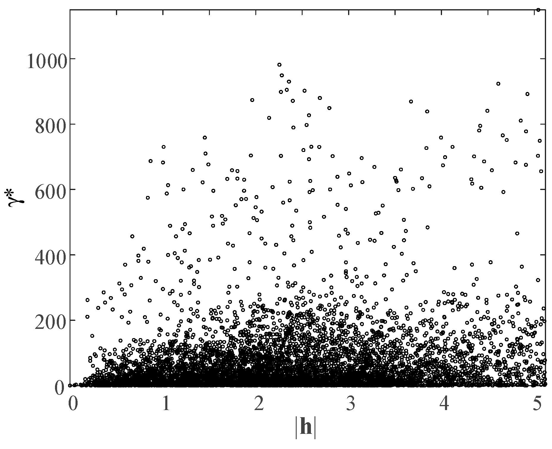
where h is a vector of the spatial separation between the two arbitrary points, while γ* for the spatial separation h can be plotted, as shown in Figure 2, which is referred to as the variogram cloud.

Figure 2 shows an example of a variogram cloud for the atmospheric refractivity data. The atmospheric refractivity data in this study is obtained from all the meteorological observatories in Korea, and detailed information about these data will be provided in Section 3. As mentioned in relation to Figure 1, γ* can be calculated using all the sample pairs in a data set. However, as can be seen in Figure 2, it is difficult to identify the clear spatial correlations between each data sample using the variogram cloud. Therefore, the separation distance Δh is applied to the variogram cloud. For example, in Figure 2, the entire spatial separation h is divided into 21 regions using the separation distance Δh = 0.25. Then, the average value of the points of the variogram cloud in each region is derived, which is termed the experimental variogram.

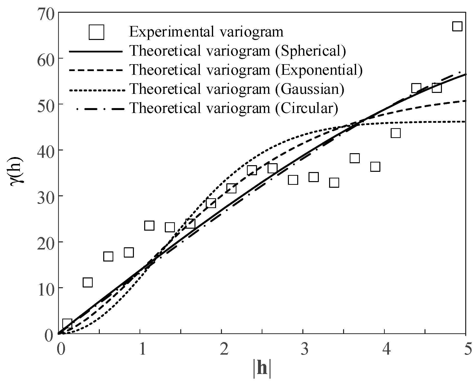
Figure 3 presents the experimental and theoretical variograms. The black square marks indicate the experimental variogram for the variogram cloud explained in Figure 2. When compared with the variogram cloud, the experimental variogram more clearly explains the spatial correlation of the data set, as shown in Figure 3. However, since the experimental variogram has discontinuous values, theoretical variograms with continuous values should be obtained. To construct a theoretical variogram, various covariance functions, such as the spherical model (solid line), exponential model (dashed line), Gaussian model (dotted line), and circular model (dash-dotted line), can be applied to the experimental variogram, as shown in Figure 3 [18]. Subsequently, the obtained theoretical variogram is used to calculate the weights of all the sample points [18].

3. Data Normalization of the Atmospheric Refractive Index

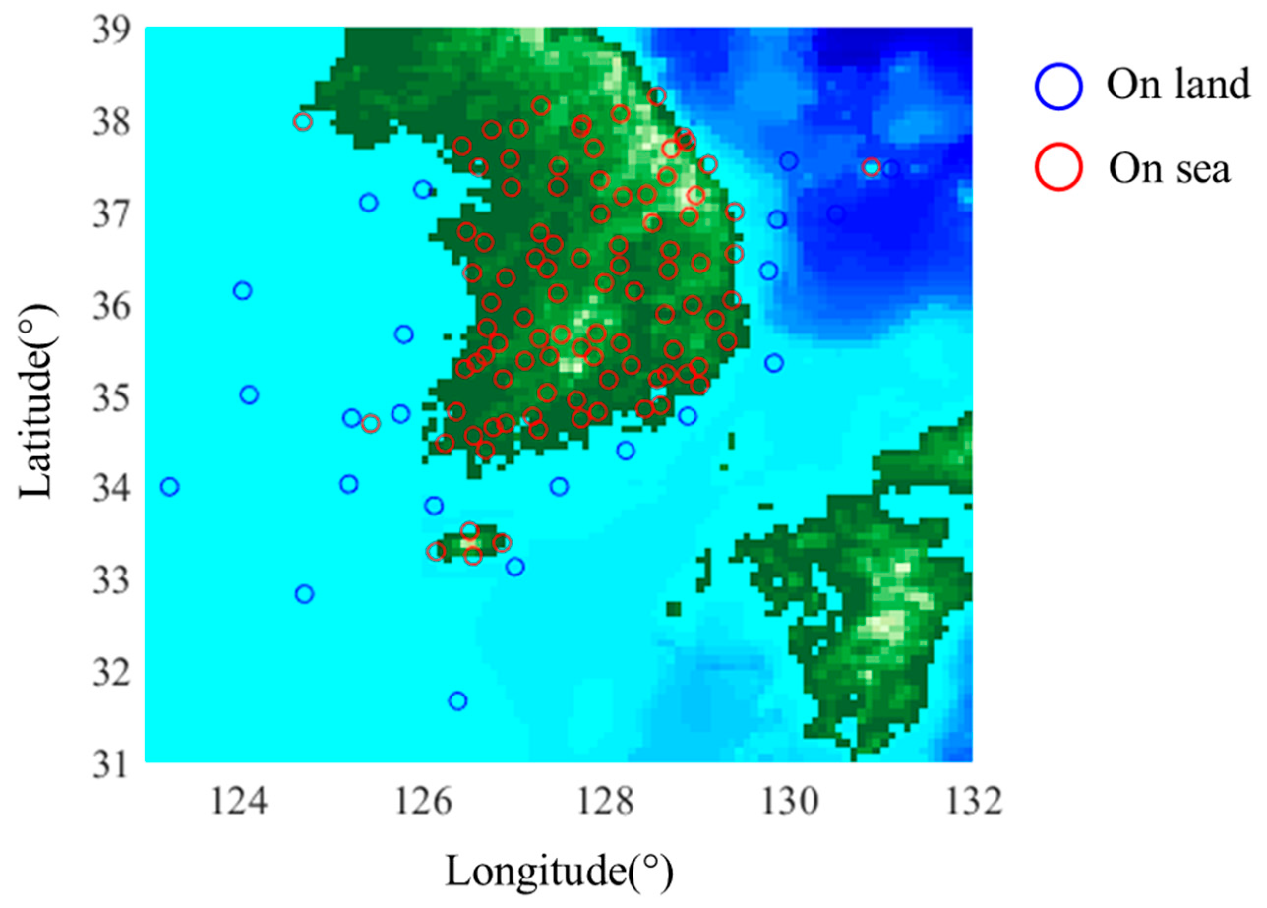
Figure 4 illustrates the locations of all the meteorological observatories in Korea. The red and blue circles indicate the locations of the meteorological observatories on the land (96 points) and on the sea (24 points), respectively. To obtain a reliable interpolation result for the atmospheric refractivity, we collect as much data as possible from all the meteorological observatories. With the collected measurement data, the atmospheric refractivity can be obtained using the following equation [16].

$$x=25.22\left(\frac{T-273.2}{T}\right)-5.31\left(\log \frac{T}{273.2}\right)$$

(4)

$$e_s=6.105h_r\cdot \frac{e^x}{100}$$

(5)

$$N=\left(77.6\times {10}^{-6}\times \frac{P}{T}+0.373\times \frac{e_s}{T^2}\right)\times {10}^6$$

(6)

where P is the air pressure in hPa, and h_r is relative humidity. e_s is the water vapor pressure in millibars, and T means the absolute temperature in K. Since the air density gradually decreases as altitude increases, the atmospheric refractive index N is also affected by the altitude at which the data are measured.

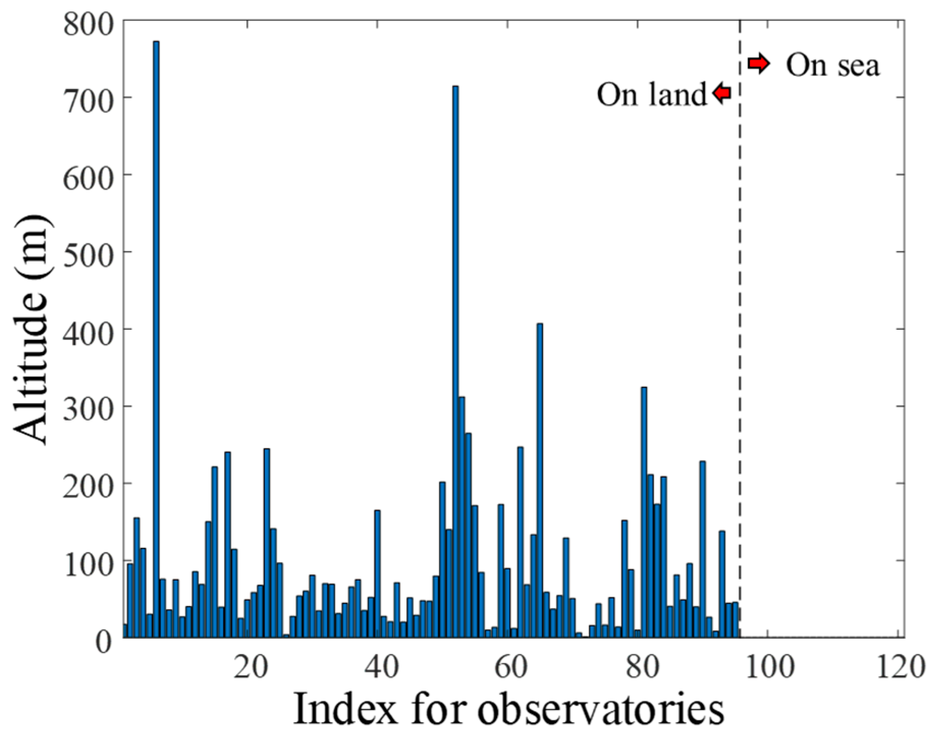
Figure 5 presents all the altitudes of the meteorological observatories in Korea. As can be seen in Figure 5, most of the meteorological observatories are located below 150 m in altitude, but some base stations are installed at high altitudes of over 700 m. Therefore, the altitudes of the ground stations vary from the lowest altitude of 1.4 m to the highest altitude of 772.4 m, and the altitudes of the 24 stations located on the sea are all assumed to be 0 m. Since meteorological data generally tend to vary depending on the altitude of the observation site, the atmospheric refractivity N is also affected by the altitude. Therefore, in order to eliminate deviations in the refractive index according to the altitude, the atmospheric refractivity N should be normalized to an altitude of 0 m.

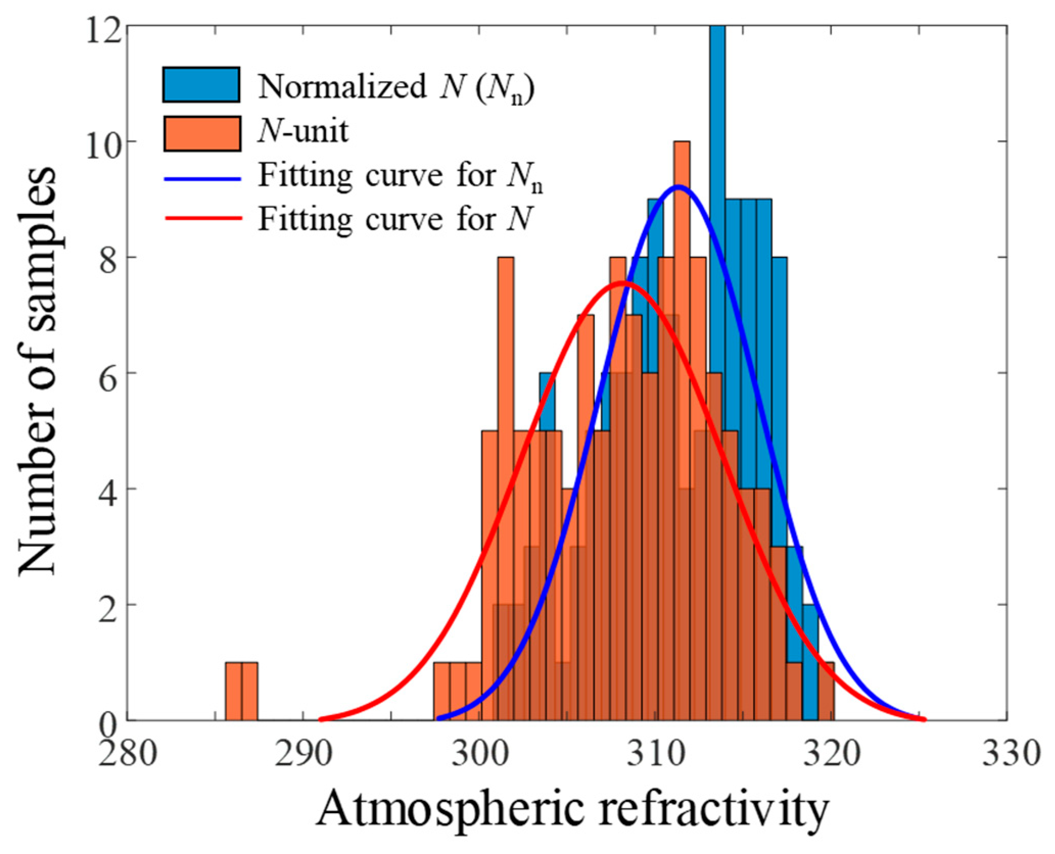
Figure 6 illustrates the histogram of the atmospheric refractivity N and normalized atmospheric refractivity N_n. These meteorological data are measured at 01:00 a.m. on 1 January 2022. Generally, under standard atmospheric conditions, the atmospheric refractive index N can be assumed to decrease by 0.039 for every 1 m increase in altitude, meaning that the normalized atmospheric refractive index N_n can be expressed by the following equation [16]:

$$N_n=N+0.039h$$

(7)

where h is the altitude of the meteorological observatory. N has an average and a variance of 308.1 and 32.7, respectively. On the other hand, N_n has an average and a variance of 311.3 and 20.6, respectively. The result demonstrates that the normalized atmospheric refractive index N_n has a smaller variance and a higher average when compared with N, because the deviation in the refractive index according to the altitude has been removed.

4. Kriging Interpolation

Figure 7 shows the average and maximum estimation errors of the Kriging interpolation according to the variogram models. To calculate the estimation error, we perform the following procedure: First, the value of one arbitrary region is removed from the collected data of all 120 regions. Then, the interpolation is performed using the data of 119 regions without the value of the arbitrarily removed region. Finally, for the removed region, we calculate the difference between the actual and interpolated values. This procedure is performed iteratively for all 120 regions, and then the average of the errors obtained for each region is calculated. In Figure 7, we also compare the average errors according to the variogram models such as spherical, exponential, Gaussian, and circular models. When using the spherical model with the Kriging method, the average and maximum errors are 0.24 and 1.32, respectively, which are the smallest values when compared with the errors obtained when using the other models.

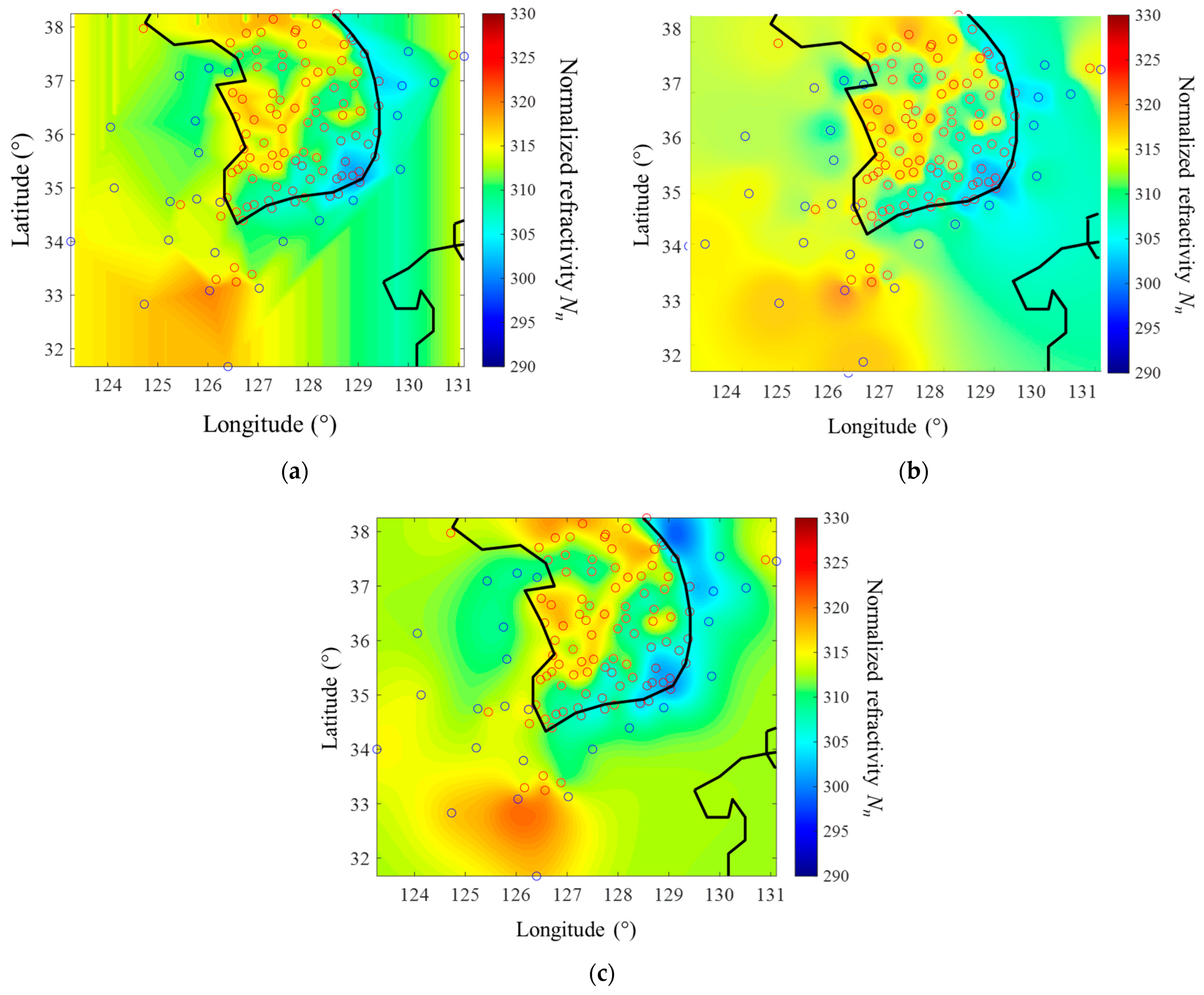
Figure 8 presents the interpolation and extrapolation results for Korea obtained using the normalized atmospheric refractivity N_n. These results are obtained using the Kriging, bi-linear, and IDW methods, respectively. The average and maximum errors of the interpolation results are listed in

Table 1. Estimation errors according to interpolation methods.

Estimation Method	Average Error	Maximum Error
Kriging	0.24	1.32
Bi-linear	1.97	8.4
IDW	3.81	11.34

. From the results, when using the Kriging method, the average and maximum errors are 0.24 and 1.32, respectively. The result demonstrates that the Kriging method can obtain better estimation results than the other interpolation methods.

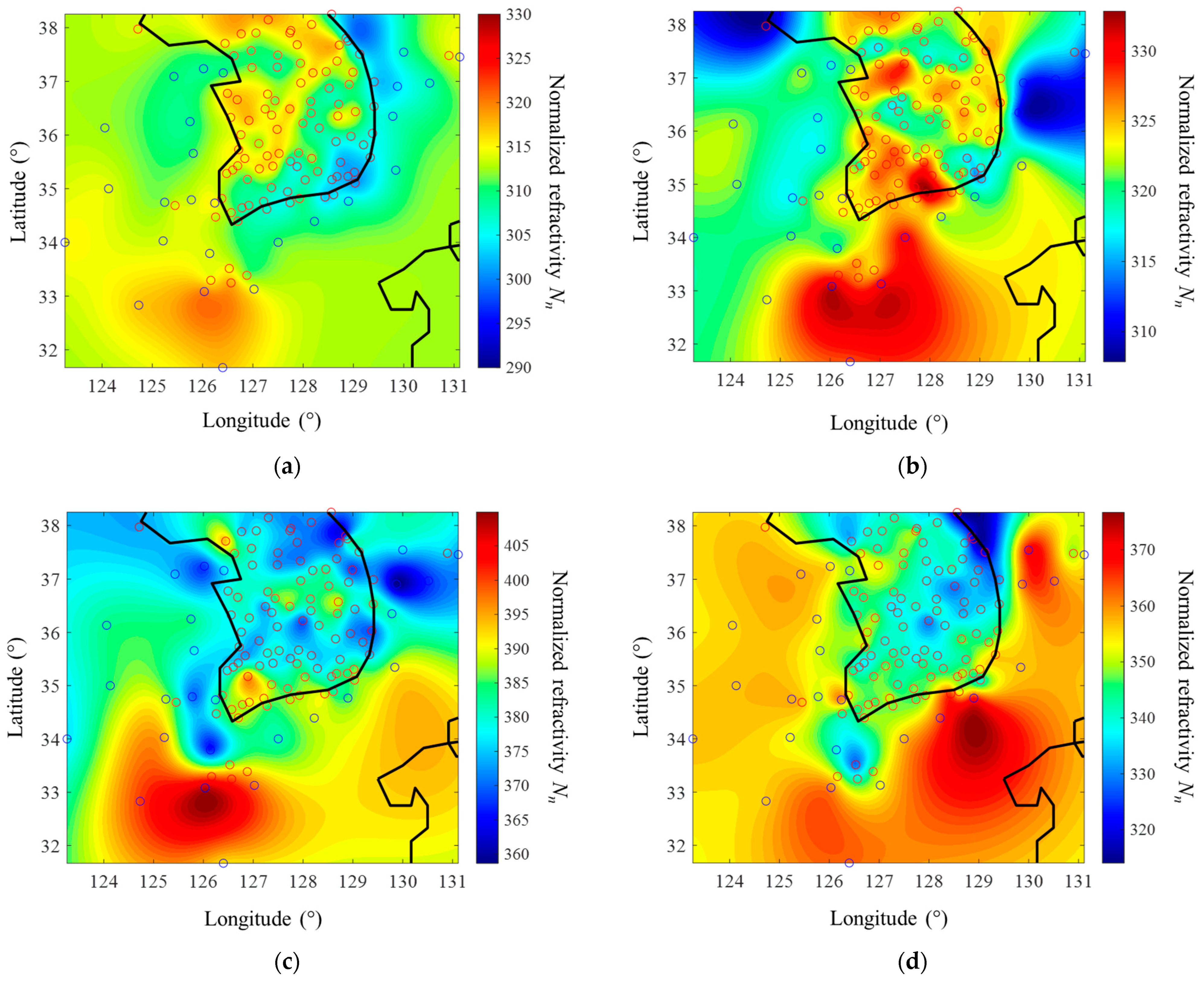
Figure 9 shows the results of the Kriging interpolation using four-season data covering winter (1 January 2022), spring (1 April 2022), summer (1 July 2022), and fall (1 October 2022). The average and maximum errors of the interpolation results are summarized in

Table 2. Summary of the estimation results for the four-season data.

Season	Average Error on Land	Maximum Error on Land	Average Error on Sea	Maximum Error on Sea
Winter	0.28	1.32	0.12	0.58
Spring	0.26	1.12	0.16	0.69
Summer	0.51	7.83	0.32	0.93
Fall	0.53	4.12	0.5	2.44

. The average estimation errors of the interpolated winter data are observed to be low (on land: 0.28; on sea: 0.12). On the other hand, in the summer, the average errors are increased (on land: 0.51; on sea: 0.32). The maximum errors are also higher in summer (on land: 7.83; on sea: 0.93) than in winter (on land: 1.32; on sea: 0.58). In all the cases in Table 2, the estimation errors on the land are higher than those on the sea.

Table 3. Summary of the estimation results for the four-season data (1 month).

Season	Average Error	Maximum Error
Winter	0.25	3.25
Spring	0.38	8.78
Summer	0.69	12.21
Fall	0.62	14.01

shows the results of examining the average and maximum errors using the four-season data after expanding the data observation period to 1 month. The Kriging interpolation method can estimate the atmospheric refractivity with low average and maximum errors of less than 0.38 and 8.78, respectively. In addition, similar to the results in Table 2, the average error and maximum error for one month’s data are found to be smaller in winter than in summer.

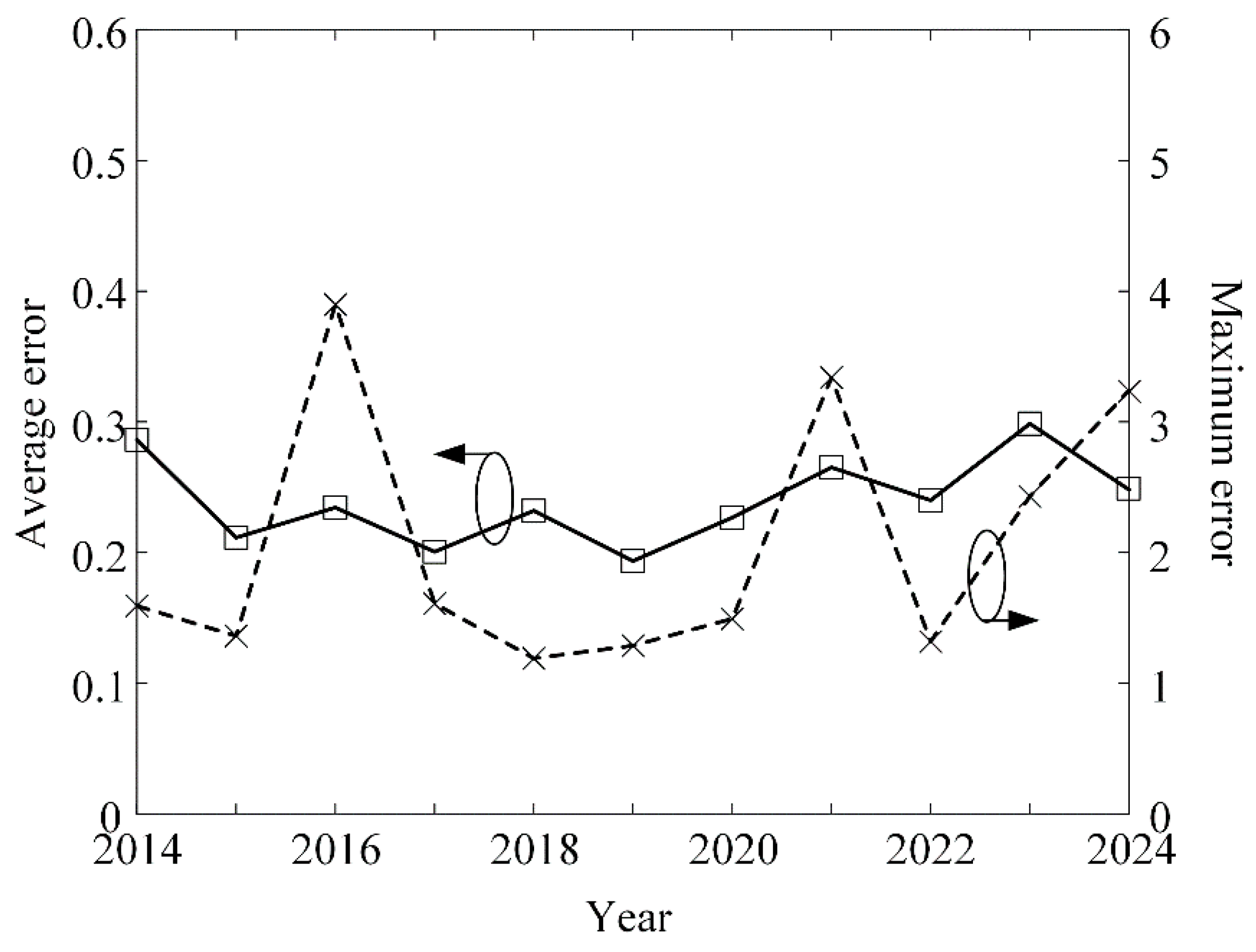
Figure 10 shows the average and maximum estimation errors of the Kriging interpolation on January 1 of each year from 2014 to 2024. The average estimation errors remained in the range of 0.19 to 0.3 over the 11 years, and the maximum estimation errors remained in the range of 1.29 to 3.89 during the same period. This result means that for the same date, the estimation error does not change significantly if the year changes.

5. Conclusions

We investigated the Kriging interpolation method for the construction of the database of atmospheric refractivity in Korea. To collect as much data as possible for the interpolation, meteorological data from 120 regions of Korea, including both land and sea areas, were examined. The normalized atmospheric refractivity N_n was then calculated for an altitude of 0 m. To obtain accurate Kriging interpolation results, we examined the estimation error of the Kriging interpolation results when using various variogram models such as spherical, exponential, Gaussian, and circular models. The result of the Kriging interpolation with the spherical variogram model had the lowest average and maximum estimation errors of 0.24 and 1.32, respectively. This result demonstrated that the Kriging method can obtain better estimation results than the conventional interpolation methods. In addition, the estimation accuracy of the Kriging interpolation method for the four seasons was investigated. The average and maximum estimation errors of the interpolated winter data were low at 0.25 and 3.25, respectively. On the other hand, in the summer, the average and maximum errors were as high as 0.69 and 12.21, respectively.

References

1. Locker, C.; Vaupel, T.; Eibert, T.F. Radiation efficient unidirectional low-profile slot antenna elements for X-band application. IEEE Trans. Antennas Propag. 2005, 53, 2765–2768. [Google Scholar] [CrossRef]
2. Dastkhosh, A.R.; Oskouei, H.D.; Khademevatan, G. Compact low weight high gain broadband antenna by polarization-rotation technique for X-band radar. Int. J. Antennas Propag. 2014, 2014, 1–10. [Google Scholar] [CrossRef]
3. Zhou, Y.; Wang, T.; Hu, R.; Su, H.; Liu, Y.; Liu, X.; Suo, J.; Snoussi, H. Multiple kernelized correlation filters (MKCF) for extended object tracking using X-band marine radar data. IEEE Trans. Signal Process. 2019, 67, 3676–3688. [Google Scholar] [CrossRef]
4. Wang, A.; Krishnamurthy, V. Signal interpretation of multifunction radars: Modeling and statistical signal processing with Stochastic Context Free Grammar. IEEE Trans. Signal Process. 2008, 56, 1106–1119. [Google Scholar] [CrossRef]
5. Wang, S.; Jang, D.; Kim, Y.; Choo, H. Design of S/X-Band dual-loop shared-aperture 2 × 2 array antenna. J. Electromagn. Eng. Sci. 2022, 22, 319–325. [Google Scholar] [CrossRef]
6. Lim, T.H.; Go, M.; Seo, C.; Choo, H. Analysis of the target detection performance of Air-to-Air airborne radar using long-range propagation simulation in abnormal atmospheric conditions. Appl. Sci. 2020, 10, 6440. [Google Scholar] [CrossRef]
7. Lim, T.; Choo, H. Prediction of target detection probability based on air-to-air long-range scenarios in anomalous atmospheric environments. Remote Sens. 2021, 13, 3943. [Google Scholar] [CrossRef]
8. Sharma, V.; Kumar, L. Photonic-radar based multiple-target tracking under complex traffic-environments. IEEE Access 2020, 8, 225845–225856. [Google Scholar] [CrossRef]
9. Kim, I.; Kim, H.; Lee, J.-H. Theoretical minimum detection range for a rapidly moving target and an experimental evaluation. J. Electromagn. Eng. Sci. 2021, 21, 161–164. [Google Scholar] [CrossRef]
10. Tedesco, M.; Wang, J.R. Atmospheric correction of AMSR-E brightness temperatures for dry snow cover mapping. IEEE Geosci. Remote Sens. Lett. 2006, 3, 320–324. [Google Scholar] [CrossRef]
11. Wang, J.R.; Racette, P.; Triesky, M.E.; Browell, E.V.; Ismail, S.; Chang, L.A. Profiling of atmospheric water vapor with MIR and LASE. IEEE Geosci. Remote Sens. Lett. 2002, 40, 1211–1219. [Google Scholar] [CrossRef]
12. Birkemeier, W.P.; Duvosin, P.F.; Fontaine, A.B.; Thomson, D.W. Indirect atmospheric measurements utilizing rake tropospheric scatter techniques—Part II: Radiometeorological interpretation of rake channel-sounding observations. Proc. IEEE 1969, 57, 552–559. [Google Scholar] [CrossRef]
13. Wang, S.; Lim, T.H.; Oh, K.; Seo, C.; Choo, H. Prediction of wide range two-dimensional refractivity using an IDW interpolation method from high-altitude refractivity data of multiple meteorological observatories. Appl. Sci. 2021, 11, 1431. [Google Scholar] [CrossRef]
14. S.-Rama, B.; Lopez, R.N.; Rio, V.S.; Darlington, T. Radar-based refractivity maps using geostatistical interpolation. IEEE Geosci. Remote Sens. Lett. 2023, 20, 3509205. [Google Scholar]
15. Yang, J.; Heo, J.; Kim, J.; Park, Y.; Choo, H.; Park, Y.B. Predicting atmospheric refractivity over the Korean peninsula using deep learning techniques. J. Korean Inst. Electromagn. Eng. Sci. 2023, 34, 493–496. [Google Scholar] [CrossRef]
16. ITU. The Radio Refractive Index: Its Formula and Refractivity Data. ITU-R P.453. 2019. Available online: https://www.itu.int/rec/R-REC-P.453/en (accessed on 8 September 2019).
17. Korea Meteorological Administration, National Climate Data Center. Available online: https://data.kma.go.kr/resources/html/en/aowdp.html (accessed on 31 October 2023).
18. Wackernagel, H. Multivariate Geostatistics, 3rd ed.; Springer: Berlin/Heidelberg, Germany, 2003. [Google Scholar]
Figure 1. Kriging interpolation.
Remotesensing 16 02379 g001
Figure 2. Example of a variogram cloud that includes all the dissimilarities (γ*) for the data set.
Remotesensing 16 02379 g002
Figure 3. Experimental and theoretical variograms.
Remotesensing 16 02379 g003
Figure 4. Locations of the observatories in Korea.
Remotesensing 16 02379 g004
Figure 5. Altitude of the meteorological observatories in Korea.
Remotesensing 16 02379 g005
Figure 6. Histograms of the N and Nn for the atmospheric measurement data.
Remotesensing 16 02379 g006
Figure 7. Average and maximum estimation errors of the Kriging interpolation according to the variogram models.
Remotesensing 16 02379 g007
Figure 8. Comparison of the interpolation results for 1 January 2022: (a) Bi-linear; (b) IDW; (c) Kriging.
Remotesensing 16 02379 g008
Figure 9. Kriging interpolation results for the four-season data: (a) winter; (b) spring; (c) summer; (d) fall.
Remotesensing 16 02379 g009
Figure 10. Kriging interpolation results for data on January 1 of each year from 2014 to 2024.
Remotesensing 16 02379 g010