Article

Inversion of Farmland Soil Moisture Based on Multi-Band Synthetic Aperture Radar Data and Optical Data

1
Beijing Institute of Space Mechanics & Electricity, Beijing 100094, China
2
College of Computer and Information Engineering, Henan University, Kaifeng 475004, China
*
Author to whom correspondence should be addressed.
Remote Sens. 2024, 16(13), 2296; https://doi.org/10.3390/rs16132296
Submission received: 11 May 2024 / Revised: 19 June 2024 / Accepted: 20 June 2024 / Published: 24 June 2024
(This article belongs to the Special Issue SAR-Based Signal Processing and Target Recognition (Second Edition))

Abstract

:
Surface soil moisture (SSM) plays an important role in agricultural and environmental systems. With the continuous improvement in the availability of remote sensing data, satellite technology has experienced widespread development in the monitoring of large-scale SSM. Synthetic Aperture Radar (SAR) and optical remote sensing data have been extensively utilized due to their complementary advantages in this field. However, the limited information from single-band SARs or single optical remote sensing data has restricted the accuracy of SSM retrieval, posing challenges for precise SSM monitoring. In contrast, multi-source and multi-band remote sensing data contain richer and more comprehensive surface information. Therefore, a method of combining multi-band SAR data and employing machine learning models for SSM inversion was proposed. C-band Sentinel-1 SAR data, X-band TerraSAR data, and Sentinel-2 optical data were used in this study. Six commonly used feature parameters were extracted from these data. Three machine learning methods suitable for small-sample training, including Genetic Algorithms Back Propagation (GA-BP), support vector regression (SVR), and Random Forest (RF), were employed to construct the SSM inversion models. The differences in SSM retrieval accuracy were compared when two different bands of SAR data were combined with optical data separately and when three types of data were used together. The results show that the best inversion performance was achieved when all three types of remote sensing data were used simultaneously. Additionally, compared to the C-band SAR data, the X-band SAR data exhibited superior performance. Ultimately, the RF model achieved the best accuracy, with a determinable coefficient of 0.9186, a root mean square error of 0.0153 cm3/cm3, and a mean absolute error of 0.0122 cm3/cm3. The results indicate that utilizing multi-band remote sensing data for SSM inversion offers significant advantages, providing a new perspective for the precise monitoring of SSM.

Graphical Abstract

1. Introduction

Surface soil moisture (SSM) plays an important role in hydrological, agricultural, and environmental systems [1]. It is one of the most important sources of material on which land plants and soil organisms depend [2]. In addition, it is a major parameter for agricultural yield estimation, crop growth monitoring, and farm irrigation [3,4,5]. Therefore, it is extremely important to obtain accurate and reliable information on SSM.
The traditional SSM measurements are generally made using SSM meters or ground-based observatories [6]. More accurate results can be obtained using SSM instruments, but this method is time-consuming and labor-intensive [7,8]. In contrast, ground observation stations do not rely on manpower. However, the limited number of sampling points makes it difficult to accurately and effectively monitor large areas of SSM information [9,10]. SSM is characterized by high temporal heterogeneity and high spatial variability [2]. This makes it even more difficult for traditional SSM measurement methods to meet the needs of practical applications [11]. Remote sensing technology, with the advantages of wide coverage and high temporal resolution, has gradually become the main means of monitoring SSM on a large scale [12,13,14].
In the study on SSM inversion using remote sensing data, the data mainly originate from microwave remote sensing and optical remote sensing technologies [15]. Optical remote sensing has the advantages of high spatial resolution, large width, and easy data acquisition [16]. However, it has a weak ability to penetrate the ground surface and is susceptible to weather conditions, such as clouds, rain, and fog [17]. Synthetic Aperture Radar (SAR), as a kind of microwave remote sensing, has the characteristic of all-time, all-weather, and strong penetration capability [18]. However, it is susceptible to surface morphology and vegetation cover, and the modeling is relatively complex. In the study of SSM inversion, SSM information is mainly reflected by radar backscattering coefficients. In farmland areas, the presence of a vegetation layer affects the radar backscatter coefficient. Therefore, eliminating the influence of vegetation to obtain the corrected soil backscatter coefficient is a crucial step in SSM inversion. The vegetation indices extracted from the optical remote sensing data can reflect certain unique properties or features of the vegetation. Therefore, many studies have been carried out on the collaborative inversion of SSM using multi-source data from both optical and SAR remote sensing [19]. Ma et al. proposed an algorithm that utilized Sentinel-1 and Sentinel-2 data to simultaneously retrieve SSM, surface roughness, and vegetation water content [20]. Liu et al. employed various machine learning algorithms and semi-empirical models in combination with Sentinel-1A and Sentinel-2A data to estimate SSM in farmland and found that the Random Forest (RF) algorithm achieved the highest accuracy in estimating SSM when combining SAR and optical images [21].
However, with the increasing availability of SAR data, solely relying on the combination of Sentinel-1 and Sentinel-2 remote sensing data for SSM retrieval is still insufficient for more accurate SSM inversion. Multi-band SAR data can provide more comprehensive and richer surface information [22,23,24,25]. Therefore, exploring the effectiveness of using multi-band remote sensing data for SSM retrieval is of great significance. The powerful fitting capabilities of machine learning techniques enable the collaborative use of multi-band remote sensing data for SSM retrieval [26,27,28]. It can solve the complex nonlinear problem between surface parameters, vegetation index, and radar backscattering coefficients [29,30]. Therefore, many scholars have started to combine multi-band (C-, L-, X-, etc.) SAR remote sensing data and machine learning methods for the inversion of SSM [31,32,33]. Balenzano et al. combined change detection techniques, using C-band and L-band SAR data, for time-series agricultural SSM inversion and found that for crops relatively insensitive to volume scattering in the vegetation canopy, the proposed method could be used throughout the entire growing season [34]. Kseneman et al. achieved promising results by employing Tikhonov regularization and neural networks to estimate SSM based on X-band data [35]. Although these methods have achieved good results in practical applications, many machine learning models still rely on large datasets [36,37]. In fact, many regions lack ground observation stations, making it difficult to obtain a large amount of sample data. In the case of small sample datasets, high-precision SSM monitoring remains challenging.
Currently, SSM inversion research using small sample datasets has been conducted by many scholars. Chen et al. combined RF, support vector regression (SVR), and other models for SSM inversion using 240 samples and found that the RF method achieved the best inversion results in the case of small sample datasets [38]. Zhao et al. retrieved the SSM by integrating multi-source remote sensing data with machine learning methods suitable for small sample datasets, such as Genetic Algorithm-Back Propagation (GA-BP), RF, and SVR and indicated that these methods were applicable for SSM retrieval under conditions of small sample data [6]. However, the above studies only combined SAR data and optical data. Due to the limited information obtained from small sample datasets, combining multi-band SAR remote sensing data for SSM inversion may lead to better results. Therefore, SSM inversion methods using small sample datasets are studied from the perspective of multi-band remote sensing data and machine learning in this study.
Data acquired from three different remote sensing satellites, which were C-band Sentinel-1, X-band TerraSAR, and Sentinel-2, were employed in this study, combining GA-BP, SVR, and RF models to construct an SSM inversion model. The main contributions of this study can be summarized as follows: (1) Differences in the potential C-band and X-band SAR remote sensing data in SSM inversion were explored and validated. (2) The abilities of three machine learning models, GA-BP, SVR, and RF, were compared in terms of SSM inversion. (3) The parameters of the three machine learning models were optimized through the cross-validation method, demonstrating the impact of model parameters on model performance. Therefore, by combining multi-band remote sensing data, a new approach to SSM monitoring in the context of small-sample datasets was offered by this study.

2. Materials and Methods

Remote sensing data were utilized in this study, combining three machine learning methods suitable for small sample datasets to compare the potential of multi-band remote sensing data in estimating SSM. Section 2.1 briefly describes the study area. Section 2.2 describes the datasets used and the pre-processing of the images. Section 2.3 describes in detail the techniques and methods used in this experiment.

2.1. Study Area

The study area, as shown in Figure 1, is located in the east of the Danjiangkou reservoir ecological service area, which is at the junction of Henan and Hubei provinces, China. The local climate falls under the category of a subtropical monsoon climate with mild and semi-humid conditions [39]. The annual average temperature is 15–17 °C, and the annual average precipitation fluctuates between 700 and 1100 mm [40,41]. This climatic condition provides a favorable environment for the growth of winter wheat and other crops. During the study period, winter wheat was the primary vegetation type in the study area.

2.2. Dataset and Image Preprocessing

The datasets utilized in this study primarily include satellite remote sensing data and ground observation data. The satellite remote sensing data encompass three types: Sentinel-1, TerraSAR, and Sentinel-2.
This study employed Sentinel-1 data in the Interferometric Wide (IW) mode with the Ground Range Detection (GRD) format. These data were obtained from the website https://browser.dataspace.copernicus.eu, accessed on 20 September 2022. Two SAR images from 23 September 2021 and 16 December 2021 were selected. Subsequently, preprocessing operations were conducted on these two images. Sentinel-1 data were preprocessed using the Sentinel Application Platform (SNAP) version 8.0, including steps such as orbit correction and radiometric calibration.
This study employed single-polarization TerraSAR data in the scanning mode with the Multi-Look Ground-Range-Detected (MGD) format. These data were obtained from the website https://sss.terrasar-x.dlr.de, accessed on 20 September 2022. Two SAR images from 24 September 2021 and 21 December 2021 were selected. Subsequently, preprocessing operations were conducted on these two images. TerraSAR data were preprocessed using Sarscape software version 5.6, including multi-looking, filtering, radiometric calibration, geocoding, and registration.
The Sentinel-2 data at the L2A processing level were employed in this study. These data were obtained from the website https://browser.dataspace.copernicus.eu, accessed on 20 September 2022. Based on the acquisition dates of Sentinel-1 SAR images and considering the impact of adverse weather conditions, two optical images from 22 September 2021 and 21 December 2021 were selected.
To ensure that remote sensing images with different resolutions could be accurately compared and analyzed at the same spatial scale, Sentinel-1 images were utilized as the reference for image registration and resampling in this study. In the end, the resolution of all three remote sensing data was 10 m.
The SSM data used in this study were obtained through two field measurements. In each field measurement, dozens of sampling plots were randomly and uniformly chosen in the study area. A group of measured data was collected in each sampling plot and included the SSM values (vol.%) and the latitude and longitude coordinates of the sampling plot. SSM values were measured at five positions at each sampling plot using a portable SSM instrument TDR350, and their average value was taken as the final SSM value of this sampling plot. Simultaneously, a portable UG905 locator was used to locate the sampling plots. A total of 90 groups of sample data were collected in the study area during the two field trips. Regarding this, 41 groups among them were obtained on 23 September 2021, and the other 49 groups were obtained on 21 December 2021, with specific locations depicted in Figure 1b. More detailed information on the characteristics of the data used is presented in Table 1. During the satellite transit and ground observation, there was no clear precipitation or temperature change in the study area. The SSM values and surface roughness in the study area on 22 September, 23 September, and 24 September 2021 were almost constant.

2.3. Methodology

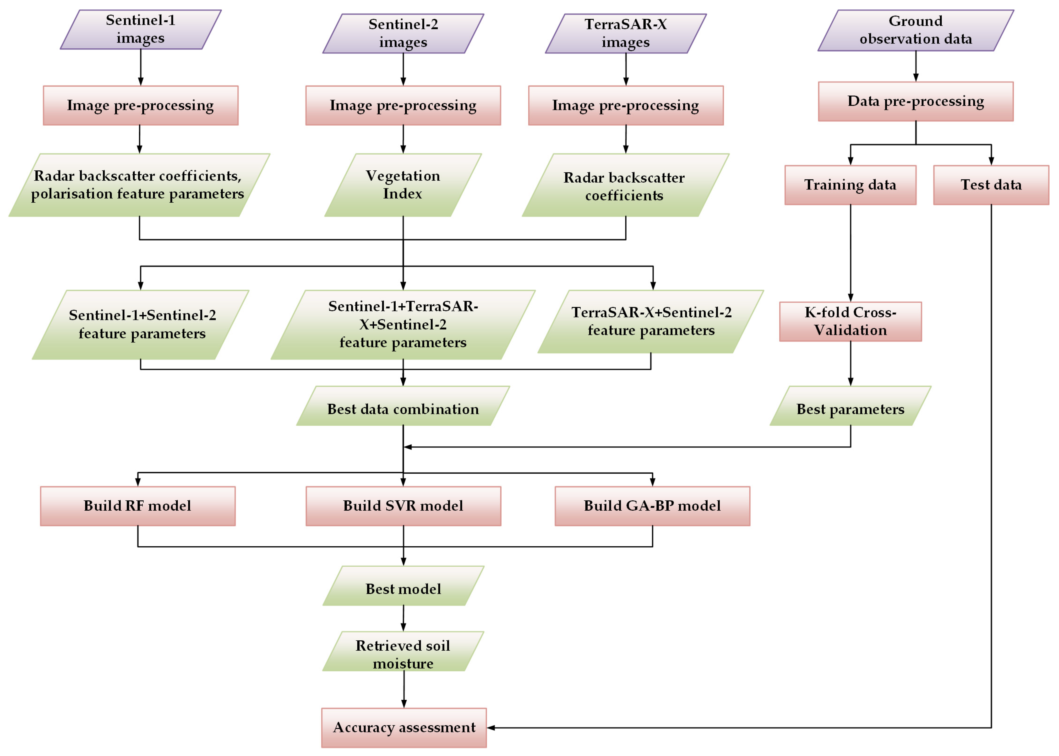
This study began by extracting feature parameters from remote sensing data, which were then combined into three different sets. Subsequently, machine learning models were employed to assess the potential of different bands of remote sensing data for SSM inversion. Based on the evaluation results, the optimal parameter combination was selected. Following this, 10-fold cross-validation was used to adjust the parameters of the machine learning model, aiming to obtain the best model. Finally, the optimal data combination and the best model were employed for SSM inversion in the study area. The technology roadmap for this approach is shown in Figure 2.

2.3.1. Feature Parameters Extraction

Using backscattering information from SAR data and vegetation index information from optical data for parameter inversion modeling is a common method in SSM inversion [42]. Feature parameters were extracted from both SAR remote sensing data and optical remote sensing data to establish the SSM inversion model in this study.
  • Feature Parameters Extracted from SAR Data
The monitoring of SSM in farmland using SAR data is primarily reflected through radar backscattering coefficients, which vary with the changes in SSM values [43,44]. Therefore, it is crucial to pay attention to the changes in radar backscattering coefficients. The radar backscattering coefficients are influenced by factors such as the incidence angle ( θ ), polarization mode, and wavelength. Therefore, the θ , VV, and VH images were extracted from Sentinel-1 data, along with the HH images from TerraSAR data in this study. Subsequently, corresponding data were extracted from these images for the ground observation plots.
  • Feature Parameters Extracted from Optical Images
In wheat fields planted in September and December, the structure of wheat plants can influence radar backscatter. This results in the radar receiving backscatter signals that include both soil backscatter and vegetation backscatter. Therefore, minimizing the impact of vegetation backscatter is crucial for achieving accurate SSM retrieval. In optical remote sensing data, vegetation indices can be calculated from the optical bands, providing information about surface vegetation. Therefore, vegetation indices were employed as feature parameters for SSM inversion in this study.
In the study of SSM inversion, the commonly used vegetation indices mainly include the Normalized Difference Vegetation Index (NDVI), Normalized Difference Water Index (NDWI), Ratio Vegetation Index (RVI), and Moisture Stress Index (MSI). In the fields of wheat during September and December, the growth cycle was relatively short, and the vertical vegetation height was comparatively low. Therefore, the NDVI and NDWI indices were chosen in this study to more accurately describe the actual growth conditions of wheat.
The range of NDVI values was between −1 and 1. The closer the value was to 0, the closer the study area was to bare soil, and the closer the value was to 1, the higher the vegetation vitality. The calculation formula is shown in Equation (1) [45]. The range of NDWI values was between −1 and 1. The closer the value was to 1, the higher the water content of vegetation was. Its calculation formula is shown in Equation (2) [46].
N D V I = ρ 842 ρ 665 ρ 842 + ρ 665
N D W I = ρ 842 ρ 1610 ρ 842 + ρ 1610
where ρ 665 , ρ 842 , and ρ 1610 represent the values of the bands corresponding to the 665, 842, and 1610 nm bands in the Sentinel-2 data, respectively.
In summary, a total of six feature parameters were extracted from the SAR data and optical data, as shown in Table 2.

2.3.2. Machine Learning Model Building

Feature parameters were extracted from SAR and optical data, and machine learning methods were utilized to establish relationships between input variables (such as VV, HH, NDVI, etc.) and the SSM value of ground observation. The model incorporates estimation error to achieve SSM retrieval. The relationship between SSM and different inputs can be expressed using Equations (3) and (4) [47]:
SSM = f ML ( C ) + ε
C = ( VV ,   HH ,   NDVI ,   NDWI ,   )
where S S M is the value of ground observation, ε is the model estimation error, and C is the input variable.
  • GA-BP model
GA-BP model is a model that combines a genetic algorithm (GA) and a backpropagation neural network (BPNN). BPNN is a feed-forward neural network that minimizes the error between the predicted output and the actual output. BPNN has good learning ability and powerful nonlinear simulation ability. However, due to its backpropagation feature, it is easy to fall into local minima instead of global minima, which leads to poor model performance. GA aims to find the best solution to a problem by simulating the genetic variation and selection process of genes. By combining the GA algorithm with BPNN, it is easier to obtain better models using the global search capability of the genetic algorithm to overcome the local minima problem that may be encountered in the training of BPNN [48].
  • SVR model
The SVR model can be used to solve regression problems in the case of small samples, which requires finding a regression hyperplane with the shortest distance from all samples. It has better robustness and generalization ability and can be used for different types of regression problems. However, its greatest strength is its nonlinear modeling ability, which allows it to map data to a high-dimensional feature space using kernel tricks. The SVR model can be fitted by using a linear function in high-dimensional space. The optimal kernel function k ( x i , x ) is chosen to achieve linear regression in high-dimensional space. Its prediction function is shown in Equation (5) [49]:
f ( x ) = i = 1 n ( α i α i * ) k ( x i , x ) + b
where n is the number of samples, α i , α i *   is the Lagrange operator, and b is the bias term coefficient.
  • RF model
The RF model is an integrated learning method based on multiple regression trees for solving regression problems. It is an algorithm that enhances overall performance by constructing multiple decision trees and aggregating their results. In small sample datasets, individual decision trees are prone to overfitting. However, by assembling multiple decision trees, RF can mitigate the risk of overfitting, thereby improving its generalization capability. RF not only makes numerical predictions but also determines the importance of features by calculating the contribution of the feature variables through an internal function. In addition, compared with some other regression algorithms, RF does not require many hyperparameters, so it does not need complex parameter tuning [6].
The three machine learning methods contain many different parameters that affect the performance of the final model. The adjustment of parameters in a machine learning model can reduce the impact of undesirable parameters on the effectiveness of the model. However, it will also take a lot of time if all the parameters are tuned for selection. Therefore, several key parameters in the three machine learning models were adapted in this study.
For the GA-BP model, the number of hidden layers, the number of nodes, the population size, and the number of iterations were selected to be adjusted in this study. This is because these parameters directly affect the model’s structure and training process, and adjusting them can effectively optimize the performance of the neural network. For the SVR model, the penalty parameter and the kernel coefficient were chosen to be adjusted in this study. These two parameters control the model’s complexity and the range of influence of the kernel function while adjusting them can improve the model’s prediction accuracy. For the RF model, the number of trees and the maximum depth of trees were adjusted in this study. This is because the number and depth of decision trees affect the model’s complexity and fitting ability, and adjusting these parameters can find a balance between overfitting and underfitting.

2.3.3. Data Combination Selection

Different bands of remote sensing data offer diverse information, and the sensitivities they exhibit to SSM vary. Therefore, it is crucial to delve into the potential of multi-band remote sensing data in SSM inversion. This study assessed the potential of SSM inversion using different SAR data by comparing the accuracy of C-band Sentinel-1 data and X-band TerraSAR data, each combined with Sentinel-2 optical data.
In this study, feature parameter combinations obtained from different SAR data with optical data were inputted into pre-constructed GA-BP, SVR, and RF models. Its purpose was to evaluate the SSM inversion capabilities of different SAR data by comparing the accuracies obtained from different data combinations. This also provided a basis for selecting suitable feature parameters for subsequent experiments. The way the data were combined is shown in Table 3.

2.3.4. K-Fold Cross-Validation

Cross-validation is widely recognized as an effective method for model selection and evaluation, especially for small datasets. It has the following two main roles: model selection and model evaluation. In this study, cross-validation was used to select appropriate parameters and optimize machine learning models to improve the inversion results.
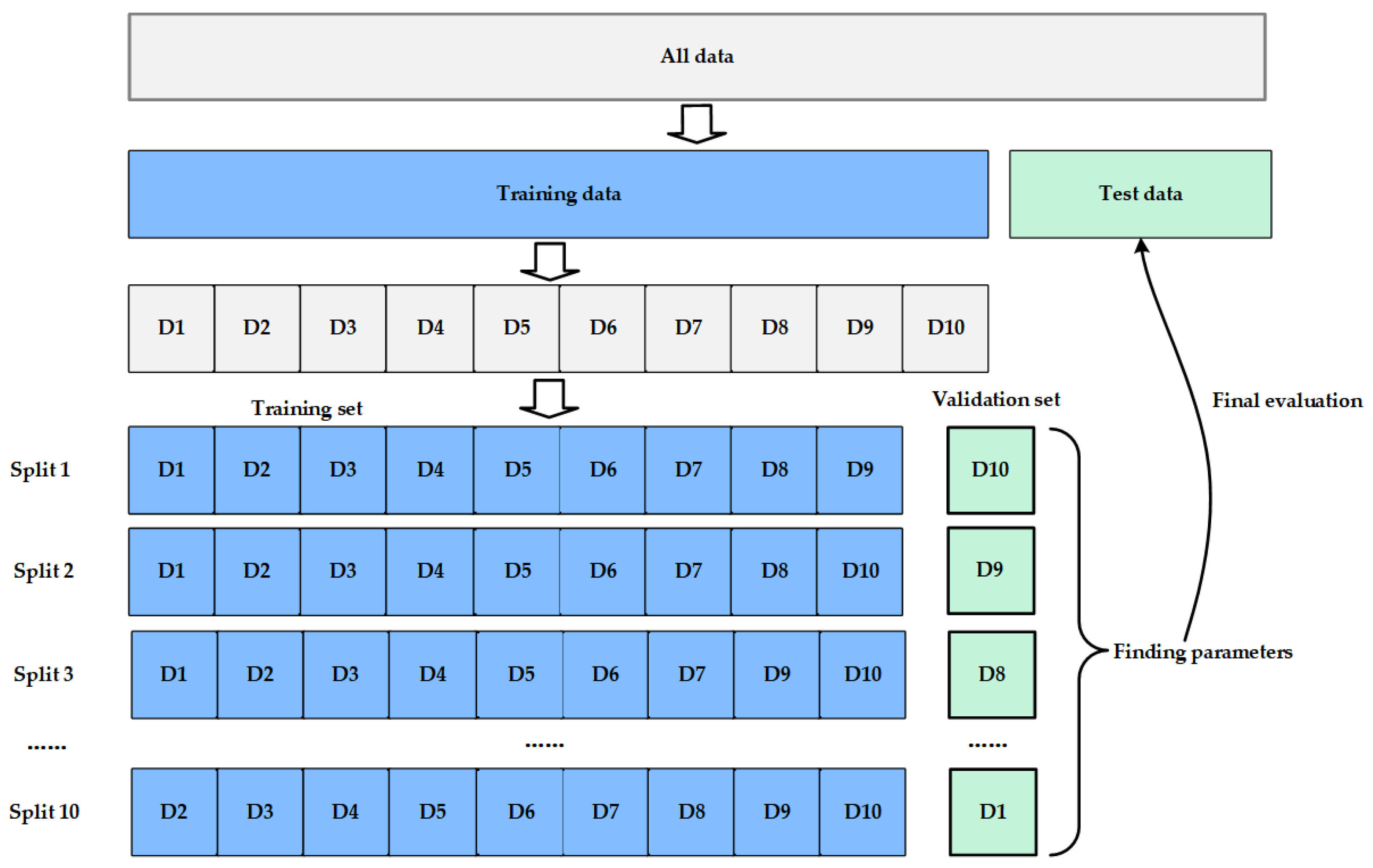
The main idea of K-fold cross-validation is to partition the dataset into two parts: the training set and the test set. The first part of the training set serves as training data for the model, while the second part acts as a validation set to assess the model’s performance. During this process, the model parameters are continuously adjusted, and the model with the smallest prediction error is selected as the optimal model. Finally, the trained model is tested for its final performance using the testing set data [50].
In machine learning, parameter selection aims to identify the optimal hyperparameters to minimize loss and enhance accuracy. In the case of a small amount of data, the selection of K-fold cross-validation is a more appropriate choice. In this study, 10-fold cross-validation was chosen. The process of model selection using the 10-fold cross-validation method is shown in Figure 3.

2.3.5. SSM Result Prediction and Accuracy Assessment

The experimental results were evaluated using three accuracy evaluation metrics: the coefficient of determination (R2), root mean square error (RMSE), and mean absolute error (MAE). Among these three evaluation indexes, the higher the R2, the better, while for the other two RMSEs, a smaller MAE represented the higher precision of the results. In order to reduce the eventuality of the experimental results, the experimental results were averaged after several experiments. The formulas for their calculation are shown in Equations (6)–(8).
R 2 = 1 i = 1 n ( y i y i ) 2 i = 1 n ( y i y ¯ ) 2
R M S E = 1 n i = 1 n ( y i y i ) 2
M A E = 1 n i = 1 n | y i y i |
where y i represents the actual measured value of SSM, ŷ i represents the model predicted value, y ¯ represents the mean actual measured value of SSM, and n represents the sample size.

3. Results

This section first compared the potential of estimating SSM using different remote sensing data bands, then compared the differences in inversion performance before and after optimizing machine learning models through cross-validation methods. Finally, combining the best model obtained from the experiments, the spatial mapping of SSM across the entire study area was conducted.

3.1. Multi-Band Data Accuracy Analysis

As shown in Table 4, there existed a significant difference in the accuracy of the SSM inversion when combining C-band and X-band SAR remote sensing data with optical remote sensing data using three machine learning models. From the table, it was evident that the potential of different machine learning models combined with various remote sensing data combinations for SSM inversion was compared in this study.
Firstly, in terms of the ability of different machine learning models to invert SSM. It was found that among the three models, GA-BP, SVR, and RF, RF consistently outperformed the other two models regardless of the combination used. When combining Sentinel-1 with Sentinel-2, the optimal RF model performed significantly better than the GA-BP model, with differences of 0.1249 in R2, 0.009 cm3/cm3 in RMSE, and 0.0147 cm3/cm3 in MAE. Furthermore, when using the other two data combinations, the RF model generally exhibited the best performance. This occurrence may be attributed to the inherent structure of the RF model. The RF model is an ensemble learning method based on decision trees, enabling it to mitigate errors from individual trees through majority voting or averaging. Additionally, compared to GA-BP and SVR, the RF model exhibits greater versatility. In summary, in the case of a small sample dataset, selecting the RF model among the three machine learning models is more likely to achieve better SSM inversion results.
Secondly, in terms of the ability of SSM inversion to use different bands of remote sensing data, regardless of which machine learning model was used, the results showed higher accuracy when Sentinel-1 SAR data, TerraSAR SAR data, and Sentinel-2 optical data were used simultaneously. For instance, in the RF model, the R2 value reached 0.8812 when both SAR data were combined with optical data. However, the value was only 0.7535 when using C-band data alone and 0.8306 when using X-band data alone. The effectiveness of using multiple bands simultaneously was significantly better than using a single band. This suggests that combining multi-band SAR data with optical data for inversion improves accuracy, validating the effectiveness of multi-wavelength SAR data in SSM inversion. Additionally, in terms of the performance of SAR data inversion using single bands, the X-band SAR data generally outperforms the C-band SAR data. The reason for this may lie in the different sensitivities of SAR data from different bands to surface roughness. Surface roughness still had a significant impact on SSM inversion in wheat fields in September and December. In this study, the influence of roughness accuracy was not considered when using SAR data from both bands for SSM inversion. However, X-band SAR data were less sensitive to surface roughness, resulting in less influence from roughness compared to the C-band, thereby yielding better inversion results.
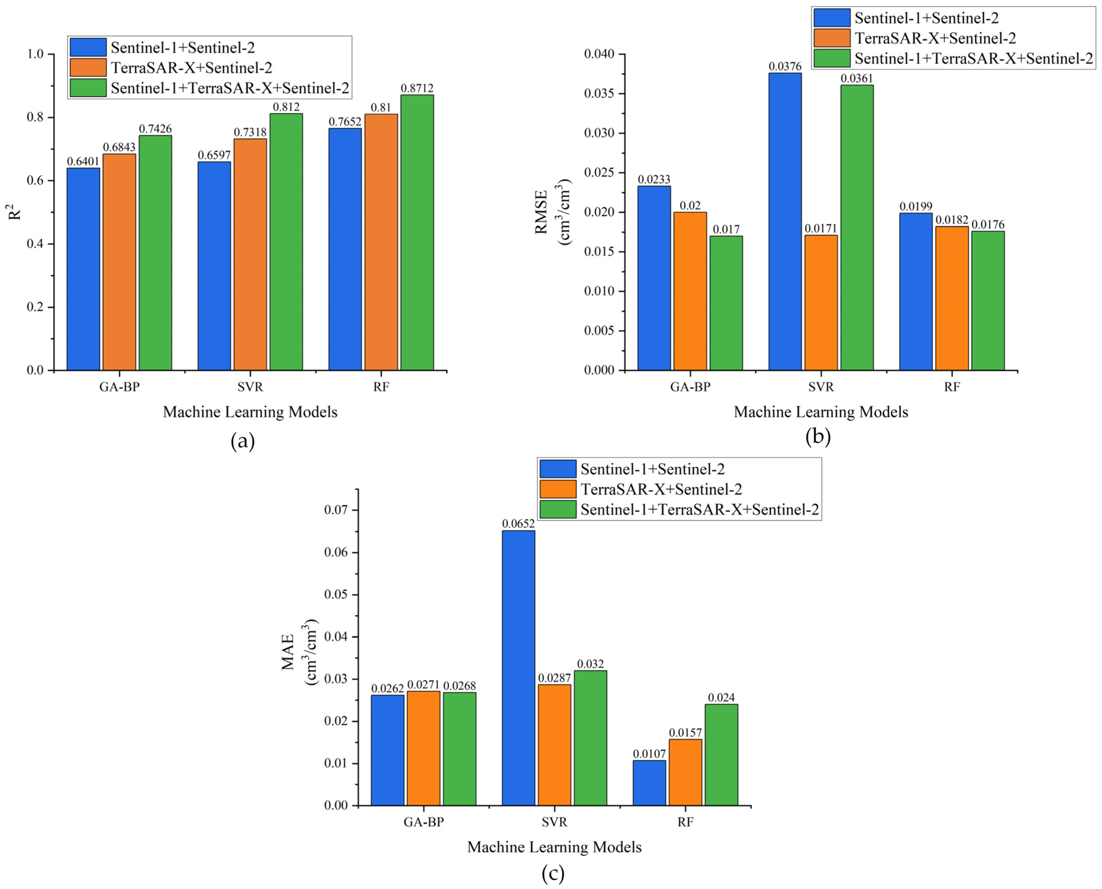
The R2, RMSE, and MAE results of the model on the training set are shown in Figure 4. Compared with the test set, it could be seen that the model did not exhibit overfitting or underfitting. Furthermore, the combination of Sentinel-1, Sentinel-2, and TerraSAR data (green bars) achieved the best overall performance. This indicates that the combined use of multi-band remote sensing data could significantly enhance the model’s performance.

3.2. Cross-Validation Accuracy Analysis

In this paper, a 10-fold cross-validation method was used to select the parameters in GA-BP, SVR, and RF by three machine learning methods. This method allows for the more adequate use of small sample data, thus improving the performance and the generalization of the model.
This study combines feature parameters extracted from different remote sensing data to continuously adjust the parameters of GA-BP, SVR, and RF models, comparing their effectiveness in SSM inversion. After comparative verification, the model achieved the best results when the following parameter values were selected, as shown in Table 5.
From the above discussion, it is evident that optimal experimental results were achieved when SAR remote sensing data from the C-band and X-band were used simultaneously with optical remote sensing data. Therefore, multi-band remote sensing data, along with optical data, combined with machine learning models with optimized parameters, were employed in this study for SSM inversion. The adjusted parameters were input into the models, and then the performance of the models was validated using the test set. A comparison of the inversion results of different models is given in Table 6.
From Table 6, it can be observed that from the three machine learning models, GA-BP, SVR, and RF, RF demonstrated the best experimental results. Its R2 was 0.9186, RMSE was 0.0153 cm3/cm3, and MAE was 0.0122 cm3/cm3.
From the comparison between Table 4 and Table 6, it can be seen that the effect of SSM inversion changed after the parameters of the machine learning model were adjusted by the cross-validation method. Before adjusting the parameters, the RF model with the best accuracy was obtained, and its R2 was 0.8812, RMSE was 0.0169 cm3/cm3, and MAE was 0.0131 cm3/cm3. After adjusting the parameters, the RF model was still the best among the three machine learning models. Furthermore, by combining three different remote sensing datasets, the R2 value for SSM inversion improved from 0.7208 to 0.7346 with the GA-BP model. Meanwhile, combining the SVR model for SSM inversion saw an increase in R2 from 0.7984 to 0.8247. Compared with before, the effect of SSM inversion improved in a general trend. This indicates that the parameters of machine learning models had a significant impact on the inversion results. Adjusting the parameters of machine learning models can optimize the structure and performance of the model, thereby improving the accuracy and stability of SSM inversion.
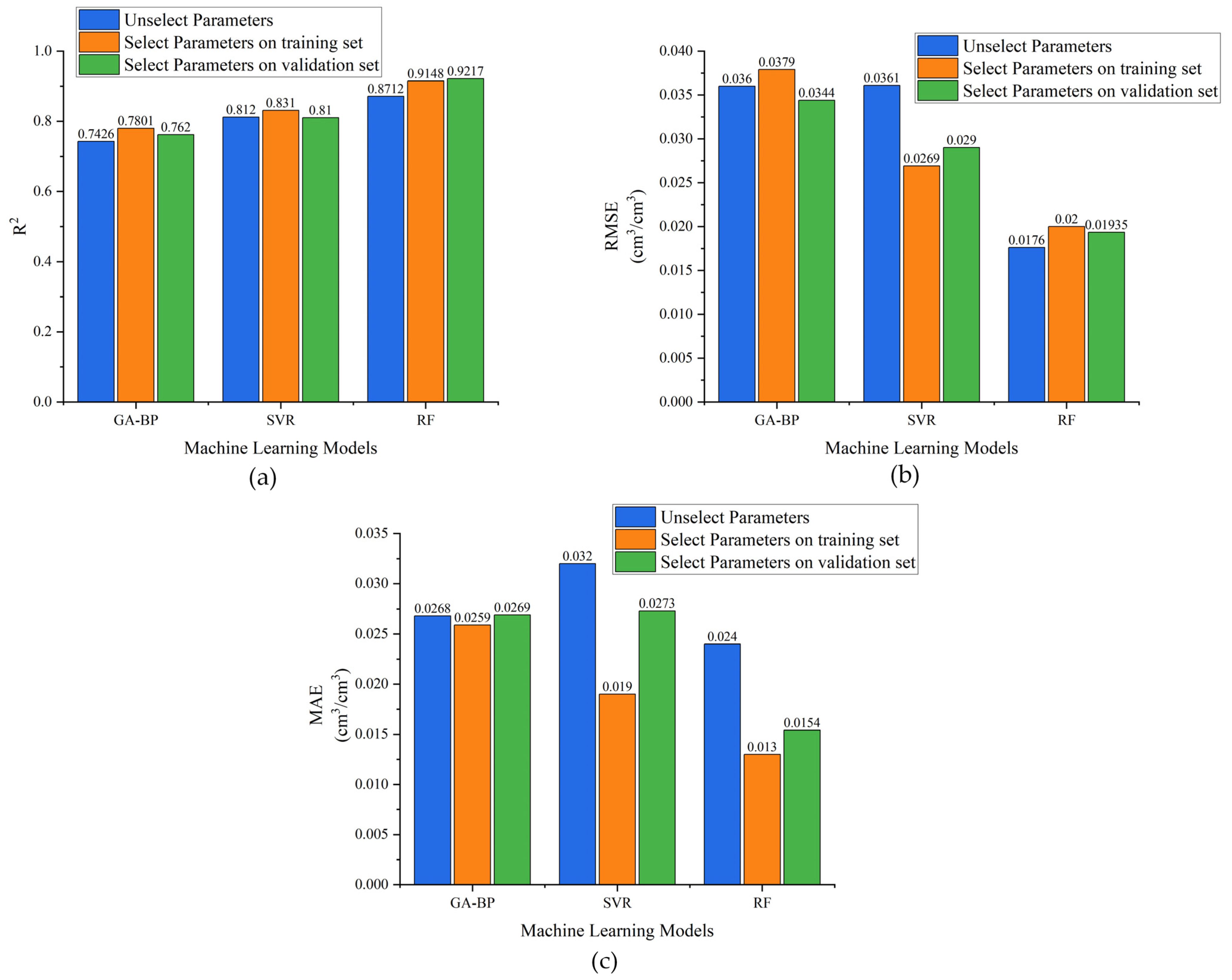
The R2, RMSE, and MAE results of the model on the training set and validation set are shown in Figure 5. Compared with the test set, the model did not exhibit overfitting or underfitting. Additionally, the figure indicated that adjusting the parameters of the machine learning models led to an improvement in inversion performance. This demonstrated that parameter adjustments had a significant impact on the performance of machine learning models.

3.3. Analysis of Spatial Distribution of SSM in the Study Area

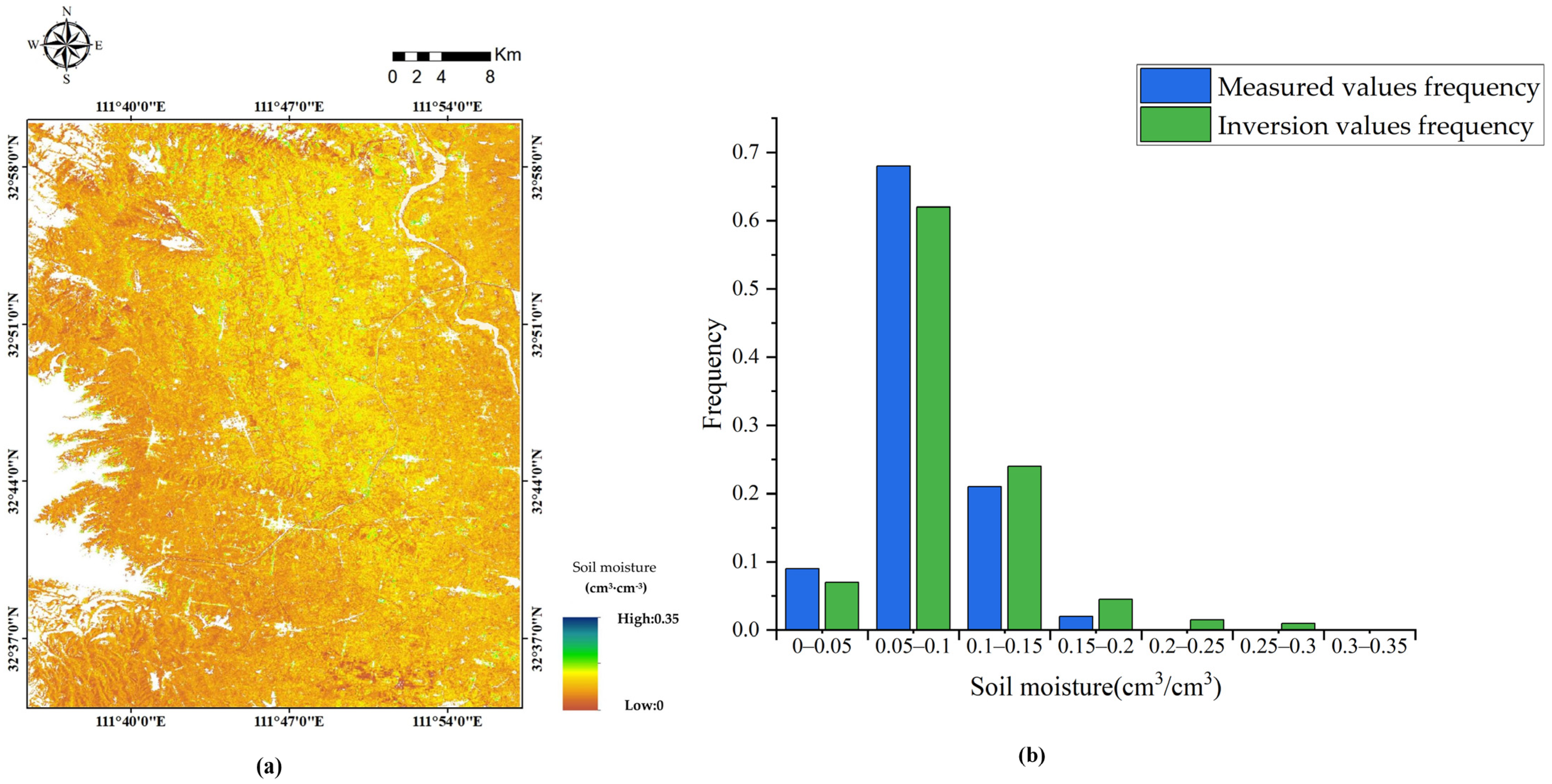
According to the above results, C-band Sentinel-1 data, X-band TerraSAR data, and Sentinel-2 optical remote sensing data were first used. Combined with the optimal parameters of the model obtained by the cross-validation method, the best results were obtained by SSM inversion using the RF model. Therefore, this method was employed in this study to invert the SSM of the study area, obtaining spatial and frequency distribution maps of SSM, as shown in Figure 6 and Figure 7. The non-agricultural areas are filtered out and set to white in the SSM distribution map in order to highlight the agricultural areas.
As shown in Figure 6 and Figure 7, on 23 September 2021, the range distribution of SSM inversion values was primarily between 0.15 and 0.25 cm3/cm3. On 21 December 2021, the inversion values were mainly distributed within the range of 0.05 to 0.1 cm3/cm3. These distributions closely matched the frequency distribution of measured SSM. Additionally, during field measurements in the study area on these two dates, the average SSM values were 0.1864 cm3/cm3 and 0.069 cm3/cm3, respectively. According to the inversion results, the predicted average SSM values for these dates were 0.1839 cm3/cm3 and 0.0726 cm3/cm3, respectively, which closely aligned with the measured SSM values obtained in the field. This indicates that the method exhibited strong applicability in this study area.
In addition, from the SSM spatial distribution maps shown in Figure 6a and Figure 7a, significant differences in SSM between September and December were observed. This phenomenon can be mainly attributed to seasonal variations and the growth cycle of crops. In September, wheat was in the emergence stage, with crops just starting to grow, leading to relatively higher SSM values to meet the growth demands. However, by December, wheat entered the overwintering period, where lower temperatures often caused SSM to condense or freeze, resulting in decreased SSM. Hence, significant differences in SSM between September and December were observed.

4. Discussion

Currently, research on SSM inversion using machine learning methods usually relies on a large amount of measured data. In this study, a new method for SSM inversion by combining multi-band remote sensing data under small sample dataset conditions was proposed. However, there were still some aspects of the applicability and performance of the method that need to be further discussed.

4.1. Analysis of Applicability during Late Vegetation Growth

The SAR remote sensing data used in this study were Sentinel-1 and TerraSAR data, whose wavelengths were 5.6 cm and 3.1 cm, respectively [51]. Their penetration ability was weaker than that of the long-wavelength SAR data in the L-band and P-band. In this study, the wheat in the farmland was in the seedling and overwintering stages. At this time, both the height and vegetation coverage of the wheat were relatively low. During this stage, the wheat plants had not yet formed a dense vegetation canopy, and the soil surface was relatively bare. This allowed the SAR signal to more directly reflect the moisture content of the soil surface. Therefore, better results could be achieved using C-band and X-band Sentinel-1 and TerraSAR data.
However, when the vegetation coverage in the study area was high, the applicability of Sentinel-1 and TerraSAR data significantly decreased. High vegetation coverage led to increased scattering and the attenuation of shorter wavelength radar signals, thus affecting the accuracy and reliability of the data [52]. In such cases, using L-band SAR data with stronger penetration capabilities or optical sensors could yield better results. Due to its longer wavelength, the L-band can more effectively penetrate dense vegetation layers, providing more accurate SSM information.
Therefore, in future research, it is necessary to explore more methods and technological improvements to enhance SSM retrieval accuracy, especially in high-coverage scenarios during the late stages of vegetation growth. Additionally, optimizing the preprocessing and retrieval algorithms for SAR data and further improving the integrated utilization efficiency of different wavelength data are key steps to improving retrieval accuracy.

4.2. Analysis of the Effectiveness of Model Parameters

The influence of machine learning model parameters on performance is crucial. Traditional parameter tuning methods often require a large amount of data for validation [36,37]. But in small sample datasets, the scarcity of data can lead to unstable tuning results. Therefore, a combined approach of cross-validation was adopted in this study to fully utilize the information in small sample datasets, thereby effectively adjusting model parameters. Furthermore, combining cross-validation also enhanced the model’s generalization ability, enabling the model to achieve better performance on small sample datasets.
However, determining whether the final parameters obtained through this method achieved optimal performance in the model still posed certain challenges. This is because parameter selection during the cross-validation process is typically based on a limited number of data subsets, which may not fully represent the feature distribution of the entire dataset. Therefore, further validation and optimization are still necessary when determining the best parameters. Additionally, the choice of the number of folds and the data splitting method in cross-validation can also affect the results of final parameter tuning.
Therefore, in future research, it is necessary to pay more attention to determining the optimal values of model parameters and selecting the most suitable number of folds in cross-validation methods.

5. Conclusions

An SSM inversion method using small sample datasets was proposed to invert farmland SSM based on Sentinel-1, TerraSAR, and Sentinel-2 remote sensing data and GA-BP, SVR, and RF machine learning models. The main conclusions are as follows:
(1) By combining C-band and X-band SAR data with optical data for SSM inversion, it was found that no matter which one of these three machine learning models was used to invert SSM, the inversion results of using C-band and X-band SAR data together with optical data were better than using single SAR data with optical data in the study area.
(2) After optimizing the parameters of the GA-BP, SVR, and RF models using the cross-validation method, all three machine learning models achieved better performance. Among them, the RF model performed best in SSM inversion using small sample datasets, with an R2 of 0.9186, an RMSE of 0.0153 cm3/cm3, and an MAE of 0.0122 cm3/cm3.
The proposed method provides a meaningful reference for SSM inversion using multi-band SAR and optical remote sensing data, particularly in the case of small-sample datasets. In future studies, more machine learning models and parameter optimizing methods could be considered to further improve the SSM inversion performance based on small sample datasets, and the applicability and effectiveness of the proposed method need to be validated and explored in other study areas.

Author Contributions

Methodology, C.X., Q.L., Y.W., Q.C., X.S., H.Z., J.Z. and N.L.; investigation, C.X. and X.S.; experiment and visualization, C.X. and X.S.; validation, Q.L., Y.W., Q.C., H.Z., J.Z. and N.L.; writing—original draft, C.X. and X.S.; writing—review and editing, C.X., Q.L., Y.W., Q.C., X.S., H.Z., J.Z. and N.L. All authors have read and agreed to the published version of the manuscript.

Funding

This work was supported by the National Key Research and Development Program of China under grant (2022YFB3902200) and the Plan of Science and Technology of Henan Province (242102210113).

Data Availability Statement

The original contributions presented in the study are included in the article, further inquiries can be directed to the corresponding author.

Acknowledgments

The authors would like to thank the anonymous reviewers for their valuable and detailed comments, which were crucial in improving the quality of this paper.

Conflicts of Interest

The authors declare no conflicts of interest.

References

  1. Wang, H.; Magagi, R.; Goïta, K. Potential of a two-component polarimetric decomposition at C-band for soil moisture retrieval over agricultural fields. Remote Sens. Environ. 2018, 217, 38–51. [Google Scholar] [CrossRef]
  2. Zhang, L.; Wang, R.; Chai, H.; Lv, X. A polarimetric decomposition and copula quantile regression approach for soil moisture estimation from Radarsat-2 data over vegetated areas. IEEE J. Sel. Top. Appl. Earth Obs. Remote Sens. 2023, 16, 3405–3417. [Google Scholar] [CrossRef]
  3. Brocca, L.; Tarpanelli, A.; Filippucci, P.; Dorigo, W.; Zaussinger, F.; Gruber, A.; Fernández-Prieto, D. How much water is used for irrigation? A new approach exploiting coarse resolution satellite soil moisture products. Int. J. Appl. Earth Obs. Geoinf. 2018, 73, 752–766. [Google Scholar] [CrossRef]
  4. Zohaib, M.; Kim, H.; Choi, M. Detecting global irrigated areas by using satellite and reanalysis products. Sci. Total Environ. 2019, 677, 679–691. [Google Scholar] [CrossRef] [PubMed]
  5. Zohaib, M.; Choi, M. Satellite-based global-scale irrigation water use and its contemporary trends. Sci. Total Environ. 2020, 714, 136719. [Google Scholar] [CrossRef]
  6. Zhao, J.; Zhang, C.; Min, L.; Guo, Z.; Li, N. Retrieval of farmland surface soil moisture based on feature optimization and machine learning. Remote Sens. 2022, 14, 5102. [Google Scholar] [CrossRef]
  7. Wang, S.N.; Li, R.P.; Wu, Y.J.; Zhao, S.X.; Wang, X.Q. Soil moisture inversion based on environmental variables and machine learning. J. Agric. Mach. 2022, 53, 332–341. [Google Scholar]
  8. Ma, H.Z.; Liu, S.M.; Peng, A.H.; Sun, L.; Sun, G.Y. Active and passive cooperative algorithm at L-Band for bare soil moisture inversion. Trans. Chin. Soc. Agric. Eng. 2016, 32, 133–138. [Google Scholar]
  9. Wang, S.G.; Ma, C.F.; Zhao, Z.B.; Wei, L. Estimation of Soil Moisture of Agriculture Field in the Middle Reaches of the Heihe River Basin based on Sentinel-1 and Landsat 8 Imagery. Remote Sens. Technol. Appl. 2020, 35, 13–22. [Google Scholar]
  10. Wang, Y.T. Remote Sensing Retrieval of Soil Moisture in Ordos Blown-Sand Region Based on SVR. Master’s Thesis, Chang’an University, Xi’an, China, 2019. [Google Scholar]
  11. Liu, D.; Mishra, A.K.; Yu, Z. Evaluating uncertainties in multi-layer soil moisture estimation with support vector machines and ensemble Kalman filtering. J. Hydrol. 2016, 538, 243–255. [Google Scholar] [CrossRef]
  12. De Roo, R.D.; Du, Y.; Ulaby, F.T.; Dobson, M.C. A semi-empirical backscattering model at L-band and C-band for a soybean canopy with soil moisture inversion. IEEE Trans. Geosci. Remote Sens. 2001, 39, 864–872. [Google Scholar] [CrossRef]
  13. Verhoest, N.E.; Lievens, H.; Wagner, W.; Álvarez-Mozos, J.; Moran, M.S.; Mattia, F. On the soil roughness parameterization problem in soil moisture retrieval of bare surfaces from synthetic aperture radar. Sensors 2008, 8, 4213–4248. [Google Scholar] [CrossRef] [PubMed]
  14. Marzahn, P.; Ludwig, R. On the derivation of soil surface roughness from multi parametric PolSAR data and its potential for hydrological modeling. Hydrol. Earth Syst. Sci. 2009, 13, 381–394. [Google Scholar] [CrossRef]
  15. Liu, Q.; Wu, Z.; Cui, N.; Jin, X.; Zhu, S.; Jiang, S.; Zhao, L.; Gong, D. Estimation of Soil Moisture Using Multi-Source Remote Sensing and Machine Learning Algorithms in Farming Land of Northern China. Remote Sens. 2023, 15, 4214. [Google Scholar] [CrossRef]
  16. Wang, R.; Zhao, J.; Yang, H.; Li, N. Inversion of Soil Moisture on Farmland Areas Based on SSA-CNN Using Multi-Source Remote Sensing Data. Remote Sens. 2023, 15, 2515. [Google Scholar] [CrossRef]
  17. Leng, P.; Li, Z.L.; Duan, S.B.; Gao, M.F.; Huo, H.Y. A Practical Approach for Deriving All-Weather Soil Moisture Content Using Combined Satellite and Meteorological Data. ISPRS J. Photogrammetry Remote Sens. 2017, 131, 40–51. [Google Scholar] [CrossRef]
  18. Al-Yaari, A.; Wigneron, J.P.; Ducharne, A.; Kerr, Y.; De Rosnay, P.; De Jeu, R.; Mialon, A. Global-scale evaluation of two satellite-based passive microwave soil moisture datasets (SMOS and AMSR-E) with respect to Land Data Assimilation System estimates. Remote Sens. Environ. 2014, 149, 181–195. [Google Scholar] [CrossRef]
  19. Liu, J.; Xu, Y.; Li, H.; Guo, J. Soil Moisture Retrieval in Farmland Areas with Sentinel Multi-Source Data Based on Regression Convolutional Neural Networks. Sensors 2021, 21, 877. [Google Scholar] [CrossRef] [PubMed]
  20. Ma, C.; Li, X.; McCabe, M.F. Retrieval of High-Resolution Soil Moisture through Combination of Sentinel-1 and Sentinel-2 Data. Remote Sens. 2020, 12, 2303. [Google Scholar] [CrossRef]
  21. Liu, Y.; Qian, J.; Yue, H. Combined Sentinel-1A with Sentinel-2A to estimate soil moisture in farmland. IEEE J. Sel. Top. Appl. Earth Obs. Remote Sens. 2020, 14, 1292–1310. [Google Scholar] [CrossRef]
  22. Zhang, X.; Chen, B.; Fan, H.; Huang, J.; Zhao, H. The Potential Use of Multi-Band SAR Data for Soil Moisture Retrieval over Bare Agricultural Areas: Hebei, China. Remote Sens. 2016, 8, 7. [Google Scholar] [CrossRef]
  23. Yadav, V.P.; Prasad, R.; Bala, R.; Vishwakarma, A.K. An improved inversion algorithm for spatio-temporal retrieval of soil moisture through modified water cloud model using C-band Sentinel-1A SAR data. Comput. Electron. Agric. 2020, 173, 105447. [Google Scholar] [CrossRef]
  24. Jing, L.; Yang, L.; Yang, W.; Xu, T.; Gao, F.; Lu, Y.; Sun, B.; Yang, D.; Hong, X.; Wang, N.; et al. Robust Kalman Filter Soil Moisture Inversion Model Using GPS SNR Data—A Dual-Band Data Fusion Approach. Remote Sens. 2021, 13, 4013. [Google Scholar] [CrossRef]
  25. Naidoo, L.; Mathieu, R.; Main, R.; Kleynhans, W.; Wessels, K.; Asner, G.; Leblon, B. Savannah woody structure modelling and map** using multi-frequency (X-, C-and L-band) Synthetic Aperture Radar data. ISPRS J. Photogrammetry Remote Sens. 2015, 105, 234–250. [Google Scholar] [CrossRef]
  26. Lee, S.-J.; Choi, C.; Kim, J.; Choi, M.; Cho, J.; Lee, Y. Estimation of High-Resolution Soil Moisture in Canadian Croplands Using Deep Neural Network with Sentinel-1 and Sentinel-2 Images. Remote Sens. 2023, 15, 4063. [Google Scholar] [CrossRef]
  27. Zhang, L.; Zhang, Z.; Xue, Z.; Li, H. Sensitive Feature Evaluation for Soil Moisture Retrieval Based on Multi-Source Remote Sensing Data with Few In-Situ Measurements: A Case Study of the Continental US. Water 2021, 13, 2003. [Google Scholar] [CrossRef]
  28. Wang, J.; Wu, F.; Shang, J.; Zhou, Q.; Ahmad, I.; Zhou, G. Saline soil moisture mapping using Sentinel-1A synthetic aperture radar data and machine learning algorithms in humid region of China’s east coast. Catena 2022, 213, 106189. [Google Scholar] [CrossRef]
  29. Du, H.; Li, M.; Xu, Y.; Zhou, C. An ensemble learning approach for land use/land cover classification of arid regions for climate simulation: A case study of Xinjiang, Northwest China. IEEE J. Sel. Top. Appl. Earth Obs. Remote Sens. 2023, 16, 2413–2426. [Google Scholar] [CrossRef]
  30. Ahmad, S.; Kalra, A.; Stephen, H. Estimating soil moisture using remote sensing data: A machine learning approach. Adv. Water Resour. 2010, 33, 69–80. [Google Scholar] [CrossRef]
  31. Ulaby, F.T.; Moore, R.K.; Fung, A.K. Microwave Remote Sensing: Active and Passive. Volume 2-Radar Remote Sensing and Surface Scattering and Emission Theory; NASA: Washington, DC, USA, 1982. [Google Scholar]
  32. Tao, L.; Li, J.; Jiang, J.; Chen, X.; Cai, Q. A modified vegetation backscattering model for leaf area index retrieval from SAR time series. Int. J. Remote Sens. 2016, 37, 5884–5901. [Google Scholar] [CrossRef]
  33. Baghdadi, N.N.; El Hajj, M.; Zribi, M.; Fayad, I. Coupling SAR C-band and optical data for soil moisture and leaf area index retrieval over irrigated grasslands. IEEE J. Sel. Top. Appl. Earth Observ. Remote Sens. 2015, 9, 1229–1243. [Google Scholar] [CrossRef]
  34. Balenzano, A.; Mattia, F.; Satalino, G.; Davidson, M.W.J. Dense temporal series of C-and L-band SAR data for soil moisture retrieval over agricultural crops. IEEE J. Sel. Top. Appl. Earth Obs. Remote Sens. 2010, 4, 439–450. [Google Scholar] [CrossRef]
  35. Kseneman, M.; Gleich, D. Soil-moisture estimation from X-band data using Tikhonov regularization and neural net. IEEE Trans. Geosci. Remote Sens. 2013, 51, 3885–3898. [Google Scholar] [CrossRef]
  36. Zhu, L.; Dai, J.; Liu, Y.; Yuan, S.; Qin, T.; Walker, J.P. A cross-resolution transfer learning approach for soil moisture retrieval from Sentinel-1 using limited training samples. Remote Sens. Environ. 2024, 301, 113944. [Google Scholar] [CrossRef]
  37. Xu, W.; Zhang, Z.; Qin, Q.; Hui, J.; Long, Z. Soil moisture estimation with SVR and data augmentation based on alpha approximation method. IEEE Trans. Geosci. Remote Sens. 2019, 58, 3190–3201. [Google Scholar] [CrossRef]
  38. Chen, L.; Xing, M.; He, B.; Wang, J.; Shang, J.; Huang, X.; Xu, M. Estimating soil moisture over winter wheat fields during growing season using machine-learning methods. IEEE J. Sel. Top. Appl. Earth Obs. Remote Sens. 2021, 14, 3706–3718. [Google Scholar] [CrossRef]
  39. Ai, P.; Xiong, C.; Li, K.; Song, Y.; Gong, S.; Yue, Z. Effect of Data Characteristics Inconsistency on Medium and Long-Term Runoff Forecasting by Machine Learning. IEEE Access. 2023, 11, 11601–11612. [Google Scholar] [CrossRef]
  40. Tang, T.; Jiao, D.; Chen, T.; Gui, G. Medium-and long-term precipitation forecasting method based on data augmentation and machine learning algorithms. IEEE J. Sel. Top. Appl. Earth Obs. Remote Sens. 2022, 15, 1000–1011. [Google Scholar] [CrossRef]
  41. Li, S.; Ye, C.; Zhang, Q. 11-Year change in water chemistry of large freshwater Reservoir Danjiangkou, China. J. Hydrol. 2017, 551, 508–517. [Google Scholar] [CrossRef]
  42. Wu, S.; Yang, P.; Ren, J.; Chen, Z.; Liu, C.; Li, H. Winter wheat LAI inversion considering morphological characteristics at different growth stages coupled with microwave scattering model and canopy simulation model. Remote Sens. Environ. 2020, 240, 111681. [Google Scholar] [CrossRef]
  43. Chen, J.; Lin, H.; Huang, C.; Fang, C. The relationship between the leaf area index (LAI) of rice and the C-band SAR vertical/horizontal (VV/HH) polarization ratio. Int. J. Remote Sens. 2009, 30, 2149–2154. [Google Scholar] [CrossRef]
  44. Huang, X.; Wang, J.; Shang, J.; Liao, C.; Liu, J. Application of polarization signature to land cover scattering mechanism analysis and classification using multi-temporal C-band polarimetric RADARSAT-2 imagery. Remote Sens. Environ. 2017, 193, 11–28. [Google Scholar] [CrossRef]
  45. Qi, J.; Chehbouni, A.; Huete, A.R.; Kerr, Y.H.; Sorooshian, S. A modified soil adjusted vegetation index. Remote Sens. Environ. 1994, 48, 119–126. [Google Scholar] [CrossRef]
  46. Bao, Y.; Lin, L.; Wu, S.; Deng, K.A.; Petropoulos, G.P. Surface soil moisture retrievals over partially vegetated areas from the synergy of Sentinel-1 and Landsat 8 data using a modified water-cloud model. Int. J. Appl. Earth Obs. Geoinf. 2018, 72, 76–85. [Google Scholar] [CrossRef]
  47. Li, Z.; Yuan, Q.; Zhang, L. Geo-intelligent retrieval framework based on machine learning in the cloud environment: A case study of soil moisture retrieval. IEEE Trans. Geosci. Remote Sens. 2023, 61, 1–15. [Google Scholar] [CrossRef]
  48. Liu, D.; Liu, C.; Tang, Y.; Gong, C. A GA-BP Neural Network Regression Model for Predicting Soil Moisture in Slope Ecological Protection. Sustainability 2022, 14, 1386. [Google Scholar] [CrossRef]
  49. Brereton, R.G.; Lloyd, G.R. Support vector machines for classification and regression. Analyst 2010, 135, 230–267. [Google Scholar] [CrossRef]
  50. Lyu, Z.; Yu, Y.; Samali, B.; Rashidi, M.; Mohammadi, M.; Nguyen, T.N.; Nguyen, A. Back-Propagation Neural Network Optimized by K-Fold Cross-Validation for Prediction of Torsional Strength of Reinforced Concrete Beam. Materials 2022, 15, 1477. [Google Scholar] [CrossRef]
  51. Pasternak, M.; Pawłuszek-Filipiak, K. Evaluation of C and X-Band Synthetic Aperture Radar Derivatives for Tracking Crop Phenological Development. Remote Sens. 2023, 15, 4996. [Google Scholar] [CrossRef]
  52. Cheng, M.; Jiao, X.; Liu, Y.; Shao, M.; Yu, X.; Bai, Y.; Wang, Z.; Wang, S.; Tuohuti, N.; Liu, S.; et al. Estimation of soil moisture content under high maize canopy coverage from UAV multimodal data and machine learning. Agric. Water Manag. 2022, 264, 107530. [Google Scholar] [CrossRef]
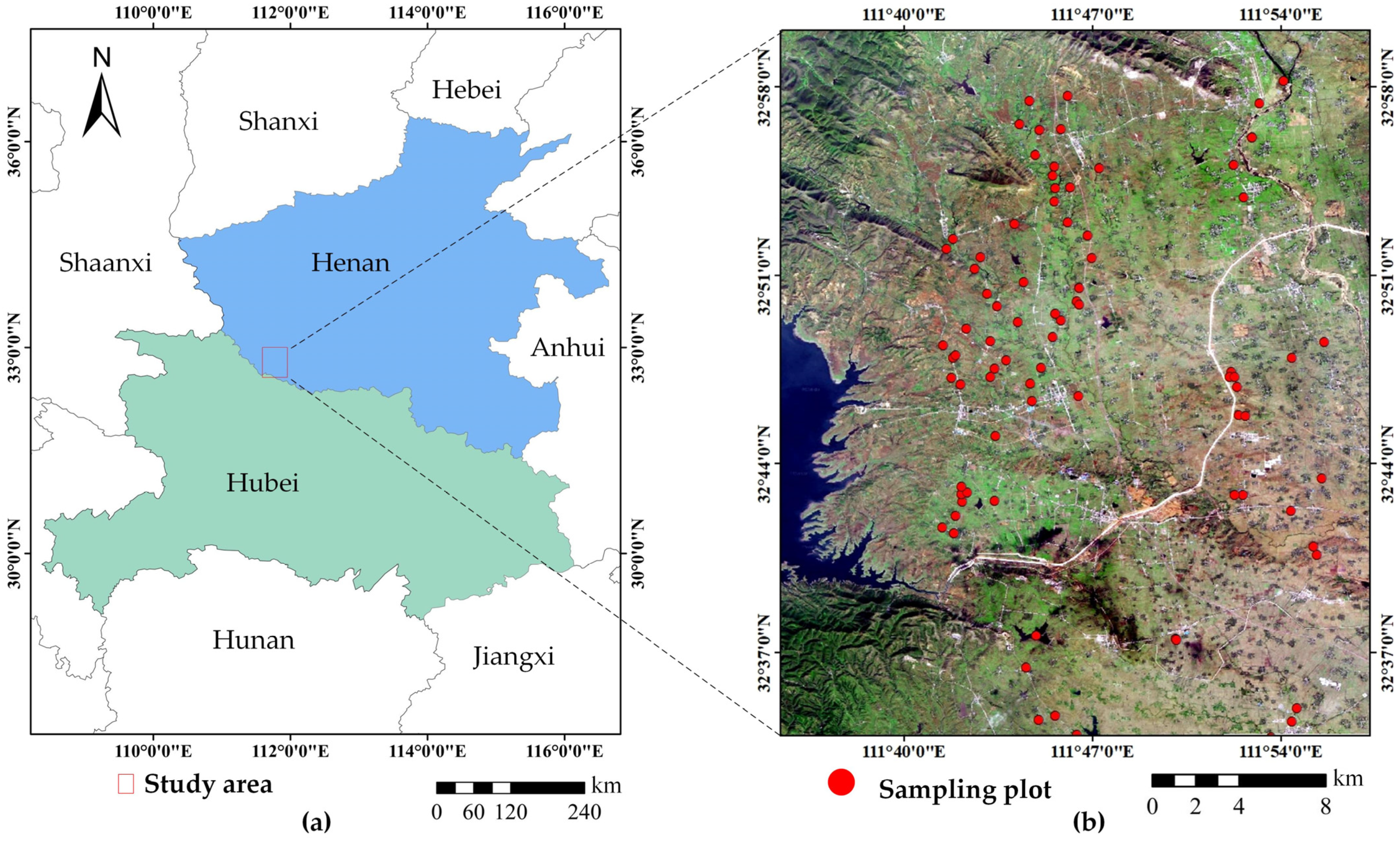
Figure 1. Location of the study area and sampling sites: (a) geographical location of the study area; (b) study area and sampling plot.
Remotesensing 16 02296 g001
Figure 2. Technology roadmap.
Remotesensing 16 02296 g002
Figure 3. The 10-fold cross-validation model selection chart.
Remotesensing 16 02296 g003
Figure 4. Comparison of accuracy of different data combinations on the training set: (a) differences in R2; (b) differences in RMSE; and (c) differences in MAE.
Remotesensing 16 02296 g004
Figure 5. Comparison of the accuracy of different machine learning models on the training set and validation set: (a) differences in R2; (b) differences in RMSE; and (c) differences in MAE.
Remotesensing 16 02296 g005
Figure 6. Results of SSM inversion in the study area on 23 September 2021: (a) spatial distribution of inverted SSM; (b) frequency distribution of inverted and measured SSM.
Remotesensing 16 02296 g006
Figure 7. Results of SSM inversion in the study area on 21 December 2021: (a) spatial distribution of inverted SSM; (b) frequency distribution of inverted and measured SSM.
Remotesensing 16 02296 g007
Table 1. Remote sensing data information.
Data SourceAcquisition DateBandSpatial ResolutionTemporal
Resolution
Product TypePolarization Mode
Sentinel-123 September 2021C10 m12 dIWVV/VH
16 December 2021
TerraSAR24 September 2021X18 m11 dScanSARHH
21 December 2021
Sentinel-222 September 2021
21 December 2021
Band 160 m10 dL2A-
Band 210 m
Band 310 m
Band 410 m
Band 520 m
Band 620 m
Band 720 m
Band 810 m
Band 8A20 m
Band 960 m
Band 1060 m
Band 1120 m
Band 1220 m
Ground observation data23 September 2021-----
21 December 2021
Table 2. Extracted feature parameters.
No.ParameterNote
1 θ Sentinel-1 incident angle
2 V V VV backscatter coefficients
3 V H VH backscatter coefficients
4 H H HH backscatter coefficients
5NDVINormalized Difference Vegetation Index
6NDWINormalized Difference Water Index
Table 3. Multi-band data combinations.
No.Data TypeData
1C-Band + OpticalSentinel-1 + Sentinel-2
2X-Band + OpticalTerraSAR-X + Sentinel-2
3C-Band+X-Band + OpticalSentinel-1 + TerraSAR-X + Sentinel-2
Table 4. SSM inversion accuracy comparison of different data combinations on the test set.
Machine
Learning Model
Input Data SourceR2RMSE
(cm3/cm3)
MAE
(cm3/cm3)
GA-BPSentinel-1 + Sentinel-20.62860.02820.0281
TerraSAR-X + Sentinel-20.67190.02410.0265
Sentinel-1 + TerraSAR-X + Sentinel-20.72080.0370.0309
SVRSentinel-1 + Sentinel-20.68220.02540.0269
TerraSAR-X + Sentinel-20.71260.02350.0292
Sentinel-1 + TerraSAR-X + Sentinel-20.79840.03040.0276
RFSentinel-1 + Sentinel-20.75350.01920.0134
TerraSAR-X + Sentinel-20.83060.01900.0144
Sentinel-1 + TerraSAR-X + Sentinel-20.88120.01690.0131
Table 5. Parameter values for different models.
Machine
Learning Model
ParameterParameter Value
before Selection
Parameter
Value
GA-BPHidden Layers11
Number of nodes109
Population size10050
Number of iterations100100
SVRPenalty parameter56
Kernel function coefficients0.50.1
RFNumber of trees50100
Maximum depth of the tree105
Table 6. Comparison of inversion results of different models on the test set.
Machine
Learning Model
R2RMSE
(cm3/cm3)
MAE
(cm3/cm3)
GA-BP0.73460.03570.0276
SVR0.82470.02790.0218
RF0.91860.01530.0122
Disclaimer/Publisher’s Note: The statements, opinions and data contained in all publications are solely those of the individual author(s) and contributor(s) and not of MDPI and/or the editor(s). MDPI and/or the editor(s) disclaim responsibility for any injury to people or property resulting from any ideas, methods, instructions or products referred to in the content.