Article

Assessment of Adjacency Correction over Inland Waters Using Sentinel-2 MSI Images

1
Earth Observation and Geoinformatics Division, National Institute for Space Research, São José dos Campos 12227-010, SP, Brazil
2
Instrumentation Laboratory for Aquatic Systems (LabISA), Earth Observation Coordination of National Institute for Space Research (INPE), São José dos Campos 12227-010, SP, Brazil
3
Department of Agricultural & Biological Engineering, Mississippi State University, Starkville, MS 39762, USA
4
Departamento de Meteorologia, Universidade do Rio de Janeiro (UFRJ), Rio de Janeiro 21941-916, RJ, Brazil
*
Author to whom correspondence should be addressed.
Remote Sens. 2022, 14(8), 1829; https://doi.org/10.3390/rs14081829
Submission received: 24 February 2022 / Revised: 2 April 2022 / Accepted: 4 April 2022 / Published: 11 April 2022
(This article belongs to the Special Issue Advances in Remote Sensing of the Inland and Coastal Water Zones)

Abstract

:
Satellite remote sensing data have been used for water quality mapping, but accurate water reflectance retrieval is dependent on multiple procedures, such as atmospheric and adjacency corrections. For the latter, physical-based methods are used to minimize the adjacency effects caused by neighboring land targets close to water pixels, and implementation requires atmospheric and environmental parameters, such as aerosol optical depth and horizontal range (i.e., distance in meters) of the adjacency effect ( H Adj ). Generally, the H Adj is empirically defined by users and can lead to substantial errors in water reflectance when incorrectly used. In this research, a physical-based approach with three empirical methods to determine the H Adj (fixed, SIMilarity Environment Correction—SIMEC, and Adaptative Window by Proportion—AWP-Inland Water) were used to correct and characterize the adjacency effects in Sentinel-2 images over Brazilian inland waters. An interactive inversion method of the deep blue waveband estimated the aerosol loading for the atmospheric correction procedure. The results of atmospheric and adjacency corrections were validated against in-situ reflectance data. The inverted aerosol loading achieved a good agreement with in-situ measurements, especially at visible wavelengths (Mean Absolute Percentage Error—MAPE for eutrophic (~56%), bright (~80%), and dark (~288%) waters). The adjacency correction performance was near similar between the SIMEC and AWP-Inland Water methods in eutrophic and bright waters (MAPE difference < 3%). However, only the AWP-Inland Water method provided a smaller error (MAPE ~53%) for dark waters compared to the fixed (~108%) and SIMEC (~289%) methods, which shows how critical H Adj parametrization is for low water reflectance values. Simulations of different atmospheric and adjacency effects were performed, and they highlighted the importance of adjacency correction under aerosol loading higher 0.1, which is a typical aerosol loading in a dry climate season, and over extremely dark, low-reflectance waters. This paper contributes to further understanding adjacency effects in medium spatial resolution imagery of inland waters using a physical-based approach including the uncertainties in H Adj determination.

Graphical Abstract

1. Introduction

Inland waters are essential ecosystems for life on Earth [1]. They are sources of drinking water, socio-economic services (e.g., power generation, fisheries, recreation, and irrigation), and ecosystem services (e.g., biodiversity maintenance) [2]. By 2050, scientific projections indicate that most of the world’s population (*52%) will be living in water-stressed areas [3], predicting that water demand will surpass its availability in the following decades. Thus, monitoring these environments is crucial to ensure water availability for its multiple uses. Biophysical monitoring of inland waters at large space–time scales is only feasible with satellite remote sensing data sources. The advance of new satellite sensors with better radiometric quality and higher spectral, spatial, and temporal resolutions, such as Landsat-8 OLI and Sentinel-2 MSI [4,5,6,7], has sparked the water remote sensing community’s interest in using these systems for the mapping of inland waters’ Optically Active Components—OACs [8,9,10,11]. However, atmospheric and adjacency effect corrections [12] are still a challenge in achieving accurate water reflectance estimates for high- and medium-resolution satellite imagery.
The adjacency effect is caused by reflected photons from surrounding land targets that are scattered by atmosphere components into the sensor’s field of view [13,14,15]. This complex phenomenon reduces the contrast between the high-reflectivity (land) and the low-reflectivity (water) surfaces. As a result, scattered photons from the land targets close to the water bodies can distort water spectral reflectance, mainly affecting small water bodies [12]. The magnitude of these effects depends on several factors, such as atmosphere composition (e.g., aerosol particle properties), land-cover type, viewing and illumination geometry, sensor characteristics (e.g., spatial resolution), and the shape and size of water bodies [16,17,18]. When neglected, the adjacency effect can introduce significant errors in retrieving the water-leaving signal [19], limiting the use of satellite imagery for estimating OACs.
Adjacency correction in satellite imagery uses physical approaches that allow the application of radiative transfer theory and Atmospheric Point Spread Function—APSF to quantify and remove the adjacency effects [15,20,21]. In this context, APSF describes the contribution of reflected photons from the neighboring targets into the interest target [22,23]. Tanré et al. [15] and Vermote et al. [21] have suggested a robust formulation for APSF recovery based on Monte Carlo simulations, where the APSF results from the contribution of molecular (or Rayleigh) and aerosol scattering. The inherent challenge in applying this method is estimating the range of the adjacency effect ( H Adj ), which refers to the maximum extent of the adjacency effects around the interest target, because it depends on often unknown factors [24]. Alternatively, the H Adj has been chosen arbitrarily [25,26] or defined iteratively by comparing the corrected image reflectance with the spectral responses of targets [18,27,28]. An improper choice of H Adj can lead to over- or under-correction of water reflectance due to the mischaracterization of environmental conditions around the water target.
Few studies have assessed the accuracy of the correction of adjacency effects on water reflectance [12,29,30]. The methodology complexity and limited open-source software for adjacency effect correction can partially explain this lacune. In this way, the assessment of water reflectance products has been generally performed in terms of (i) intercomparison between different atmospheric correction methods assuming a uniform surface (i.e., without adjacent correction) [31,32], (ii) validation of adjacency effects for large lakes (surface area greater than 370 km2) or coastal waters [29,33], or (iii) theoretical water reflectance simulations for a variety of atmospheric conditions and coastal water types [16,17,34]. Over inland waters, adjacency effects are under-discussed, and a recent study showed the importance of correcting adjacency problems when estimating OACs in these environments [19]. For this reason, a physical-based method to fix adjacency effects with a practical empirical assumption for H Adj estimation remains necessary research for inland waters.
This study explores the adjacency effects over Brazilian inland waters in medium spatial resolution Sentinel-2 (A and B) MSI images. The paper’s focus is to assess the satellite imagery reflectance uncertainties caused by adjacency effects using a physical-based approach [15,21] on small lakes surrounded by dense forest cover and on a large water urban reservoir considering variable aerosol loadings. Our assessment of satellite-derived water reflectance contributes to understanding (i) the effect of optical water types on adjacency correction, (ii) the performance of a physical method in complex environments (e.g., atmospheric scattering conditions and shape and size of water bodies), (iii) the proper definition of the size of the H Adj , (iv) the impact of external factors on modeling the adjacency effect for inland waters, and (v) the conditions under which this effect is negligible. Here, we analyze two different methods to retrieve the H Adj : (i) considering the size of the H Adj constant along the water body (hereafter called fixed), and (ii) varying the H Adj pixel-by-pixel (hereafter called adaptive). The adaptive methods tested were SIMilarity Environment Correction—SIMEC [33] and Adaptative Window by Proportion applied to Inland Water—AWP-Inland Water. AWP-Inland Water is a proto-algorithm developed in this study based on the proportion of non-water targets within the window. The atmospheric and adjacency correction validation used field data acquired in a time interval close to the satellite overpasses. Moreover, this study further investigates the magnitude of the adjacency effect using the Second Simulation of a Satellite Signal in the Solar Spectrum (6SV) to simulate its impact under different water optical types, aerosol properties (e.g., aerosol loading and model), and land-cover types.

2. Materials and Methods
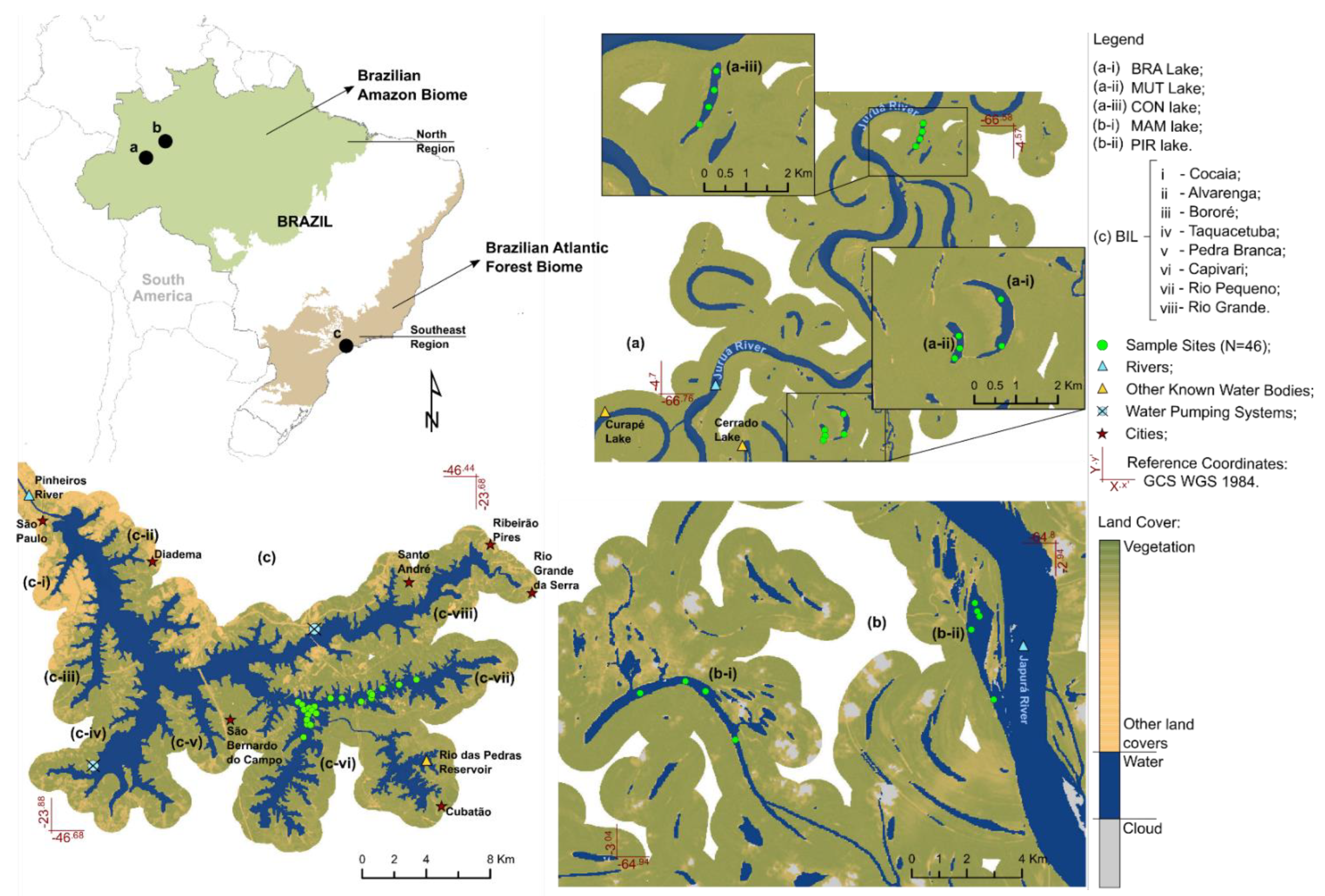
2.1. Study Area

Five small lakes (Mamirauá—MAM, Pirarara—PIR, Concordia—CON, Branco—BRA, and Mutum—MUT) and one large reservoir (Billings—BIL) were selected for the analysis (Figure 1). These water bodies represent different sceneries regarding land cover, shape and size, and optically active water components in Brazil’s north and southeast regions. Billings reservoir (127 km2) is one of the largest water systems in the metropolitan region of São Paulo State, serving multiple purposes including public water supply, energy generation, fisheries, and recreation [35,36]. Frequent algae blooms and potentially toxic cyanobacteria dominate Billings’ optical properties and impair its water quality [35,37,38,39]. The reservoir is divided into eight narrow arms that contribute to a broader and elongated central body [36]. In general, the arms’ average width is approximately 500 m, but sometimes it is smaller than 100 m. These narrow arms and the proximity to urban targets make the Billings reservoir a suitable study site to investigate the adjacency effect.
The other selected water bodies encompass Amazon floodplain lakes with surface areas smaller than 3 km2. Two of them, Mamirauá and Pirarara, are located inside the Mamirauá Sustainable Development Reserve—MSDR close to the confluence of the Solimões and Japurá rivers. The remaining three lakes, Concordia, Branco, and Mutum, belong to the Juruá River floodplain. These lakes are located in well-preserved areas under low human influence and are surrounded by a dense flooded forest cover. The water flow exchange with the fluvial systems [40] and the land coverage around the lakes [41] strongly influence the bio-optical compositions of these ecosystems. For example, Pirarara lake has brighter waters because it is connected to the Japurá River and receives a high inflow from its temporarily sediment-laden waters. Four of these lakes have dark waters with reflectance values smaller than 4%. In these cases, they are perennial lakes and suffer influence from the surrounding forest, which during the rising and flooding season, washes into the lakes large amounts of dissolved organic matter accumulated year-round [41,42].
The water bodies chosen in this study are potential environments for bio-optical modeling applied to the water quality monitoring of urban reservoirs and sustainable management of small lakes using remote sensing data [10,37,43]. For that reason, the investigation of factors that influence the accurate recovery of OACs, including the adjacency effect, becomes essential in these regions.

2.2. Dataset

2.2.1. MSI/Sentinel-2 Data

Multi-Spectral Instrument—MSI sensors onboard Sentinel-2 (A and B) satellites were used to assess adjacency effect correction in this study. The MSI Earth observation data are acquired with fine spatial resolution (10, 20, and 60 m depending on the band) and radiometric resolution (12-bit) in 13 spectral bands localized in the visible near-infrared and short-wave-infrared regions. The Sentinel-2 mission consists of two satellites that carry identical sensors that allow a revisit time of five days at the equator [44]. Although this instrument did not aim at remote sensing aquatic environments, it has accurately performed inland water applications [8,10,45]. Additionally, it increases the possibility for monitoring small water bodies (area smaller than 0.002 km2; see [46]). In addition to water quality monitoring applications, the MSI configuration also helps to investigate the adjacency effect, since: (i) on surfaces with high-contrast among land covers (e.g., water and earth interface), the contamination of the spectral information may be more disrupting in images of medium- and high-spatial resolution; (ii) there is a trend of the adjacency effect to be greater in small and narrow water bodies; and (iii) the increase in time-frequency of image acquisition enables a more significant number of field samplings concurrent to satellite overpass, increasing the number of samples for calibration and validation of the satellite sensor’s measurements.
Images were acquired over the water body regions on 27 August 2017 (MAM and PIR), 20 August 2019 (CON, BRA, and MUT), and 9 August 2021 (BIL). The scenes were downloaded from the Copernicus Open Access Hub website (https://scihub.copernicus.eu/) as L1C products that were corrected for radiometric and geometric distortions with pixel values referring to Top of Atmosphere—TOA reflectance [47]. The selected images had less than 10% cloud cover and cloud-free conditions over all the field sampling sites (Section 2.2.2). After that, the atmosphere and adjacency effect corrections were applied to the TOA reflectance data. Details are discussed in Section 2.4. and Section 2.5.

2.2.2. Field Data

This study used in-situ radiometric data collected to validate MSI surface reflectance imagery after atmospheric and adjacency corrections. Field campaigns in the water bodies occurred during 25–28 August 2017 (MAM and PIR), 19–20 August 2019 (CON, BRA, and MUT), and 8–9 August 2021 (BIL). The time difference between the in-situ reflectance measurements and satellite images can reduce the data correlation due to water composition variability [48,49]. Therefore, we used a time window of ±48 h for the match-up analysis. Over inland waters, commonly size time windows of 2 h—7 days are applied to validate the atmospheric and adjacency corrections [12,29,31,50]. In addition, we also highlight that the water bodies selected did not present fast changes during the field campaigns because both systems, the reservoir and small lakes, were under conditions that minimized abrupt variations in the optical components of the water in a short period. For instance, Billings reservoir has a hydraulic residence time (392 days) and a maximum depth (18 m) [51] that both decrease the water column turbulence and bottom sediment resuspension. Likewise, the small Amazon floodplain lakes, although their water level and circulation are influenced by the flood pulse, these processes occur gradually throughout the hydrological year [40,52,53] with a minimal influence in short time windows during the rising season in meandering rivers, such as Juruá [54].
A total of 46 in-situ samples from BIL (N = 28) and other lakes (N = 18) were collected. A suitable distance from the water body edge was adopted for all sample sites to avoid or reduce the effect of pixel mixture at the land–water interface, bottom reflectance, and adjacency contamination from the surrounding targets (e.g., forest). The sampling sites were placed on the lakes’ central regions, and at BIL, they were split into two categories: sites placed at distances smaller than 100 m (N = 14) and larger than 100 m (N = 14). Due to BIL’s large area, collecting in-situ samples close to the reservoir’s edge was fundamental to validating the adjacency effect because this problem is much larger near land targets around water bodies [17]. In general, the depth of these sites (>3 m) in comparison with the in-situ Secchi depth (<1 m) measured indicates that shallow water effects did not influence the data collected near the water body’ boundary; that is, this study assumes that these regions are optically deep. We had difficulties sampling throughout BIL due to its extension and the need for feasible illumination conditions during the measurements. Thus, the samples were collected mainly along the Rio Pequeno arm and at the beginning of the Capivari arm (see Figure 1).
At each sample site, the remote sensing reflectance ( R rs ) was estimated using the radiometric quantities obtained by three intercalibrated spectroradiometers (TriOS-RAMSES). All sensors operated simultaneously and measured the total water-leaving radiance ( L t ( λ ,   θ v ,   ϕ v ) ), the downwelling sky radiance ( L sky ( λ ,   θ v ,   ϕ v ) ), and the total irradiance incident on the water surface ( E s ( λ ) ) within 350–950 nm wavelengths (at ~3.3 nm increments). The measurements were performed between 10:00 a.m. and 1:00 p.m., and the sensors were positioned at selected angles to minimize sun glint effects following the recommendations of [55]: with the Sun as a reference, the zenith ( θ v ) and azimuth ( ϕ v ) angles of the L t term were ( 45 ° ,   90 ° 135 ° ) and ( θ v ,   ϕ v ) = ( θ v + 90 ° ,   ϕ v = ϕ v ) for the L sky term. With these data, each radiometric record was resampled at 1 nm, and the spectral R rs was calculated utilizing the following equation:
R rs ( λ ) = L t ( λ , θ v , ϕ v )   Rho sky ( θ v , ϕ v ,   θ 0 , W )   L sky ( λ , θ v , ϕ v ) E s ( λ )   ( sr 1 )
where Rho sky is a coefficient that corrects the skylight reflection effects and depends on the wind speed ( W ), view geometry ( θ v ,   ϕ v ), and Sun zenith angle ( θ 0 ); it can be obtained in [56]. Afterward, the water reflectance ( ρ w ) was obtained by multiplying R rs by the value of π . The ρ w   was used in the simulation of the Sentinel-2 MSI bands (visible to near-infrared) using their Spectral Response Function—SRF to generate multispectral data comparable to the corrected image reflectance values in this study:
ρ w * ( B i ) = a b ρ w ( λ )   ×   SRF ( λ )   d λ a b SRF ( λ )   ( Unitless )  
where ρ w * is the MSI reflectance simulated from in-situ data, B i is the MSI spectral band, [ a ,   b ] is the range of the spectral band, and λ is the wavelength.

2.3. The Selection of Water Types

Water composition affects the shape and magnitude of the spectra (Figure 2). In general, the signals of eutrophic and bright waters are up to ~2 times greater than that of dark waters at visible wavelengths (~400–700 nm), and this difference decreases along the spectrum. When observed by the orbital sensors, water bodies with different optical types present distinct behaviors regarding atmospheric and adjacency noise [5,17,42]. Thus, the grouping of water bodies according to their spectral features helps to understand the adjacency effect on inland waters. In this way, we classified the water bodies into artificial eutrophic urban reservoirs (BIL) and natural lakes surrounded by forest, classifying them afterward into bright- (PIR) and dark- (MAM, CON, BRA, and MUT) water lakes, following the criteria defined in [12]. They are named eutrophic, bright, and dark waters throughout this study. It is essential to highlight that the water bodies inserted in these clusters were under different conditions (e.g., atmospheric scattering, land cover, illumination geometry, etc.) that affect the adjacency effect magnitude. These different contexts limited a direct comparison among the water types. Thus, for a proper analysis, the three groups were observed individually.

2.4. Atmospheric Correction Procedure

Atmospheric Correction—AC is essential for using remote sensing images to monitor aquatic environments [12,31,50]. In the water, the goal of AC is to remove from TOA reflectance the atmospheric scattering and absorption effects caused by the aerosol and molecules and the gases, respectively. A 6SV model was applied for the AC of the MSI images. It is a radiative transfer code that simulates the TOA reflectance through atmosphere conditions and has been widely adopted in water applications [8,23,25,57]. According to the 6SV model under the assumption of surfaces with Lambertian characteristics and adjacency effect, the target (water) reflectance at the sensor level ( ρ ^ w ) is derived as follows:
ρ ^ w ( B i , i 0 , j 0 ) = B C · ρ e n v ( B i , i 0 , j 0 )
where ρ env   is the average reflectance of the environment (this factor is described in Section 2.5), B i is the MSI spectral band, and ( i 0 ,   j 0 ) are the Cartesian coordinates of the pixel. Factors B and C include the atmospheric content, and they are obtained by simplifying the radiative transfer equation:
A = ( ρ TOA T gOG     T gO 3   ρ atm )   1 T ( μ s )     T gH 2 O
B = A t dir ( μ v )  
C = ( t dif ( μ v ) + A     S atm ) t dir ( μ v )  
where ρ TOA is the reflectance at the TOA, ρ atm is the atmosphere intrinsic reflectance, T ( μ s )   is the total atmosphere transmission (downward), and t dir ( μ v ) and t dif ( μ v ) are the transmissions direct and diffuse of the atmosphere (upward), respectively. μ s and μ v are the geometric conditions (cosine of the zenith angle) of illumination and viewing, respectively; T g is the gaseous transmission by water vapor ( T gH 2 O ), ozone ( T gO 3 ), and other gases ( T gOG   ), which include dioxide (CO2) and monoxide (CO) of carbon, oxygen (O2), nitrogen dioxide (NO2), and methane (CH4); and S atm designates the atmosphere spherical albedo. The initial approximation to retrieve ρ ^ w was performed using the assumption of uniform surfaces ( ρ ^ w * * ) , i.e., considering surfaces without the adjacency effect ( ρ env ( B i , i 0 , j 0 ) = ρ ^ w ( B i , i 0 , j 0 ) ) . The ( ρ ^ w * * ) can be written as:
ρ ^ w * * ( B i , i 0 , j 0 ) = B 1 + C
The 6SV model requires predefined knowledge of atmospheric conditions for the regions where the water bodies are localized. The necessary inputs include the geometry of illumination and viewing, the amount of water vapor and ozone in a vertical path through the atmosphere, the water body altitude, and the aerosol characteristics, which comprise the aerosol model and Aerosol Optical Depth at 550 nm—AOD550 [21,23]. These parameters were acquired using the average value recovered within the defined buffer around BIL (10 km) and the other water bodies (5 km), except for the geometric conditions obtained from the information contained in the MSI image metadata. Total columnar ozone and water vapor were extracted from the Level-3 MODIS daily global product MOD08 (MOD08_D3) and MODIS atmospheric products derived from the Multi-Angle Implementation of an Atmospheric Correction—MAIAC algorithm (MCD19A2 Collection 6), respectively. The amounts of ozone and water vapor were calculated as the average value within a time window of ±24 h of the MSI sensor overpass to reduce uncertainties related to the MODIS sensor. The altitude was obtained using an SRTM (30 m) digital elevation model for each water body.
Among all the information needed to run the 6SV model, the aerosol contribution is the most challenging, since its properties (e.g., extinction and scattering coefficients, asymmetry factor, and phase function) are largely unknown. In this study, a continental aerosol model was used, and the AOD550 parameter was estimated through an interactive inversion method with a radiative transfer equation using the field data as a reference (Appendix A). We evaluated the AC performance for the water bodies using the AOD550 obtained from both the inversion method and the satellite aerosol product (MCD19A2 Collection 6). The AOD at 550 nm obtained with the MODIS sensor followed the same criteria defined for the other parameters used to model the atmospheric quantities. A summary of the input data used in each water body for AC is shown in Appendix B (Table A1).

2.5. Adjacency Effect Correction Procedure

The adjacency effect is a critical factor for inland waters and an essential step in processing remote sensing images applied in mapping OACs. This paper analyzed the adjacency effect in the selected water bodies according to the physical method suggested in [15,21]. The method is based on the APSF, which describes the dispersal of photons as they leave the surfaces and are propagated through the atmospheric layer. In this method, the adjacency contribution to the target pixel is calculated as the weighted average of the reflectance values of its surrounding pixels. The weight factor, referred to as APSF or environment function, denotes the probability that the atmosphere components scatter the reflected photons from the pixels within an array towards the sensor. In principle, the weight value decreases with increasing distance from the target pixel. The adjacency contribution is defined as:
ρ env ( B i , i 0 , j 0 ) = ( i = 1 N j = 1 N F ( B i , r ˉ ( i , j ) ) ) 1 · i = 1 N j = 1 N ρ ^ w * * ( B i , i , j ) · F ( B i , r ˉ ( i , j ) )
where:
F ( B i , r ˉ ) = d i f R · F R ( r ˉ ) + t d i f A · F A ( r ˉ ) t d i f R + A
where r ˉ ( i , j ) is the position of an array of pixels centered on the target pixel ( i 0 ,   j 0 ), ( i 0 , j 0 ) · ρ ^ w * * is the surface reflectance calculated considering a uniform surface (Equation (8)), B i is the MSI spectral band, N is the number of pixels within of an array (we considered a contribution window of m × m pixels as the range of the adjacency effect), F is the weight or APSF, and F R ( r ˉ ) and F A ( r ˉ ) refer to the environment function for molecular (or Rayleigh) and aerosol scattering, respectively. t dif R and t dif A are the diffuse transmittances (upward) for molecular and aerosol scattering, respectively, and t dif R + A is the total diffuse transmittance from target to sensor ( t dif R + A = t dif   R + t dif A ) . F is obtained through the atmosphere scattering characteristics (content of molecules and aerosol particles) and can be expressed as a sum of the contribution of these spreads weighted by their respective transmittances (Equation (9)) [15,21]. To recover the atmospheric scattering information, we applied the functions F R ( r ˉ ) and F A ( r ˉ ) specified in [23]. These functions were calculated assuming an average atmosphere condition using a continental aerosol model [21,23]. The generic expression of these functions is given by:
F x ( r ˉ ) = a · e α · r ˉ + b · e β · r ˉ
For F R ( r ˉ ) , the coefficients correspond to a = 0.930, α = 0.08, b = 0.070, and β = 1.10. For F A ( r ˉ ) , they are a = 0.448, α = 0.270, b = 0.552, and β = 2.83. r ˉ denotes the distance from the surrounding pixel to the target pixel (in km).
An essential question when applying this method is how to define the size of the H Adj , which indicates the maximum distance that a target pixel can be affected by its surrounding pixels. Ideally, the window size of the adjacency effect is mainly determined by the aerosol vertical distribution, aerosol optical depth, satellite spatial resolution, geometry of observation, and type of surrounding target [14,24,58]. However, information about the actual aerosol vertical distribution is often unknown, and as the extent of influence of the surrounding pixels depends on many factors, it is not easy to calculate the size of the H Adj exactly. Alternative methods include empirical approaches to determine the H Adj using fixed and adaptative windows [18,25,28]. Three methods to estimate the size of the H Adj   for the selected water bodies were analyzed: (i) fixed window. It was defined using atmospheric correction and validated with the data collected in-situ. For each water body, we applied different fixed window sizes ranging from 100 × 100 m to 1500 × 1500 m and observed which presented the better AC result, assuming a no-uniform surface (Equation (3)). (ii) Adaptative window using SIMEC proposed to multispectral sensors by [33]. And (iii) the AWP-Inland Water adaptative window method. Methods (ii) and (iii) are described in the next section. All these approaches were used to retrieve the component ρ env to solve for the adjacency effect in Equation (3).

2.5.1. SIMEC

SIMEC describes the recovery of the H Adj from the NIR similarity spectrum. The method was developed for hyperspectral airborne data, being applied in aquatic environments only to multispectral sensors, such as the MSI data [18,29,33]. Its central assumption is that the water spectrum shape in the near-infrared region is known and invariant. The SIMEC method suggests a simple ratio in two near-infrared MSI bands with central wavelengths at 705 nm and 783 nm [29]. For each water pixel, the result is then iteratively compared to the water spectrum invariant shape range at 780 nm, as defined in [59]. The window size is determined when the ratio value satisfies the water invariant spectrum condition. This method has some restrictions on the near-infrared region’s water signal that limit its extensive use. Highly turbid waters, macrophyte growth, intense algae blooms, or optically shallow waters have a near-infrared signal which differs from the water invariant spectrum. Under these conditions, the SIMEC method cannot be applied [18,33]. This study assumed that the water body regions used in the validation were free from these effects.

2.5.2. AWP-Inland Water

The Adaptative Window by Proportion applied to Inland Water, or AWP-Inland Water, is an empirical algorithm based on the occurrence of non-water targets within the window. It is expected that adjacency effect magnitude increases with increasing non-water targets around the target pixel [17,24] and that the window size needs to adapt to local conditions across the water body. This occurs because higher APSF weights are associated with non-water targets. For example, if larger window sizes are used for water pixels close to land, unrealistic adjacency effect magnitude may occur due to overestimating the adjacency contribution. On the other hand, smaller window sizes attributed to water pixels located far from the land can underestimate the adjacency effect. AWP-Inland Water minimizes these uncertainties by controlling the relationship between the distance of the water pixel from the land and the weight distribution of the APSF through the proportion of the targets within the H Adj .
The AWP-Inland Water algorithm has three stages: (i) definition and calculation of the proportion of non-water targets within the window, (ii) building of the W ( 0 , 1 )   factor, and (iii) calculation of the adjacency effect contribution. Targets’ proportions within the window were chosen empirically by defining different proportion ranges, which were then applied to estimate the adjacency effect in the water bodies (0–10%, 10–20%, 20–30%, 30–40%, and 40–50%). The best range was selected for each water body by comparing the adjacency corrected water reflectance with the in-situ reflectance data. These proportion values were calculated using the Modified Normalized Difference Water Index—MNDWI [60], employing a simple threshold less than or equal to 0.20 to mask the non-water targets. In the method, different window sizes were attributed for each pixel inside the water body. The spectral index was calculated to indicate the window size value (m × m pixels) referring to the desired proportion of non-water targets. From this value, the W ( 0 , 1 ) factor was generated. The binary factor W ( 0 , 1 ) is a matrix with elements 0 and 1, having the same size of the APSF weight matrix. Both the size of the W ( 0 , 1 ) factor matrix and the size of the weight matrix were fixed at 5 km, i.e., the maximum H Adj was defined by default at this value. For the W ( 0 , 1 ) factor, the element equal to 1 occupied the matrix center up to the window size value referent to the proportion of non-water targets (m − 1 pixels) defined in stage (i). The goal was to control the APSF weight matrix growth through element-wise multiplication. The AWP-Inland Water method computed the contribution of the adjacency effect as follows:
ρ env   ( B i , i 0 , j 0 ) = ( i = 1 N j = 1 N U ( B i , r ˉ ( i , j ) , t ) ) 1 · i = 1 N j = 1 N ρ ^ w * * ( B i , i , j ) · U ( B i , r ˉ ( i , j ) , t )
where:
U ( B i , r ˉ ( i , j ) , t ) = F ( B i , r ˉ ( i , j ) ) · W ( 0 , 1 ) ( t )
Note that we added another weight U to the equation. It results from the iteration between the APSF weight array ( F ) and the W ( 0 , 1 ) factor array, and it depends on the proportion of non-water targets ( t ).

2.6. Statistical Analysis

The performance of the atmospheric correction and the adjacency effect correction in the remote sensing images was assessed using coefficient of determination—R2, Mean Absolute Percentage Error—MAPE, Root Mean Square Error—RMSE, and average ratio analyses. The computed data were compared with ground measurements.

3. Results

3.1. Inversion Model ( AOD 550 * * ) versus MODIS Aerosol in the Atmospheric Correction

Figure 3 introduces the results of the atmospheric correction performance. The optimal AOD 550 * * value presented less uncertainty in the atmospheric correction when compared with the aerosol loadings extracted from the MODIS product. In the eutrophic waters, the difference between the performances of the AOD550 values was ~17% (MAPE). In contrast, that difference was ~25% and over 100% in the bright and dark waters, respectively (Figure 3a). The better performance of aerosol loading using the inversion model resulted from the matching of in-situ water signals with the observed TOA signals. Hence, in this optimal condition, the error sources related to the sensor calibration, atmosphere optical complexity, or assumptions adopted for the recovery of aerosol loading, as in the MODIS case [61], were smaller. In general, the AOD550 values based on MODIS (average ratio ~3) further underestimated the water reflectance throughout the wavelengths when compared to AOD 550 * * (average ratio ~2) because their aerosol loadings were smaller than the AOD550 values extracted from the inversion model. AOD 550 * * was up to two times greater than the aerosol optical depth at 550 nm based on MODIS (Appendix B, Table A1). Both aerosol products caused a significant distortion in the water reflectance at the near-infrared bands for all water types. Water absorption often affects the larger wavelengths, which implies lower reflectance values in this region of the spectrum. That pattern makes the near-infrared bands more sensitive to factors that mask the actual optical behavior of the water, such as the adjacency effect.
In the case of bright and dark waters, the AOD 550 * * produced a more adequate response to AC at shorter wavelengths than the MODIS aerosol loading (Figure 3b). In these environments, the water reflectance was estimated to be two times higher at 740 nm, 783 nm, and 842 nm for both aerosol scattering conditions. Unlike in the eutrophic waters, the MODIS aerosol loading produced slightly better results than those of AOD 550 * * in the range from 443 nm to 705 nm. Little overcorrection of the water reflectance values (average ratio less than 1) occurred in these wavelengths. Differently from the other water bodies, the BIL reservoir (water body inserted in eutrophic water type) presented a low aerosol loading ( AOD 550 * *   ~0.16 and AOD 550 MD ~0.10; see Appendix B, Table A1). It illustrated that the estimated aerosol loadings could not correct the water reflectance satisfactorily. This is partly explained by the clean atmosphere condition around the reservoir (small aerosol loading). Overall, the aerosol loadings extracted from MODIS worked better for the AC of inland waters under low AOD550 values (smaller than 0.2) than those with high values (larger than 0.3). This was attributed to the challenges of multiple scattering modeling during aerosol retrieval.

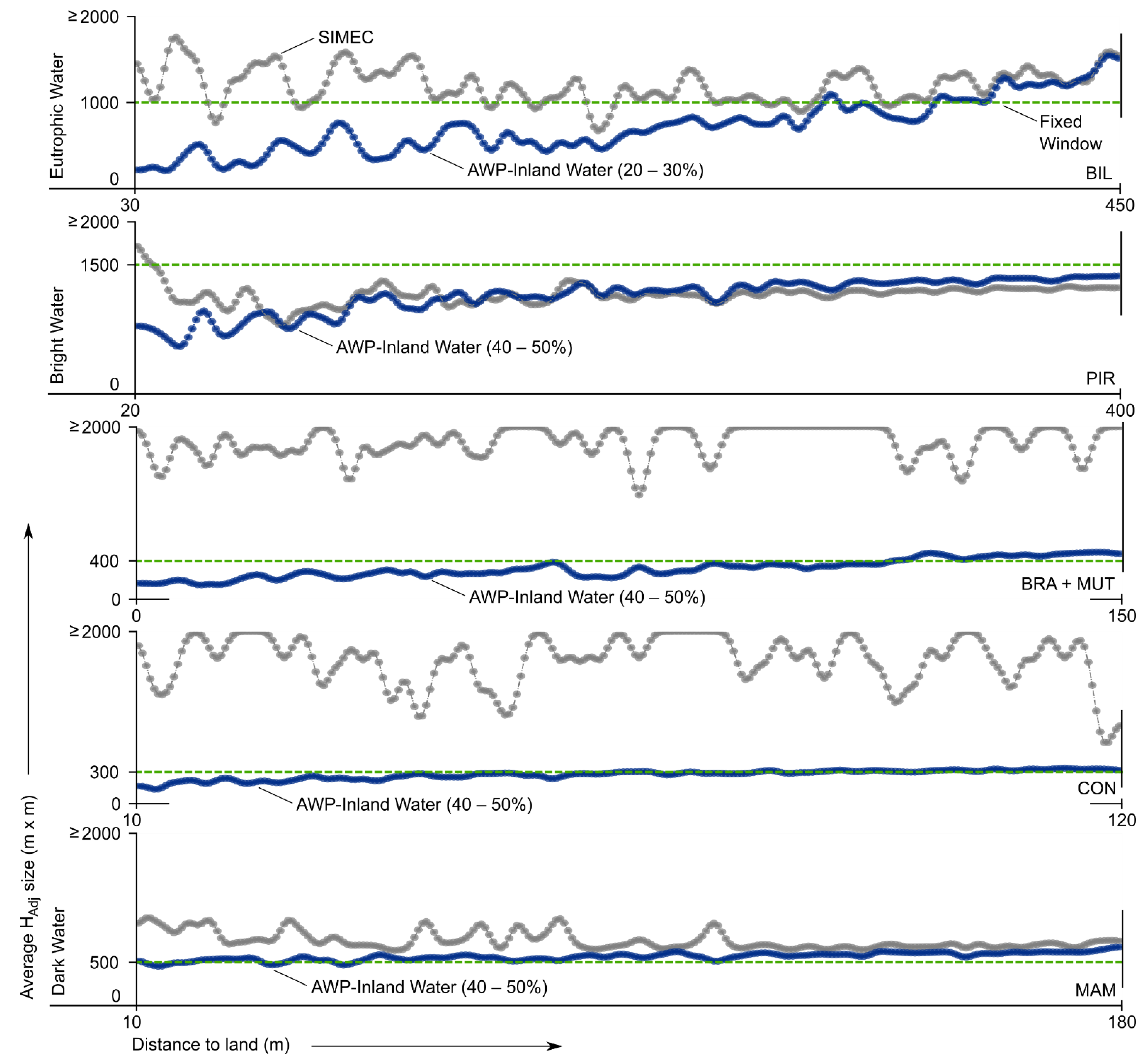
3.2. Range of the Adjacency Effect

The methods applied to retrieve the H Adj generated different results (Figure 4). The adaptive methods, SIMEC and AWP-Inland Water, showed substantial differences located mainly close to the land cover. In general, the differences of H Adj   around the land–water boundary (or waterline) (distance smaller than 100 m) were up to three times higher than that of the regions far from the waterline (distance larger than 100 m). This difference was even more outstanding in the BRA, MUT, and CON lakes. The SIMEC approach, for instance, resulted in an H Adj   several times greater than those estimated by the AWP (average window ~400 m × 400 m) and fixed window (~350 m × 350 m) methods, including infinite H Adj   values (larger than 2000 m × 2000 m). SIMEC did not show any relationship with the distance to the waterline. In contrast, the range of the adjacency effect obtained from the AWP algorithm increased with increasing distance value. This relationship ( H Adj   versus distance to the waterline) was highlighted in the larger (e.g., BIL) and wider (e.g., PIR, BRA, and MUT) water bodies.
Each water body showed an adequate H Adj or proportion of non-water targets within the window for the fixed window and AWP methods, respectively. Despite their empirical nature, the results indicated that the aerosol loading (required for AC) provided information about the proportion of non-water targets needed for the AWP algorithm. Note that, for water bodies under heavy aerosol loadings (larger than 0.3), the desirable proportion of targets was 40–50%, while for lower aerosol loadings (smaller than 0.3), the proportion of non-water targets within the window was 20–30%. Overall, the range of the adjacency effect was higher for lower aerosol loadings. However, PIR presented high H Adj values, despite its high aerosol loading (AOD550 ~0.34). In addition to the aerosol scattering effect, the water type also seemed to influence the size of the H Adj . Comparing the PIR and MAM lakes, which were under similar atmospheric characteristics and aerosol scattering effects (Appendix B, Table A1), different H Adj sizes were obtained, with the dark-water lake demanding a smaller H Adj than the bright-water lake. This is explained by the decreased contrast between the water and the targets around the water body. As bright waters have higher reflectance values, more homogeneous surfaces and, consequently, lower adjacency contributions are expected. Conversely, the atmosphere scattering surpassed the reflectance of the adjacent target under high aerosol loadings, generating more significant adjacency effects. In these cases, larger H Adj were needed to compute the existing adjacency effect values.
The MSI-derived water reflectance associated with the H Adj estimation is displayed in Figure 5 and Figure 6 for four MSI near-infrared bands (705, 740, 783, and 842 nm) and three optical water types. It is evident that the H Adj difference effect produced from the three methods increased with increasing wavelength because the larger wavelengths had a sharp reflectance contrast between the water and various land targets (e.g., soil and forest). The AWP algorithm underestimated, significantly, the reflectance values of dark waters. At the same time, the SIMEC and the fixed window approaches in this water type caused an expressive overcorrection of the water reflectance beyond 740 nm.
In the case of dark waters, both the SIMEC and fixed window approaches showed a frequent negative retrieval of water reflectance (or invalid value) at the near-infrared wavelengths (average frequency ~56% and ~25%, respectively). At 842 nm, SIMEC produced up to twenty times more invalid values than AWP-Inland Water. Similarly, the fixed window method produced about ten times more negative results when compared to AWP. In another way, the eutrophic and bright waters presented a satisfactory agreement between the methods, especially between SIMEC and AWP. In these optical scenarios, the number of invalid results was small (~5%, on average). Again, negative values were high at 842 nm compared to other bands. For that band, the SIMEC and fixed window methods generated more significant inconsistencies in estimating water reflectance for eutrophic (~13%) and bright (~17%) waters, respectively.

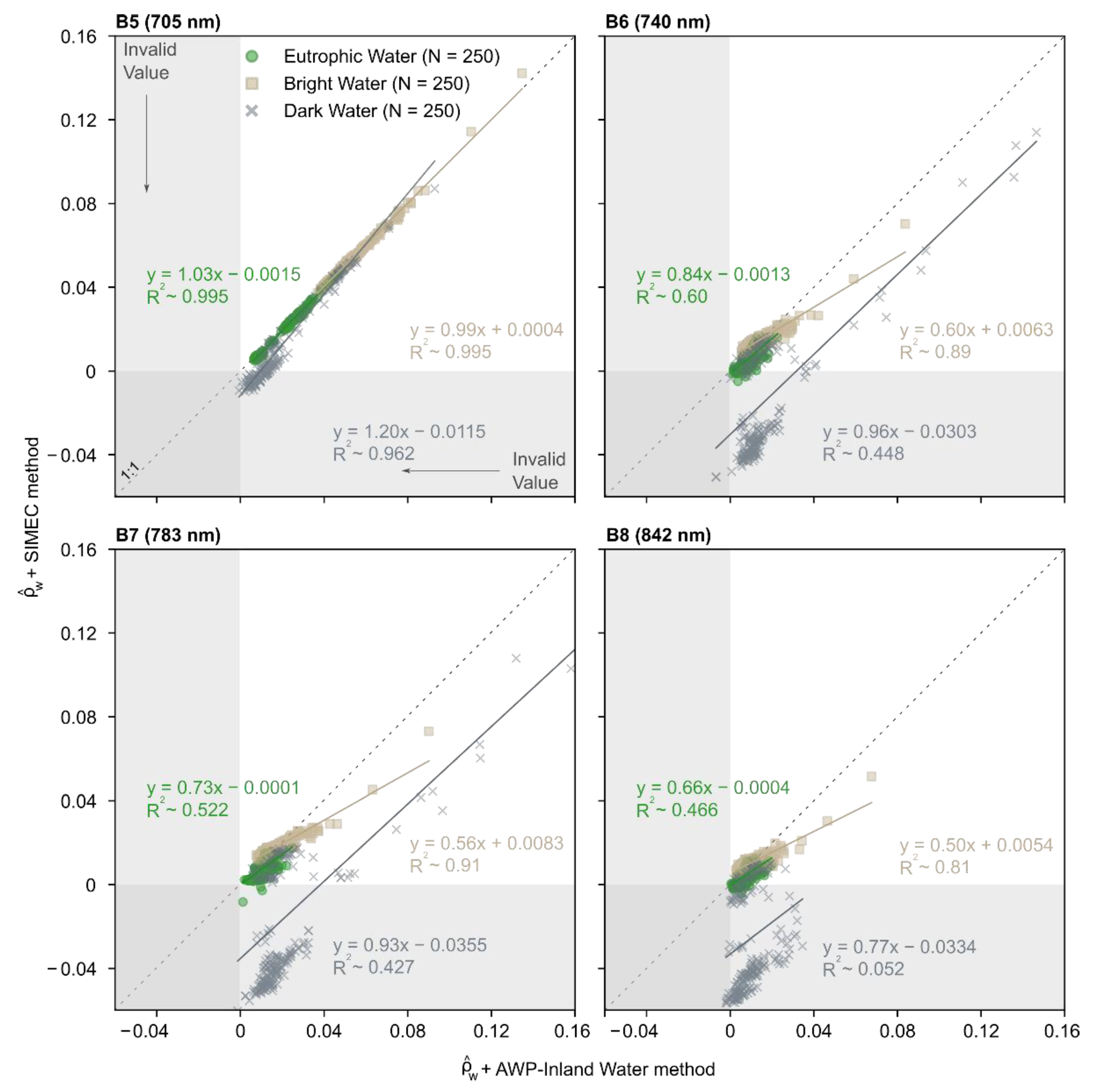
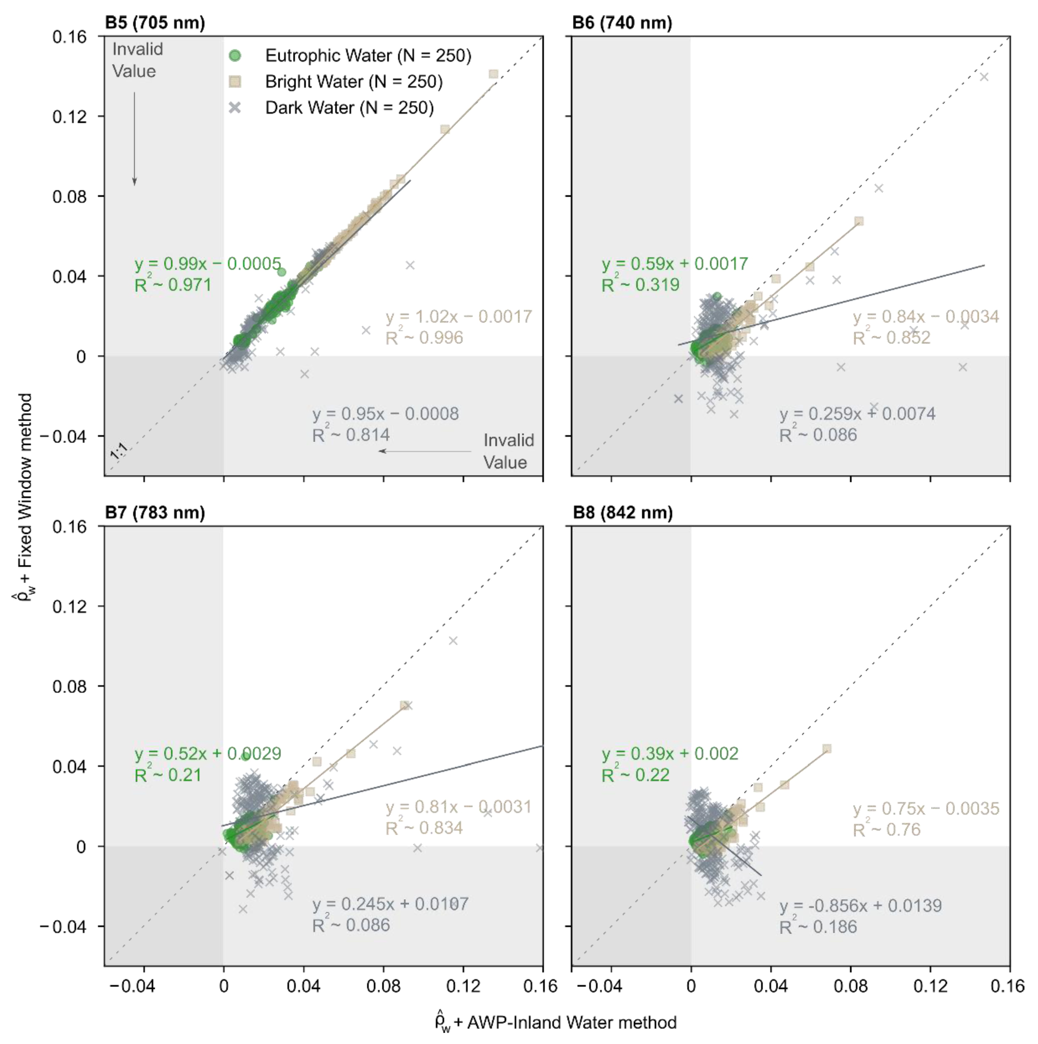
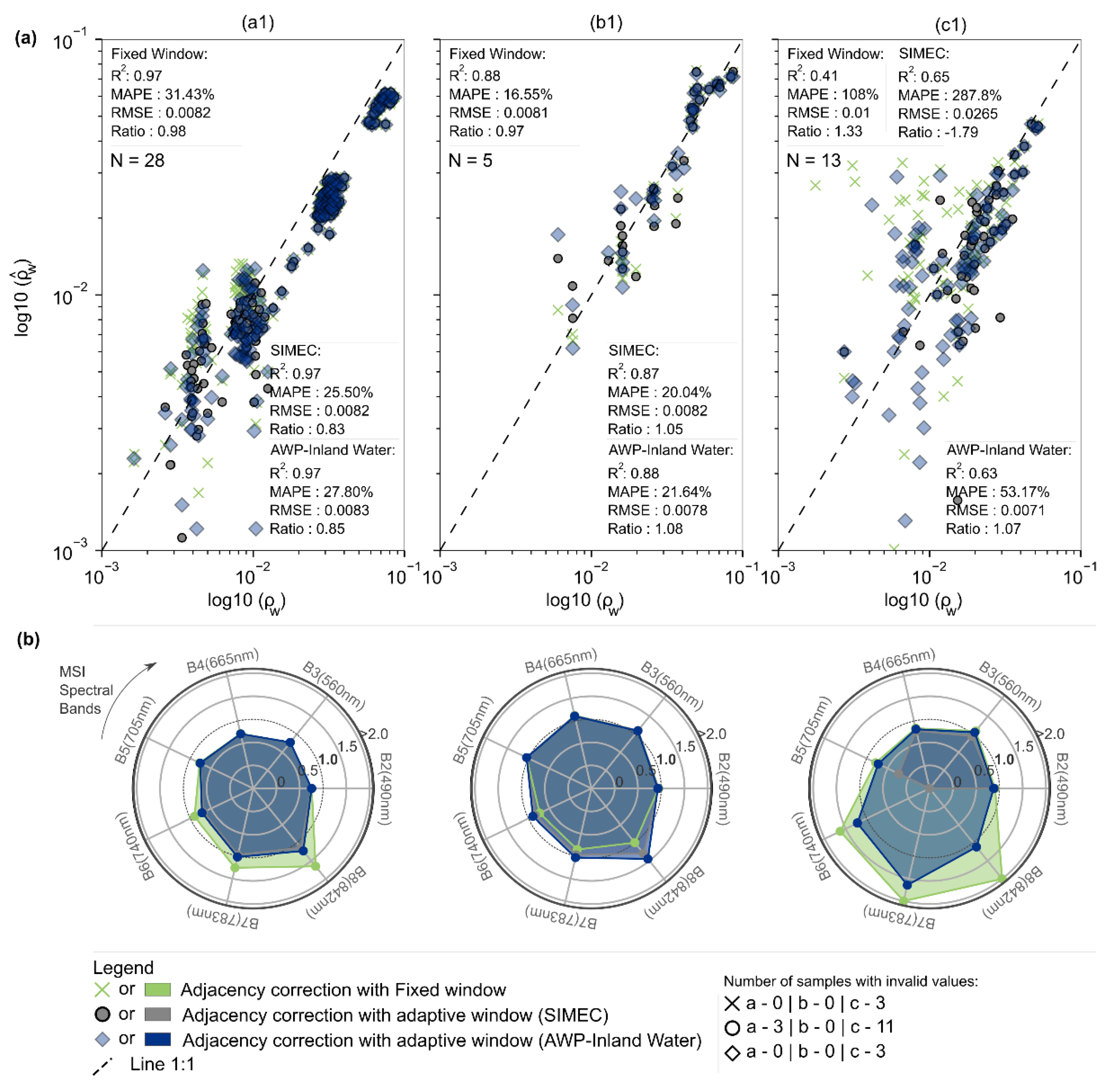
3.3. Adjacency Effect Correction

In general, accurate observations of the satellite-derived water reflectance were obtained after adjacency effect correction for all water types (Figure 7). AWP-Inland Water, as well as SIMEC, demonstrated a good agreement between MSI and in-situ measurements of water reflectance for the eutrophic and bright waters (MAPE smaller than ~28%) (Figure 7a). In these environments, the difference between the performance of these two methods was minimal (~3%). In contrast, only AWP reached a more accurate water reflectance estimate in dark water environments (MAPE ~53%). The number of invalid results (i.e., negative water reflectance values) in the dark waters was remarkably high using SIMEC. In fact, the overcorrection for adjacency effects in the near-infrared wavelengths can leads to negative values due to the low water reflectance. The bright waters showed smaller uncertainties from adjacency effect correction when using the fixed window approach (MAPE ~16.55%). However, as indicated in Section 3.2, this method often produced invalid results for these water types. This fact suggests that the small number of samples used to validate the adjacency effect correction may have limited a representative statistic in bright waters.
In eutrophic and dark waters, the fixed window approach applied to correct the adjacency effects caused underestimation of the reflectance values at 783 nm and 842 nm (average ratio more than ~1.3 and ~1.6, respectively) (Figure 7b). In the case of bright waters, its performance was superior to that of the other methods at 842 nm considering only the dataset available for validation. AWP slightly underestimated the water reflectance at 842 nm when compared to SIMEC in bright and eutrophic waters. The dark waters were more sensitive to the differences in the H Adj size applied to correct the adjacency effects. SIMEC in all near-infrared wavelengths (from 705 nm to 842 nm) had a poor performance for correcting the target effects around these small lakes. On the other hand, recognizing the challenges of estimating the satellite-derived water reflectance of water bodies with very low reflectance under atmospheric complexity, AWP-Inland Water showed acceptable results, despite the poor results at 783 nm.
Figure 8 shows an overall (i.e., average water spectrum plus its standard deviation) water spectrum shape comparison between MSI and in-situ measurements after adjacency effect correction performed using the fixed window, SIMEC, and AWP-Inland Water approaches to estimate the size of the H Adj according to the water types. At first glance, the adjacency effect correction significantly improved the water spectrum shape across all four near-infrared bands of MSI. The adjacency effect mainly was reduced in this spectral domain and was practically nonexistent in the visible wavelengths. At the water surface, the near-infrared wavelengths usually are more impacted by targets neighboring the water body, as previously discussed. However, errors in estimating the range of the adjacency effect can also produce overcorrection in the visible spectral domain. The inaccurate performance of SIMEC in dark waters changed the water spectrum shape at 560 nm and 665 nm. Evidently, the AWP method showed a good agreement with the field spectra of the different water optical compositions. The physical method employed to correct the adjacency effect, associated with a good computation of H Adj , allowed the correct estimation of the water reflectance under high aerosol loadings (in the case of small Amazon lakes) and lower aerosol loadings (in the case of BIL). If the adjacency effect is not corrected, the water reflectance can heavily impact the retrieval of OACs, especially for bio-optical algorithms that use larger wavelengths to infer about the water composition.

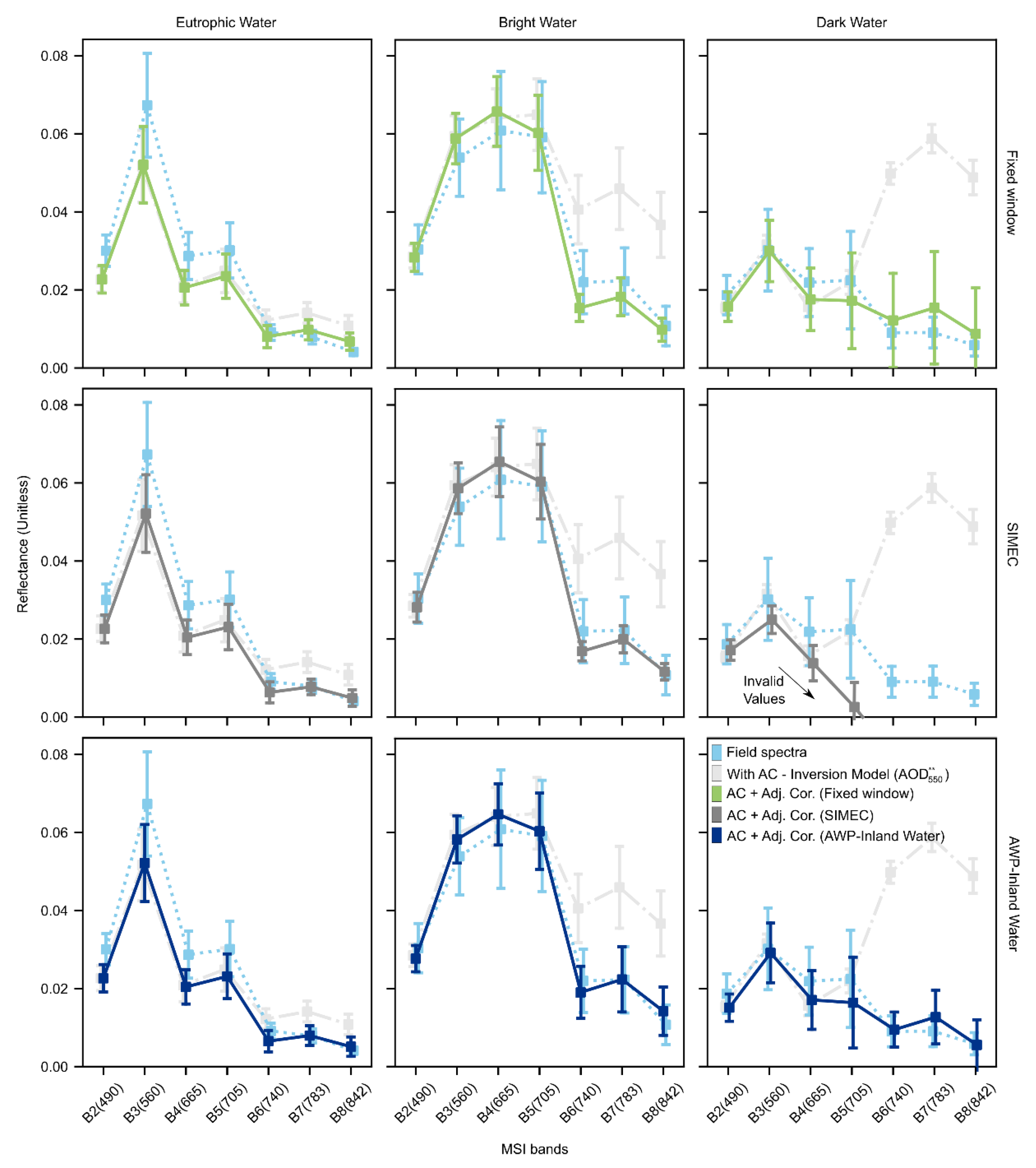
3.4. Adjacency Effect Influence on Water Bodies

The adjacency effect is highly dependent on the atmosphere scattering processes. Notably, its magnitude increased with increasing AOD550 parameters. For imagery acquired under lower aerosol loadings, as in the case of eutrophic waters, the adjacency effect contribution at the top-of-atmosphere was smaller than ~30% throughout the wavelengths (Figure 9). In comparison, in the bright and dark waters observed under high aerosol loadings, this contribution was ~20% at visible wavelengths, reaching up to ~80% in the near-infrared domain. The spectral differences of the adjacency effect depended on the target type surrounding the water body and the optical characteristics of the water itself. For example, at 560 nm, all water bodies presented a peak in adjacency contribution related to the vegetation cover around the water bodies. However, this phenomenon occurred in BIL due to vegetation around it, as well as algae present in the water column. Note that BIL’s TOA contribution was approximately ~60% in this band. In the 740 nm–842 nm range, the adjacency contribution was up to ten times higher than that of the dark waters, justifying why this water type was drastically affected by the adjacency effects in our observations. On the other hand, this difference dropped substantially for other water types (~1.2 times and ~2.3 times more than the eutrophic and bright waters, respectively).
By exploring each water body, the absolute adjacency effect reflectance ( ρ adj ) estimated in BIL (maximum ρ adj ~3%) was often smaller when compared to the PIR and MAM lakes (~6%) or Juruá River floodplain lakes (~12%) when using the MSI band at 842 nm as a reference (Figure 10a). Overall, the ρ adj was more significant for locations close to the edges and narrow areas, and it was smaller at the center of the water bodies. However, in BIL, the maximum ρ adj values occurred in areas with intense algal bloom. These events of algal bloom produced a significant increase of water reflectance at 842 nm, generating large contrast between the regions with and without algal blooms (Figure 10b). Along the A     A transects, an inverse combination between the amount of ρ adj and the difference of corrected and uncorrected reflectance in eutrophic and bright waters was shown. This also occurred due to heterogeneous surfaces generated from the variability in water composition. On the contrary, in the case of dark water lakes, these two factors were directly related, i.e., the reflectance differences increased with the increase of ρ adj .
The correction of the adjacency effect varied spatially in response to these reflectance changes in the H Adj . The transects showed that the smaller the water reflectance values, the more affected the water signal by the adjacency correction due to higher contrast with the neighborhood signal. For example, for waters with algal bloom or sediment dominance, the shorter spectral reflectance difference from the water and land targets can reduce the effect of surrounding targets on the water body. The water bodies experienced a reflectance decrease of up to −170% after the correction of the adjacency effect at 842 nm. The adjacency effect correction was larger in the small Amazon lakes (average value around −80%). For BIL, these results were even smaller (average value approximately −35%). In this system, the Pedra Branca, Rio Grande, and Rio Pequeno arms were more impacted compared to the other BIL’s sections because they are very narrow and are less affected by algal bloom. Interestingly, the adjacency correction induced a slight increase in the water reflectance over the areas with intensive algal bloom (water reflectance difference less than ~6%), which is partially explained by higher target pixel reflectance values than the adjacent pixels.

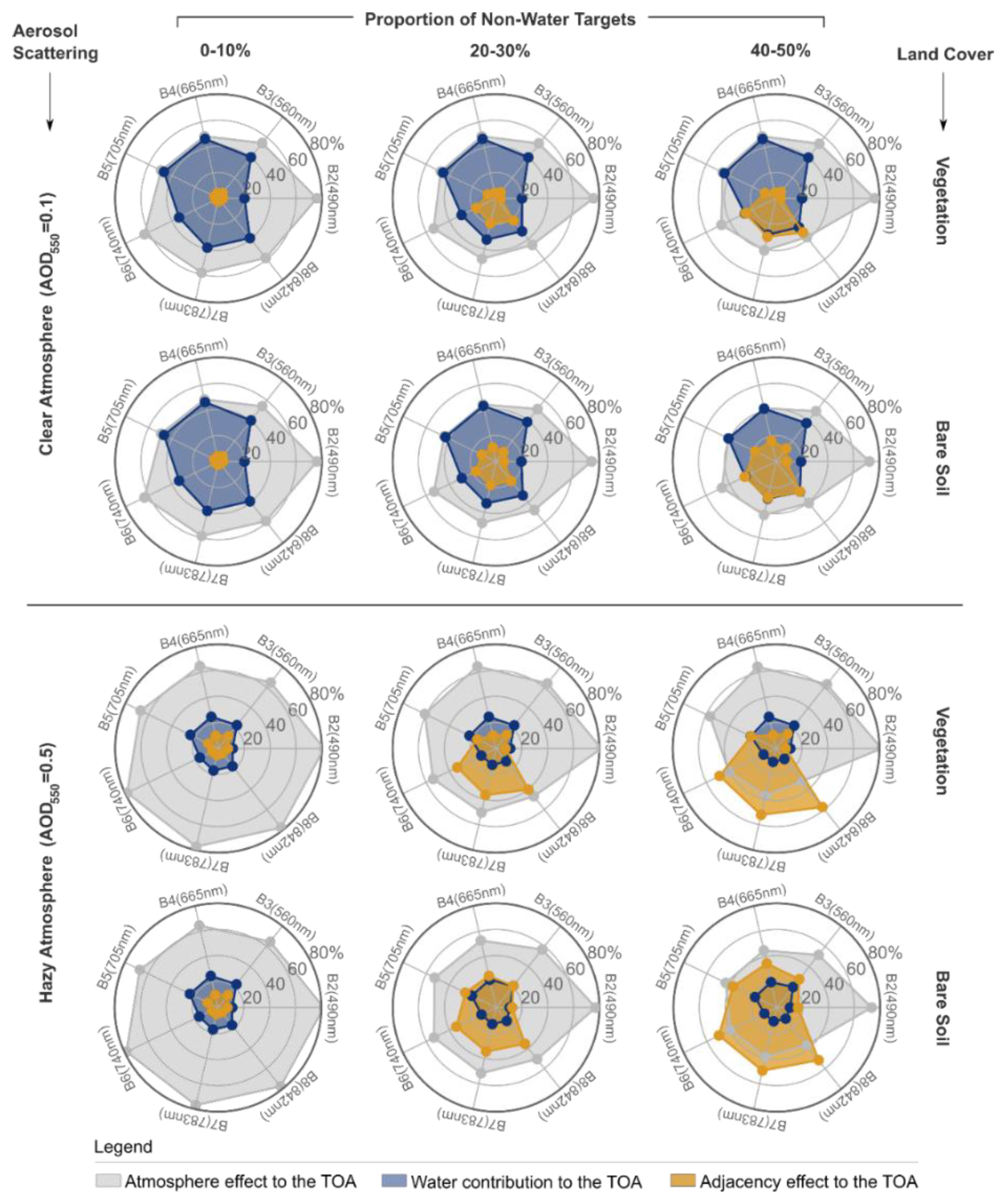
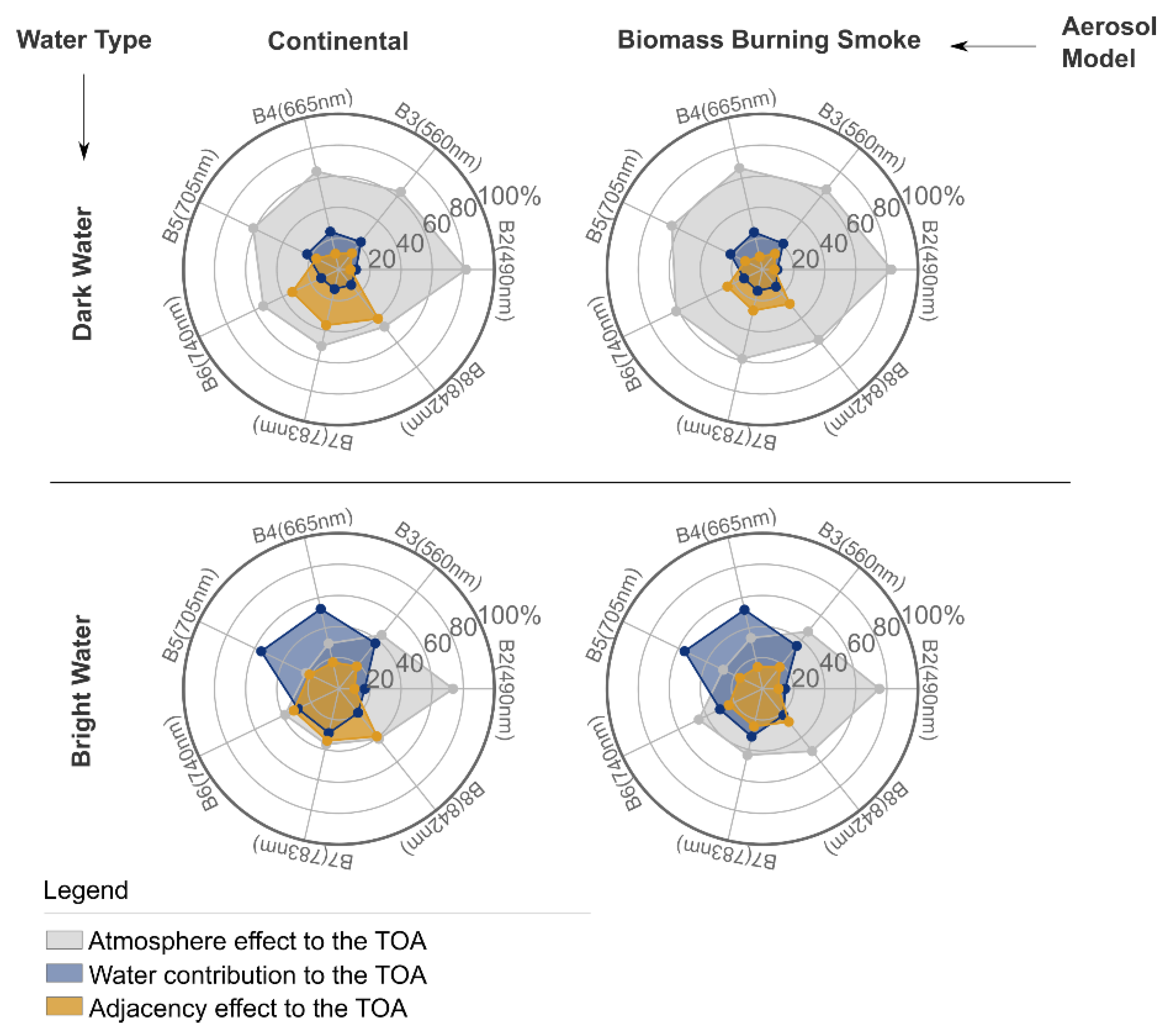
3.5. Sensitivity of Adjacency Effect at the TOA

Here, the sensitivity of the adjacency effect to the proportion of non-water targets within the H Adj , land-cover type around the water body, water optical type, aerosol loading, and aerosol model is investigated. For that, we simulated the adjacency effect contribution at the TOA, assuming fixed atmosphere characteristics to run the 6SV model (Appendix B, Table A2). The sensitivity assessment to the aerosol model was based on the standard models embedded in 6SV (e.g., continental and biomass burning smoke). All runs considered only a water pixel distant 0 m from the waterline. The results in terms of the proportion of non-water targets within the window showed an increase in the adjacency effect magnitude in response to the proportion of non-water targets (Figure 11). For example, at 842 nm, the difference between the adjacency effects of the 40–50% (~33%) and 0–10% (~2%) proportion was ~31%, under a clear atmosphere (AOD550 = 0.1). Already in a condition with heavy aerosol loadings (AOD550 = 0.5), this difference was even greater at ~53%. The water was more affected by the adjacency effect under high aerosol loadings. Note that, for higher AOD550 values, the adjacency effect was several times higher than the water signal at the TOA (up to ~5 times larger for the proportion of 40–50% at 740–842 nm wavelengths). The difference between the adjacency effect and water contribution was tiny (up to ~1.1 times larger) under lower aerosol loadings. The cover type around the water body showed greater differences in the adjacency contributions at 560–705 nm wavelengths due to changes in the spectral response between the bare soil and vegetation targets. Specifically, when varying the land-cover type for bare soil and vegetation, the water body was less impacted by the adjacency effect changes generated from these surrounding targets at larger wavelengths.
The aerosol models caused different adjacency effect contributions at the TOA (Figure 12). In general, the biomass burning smoke aerosol model produced a smaller adjacency effect when compared to the continental model. The average difference between the adjacency effects generated by the two models was about 10% in the 705–842 nm spectral range. This is explained by the increased radiation absorption from the type of aerosol particle inserted in the biomass burning smoke model. The adjacency effects showed a slight sensitivity to water type at the shorter wavelengths. In this case, the adjacency contribution increased with the increasing water reflectance. The difference in the adjacency effects produced from the variation of dark and bright waters was ~3%.

4. Discussion

4.1. Aerosol and Atmospheric Correction

The recovery of aerosol loading over inland waters has a crucial role in accurately correcting the atmospheric scattering effect on satellite images, and errors in its properties affect the water reflectance measurement. The aerosol loadings extracted from MODIS did not perform well for high aerosol loadings (more than 0.3) compared to the AOD 550 * * based on the inversion model (see Figure 3). Some limitations of the MODIS aerosol product are related to sensor characteristics, surface assumptions, and the aerosol model [61,63,64]. In general, the errors observed for a clear atmosphere occur due to the assumptions adopted for the surface, and for a hazy atmosphere, the errors respond to the aerosol model assumptions [61]. Thus, even though the forest areas surrounding the Amazon floodplain lakes are well-correlated with the MODIS aerosol product (R ~0.88) [65], the atmospheric aerosol complexity surpasses the surface influence due to the high aerosol loadings [66]. Furthermore, the type of aerosol model implemented is another uncertainty source in atmospheric correction over inland waters. Therefore, model selection is crucial to represent the aerosol characteristics in the water body region, and when this is incorrect, errors are introduced in satellite-derived water reflectance under high aerosol loadings [28]. All these inconsistencies associated with AOD550 recovery did not stand out in the inversion model, potentially because it estimated the aerosol values in response to the best observation of water reflectance (i.e., field data). Though the initial results are promising, the aerosol loading inversion method requires in-situ water reflectance, and when the method assumptions are not completely fulfilled (e.g., TOA signal free from glint or adjacency contamination), it does not work.
The Amazon region has several aerosol sources, such as biogenic from the rainforest (e.g., fungal spores and volatile organic compounds), black carbon particles from biomass burning, and urban aerosol [67,68,69]. Those sources have distinct characteristics in wet and dry seasons [67,70], altering aerosol properties [71]. Consequently, the variability of aerosol effects (composition + aerosol load) in this region may not be fully represented by the default aerosol models available for use [72], limiting the application of standard procedures for aerosol recovery. For example, Flores Júnior et al. [73] showed a fair amount of error in OLCI blue spectral bands (more than 100% at 400 nm–490 nm) during AC with the MODIS aerosol product, impacting the use of image-derived reflectance for the retrieval of inherent optical properties. In addition to problems related to the aerosol loading recovery for inland waters, the different water reflectance values displayed over the larger wavelengths can introduce further uncertainty into OACs estimation [19,74]. These wavelengths are strongly affected by gas absorption (e.g., water vapor and oxygen at 700 nm–800 nm) [62] and by the photons of energy reflected from surfaces around the water body (so-called adjacency effect) [17,33]. The adjacency effect depends on the atmosphere scattering conditions and, therefore, is well-correlated with the aerosol optical depth [24]. Adjacency effect correction is typically needed in small water bodies and high aerosol loadings [12], limiting, when neglected, the use of remote sensing data at near-infrared wavelengths for water quality application [10]. Although significant efforts have been made to improve the performance of the atmospheric correction algorithms in aquatic ecosystems over time [75], our results indicated that there are still unresolved challenges for inland waters. In complex atmospheric aerosol conditions, careful estimation of aerosol optical depth in these environments using the inversion model is particularly pertinent to achieve the required accuracy of water reflectance for water quality mapping.

4.2. Estimation of the H A d j over Inland Waters

Three strategies to recover the size of the H Adj were assessed in this study. The estimation of H Adj   is essential for a more accurate correction of adjacency effects on inland waters. However, the complex dependence of the range size on multiple factors (e.g., atmosphere scattering, viewing and illumination geometry, spectral characteristics of the surrounding target, and characteristics of satellite sensors) seems to limit a feasible estimative of H Adj for correcting adjacency effects. There is no precise formula available to define the size of the H Adj . Previous studies have shown that the adjacency effect influences in the order of tens of kilometers from the coastline over coastal waters [17,34]. In contrast, values in good agreement with the aerosol scale height in the atmosphere (between 0.5 and 1.0 km) have generally been used for land and water applications [25,27,28]. This study computed an H Adj between 0.1 and 2 km, considering all the methods employed to recover the range of the adjacency effect. The three strategies investigated showed a vast difference concerning the estimation of H Adj . For example, the average difference between SIMEC and AWP-Inland Water in dark-water lakes was ~0.8 km. In contrast, this difference was smaller for the fixed window and AWP methods (average difference ~0.06 km). These results strongly affected the MSI-derived water reflectance, especially at the near-infrared wavelengths. As previously discussed, these wavelengths refer to the spectral domain with the more significant adjacency contribution on inland waters. They are commonly related to an increase in land reflectance and a decrease in water reflectance. The resulting estimates of H Adj demonstrated a linear relationship with the aerosol optical depth at 550 nm, where the size of the H Adj decreased with increasing aerosol loading observed on water bodies. A similar pattern was reported in [27]. The adjacency effect receives a greater contribution from distant targets under relatively small aerosol loading (less than 0.2). On the other hand, if the aerosol loading is high (more than 0.3), the adjacency effect is more affected by the water and its neighbors due to decreasing atmosphere transmittance and the increase in forward scattering (related to aerosol particles) [24]. Differently, for higher aerosol loading (AOD550 of 0.3 to 0.5; see Figure 5 in [76]) combined with a more elevated surface reflectance, the surface reflectance exercises an effect on the size of the H Adj , modifying the relationship between the H Adj and aerosol loading, as we observed in the case of bright water.
Generally, our approach (AWP-Inland Water) had the best performance in determining the water reflectance, particularly in dark water environments (see Figure 7). Over inland waters, especially small lakes and reservoirs, the water body geometry (e.g., shape and size of water body) is often variable. Thus, a dynamic and challenging relationship between the water pixels and their surrounding targets is established. This configuration did not benefit the use of the fixed window method for inland waters, since it tended to over- and under-correct the reflectance of water pixels near and far from the waterline, respectively. The improved correlation between MSI and in-situ measurements of water reflectance shown by AWP-Inland Water indicated that the iterative changes in the window sizes explain the best performance of the method. The AWP-Inland Water method fulfills the essential relationship between window size and distance from the land (see Figure 4) by considering what is inside the window (water or non-water targets) to compose the adjacency effect magnitude. However, the proportion of non-water targets within the window can be variable for each water body in response to the adjacency effect. The relationship between the proportion of targets versus aerosol loading determined in this study can guide its definition in future AWP applications. In comparison to the fixed window and AWP methods, SIMEC demonstrated a good performance in the eutrophic and bright waters but a deficient performance in the dark waters. SIMEC often generated infinite H Adj values (larger than 2 km × 2 km) and, consequently, invalid results (see Figure 5). The dark waters were the most affected by the production of invalid results. As previously discussed in Section 2.5.1., in conditions where the NIR similarity spectrum assumptions are not satisfied, the SIMEC approach may not work [18,33]. Considering that the similarity spectrum was designed for turbid and coastal waters [59], this may prevent its use for inland waters, particularly in dark waters.

4.3. Influence of Adjacency Effect on Water Reflectance Data

The relationship between the magnitude of the adjacency effect versus aerosol scattering is well-discussed [24]. In our case, it is evident that high aerosol loadings favored the occurrence of the adjacency effect. In the eutrophic waters observed under lower aerosol loadings, the water reflectance surpassed the adjacency effect at the top-of-atmosphere for the whole spectral range (see Figure 9). On the other hand, in the small lakes, the adjacency effect was more remarkable. In agreement with these results, a previous study indicated the sensitivity of the small Amazon floodplain lakes to the adjacency effects [12]. These environments maximize adjacency effects due to atmospheric aerosol complexity (Section 4.1), lake size and shape, canopy stand, the vigor of the surrounding forest, and water optical type. Note that the proportional contribution of the effect was more significant for the dark-water lakes than for the bright-water lake. This is explained by the lower reflectance of dark waters due to water absorption and colored dissolved organic matter. The impact of scattered radiation from surrounding targets was significantly larger closer to waterline. However, in conditions of algal blooms or high sediment loadings, the water body pixels close to these events were impacted by adjacency correction due to the contrast between spectral signatures caused by the different concentrations of water optical components (see Figure 10b). The algal blooms and high sediment loadings could significantly increase water reflectance in the near-infrared domain, making the water reflectance similar to that of land targets. This explains why the pixels with higher water reflectance values were less affected by adjacency correction, as depicted in Figure 10b. When the water reflectance is much higher (e.g., in the case of an intense algal bloom in the near-infrared region) than that of its neighboring pixels, the adjacency effect leads to a decrease in the water reflectance value. Note that the adjacency effect is a flux of photons produced by atmospheric scattering directed from bright to dark targets [77]. Then, on no-uniform surfaces, this effect causes a decrease in photons on high-reflectivity surfaces (e.g., bloom areas) as a function of the low-reflectivity surfaces (e.g., areas around the blooms). In this way, adjacency effect correction compensates for the photons lost by the bright targets, i.e., it removes the incremented photons on dark surfaces and returns them to bright surfaces. Hence, small increases may occur in water reflectance when corrected for adjacency effects, giving positive differences between the corrected and uncorrected MSI-image reflectance, as reported here. This behavior is frequently observed in the adjacency correction of surfaces with a high contrast in coverage [27,28,30].

4.4. Sensitivity and Challenges of Adjacency Effect

The adjacency effect magnitude has been little investigated in applications with inland waters. Based on this study, the main factors influencing the increase or decrease of adjacency effects over inland waters were the aerosol loading, aerosol model, land-cover type, and H Adj . Indeed, heavy aerosol loadings and higher atmospheric scattering conditions (as in the continental aerosol model) maximized the adjacency effect, since it originates from the atmospheric scattering [24]. Thus, the results indicated that it may not be necessary to implement adjacency effect correction for cases of very low AOD550 (smaller than 0.1) (see Figure 11). Furthermore, the land-cover type around water bodies also influences the adjacency contributions. As the reflectance of the surrounding targets increases, so did the adjacency effect [17,24]. The effect related to bare soil cover was more significant in the visible domain compared to vegetation cover. However, these two covers produced a minimal difference in the adjacency contributions at larger wavelengths due to their reflectance similarity. Regarding water type (Figure 12), the adjacency effect was less sensitive to the variation of water optical composition (~3% at the visible domain). A previous study has shown that this difference depends on the type of land cover around water bodies [17]. The changes in the adjacency contribution at the TOA caused by water type are more significant when the land targets had low reflectance due to the importance given to water reflectance in modeling the adjacency effect. In addition, other factors that may influence the adjacency effect have been reported in the literature, such as viewing and illumination geometry, satellite spatial resolution, and glint contributions [34,58,78].
The physical approach [15,21] performed well in correcting the adjacency effects over inland waters. However, the strong sensitivity of the method to the size of H Adj , as remarked in our study, may limit an accurate quantification of the adjacency effect in real applications. Additionally, the APSF weights defined from the molecular and aerosol scattering effects (see Equation (9)) also seem to influence the adjacency contribution. Sei [22] showed that the increase of APSF weight produced much larger ranges of adjacency effect because the targets around the water pixel received greater importance compared to lower APSF weights. Comparing the weight approach with a methodology based on three-dimensional radiative transfer simulations applied over coastal waters, Bulgarelli and Zibordi [17] reported an increase of adjacency effects close to land (~70%) from the use of APSF weights to compose the effect magnitude. Even though adjacency effect determination requires highly complex approaches and the physical method has its limitations, our positive experience with this method and the AWP method in estimating H Adj opened a feasible way to correct adjacency effects over inland waters.

5. Conclusions

This paper assessed the feasibility of a physical approach based on APSF to correct the adjacency effect in medium spatial resolution satellite imagery on small lakes surrounded by dense forest cover and a large urban water reservoir considering variable aerosol loadings. This study showed that an iterative inversion model minimized the limitations related to MODIS-derived aerosol loadings and surpassed other sources of uncertainty (e.g., the aerosol model). This careful estimation of aerosol loading is proper in regions of complex atmospheric aerosol conditions (e.g., hazy atmospheric conditions), where the uncertainty of MODIS aerosol estimates is higher, or when there are no aerosol ground-based stations (e.g., AEORONET) around the interest area, as in the case of our study areas.
Adjacency effects impact the reflectance of inland water, and the application of physical methods can remove them from satellite imagery with various degrees of success. In general, none of the empirical approaches used to determine the H Adj presented an outstanding performance for all the selected water types. The three approaches indicated a better recovery of water reflectance in eutrophic and bright waters. Regarding dark waters, only AWP-Inland Water (MAPE ~53%) exhibited improvements, partly because: (i) this water type was outside of the range suggested by SIMEC (~289%) and (ii) the water body geometry changes (e.g., shape and size of water bodies) decreased the performance of the fixed window approach (~108%). In addition, the combination of low water reflectance (e.g., dark waters) and higher adjacency contribution made it challenging to estimate water reflectance accurately. As shown in Figure 9, the adjacency contribution at the TOA exceeded the dark water contribution in such a way that the sensitivity of these waters to the adjacency effect was high. Thus, defining a proper H Adj is crucial for the best adjacency correction from the physical approach and is very challenging due to the factors that can impact it (e.g., land-cover type around the water body and the distance of water pixels from land cover). Even though the AWP-Inland Water method exhibited acceptable results, there are limitations for operational applications, such as defining the optimal proportion of non-water targets, which may vary according to the magnitude of adjacency effect and the increase in running time due to its pixel-by-pixel iteration.
Over inland waters, the adjacency problem was maximized for small water bodies, higher aerosol loadings (more than 0.1), and dark waters (water reflectance smaller than 4%). On the contrary, our results showed that under lower aerosol loadings (smaller than 0.1) the adjacency effects were very small. The adjacency effect contribution at the TOA (see Figure 11), taking into account a critical scenario (i.e., pixels close to land, dark waters, and a high proportion of non-water targets within the window) was very close to water contribution. In this sense, under clear atmospheric conditions associated with larger water bodies is possible neglecting the adjacency effect in medium spatial resolution MSI imagery. Finally, this paper encourages the application and validation of physical methods for the correction of adjacency effects on inland waters, as well as the development and validation of approaches to more adequately determine H Adj size.

Author Contributions

Conceptualization, R.S.P., V.S.M. and E.M.L.M.N.; methodology and application, R.S.P. and V.S.M.; field data validation, R.S.P., F.N.B. and C.C.F.B.; writing—original draft preparation, R.S.P.; writing—review and editing, V.S.M., E.M.L.M.N., C.C.F.B., L.A.S.d.C. and F.N.B. All authors have read and agreed to the published version of the manuscript.

Funding

This research was funded through the 2017–2018 Belmont Forum and BiodivERsA joint call for research proposals under the BiodivScen ERA-Net COFUND program, and by funding from the following organizations: the French National Research Agency (ANR), the São Paulo Research Foundation (FAPESP), the National Science Foundation (NSF), the Research Council of Norway, the German Federal Ministry of Education and Research (BMBF), and the Foundation BNP Paribas through SABERES Project. The field campaigns were sponsored by the MAS-BNDES (project code 1022114003005); the National Council for Scientific and Technological Development (CNPq) (project code 461469/2014-6); the FAPESP projects (2014/23903-9, 2018/12083-1, 2020/14613-8); and the Coordenação de Aperfeiçoamento de Pessoal de Nível Superior—Brasil (CAPES) (Finance Code 001).

Data Availability Statement

In-situ water reflectance data are available from the authors upon reasonable request. MSI Sentinel-2 (A and B) images (Level 1C) are freely available from the Copernicus Open Access Hub website (https://scihub.copernicus.eu/ (accessed on 10 December 2021)).

Acknowledgments

The authors would like to thank the Instrumentation Laboratory for Aquatic Systems (LabISA)/INPE for optical instrument support used for the in-situ measurements. We also thank ESA for the available Sentinel-2 data.

Conflicts of Interest

The authors declare no conflict of interest.

Appendix A

Accurate estimation of the AOD550 is important to model and remove the atmospheric scattering and adjacency contribution from the images. The potential use of the AOD550 recovered from the image-based approach in atmospheric correction has been demonstrated in several studies [7,57,79]. Briefly, this approach explores the difference between the surface reflectance (no aerosol) and the TOA reflectance (aerosol) of a target contained in the image and with known spectral responses at specific wavelengths to estimate the remote sensing aerosol [79]. Applications using the vegetation as reference targets for obtaining the AOD550 have indicated poor performances in the atmospheric correction of aquatic environments, generally overestimating the water reflectance [11,12]. To accommodate these inconsistences, we used MSI reflectance simulated from in-situ data as reference. The idea was to obtain an optimal AOD550 value that allowed the matching of the water signal observed in-situ with that at the top-of-atmosphere based on the inversion of a radiative transfer equation. Three assumptions were needed to apply the method: (i) the in-situ water reflectance in the deep-blue waveband (at 443 nm) is known; (ii) the difference between the water reflectance and the TOA is due to the atmosphere content, i.e., the TOA signal is free from other factors, such as sun and sky glint, bottom, and adjacency effect; and (iii) for overwater, the retrieved AOD550 value is assumed spatially invariant.
In this paper, an optimal AOD550 value was estimated using an iterative process based on a bisection method. Commonly, this method is applied to solve root-finding problems of mathematical equations. A bisection method uses an initial interval, where the equation’s root is contained, that is iteratively divided into subintervals equally spaced in such a way that there is a better approximation for the value of interest [80]. The iterative process used for the AOD550 retrieval can be written as:
f ( A O D 550 ( k ) , B i ) = | ρ ^ w * * ( A O D 550 ( k ) , B i ) ρ w * ( B i ) |
where the function f expresses the difference between the corrected reflectance of atmospheric effect ( ρ ^ w * * ) (Equation (7)) and in-situ observed reflectance ρ w * (Equation (2)) for a given AOD 550 ( k ) value and spectral band B i . k refers to the iteration number. In the zero-order approximation ( k = 0 ), the AOD 550 ( 0 ) value was calculated using the midpoint of the range [ AOD 550 ( min ) , AOD 550 ( max ) ]. This range included the optimal AOD550 value, and its limits were defined at 0 and 2:
  AOD 550 ( k ) = AOD 550 ( min ) ( k ) + AOD 550 ( max ) ( k ) 2
In the first iteration, the interval initial was divided into two halves, such as [ AOD 550 ( min ) ,   AOD 550 ( 0 )   ] and [ AOD 550 ( 0 ) ,   AOD 550 ( max ) ]. To know which half of the interval in which the optimal AOD550 value is contained, a simple observation of function sign f at the midpoint is performed. If f ( AOD 550 ( min ) )   ·   f ( AOD 550 ( 0 ) ) <   0 , the optimal AOD550 value is contained in the range of [ AOD 550 ( min ) ,   AOD 550 ( 0 )   ]. On the contrary, if f ( AOD 550 ( 0 ) ) ·   f ( AOD 550 ( max ) ) <   0 , it is inserted in the range of [ AOD 550 ( 0 ) ,   AOD 550 ( max ) ]. This process was repeated up to the k-order approximation. The convergence condition of the iterative process is f ( AOD 550 ( k ) ,   B i )   0 . 0001 . These iterative steps contain only simple mathematical operations. Therefore, the estimative of an optimal AOD550 value for atmospheric correction of the images is not very time-consuming. The total time spent to recover the AOD550 parameters using a single field sample and a spectral band was around 600 s. Some strategies can be adopted to reduce the total computation time, such as parallel operations, reducing the size of the initial interval, and increasing the tolerance value of the convergence condition.
All in-situ samples were used in the inversion model of AOD550, except for BIL, where only the samples collected far from the reservoir border were applied. In each water body, the optimal AOD550 value was recovered using the MSI deep blue waveband and the average of the aerosol loading values observed for each in-situ sample. The estimative of the optimal AOD550 value over water bodies was derived from the following equation:
  AOD 550 * * ( w , B db ) = 1 N j = 1 N AOD 550 j ( w ,   B db )
where AOD 550 * * is the average value of the aerosol optical depth for a given water body w , AOD 550 j is the aerosol recovered for a single in-situ sample, B db is the MSI deep blue waveband, and N is the total number of in-situ samples. Note that we did not have in-situ measurements of aerosol optical depth data next to the water bodies. Therefore, it was not possible to validate the optimal AOD550 value obtained by the inversion method directly. Thus, its validation was performed indirectly through the AC.

Appendix B

Table A1. Overview of input data required for the AC for water bodies included in this study.
Input DataBILCONBRA + MUTMAMPIR
Solar Zenith Angle48.22°29.52°29.52°27.78°27.78°
Solar Azimuth Angle33.37°53.65°53.65°61.70°61.70°
View Zenith Angle3.74°2.83°2.83°9.44°9.44°
View Azimuth Angle111.67°194.68°194.68°101.95°101.95°
Ozone (cm-atm)0.2820.2620.2620.2710.271
Water Vapor (g/cm3)1.4823.4183.5624.4074.247
Altitude (km)0.7160.0710.0720.0430.041
Aerosol ModelContinental
AOD at 550 nm *0.1000.3310.2720.1640.170
AOD at 550 nm **0.1620.6560.6330.3690.342
* AOD550 recovered with the MODIS products (MCD19A2 Collection 6). ** AOD550 recovered with the inversion model using the deep blue waveband.
Table A2. Atmospheric parameters and geometric conditions (viewing and illumination) used in the theoretical simulations.
Solar
Zenith
Angle
View
Zenith
Angle
Solar
Azimuth
Angle
View
Azimuth
Angle
Target
Altitude
Aerosol
Model
Atmospheric
Profile
Band Range
33°53°141°0.189
(km)
*Tropical
(default)
443–842 (nm)
* Continental or biomass burning smoke model.

References

  1. Vörösmarty, C.J.; McIntyre, P.B.; Gessner, M.O.; Dudgeon, D.; Prusevich, A.; Green, P.; Glidden, S.; Bunn, S.E.; Sullivan, C.A.; Reidy Liermann, C.; et al. Global threats to human water security and river biodiversity. Nature 2010, 467, 555–562. [Google Scholar] [CrossRef] [PubMed]
  2. Boretti, A.; Rosa, L. Reassessing the projections of the World Water Development Report. Nature 2019, 15, 15. [Google Scholar] [CrossRef]
  3. UNESCO, UN-Water. United Nations World Development Report 2020: Water and Climate Change. Paris: UNESCO. 2020. Available online: https://www.unwater.org/publications/world-water-development-report-2020/ (accessed on 20 January 2022).
  4. Pahlevan, N.; John, R.S.; Franz, B.A.; Zibordi, G.; Markham, B.; Bailey, S.; Schaaf, C.B.; Ondrusek, M.; Greb, S.; Strait, C.M. Landsat 8 remote sensing reflectance (Rrs) products: Evaluations, intercomparisons, and enhancements. Remote Sens. Environ. 2017, 190, 289–301. [Google Scholar] [CrossRef]
  5. Pahlevan, N.; Sarkar, S.; Franz, B.A.; Balasubramanian, S.V.; He, J. Sentinel-2 MultiSpectral Instrument (MSI) data processing for aquatic science applications: Demonstrations and validations. Remote Sens. Environ. 2017, 201, 47–56. [Google Scholar] [CrossRef]
  6. Vanhellemont, Q.; Ruddick, K. Advantages of high quality SWIR bands for ocean colour processing: Examples from Landsat-8. Remote Sens. Environ. 2015, 161, 89–106. [Google Scholar] [CrossRef] [Green Version]
  7. Vermote, E.; Justice, C.; Claverie, M.; Franch, B. Preliminary analysis of the performance of the Landsat 8/OLI land surface reflectance product. Remote Sens. Environ. 2016, 185, 46–56. [Google Scholar] [CrossRef]
  8. Cairo, C.; Barbosa, C.; Lobo, F.; Novo, E.; Carlos, F.; Maciel, D.; Flores Júnior, R.; Silva, E.; Curtarelli, V. Hybrid chlorophyll-a algorithm for assessing trophic states of a tropical brazilian reservoir based on MSI/Sentinel-2 data. Remote Sens. 2020, 12, 40. [Google Scholar] [CrossRef] [Green Version]
  9. Kutser, T.; Paavel, B.; Verpoorter, C.; Ligi, M.; Soomets, T.; Toming, K.; Casal, G. Sensing of Black Lakes and Using 810 nm Reflectance Peak for Retrieving Water Quality Parameters of Optically Complex Waters. Remote Sens. 2016, 8, 497. [Google Scholar] [CrossRef]
  10. Maciel, D.A.; Barbosa, C.C.F.; Novo, E.M.L.M.; Flores Júnior, R.; Begliomini, F.N. Water Clarity in Brazilian Water Assessed Using Sentinel-2 and Machine Learning Methods. ISPRS J. Photogramm. Remote Sens. 2021, 182, 134–152. [Google Scholar] [CrossRef]
  11. Toming, K.; Kutser, T.; Laas, A.; Sepp, M.; Paavel, B.; Nõges, T. First experiences in mapping lake water quality parameters with sentinel-2 MSI imagery. Remote Sens. 2016, 8, 640. [Google Scholar] [CrossRef] [Green Version]
  12. Martins, V.S.; Barbosa, C.C.F.; de Carvalho, L.A.S.; Jorge, D.S.F.; Lobo, F.L.; Novo, E.M.L.M. Assessment of atmospheric correction methods for sentinel-2 MSI images applied to Amazon floodplain lakes. Remote Sens. 2017, 9, 322. [Google Scholar] [CrossRef] [Green Version]
  13. Otterman, J.; Fraser, R.S. Adjacency effects on imaging by surface reflection and atmospheric scattering: Cross radiance to Zenith. Appl. Opt. 1979, 197, 2852–2860. [Google Scholar] [CrossRef] [PubMed]
  14. Richter, R.; Bachmann, M.; Dorigo, W.; Müller, A. Influence of the Adjacency Effect on Ground Reflectance Measurements. IEEE Geosci. Remote Sens. Lett. 2006, 3, 565–569. [Google Scholar] [CrossRef]
  15. Tanré, D.; Herman, M.; Deschamps, Y. Influence of the background contribution upon space measurements of ground reflectance. Appl. Opt. 1981, 20, 3676–3683. [Google Scholar] [CrossRef]
  16. Bulgarelli, B.; Kiselev, V.; Zibordi, G. Simulation and analysis of adjacency effects in coastal waters: A case study. Appl. Opt. 2014, 53, 1523–1545. [Google Scholar] [CrossRef] [PubMed]
  17. Bulgarelli, B.; Zibordi, G. On the detectability of adjacency effects in ocean color remote sensing of mid- latitude coastal environments by SeaWiFS, MODIS-A, MERIS, OLCI, OLI and MSI. Remote Sens. Environ. 2018, 209, 423–438. [Google Scholar] [CrossRef]
  18. Sterckx, S.; Knaeps, E.; Ruddick, K. Detection and correction of adjacency effects in hyperspectral airborne data of coastal and inland waters: The use of the near infrared similarity spectrum. Int. J. Remote Sens. 2011, 32, 6479–6505. [Google Scholar] [CrossRef]
  19. Warren, M.A.; Simis, S.G.H.; Selmes, N. Complementary water quality observations from high and medium resolution Sentinel sensors by aligning chlorophyll-a and turbidity algorithms. Remote Sens. Environ. 2021, 265, 112651. [Google Scholar] [CrossRef]
  20. Sander, L.C.; Schott, J.R.; Raqueño, R. A VNIR/SWIR atmospheric correction algorithm for hyperspectral imagery with adjacency effect. Remote Sens. Environ. 2001, 71, 252–263. [Google Scholar] [CrossRef]
  21. Vermote, E.F.; Tanré, D.; Deuzé, J.L.; Herman, M.; Morcrette, J.J. Second Simulation of the Satellite Signal in the Solar Spectrum, 6S: An Overview. IEEE Trans. Geosci. Remote Sens. 1997, 35, 675–686. [Google Scholar] [CrossRef] [Green Version]
  22. Sei, A. Analysis of adjacency effects for two Lambertian half-spaces. Int. J. Rem. Sens. 2007, 28, 1873–1890. [Google Scholar] [CrossRef]
  23. Vermote, E.F.; Tanré, D.; Deuzé, J.L.; Herman, M.; Morcrette, J.J. Second Simulation of the Satellite Signal in the Solar Spectrum (6S); 6S User Guide Version 3.0.; NASA-GSFC: Greenbelt, MD, USA, 2006.
  24. Minomura, M.; Kuze, H.; Takeuchi, N. Adjacency effect in the atmospheric correction of satellite remote sensing data: Evaluation of the influence of aerosol extinction profiles. Opt. Rev. 2001, 8, 133–141. [Google Scholar] [CrossRef]
  25. Martins, V.S.; Kaleita, A.; Barbosa, C.C.F.; Fassoni-Andrade, A.C.; Lobo, F.L.; Novo, E.M.L.M. Remote sensing of large reservoir in the drought years: Implications on surface water change and turbidity variability of Sobradinho reservoir (Northeast Brazil). Remote Sens. Appl. Soc. Environ. 2018, 13, 275–288. [Google Scholar] [CrossRef]
  26. Wang, T.; Du, L.; Yi, W.; Hong, J.; Zhang, L.; Zheng, J.; Li, C.; Ma, X.; Zhang, D.; Fang, W.; et al. An adaptive atmospheric correction algorithm for the effective adjacency effect correction of submeter-scale spatial resolution optical satellite images: Application to a WorldView-3 panchromatic image. Remote Sens. Environ. 2021, 259, 112412. [Google Scholar] [CrossRef]
  27. Houborg, R.; McCabe, M.F. Adapting a regularized canopy reflectance model (REGFLEC) for the retrieval challenges of dryland agricultural systems. Remote Sens. Environ. 2016, 186, 105–120. [Google Scholar] [CrossRef] [Green Version]
  28. Houborg, R.; McCabe, M.F. Impacts of dust aerosol and adjacency effects on the accuracy of Landsat 8 and RapidEye surface reflectance. Remote Sens. Environ. 2017, 194, 127–145. [Google Scholar] [CrossRef]
  29. Keukelaere, L.; Sterckx, S.; Adriaensen, S.; Knaep, E.; Reusen, I.; Giardino, C.; Bresciani, M.; Hunter, P.; Neil, C.; Van der Zande, D.; et al. Atmospheric correction of Landsat-8/OLI and Sentinel-2/MSI data using iCOR algorithm: Validation for coastal and inland waters. Eur. J. Remote Sens. 2018, 51, 525–542. [Google Scholar] [CrossRef] [Green Version]
  30. Kiselev, V.; Bulgarelli, B.; Heege, T. Sensor independent adjacency correction algorithm for coastal and inland water systems. Remote Sens. Environ. 2015, 157, 85–95. [Google Scholar] [CrossRef]
  31. Pahlevan, N.; Mangin, A.; Balasubramanian, S.V.; Smith, B.; Alikas, K.; Arai, K.; Barbosa, C.; Bélanger, S.; Binding, C.; Bresciani, M.; et al. ACIX-Aqua: A global assessment of atmospheric correction methods for Landsat-8 and Sentinel-2 over lakes, rivers, and coastal waters. Remote Sens. Environ. 2021, 258, 112366. [Google Scholar] [CrossRef]
  32. Pereira-Sandoval, M.; Ruescas, A.; Urrego, P.; Ruiz-Verdú, A.; Delegido, J.; Tenjo, C.; Soria-Perpinyà, X.; Vicente, E.; Soria, J.; Moreno, J. Evaluation of Atmospheric Correction Algorithms over Spanish Inland Waters for Sentinel-2 Multi Spectral Imagery Data. Remote Sens. 2019, 11, 1469. [Google Scholar] [CrossRef] [Green Version]
  33. Sterckx, S.; Knaeps, E.; Kratzer, S.; Ruddick, K. SIMilarity Environment Correction (SIMEC) applied to MERIS data over inland and coastal waters. Remote Sens. Environ. 2015, 157, 96–110. [Google Scholar] [CrossRef]
  34. Bulgarelli, B.; Zibordi, G. Adjacency radiance around a small island: Implications for system vicarious calibrations. Appl. Opt. 2020, 59, 63–69. [Google Scholar] [CrossRef] [PubMed]
  35. Ribeiro, M.S.F.; Tucci, A.; Matarazzo, M.P.; Viana-Niero, C.; Nordi, C.S.D. Detection of Cyanotoxin-Producing Genes in a Eutrophic Reservoir (Billings Reservoir, São Paulo, Brazil). Water 2020, 12, 903. [Google Scholar] [CrossRef] [Green Version]
  36. Wengrat, S.; Bicudo, D.C. Spatial evaluation of water quality in an urban reservoir (Billings Complex, southeastern Brazil). Acta Limnol. Bras. 2011, 23, 200–216. [Google Scholar] [CrossRef] [Green Version]
  37. Alcantara, E.; Coimbra, K.; Ogashawara, I.; Rodrigues, T.; Mantovani, J.; Rotta, H.R.; Park, E.; Cunha, D.G.F. A satellite-based investigation into the algae bloom variability in large water supply urban reservoirs during COVID-19 lockdown. Remote Sens. Appl. Soc. Environ. 2021, 23, 100555. [Google Scholar] [CrossRef]
  38. Leme, E.; Silva, E.P.; Rodrigues, P.S.; Silva, I.R.; Martins, M.F.M.; Bondan, E.F.; Bernardi, M.M.; Kirsten, T.B. Billings reservoir water used for human consumption presents microbiological contaminants and induces both behavior impairments and astrogliosis in zebrafish. Ecotoxicol. Environ. Saf. 2018, 151, 364–373. [Google Scholar] [CrossRef]
  39. Lobo, F.L.; Nagel, G.W.; Maciel, D.A.; de Carvalho, L.A.S.; Martins, V.S.; Barbosa, C.C.F.; Novo, E.M.L.M. AlgaeMAp: Algae Bloom Monitoring Application for Inland Waters in Latin America. Remote Sens. 2021, 13, 2874. [Google Scholar] [CrossRef]
  40. Affonso, A.G.; Queiroz, H.L.; Novo, E.M.L.M. Abiotic variability among different aquatic systems of the central Amazon floodplain during drought and flood events. Braz. J. Biol. 2015, 75, 60–69. [Google Scholar] [CrossRef]
  41. Silva, M.P.; de Carvalho, L.A.S.; Novo, E.; Jorge, D.S.F.; Barbosa, C.C.F. Use of optical absorption indices to assess seasonal variability of dissolved organic matter in Amazon floodplain lakes. Biogeosciences 2020, 17, 5355–5364. [Google Scholar] [CrossRef]
  42. Jorge, D.S.F.; Barbosa, C.C.F.; de Carvalho, L.A.S.; Affonso, A.G.; Lobo, F.L.; Novo, E.M.L.M. SNR (signal-to-noise ratio) impact on water constituent retrieval from simulated images of optically complex Amazon lakes. Remote Sens. 2017, 9, 644. [Google Scholar] [CrossRef] [Green Version]
  43. Maciel, D.A.; Barbosa, C.C.F.; Novo, E.M.L.M.; Cherukuru, N.; Martins, V.S.; Flores Júnior, R.; Jorge, D.S.; de Carvalho, L.A.S.; Carlos, F.M. Mapping of diffuse attenuation coefficient in optically complex waters of amazon floodplain lakes. ISPRS J. Photogramm. Remote Sens. 2020, 170, 72–87. [Google Scholar] [CrossRef]
  44. ESA, European Space Agency. Mission Search. Available online: https://directory.eoportal.org (accessed on 10 December 2021).
  45. Ciancia, E.; Campanelli, A.; Lacava, T.; Palombo, A.; Pascucci, S.; Pergola, N.; Pignatti, S.; Satriano, V.; Tramutoli, V. Modeling and Multi-Temporal Characterization of Total Suspended Matter by the Combined Use of Sentinel 2-MSI and Landsat 8-OLI Data: The Pertusillo Lake Case Study (Italy). Remote Sens. 2020, 12, 2147. [Google Scholar] [CrossRef]
  46. Hestir, E.L.; Brando, V.E.; Bresciani, M.; Giardino, C.; Matta, E.; Villa, P.; Dekker, A.G. Measuring freshwater aquatic ecosystems: The need for a hyperspectral global mapping satellite mission. Remote Sens. Environ. 2015, 167, 181–195. [Google Scholar] [CrossRef] [Green Version]
  47. ESA, European Space Agency. User Guides. Available online: https://sentinel.esa.int/web/sentinel/user-guides/sentinel-2-msi/product-types/level-1c (accessed on 10 December 2021).
  48. Barbosa, C.C.F.; Novo, E.M.L.M.; Martinez, J.M. Remote sensing of the water properties of the Amazon floodplain lakes: The time delay effects between in-situ and satellite data acquisition on model accuracy. In Proceedings of the International Symposium on Remote Sensing of Environment: Sustaining the Millennium Development Goals, Stresa, Italy, 4–9 May 2009. [Google Scholar]
  49. Marinho, R.R.; Harmel, T.; Martinez, J.; Filizola Junior, N.P. Spatiotemporal Dynamics of Suspended Sediments in the Negro River, Amazon Basin, from In Situ and Sentinel-2 Remote Sensing Data. ISPRS Int. J. Geo-Inf. 2021, 10, 86. [Google Scholar] [CrossRef]
  50. Warren, M.A.; Simis, S.G.H.; Martinez-Vicente, V.; Poser, K.; Bresciani, M.; Alikas, K.; Spyrakos, E.; Giardino, C.; Ansper, A. Assessment of atmospheric correction algorithms for the Sentinel-2A MultiSpectral Imager over coastal and inland waters. Remote Sens. Environ. 2019, 225, 267–289. [Google Scholar] [CrossRef]
  51. Capobianco, J.P.R.; Whately, M. Billings 2000: Ameaças e Perspectivas Para o Maior Reservatório de Água da Região Metropolitana de São Paulo. Relatório do Diagnóstico Socioambiental Participativo da Bacia Hidrográfica da Billings no Período 1989–99; Instituto Socioambiental: São Paulo, Brazil, 2002. [Google Scholar]
  52. Affonso, A.G.; Queiroz, H.L.; Novo, E.M.L.M. Limnological characterization of floodplain lakes in Mamirauá Sustainable Development Reserve, Central Amazon (Amazonas State, Brazil). Acta Limnol. Bras. 2011, 23, 95–108. [Google Scholar] [CrossRef]
  53. Barbosa, C.C.F. Sensoriamento Remoto da Dinâmica da Circulação da Água do Sistema Planície de Curuai/Rio Amazonas. Ph.D. Thesis, National Institute for Space Research (INPE), São José dos Campos, Brazil, 2005. [Google Scholar]
  54. Nagel, G.W.; Novo, E.M.L.M.; Martins, V.S.; Campos-Silva, J.V.; Barbosa, C.C.F.; Bonnet, M.P. Impacts of meander migration on the Amazon riverine communities using Landsat time series and cloud computing. Sci. Total Environ. 2022, 806, 150449. [Google Scholar] [CrossRef]
  55. Mobley, C.D. Estimation of the Remote-Sensing Reflectance from Above-Surface Measurements. Appl. Opt. 1999, 38, 7442–7455. [Google Scholar] [CrossRef]
  56. Mobley, C.D. Polarized reflectance and transmittance properties of windblown sea surfaces. Appl. Opt. 2015, 54, 4828–4849. [Google Scholar] [CrossRef]
  57. Lobo, F.L.; Costa, M.P.F.; Novo, E.M.L.M. Time-series analysis of Landsat- MSS/TM/OLI images over Amazonian waters impacted by gold mining activities. Remote Sens. Environ. 2014, 157, 170–184. [Google Scholar] [CrossRef]
  58. Santer, R.; Schmechtig, C. Adjacency effects on water surfaces: Primary scattering approximation and sensitivity study. Appl. Opt. 2000, 39, 361–375. [Google Scholar] [CrossRef] [PubMed]
  59. Ruddick, K.G.; Cauwer, V.; Park, Y.J.; Moore, G. Seaborne measurements of near infrared water- leaving reflectance: The similarity spectrum for turbid waters. Limnol. Oceanogr. 2006, 51, 1167–1179. [Google Scholar] [CrossRef] [Green Version]
  60. Xu, H. Modification of normalised difference water index (NDWI) to enhance open water features in remotely sensed imagery. Int. J. Remote Sens. 2006, 27, 3025–3033. [Google Scholar] [CrossRef]
  61. Levy, R.C.; Remer, L.A.; Kleidman, R.G.; Mattoo, S.; Ichoku, C.; Kahn, R.; Eck, T.F. Global evaluation of the Collection 5 MODIS dark-target aerosol products over land. Atmos. Chem. Phys. 2010, 10, 10399–10420. [Google Scholar] [CrossRef] [Green Version]
  62. Vermote, E.; El Saleous, N.; Justice, C.O.; Kaufman, Y.J.; Privette, J.L.; Remer, L.; Roger, C.; Tanré, D. Atmospheric correction of visible to middle-infrared EOS-MODIS data over land surfaces: Background, operational algorithm and validation. J. Geophys. Res. Atmos. 1997, 102, 17131–17141. [Google Scholar] [CrossRef] [Green Version]
  63. Levy, R.C.; Mattoo, S.; Munchak, L.A.; Remer, L.A.; Sayer, A.M.; Patadia, F.; Hsu, N.C. The Collection 6 MODIS aerosol products over land and ocean. Atmos. Meas. Tech. 2013, 6, 2989–3034. [Google Scholar] [CrossRef] [Green Version]
  64. Lyapustin, A.; Wang, Y.; Korkin, S.; Huang, D. MODIS Collection 6 MAIAC algorithm. Atmos. Meas. Tech. 2018, 11, 5741–5765. [Google Scholar] [CrossRef] [Green Version]
  65. Martins, V.S.; Lyapustin, A.; de Carvalho, L.A.S.; Barbosa, C.C.F.; Novo, E.M.L.M. Validation of high-resolution MAIAC aerosol product over South America. J. Geophys. Res. 2017, 122, 7537–7559. [Google Scholar] [CrossRef]
  66. Seidel, F.C.; Popp, C. Critical surface albedo and its implications to aerosol remote-sensing. Atmos. Meas. Tech. Discuss. 2012, 4, 7725–7750. [Google Scholar] [CrossRef] [Green Version]
  67. Artaxo, P.; Rizzo, L.V.; Brito, J.F.; Barbosa, H.M.J.; Arana, A.; Sena, E.T.; Cirino, G.G.; Bastos, W.; Martin, S.T.; Andreae, M.O. Atmospheric aerosols in Amazonia and land use change: From natural biogenic to biomass burning conditions. Faraday Discuss. 2013, 165, 203–236. [Google Scholar] [CrossRef] [Green Version]
  68. Löbs, N.; Barbosa, C.G.G.; Brill, S.; Walter, D.; Ditas, F.; Sá, M.O.; Araújo, A.C.; Oliveira, L.R.; Godoi, R.H.M.; Wolf, S.; et al. Aerosol measurement methods to qualify spore emissions from fungi and cryptogamic covers in the Amazon. Atmos. Meas. Tech. 2020, 13, 153–164. [Google Scholar] [CrossRef] [Green Version]
  69. Shrivastava, M.; Andreae, M.O.; Artaxo, P.; Barbosa, H.M.J.; Berg, L.K.; Brito, J.; Ching, J.; Easter, R.C.; Fan, J.; Fast, J.D. Urban pollution greatly enhances formation of natural aerosols over the Amazon rainforest. Nat. Commun. 2019, 10, 1046. [Google Scholar] [CrossRef] [PubMed] [Green Version]
  70. Artaxo, P.; Martins, J.V.; Yamasoe, M.A.; Procópio, A.S.; Pauliquevis, T.M.; Andreae, M.O.; Guyon, P.; Gatti, L.V.; Leal, A.M.C. Physical and chemical properties of aerosols in the wet and dry seasons in Rondônia, Amazonia. J. Geophys. Res. 2002, 107, 8081. [Google Scholar] [CrossRef]
  71. Fan, J.; Zhang, D.R.; Giangrande, S.E.; Li, Z.; Machado, L.A.; Martin, S.T.; Yang, Y.; Wang, J.; Artaxo, P.; Barbosa, H.M.J.; et al. Substantial convection and precipitation enhancements by ultrafine aerosol particles. Science 2018, 359, 411–418. [Google Scholar] [CrossRef] [Green Version]
  72. Taylor, M.; Kazadzis, S.; Amiridis, V.; Kahn, R.A. Global aerosol mixtures and their multiyear and seasonal characteristics. Atmos. Environ. 2015, 116, 112–129. [Google Scholar] [CrossRef]
  73. Flores Júnior, R.; Flores Júnior, R.; Barbosa, C.C.F.; Maciel, D.A.; Novo, E.M.L.M.; Martins, V.S.; Lobo, F.L.; de Carvalho, L.A.S.; Carlos, F.M. Hybrid Semi Analytical Algorithm for estimating chlrophyll-a concentration in Lower Amazon Floodplain waters. Front. Remote Sens. 2022, 3, 834576. [Google Scholar] [CrossRef]
  74. Feng, L.; Hu, C. Land adjacency effects on MODIS Aqua top-of-atmosphere radiance in the shortwave infrared: Statistical assessment and correction. J. Geophys. Res. Ocean. 2017, 122, 4802–4818. [Google Scholar] [CrossRef]
  75. Gordon, H.R. Evolution of Ocean Color Atmospheric Correction: 1970–2005. Remote Sens. 2021, 13, 5051. [Google Scholar] [CrossRef]
  76. Kaufman, Y.J.; Joseph, J.H. Determination of surface albedos and aerosol extinction characteristics from satellite imagery. J. Geophys. Res. 1982, 87, 1287–1299. [Google Scholar] [CrossRef]
  77. Lyapustin, A.; Kaufman, Y.J. Role of adjacency effect in the remote sensing of aerosol. J. Geophys. Res. 2001, 106, 11909–11916. [Google Scholar] [CrossRef] [Green Version]
  78. Duan, S.; Li, Z.; Gao, C.; Zhao, W.; Wu, H.; Qian, Y.; Leng, P.; Gao, M. Influence of adjacency effect on high-spatial-resolution thermal infrared imagery: Implication for radiative transfer simulation and land surface temperature retrieval. Remote Sens. Environ. 2020, 245, 111852. [Google Scholar] [CrossRef]
  79. Kaufman, Y.J.; Wald, A.E.; Remer, L.A.; Gao, B.; Li, R.; Flynn, L. The MODIS 2.1-μm Channel—Correlation with Visible Reflectance for Use in Remote Sensing of Aerosol. IEEE Trans. Geosci. Rem. Sens. 1997, 35, 1286–1298. [Google Scholar] [CrossRef]
  80. Ruggiero, M.A.G.; Lopes, V.L.R. Zero reais de funções reais. In Cálculo Numérico: Aspectos Teóricos e Computacionais, 2nd ed.; Pearson: São Paulo, Brazil, 1996; pp. 27–104. [Google Scholar]
Figure 1. Overview of the study area: (a,b) Amazon floodplain lakes and (c) urban reservoir. The sampling points are illustrated by green dots. The green–pale orange gradient represents the land cover (e.g., vegetation and other land covers), and the blue and gray colors refer to water and clouds, respectively.
Remotesensing 14 01829 g001
Figure 2. Spectral values of water reflectance measured in-situ for selected water bodies. The water bodies were grouped into three types: (a) eutrophic, (b) bright, and (c) dark waters. Solid lines and shaded areas indicate the average and standard deviation of water reflectance, respectively. The markers and error bars indicate the reflectance values simulated for the MSI sensor bands.
Remotesensing 14 01829 g002
Figure 3. Atmospheric correction performance according to the source of the aerosol loading from the inversion model versus MODIS aerosol optical depth at 550 nm for (a) all MSI spectral bands and (b) the average ratio per MSI band. Atmospheric correction was performed for the different water optical types: (a1) eutrophic (N = 28), (b1) bright (N = 5), and (c1) dark (N = 13) waters.
Remotesensing 14 01829 g003
Figure 4. Differences in sizes of H Adj obtained from the fixed and adaptive window approaches for the three selected water types. The analysis was performed with N = 250 pixels per water body. The pixels were randomly selected on the water bodies considering their linear distance from the waterline. The dashed green line refers to H Adj based on the fixed window method, while the gray and blue markers refer to use of the SIMEC and AWP-Inland Water methods, respectively.
Remotesensing 14 01829 g004
Figure 5. Water reflectance estimated from the MSI considering the range of the adjacency effect generated from SIMEC versus AWP-Inland Water. Analysis was performed for N = 250 pixels per water type. The shaded area (light gray) indicates the invalid value zone (negative values) of water reflectance resulting from AC, including the adjacency effect (Equation (3)).
Remotesensing 14 01829 g005
Figure 6. Water reflectance estimated from MSI considering the range of the adjacency effect generated from the fixed window versus AWP-Inland Water methods.
Remotesensing 14 01829 g006
Figure 7. Performance assessment of adjacency effect correction: (a) all MSI spectral bands and (b) average ratio per MSI band. Adjacency effect correction was performed for the different water types: (a1) eutrophic, (b1) bright, and (c1) dark waters. We used three methods for determining H Adj . Invalid results are not shown in (a). However, the nonpositive counts are highlighted in the legend.
Remotesensing 14 01829 g007
Figure 8. Differences of the water spectrum shape corrected for adjacency effects versus the field spectrum according to H Adj methods and water types.
Remotesensing 14 01829 g008
Figure 9. Contribution to the TOA of the reflectance values of water bodies, atmosphere, and adjacency effects in (a) eutrophic, (b) bright, and (c) dark waters. The TOA signal was modeled with 6SV using input data from Appendix B (Table A1). For the water contribution, we used in-situ measurements. Adjacency effect was estimated assuming the H Adj described in Figure 4 (AWP-Inland Water algorithm).
Remotesensing 14 01829 g009
Figure 10. (a) Spatial distribution of the ρ adj (in %) and MSI-derived water reflectance difference (in %) before and after adjacency correction at 842 nm. (b) The transect of ρ adj (%), reflectance difference (%), and water reflectance in the A     A setting along the water body. In (a), the ρ adj was obtained by multiplying the average reflectance of the environment and the ratio between the diffuse atmosphere transmission by the total (upward) ( ρ adj ( B i ) = ρ env   ×   t dif / T ) (see Equation (4) in [62]). B i refers to the MSI band at 842 nm. Here, the H Adj was defined using the fixed window approach (Figure 4). The reflectance difference was negative when the corrected water reflectance value was smaller than the uncorrected water reflectance value.
Remotesensing 14 01829 g010
Figure 11. Values of adjacency effect contribution at the TOA ( ρ adj / ρ TOA in %) along visible and near-infrared wavelengths considering different proportions of non-water targets within the window, aerosol loadings, and land cover. In the simulations, in-situ measurements of dark water reflectance (see Figure 2) were used as reference. To compose the atmospheric characteristics, we assumed the continental aerosol model available from 6SV. Finally, the adjacency effect was estimated by the AWP-Inland Water approach.
Remotesensing 14 01829 g011
Figure 12. Values of adjacency effect contribution at the TOA ( ρ adj / ρ TOA in %) along visible and near-infrared wavelengths considering two aerosol models (continental and biomass burning smoke) and two water types. Here, we used the proportion of non-water targets of 40–50% to define the size of the H Adj when modeling the adjacency effect. The simulation adopted a hazy atmosphere (AOD550 = 0.5) and vegetation as the surrounding target.
Remotesensing 14 01829 g012
Publisher’s Note: MDPI stays neutral with regard to jurisdictional claims in published maps and institutional affiliations.

