Abstract
Advanced aerial images have led to the development of improved human–object interaction recognition (HOI) methods for usage in surveillance, security, and public monitoring systems. Despite the ever-increasing rate of research being conducted in the field of HOI, the existing challenges of occlusion, scale variation, fast motion, and illumination variation continue to attract more researchers. In particular, accurate identification of human body parts, the involved objects, and robust features is the key to effective HOI recognition systems. However, identifying different human body parts and extracting their features is a tedious and rather ineffective task. Based on the assumption that only a few body parts are usually involved in a particular interaction, this article proposes a novel parts-based model for recognizing complex human–object interactions in videos and images captured using ground and aerial cameras. Gamma correction and non-local means denoising techniques have been used for pre-processing the video frames and Felzenszwalb’s algorithm has been utilized for image segmentation. After segmentation, twelve human body parts have been detected and five of them have been shortlisted based on their involvement in the interactions. Four kinds of features have been extracted and concatenated into a large feature vector, which has been optimized using the t-distributed stochastic neighbor embedding (t-SNE) technique. Finally, the interactions have been classified using a fully convolutional network (FCN). The proposed system has been validated on the ground and aerial videos of the VIRAT Video, YouTube Aerial, and SYSU 3D HOI datasets, achieving average accuracies of 82.55%, 86.63%, and 91.68% on these datasets, respectively.
1. Introduction
Remote sensing refers to the process of acquiring information about an object without having any physical contact with that object. One commonly used remote sensing technique is aerial imagery, which includes images captured using aerial devices including satellites, airplanes, and drones. Remote sensing aerial imagery has gained popularity because additional information can be obtained using images taken from high altitudes. Therefore, unmanned aerial vehicles (UAV) and drone-based cameras are commonly used for surveillance and monitoring purposes [1]. In many public and private areas, it has become important to continuously monitor and identify human interactions. Human interactions can be of two types, namely human–human interactions (HHI) [2] and human–object interactions (HOI) [3]. While HHI includes the mutual activities performed by two people, HOI refers to the activity performed by a human in relation to an object. Recognizing complex human–object interactions is usually a critical step in many surveillance [4,5], health monitoring [6,7], assisted living [8,9], rehabilitation [10,11], and e-learning [12] systems.
The growing interest of researchers in this field has led to the creation of large-scale, challenging, and publicly available HOI datasets. A lot of progress has been made by researchers and many existing HOI recognition systems show promising results. However, certain challenges pertain, making these systems less effective in real-world scenarios. These challenges include scale variations, self-occlusion, illumination discrepancy, cluttered backgrounds, and different viewpoints. In the case of remote sensing aerial imagery, there are additional problems such as fast camera motion, low image resolution, and the small size of targets.
This article, therefore, proposes an efficient system for HOI recognition in remote sensing aerial images. The system consists of six stages, which are explained as follows. During the first stage, the input images are pre-processed. The second stage includes image segmentation. The third stage offers the detection and selection of key human body parts. In the fourth stage, features are extracted using full human silhouettes and their key body parts. The fifth stage optimizes the obtained feature vector in order to make the proposed system computationally effective. Finally, the interactions are classified in the sixth stage. The main contributions of this research paper include the following:
- Combining Felzenszwalb’s super-pixel segmentation method with a region-merging algorithm to extract human and object silhouettes from images;
- Introducing an automated parts-based model that identifies twelve human body parts and selects the top five body parts depending upon their involvement in the performed interactions;
- Using remote sensing aerial imagery to extract two types of full-body features including oriented rotated brief (ORB) features and texton maps; moreover, two types of key-point-based features including the Radon transform and 8-chain Freeman code have been extracted;
- Applying a fully convolutional network for the classification of human–object interactions in the ground and aerial imagery.
The rest of this research paper is organized as follows: Section 2 provides an overview of some related research works. Section 3 explains the proposed methodology. Section 4 describes the datasets and settings used for experimentation. It also includes the results of various experiments that have been performed for the validation of the proposed system and compares the results with those of other state-of-the-art systems. Finally, Section 5 presents the discussion, conclusions, and future work.
2. Related Work
Many systems have been developed in the past for the task of human–object interaction recognition. Some researchers have utilized entire images for feature extraction, while others have explored an instance-based approach involving the localization of the target human and object in an image, followed by extracting human and object features. Moreover, it has been observed that deep learning is a popular choice among researchers who have developed HOI recognition systems in the recent past. Table 1 contains a detailed overview of the related work.

Table 1.
Related work.
3. Proposed Methodology
Remote sensing datasets have been used as input to the proposed system. Image frames have been extracted from the ground and aerial video sequences and then preprocessed using intensity adjustment and noise removal techniques. Then, the desired human and object silhouettes have been segmented efficiently. Twelve key body points have been identified for each human silhouette and then five key body parts have been selected based on their involvement in the interaction. Two kinds of features have been extracted using full-body silhouettes and two kinds of features have been obtained using the five key points. All features have been concatenated into one feature vector and then dimensionality reduction has been applied. Finally, a fully convolutional neural network has been utilized for labeling the interaction. Figure 1 shows the overall architecture of the proposed HOI recognition system.
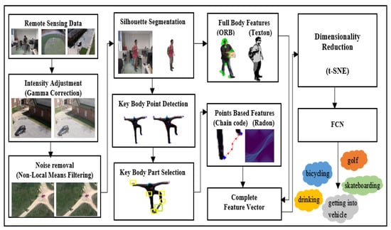
Figure 1.
The architecture of the proposed HOI system.
3.1. Image Pre-Processing
The first step of the proposed system is to pre-process the images. This is important especially in the case of remote sensing aerial imagery because videos collected through UAV and drone-based cameras usually have lower resolutions, noise, and illumination variation. Hence, all input images have been normalized first. In other words, the intensity values of all images have been adjusted using gamma correction and then noise has been removed from the images using the non-local means filtering technique. Figure 2 shows the results of these two operations on an aerial image.
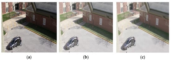
Figure 2.
Pre-processing results on the VIRAT dataset, including (a) original image, (b) intensity-adjusted image, and (c) smooth image.
3.1.1. Intensity Value Adjustment
Intensity value adjustment has been used to improve the contrast of the image and to make it clearer. The proposed system uses gamma correction for this purpose. This technique controls the overall brightness of an image. Several images in the used datasets look either bleached out or too dark. Gamma correction, also known as the Power Law transform, improves the quality of such images. The output gamma-corrected image has been obtained by adjusting the intensity values i of pixels x of an input image I using Equation (1):
where is the gamma value that can shift the image towards the darker end of the spectrum if it is set less than 1. However, if the gamma value is greater than 1, the image will appear lighter. A gamma value of 1 will not affect the input image.
3.1.2. Noise Removal
The technique of non-local means filtering has been used to remove noise from the images. It differs from a local means filter in such a way that instead of replacing the value of a pixel with the average of the values of its surrounding pixels, a non-local means filter replaces the value of a pixel with the weighted average of all the pixels in the image. Moreover, the weights of the image pixels are calculated on the basis of their similarity with the target pixel. A pixel in the denoised image u(p) at point p after applying the non-local means denoising technique on a pixel at point q in the original image v(q) has been defined by Equation (2).
where f(p, q) is the weight and C(p) is a normalization factor defined by Equation (3).
3.2. Silhouette Segmentation
Image segmentation refers to the process of dividing an image into regions, also called super-pixels. After pre-processing the images, the proposed method applies image segmentation to extract the desired silhouettes. Felzenszwalb’s algorithm [27] has been utilized for super-pixel segmentation. This method uses a graph-based representation of the image to decide where to place a boundary between two regions. An important characteristic of this method is that it ignores detail in high-variability regions to preserve detail in low-variability image regions.
As shown in Figure 3, Felzenszwalb’s algorithm divides the given image into multiple regions. To extract the desired silhouette, a region merging technique, which is quite similar to the one proposed by Xu et al. [28], has been employed. Using this technique, similar and adjacent regions have been merged based on their similarity until three large regions have been obtained. In other words, multiple small regions are recursively merged to form three larger regions: the human, the object, and the background. For this merging, four types of features have been extracted from each region, namely mean, covariance, scale-invariant feature transform (SIFT), and speeded-up robust features (SURF). Any two adjacent regions have been merged if the similarity between the values of these features of the two regions is above a certain threshold. The similarity has been computed using Equation (4).
where i and j are any two regions and represents the adjacency relation between them. If these two regions are adjacent, the value of is 1; otherwise, it is 0. , and are the similarities between the mean, covariance, SIFT, and SURF features of the two regions. Algorithm 1 explains this region-merging process in detail.
| Algorithm 1: Segmentation and Region Merging |
| Input: Image X = [x1,…xn] Output: Cluster centers of merged regions C = [c1, c2, c3] Repeat Regions ← Felzenszwalb’s algorithm (X) %Extract features% For i in len(Regions): Mean[i]←Get_Mean(Regions[i]) Covar[i]←Get_Covariance(Regions[i]) SIFT[i]←Get_SIFT_descriptors(Regions[i]) SURF[i]←Get_SURF_descriptors(Regions[i]) End %Compute Similarity% For i,j in len(Regions): ← sim(Mean[i], Mean[j]) ← sim(Covar[i], Covar[j]) ← sim(SIFT[i], SIFT[j]) ← sim(SURF[i], SURF[j]) End If >= threshold: NewRegion = MergeRegions(Region[i],Region[j]) End Until all images have been segmented Return C = [c1,c2,c3] |
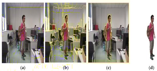
Figure 3.
Image segmentation results on SYSU 3D HOI dataset, including (a) original image, (b) image segmentation, (c) merged regions, and (d) extracted silhouette.
3.3. Automated Parts-Based Model
After extracting the full-body silhouette, five key body points have been identified using an approach similar to the one suggested by Dargazany et al. [29]. The segmented silhouette has been converted into a binary silhouette and then its contour has been obtained. Further, a convex hull has been drawn around the contour. Points on the convex hull that were also part of the original contour have been obtained. Only five such points have been chosen since having more than one point on the same body part is useless. In cases where multiple points were detected on the same body part, only one is selected through a point elimination technique based on Euclidean distance. Furthermore, a sixth point has been obtained by finding the centroid of the contour. The formula for computing the centroid C of a contour is given by Equation (5).
where , , and are image moments. The image moments are statistical parameters of an image, which are used to measure the distribution and intensities of different pixels. The image moments of an image can be calculated using Equation (6):
Using the obtained six points, six additional key points have been obtained. The midpoint of two key points has been found and a point on the contour lying closest to the obtained midpoint has been stored as an additional key point. For example, the right elbow lies between the head and the right hand. Hence, the midpoint of the right hand and the head is computed using Equation (7):
Then, the Euclidean distances between this midpoint and all other points lying on the human contour are calculated and the point having the minimum distance is selected as the right elbow point. Similarly, the hip joints are found by calculating the midpoints of the head and the feet. Likewise, the knee joints are identified by finding the midpoints of the torso and the feet. Each step of the process is shown in Figure 4.
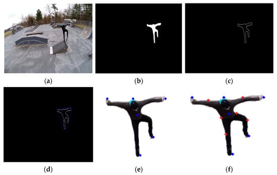
Figure 4.
Steps of human body points detection over the YouTube Aerial dataset, including (a) original image, (b) binary silhouette, (c) silhouette contour, (d) convex hull, (e) six key points, and (f) twelve key points.
Twelve key points have been identified using the binary human silhouettes. However, all twelve parts do not contribute to the overall interaction. Therefore, it is time-consuming and ineffective to extract features for all these parts. Instead, only five key points have been selected that are involved in a particular interaction. To compute the involvement score of each body part, the cosine similarity metric has been used, as shown in Equation (8). The cosine similarity metric finds the normalized dot product of the two inputs. In other words, the cosine similarity judges orientation and not magnitude. If any two vectors have the same orientation, they will have a cosine similarity of 1. On the other hand, if they have different orientations, i.e., the angle between any two vectors is 90°, they will have a similarity of 0.
where A is the centroid of the detected object and B is any of the twelve key points. In this way, the cosine similarity score of each body part has been computed and then the five body parts with the highest scores have been selected. Figure 5 shows the twelve initially detected points and then the five points that were selected based on cosine similarity. Table 2 shows the actual values of the similarity scores of the twelve body parts of the silhouette shown in Figure 5.
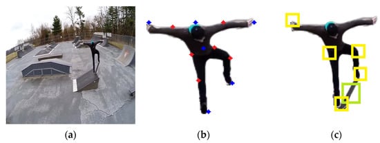
Figure 5.
Key-part selection over the YouTube Aerial Action dataset, including (a) original image, (b) twelve detected body parts, and (c) five selected parts.
Table 2.
Cosine similarity scores of different body parts.
The proposed automated parts-based model consists of these two stages of body-part detection and body-part selection. Each step of the process is described in detail in Algorithm 2.
| Algorithm 2: Automated Parts-Based Model |
| Input: HSS: segmented human silhouette Output: 12 body parts including head, left elbow, right elbow, left hand, right hand, torso, left hip, right hip, left knee, right knee, left foot, right foot: key_body_points (p1, p2, p3…p12) and selected parts: key_body_parts (p1, p2, p3, p4, p5). Repeat KeyBodyPoints ← [] % detecting 5 key points from convex hull% For i = 1 to N do contour ← Getcontour (HSS) Convex hull ← DrawConvexhull (contour) For point on Convex hull do If point in contour do KeyBodyPoints.append (point) End End |
| %detecting 6th key point from contour center% Center ← GetContourcenter (contour) KeyBodyPoints.append (Center) %detecting 6 additional key points% LE ← FindMidpoint (KeyBodyPoints [0], KeyBodyPoints [1]) lelbow ← Findclosestpointoncontour (LE) RE ← FindMidpoint (KeyBodyPoints [2], KeyBodyPoints [1]) relbow ← Findclosestpointoncontour (RE) LH ← FindMidpoint (KeyBodyPoints [3], KeyBodyPoints [1]) lhip ← Findclosestpointoncontour (LH) RH ← FindMidpoint (KeyBodyPoints [4], KeyBodyPoints [1]) rhip ← Findclosestpointoncontour (RH) LK ← FindMidpoint (KeyBodyPoints [3], KeyBodyPoints [5]) lknee ← Findclosestpointoncontour (LK) RK ← FindMidpoint (KeyBodyPoints [4], KeyBodyPoints [5]) rknee ← Findclosestpointoncontour (RK) KeyBodyPoints.append (lelbow, relbow, lhip, rhip, lknee, rknee) End return key_body_points (p1, p2, p3…p12) Scores ← [] For point in key_body_points do Score ← CosineSimilarity(point, object) Scores.append (score) End key_body_parts ← Get_top_5_points (Scores) Return key_body_parts (p1, p2, p3, p4, p5) |
3.4. Multi-Scale Feature Extraction
This section describes the extraction process of multi-scale features used in the proposed system. Four types of multi-scale features have been extracted, including ORB descriptors and texton maps for full-body silhouettes, and Radon transforms and 8-chain Freeman codes for key body parts. Algorithm 3 shows an overview of the multi-scale feature extraction step.
| Algorithm 3: Multi-Scale Feature Extraction |
| Input: N: full body silhouettes and five key body points Output: combined feature vector (f1, f2, f3…fn) % initiating feature vector for remote sensing HOI classification % FeatureVector ← [] F_vectorsize ← GetVectorsize () % loop on extracted human silhouettes % J ← len(silhouettes) For i = 1:J % extracting ORB and Texton features % ORB ← GetORBdescriptor (silhouette[i])) Texton ← GetTextonMap (silhouette[i])) FeatureVector.append (ORB, Texton) % loop on five key points % For i = 1:5 % extracting Chain Code and Radon features % Code ← GetChainCode(i, i + 1) Radon ← GetRadonTransform (silhouette, i) FeatureVector.append (Code, Radon) End End Feature-vector ← Normalize (FeatureVector) return feature vector (f1, f2, f3…fn) |
3.4.1. ORB Features
Oriented FAST and rotated BRIEF (ORB) [30] is a fast robust local feature detector. It is based on the features from the accelerated segment test (FAST) key point detector and is a modified version of the visual descriptor called Binary Robust Independent Elementary Features (BRIEF). ORB is scale- and rotation-invariant. It basically rotates BRIEF according to the orientation of key points detected using FAST. In other words, it uses the orientation of an image patch θ, computed using Equation (9), to find its rotated version.
where and are image moments. While the key point orientation θ remains consistent across different views, the correct set of points is used to compute its feature descriptor. Two full-body silhouettes and the key feature points detected by ORB are shown in Figure 6.
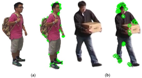
Figure 6.
ORB feature points of silhouettes from the SYSU 3D HOI and VIRAT Video datasets, including (a) wearing backpack—full silhouette (left) and its ORB feature points (right) and (b) carrying an object—full silhouette (left) and its ORB feature points (right).
3.4.2. Texton Maps
Textons can be defined as the fundamental micro-structures in images [31]. As explained by Julesz et al. [32], we can understand textons as atoms whose protons, neutrons, and electrons are image bases. These textons can therefore be used to represent many different pixel relationships in an image. This is often needed when performing image texture analysis. Texton maps are obtained by convolving the images with filters. Three types of filter banks are commonly used, including the Leung Malik (LM) filter bank, the Schmid (S) bank, and the maximum response (MR) bank.
This paper uses the LM filter bank [33] for obtaining the texton maps of the given full-body silhouettes. The LM filter bank provides 48 filters, including 2 Gaussian derivative filters at 6 orientations and 3 scales, 8 Laplacian of Gaussian (LOG) filters, and 4 Gaussian filters. At each pixel, a response vector of size equal to the number of filters in the filter bank is formed by storing the response from each filter, as shown in Equation (10).
where is the original image and is the filter bank. After convolution, the resulting filter response vectors will contain the filter responses obtained by convolving the input image pixels with each filter in the filter bank. These response vectors are divided into k clusters using the k-means clustering algorithm, where each cluster represents a texture class. Figure 7 shows two silhouettes and their texton maps.
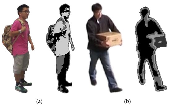
Figure 7.
Texton maps of silhouettes from SYSU 3D HOI and VIRAT Video datasets: (a) wearing backpack—full silhouette (left) and its texton map (right) and (b) carrying an object—full silhouette (left) and its texton map (right).
3.4.3. Radon Transform
The Radon transform is a mapping from the Cartesian rectangular coordinates (x, y) to the polar coordinates (ρ, θ). The resulting projection is the sum of the intensities of the pixels in each direction, i.e., a line integral. The Radon transform R(ρ, θ) of an image f(x, y) can be obtained using Equation (11):
where is the angle between x and y, computed using Equation (12).
Similarly, is the distance between x and y, computed using Equation (13).
The proposed system extracts an image window of size 30 × 30 around each key point and obtains its Radon transform. Figure 8 shows two such windows and their Radon transforms. In Figure 8a, a 30 × 30 window has been drawn around the right-hand joint and its Radon transform has been obtained. Similarly, in Figure 8b, a 30 × 30 window has been drawn around the left-foot joint and its Radon transform has been obtained.
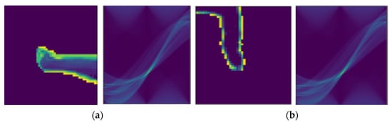
Figure 8.
Radon transforms of a silhouette from the VIRAT Video dataset, including (a) a window around the right hand (left) and its Radon transform (right) and (b) a window around the left foot (left) and its Radon transform (right).
3.4.4. Eight-Chain Freeman Codes
Freeman chain codes are commonly used as shape descriptors since they can represent the boundary of a given shape using the coordinates of the starting point and the direction code of the boundary point. It is often used to represent the boundary of the curve and area in the fields of image processing, computer graphics, and pattern recognition. In simple words, it is a coded representation of boundaries where the direction of the boundary is used as the basis for coding.
Commonly used chain codes are divided into four- or eight-connected chain codes according to the number of adjacent directions of central pixels. There are four adjacent points of four-connected chain codes, which are above, below, left, and right of the center point, respectively. The eight-connected chain code adds four diagonal directions to the four-connected chain code. Since there are eight adjacent points around any pixel, the eight-connected chain code exactly matches the actual situation of the pixel, which can accurately describe the central pixel and its information about adjacent points. Therefore, the use of eight-connected chain codes is relatively larger.
The proposed method extracts Freeman chain codes for straight lines between every two key body points. Figure 9a shows the eight code values and the directions they represent. Figure 9b shows the visualization of the chain code for a straight line between the two human feet. Similarly, Figure 9c visualizes the code for a straight line between the right hand and the right foot.
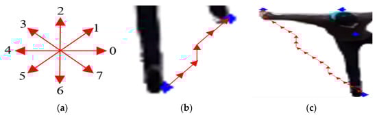
Figure 9.
Freeman chain code feature showing (a) eight possible directions, (b) the chain code of a straight line between the right and the left foot, and (c) the chain code of a straight line between the right foot and the right hand.
3.5. Dimensionality Reduction: t-SNE
After extracting the four types of features from all the images, they have been concatenated and added as descriptors of each interaction class. However, this results in a very high-dimensional feature vector. The size of the ORB descriptor is 200 × 32 or 1 × 6400 and that of the texton feature is 1 × 54. The size of each Radon transform feature is 254 × 180 or 1 × 45,720 and that of each chain code is 1 × 20. However, since Radon transforms and chain codes are obtained for at least five key points per input silhouette, these feature sizes are multiplied by 5. Therefore, the combined feature vector is of the size 1 × 235,154 for each input image. Hence, dimensionality reduction becomes an important requirement at this stage. There are two ways of doing this: keeping the features with maximum variance and eliminating redundant features or transforming the original set of features into a smaller set of new features with almost the same variance as the original ones. The t-distributed Stochastic Neighbor Embedding (t-SNE) technique [34] employed in this research is a non-linear dimensionality reduction method that uses the latter approach as it transforms the 235,154 columns containing different feature values into 3 new columns. As the name indicates, this method is based on random probability and focuses only on retaining the variance of the neighboring points. The number of neighboring points, also known as perplexity, was set to 75 and the number of iterations was set to 5000 during the experiments performed in this study.
The t-SNE is a powerful technique that preserves both the local and global structure of the data. In other words, after applying dimensionality reduction through t-SNE, the obtained low-dimensional map contains as much of the significant structure as in the original high-dimensional data. The t-SNE technique works by constructing a probability distribution over pairs of high-dimensional objects. Similar objects are given high probability while dissimilar points are given low probability. The density of all points (xj) is measured under this Gaussian distribution and is renormalized for all points. This results in a set of probabilities (Pij) for all points, which can be represented by Equation (14).
The next step of the process is to define a similar probability distribution over the points in the low-dimensional map. However, a Student t-distribution with one degree of freedom, which is also known as the Cauchy distribution, is used this time instead of a Gaussian distribution. This gives a second set of probabilities (Qij) in the low-dimensional space, which can be represented by Equation (15).
After obtaining the two sets of probabilities, their distributions are measured using Kullback–Liebler divergence (KL), as shown in Equation (16). If the value of the KL divergence is low, it means that the two distributions are close to one another. In other words, if the two distributions are identical, the value of KL divergence will be 0.
Lastly, the KL cost function is minimized using gradient descent. After optimization, a t-SNE map is obtained that reflects the similarities between the high-dimensional inputs. Figure 10 shows the t-SNE plots for the three datasets used in this research.
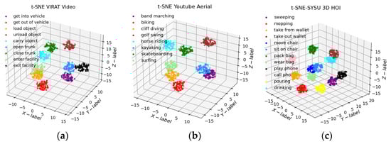
Figure 10.
A few examples of t-SNE dimensionality reduction results over the (a) VIRAT Video dataset, (b) YouTube Aerial dataset, and (c) SYSU 3D HOI dataset.
3.6. Fully Convolutional Network
This section discusses the use of a fully convolutional network (FCN) with a softmax layer for the classification of HOI interactions. Unlike a convolutional neural network (CNN), FCN does not need a fixed input size because, in an FCN model, the fully connected layers of a CNN model are replaced by convolution layers. This is useful since the requirement of fixed input size needs input images to be resized, which can cause a loss of resolution. This becomes an issue when the target human or object constitutes only a small section of the image, as in the case of aerial images.
Moreover, image classification networks are usually trained on square images. Therefore, if the input image is not square, it is common to extract either a square region from the center or to resize the width and height of the image to make it a square. In the first case, important features that are not in the center of the image may be missed. In the second case, the image will be distorted because the performed scaling operation is non-uniform. Figure 11 shows the basic architecture of an FCN model.
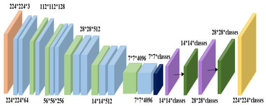
Figure 11.
Basic architecture of a fully convolutional network.
The FCN model used in the proposed system consisted of two 2D convolution layers with 64 filters and the RELU activation function. Each convolution layer was followed by a dropout layer of 0.2 and a batch normalization layer. These two layers ensure regularization, which prevents overfitting and reduces the convergence time. Moreover, activation layers are used to incorporate non-linearity. Then, a global max-pooling layer was used. Finally, for computing the classification score, a softmax layer was added to this FCN model.
4. Experimental Results
This section describes the three publicly available datasets that have been used to validate the proposed system. The description is followed by the implementation details and the results of different experiments performed on the three datasets. FCN has been used and the proposed system has been evaluated using the Leave One Subject Out (LOSO) cross-validation technique. In this technique, each subject is used once as the test set. It is a special type of k-fold cross-validation, in which the number of folds is equal to the number of instances in the dataset. The proposed FCN model has been developed in Python 3.8 using Jupyter Notebook. Python’s deep learning library, Keras, has been used as it provides the different layers for convolution, batch normalization, flattening, max-pooling, and softmax. Moreover, the Adam optimizer and categorical cross-entropy loss have been used. The proposed model has been trained for 50 epochs. All the processing and experiments were performed on a Windows 10 operating system having 16-GB RAM, and a processor of core-i7-7500U CPU @ 2.70 GHz. Finally, the performance of the proposed system is also compared with the accuracies of other state-of-the-art systems tested on these datasets.
4.1. Dataset Description
Two remote sensing datasets called VIRAT Video [35] and YouTube Aerial [36] and one RGBD dataset called SYSU 3D HOI [37] have been used for experimentation. Table 3 provides a brief summary of all three datasets, while detailed descriptions and some sample frames of each dataset are given in the following subsections.
Table 3.
A summary of the datasets used for experimentation.
4.1.1. VIRAT Video Dataset
The video and image retrieval and analysis tool (VIRAT) Video dataset is a large-scale surveillance video dataset designed for event recognition algorithms but has been used for testing human–vehicle interaction recognition systems as well [38]. It contains videos collected from both stationary ground cameras and moving aerial vehicles. The videos contain both human–human and human–object interactions. The nine HOI interactions include loading an object, unloading an object, opening a trunk, closing a trunk, getting into a vehicle, getting out of a vehicle, carrying an object, entering a facility, and exiting a facility. This is a challenging dataset since the aerial videos have very fast camera motion and have been captured from large heights. Some sample frames are shown in Figure 12.
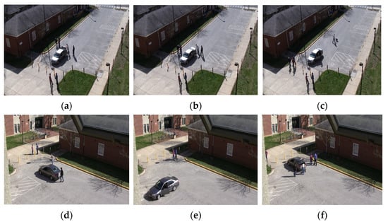
Figure 12.
A few samples of the VIRAT Video dataset, including (a) opening trunk, (b) closing trunk, (c) entering into vehicle, (d) carrying an object, (e) getting out of vehicle, and (f) loading an object.
4.1.2. YouTube Aerial Dataset
The YouTube Aerial dataset contains various drone videos available on YouTube, corresponding to eight actions of the UCF101 dataset [39]. These eight HOI interactions include band marching, biking, cliff-diving, golf-swing, horse-riding, kayaking, skateboarding, and surfing. This is a challenging dataset since the aerial videos contain fast camera motion and have been captured from variable heights. There are 50 videos of each interaction. Some sample frames are shown in Figure 13.
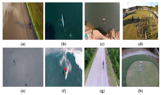
Figure 13.
A few samples of the YouTube Aerial dataset, including (a) horse-back riding, (b) kayaking, (c) cliff-diving, (d) band marching, (e) skateboarding, (f) surfing, (g) cycling, and (h) golf.
4.1.3. SYSU 3D HOI Dataset
The Sun Yat-sen University (SYSU) 3D HOI dataset provides RGB, depth, and skeleton data. It has been recorded using a Kinect sensor. It contains twelve human–object interactions performed by 40 participants. These interactions include sweeping, mopping, taking from wallet, taking out wallet, moving chair, sitting in chair, packing backpacks, wearing backpacks, playing on phone, calling phone, pouring, and drinking. There are 480 videos of durations ranging from 1.9 to 21 s. Some sample frames are shown in Figure 14.
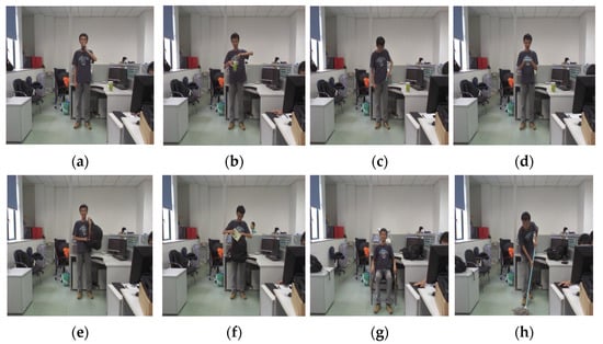
Figure 14.
A few samples of the SYSU 3D HOI dataset, including (a) drinking, (b) pouring, (c) taking out wallet, (d) playing on phone, (e) wearing backpack, (f) packing backpack, (g) sitting in chair, and (h) mopping.
4.2. Experiment I: Interaction Classification Accuracies
The interaction classification accuracies have been expressed in terms of confusion matrices in Figure 15, Figure 16 and Figure 17. It can be seen that the system achieves average accuracies of 82.55%, 86.63%, and 91.68% over the VIRAT Video, YouTube Aerial, and SYSU 3D HOI datasets, respectively.
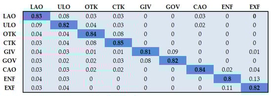
Figure 15.
Classification accuracy over the VIRAT Video dataset. LAO = loading an object, ULO = unloading an object, OTK = opening trunk, CLK = closing trunk, GIV = getting into vehicle, GOV = getting out of vehicle, CAO = carrying an object, ENF = entering a facility, EXF = exiting a facility.
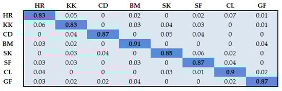
Figure 16.
Classification accuracy over the YouTube Aerial dataset. HR = horse riding, KK = kayaking CD = cliff-diving BM = band marching, SK = skateboarding, SF = surfing, CL = cycling, GF = golf.
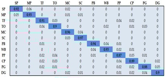
Figure 17.
Classification accuracy over the SYSU 3D HOI dataset. SP = sweeping, MP = mopping, TF = taking from wallet, TO = taking out wallet, MC = moving chair, SC = sitting in chair, PB = packing backpacks, WB = wearing backpacks, PP = playing on phone, CP = calling phone, PG = pouring, DG = drinking.
4.3. Experiment II: Accuracy and Loss Plots
The accuracy and loss plots of the training and validation sets from the VIRAT Video, Youtube Aerial, and SYSU 3D HOI datasets are shown in Figure 18, Figure 19 and Figure 20, respectively. It can be seen that the model’s accuracy increases and loss decreases with increasing epochs.
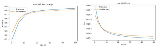
Figure 18.
Model accuracy and loss plots for the VIRAT Video dataset.
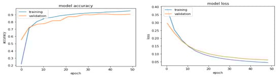
Figure 19.
Model accuracy and loss plots for the YouTube Aerial dataset.
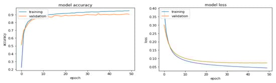
Figure 20.
Model accuracy and loss plots for the SYSU 3D HOI dataset.
4.4. Experiment II: Part-Based Model Detection
Accurate detection of human body parts leads to better classification results. Hence, the class-wise accuracies of the twelve body parts detected using the proposed key-point detection algorithm have also been discussed. First, the Euclidean distance D between the ground truth value and the detected value of each key body part is computed using Equation (17).
where DV is the detected value and GT is the ground truth value of a body part i. Based on its distance from the ground truth value, the accuracy of the detected body part is computed using Equation (18).
where Th is the threshold value, which was set to 15, and n represents the total sample frames of each interaction class. Table 4, Table 5 and Table 6 show the average body part detection accuracies achieved by the proposed system over the VIRAT Video, YouTube Aerial, and SYSU 3D HOI datasets, respectively.
Table 4.
Results of body part detection over the VIRAT Video dataset.
Table 5.
Results of body part detection over the YouTube Aerial dataset.
Table 6.
Results of body part detection over the SYSU 3D HOI dataset.
4.5. Experiment III: Comparison with Other Classifiers
In this section, accuracy metrics including precision, recall, and F1 measure have been computed using Equations (19)–(21), respectively.
The performances of the artificial neural network (ANN) and CNN have been compared with that of the FCN in terms of the above-mentioned accuracy metrics and time complexities. The structures and details of these ANN and CNN models have been described in detail in [40,41], respectively. The optimized feature vectors of all three datasets have been fed into ANN, CNN, and FCN models. Table 7 shows the results over the VIRAT Video dataset, Table 8 shows the results over the YouTube Aerial dataset, and Table 9 shows the results over the SYSU 3D HOI dataset. Table 10 shows the running times of all three models over the three datasets. The mean running times have been obtained over five instances with a 95% confidence interval. The results show that the FCN achieves better scores than the other two classifiers and is faster as well.
Table 7.
Comparison with well-known classifiers in terms of precision, recall, and F1 measure over VIRAT Video dataset.
Table 8.
Comparison with well-known classifiers in terms of precision, recall, and F1 measure over YouTube Aerial dataset.
Table 9.
Comparison with well-known classifiers in terms of precision, recall, and F1 measure over SYSU HOI 3D dataset.
Table 10.
Time complexity of different classifiers.
4.6. Experimentation IV: Comparison of the Proposed System with State-of-the-Art Techniques
This section compares the classification accuracy of the proposed system with that of the existing state-of-the-art methods on the three datasets that have been used in this research. The classification accuracy is computed by dividing the number of correct predictions by the total number of predictions that were made by the classifier, as shown in Equation (22). Similarly, the classification error can be calculated by dividing the number of incorrect predictions by the total number of predictions made by the classifier, as shown in Equation (23). For the proposed model, a 95% confidence interval has also been calculated using Equation (24). Table 11 shows that the proposed system outperforms many other state-of-the-art methods.
Table 11.
Comparison of the state-of-the-art methods with the proposed system.
5. Discussion
The proposed HOI recognition system achieved impressive human pose estimation and human–object interaction detection results over ground and aerial imagery. In this approach, all input images were pre-processed to improve their quality. Then, humans and objects were segmented out from the images. Using these segmented human silhouettes, twelve key body parts were identified. Then, only five of these points were selected based on their cosine similarity score with the target object. Next, multi-scale features were extracted, including ORB descriptors, texton maps, Radon transforms, and eight-chain Freeman codes. These features were combined and then dimensionality reduction was applied. Lastly, the interactions were classified using FCN.
The results and analysis of the proposed HOI detection system are presented as follows. The mean human body part detection rate is 85.53% for the VIRAT Video dataset, 86.14% for the YouTube Aerial dataset, and 93.02% for the SYSU 3D HOI dataset. Moreover, the mean interaction classification accuracy is 82.55% over the VIRAT Video dataset, 86.63% for the YouTube Aerial dataset, and 91.68% for the SYSU 3D HOI dataset. These results are better than those achieved by the existing state-of-the-art methods. Several factors contribute to the better performance of the proposed system as compared to the existing methods. Unlike those methods which have used raw images as input, the proposed system has been trained and evaluated on pre-processed images. Moreover, subtracting the backgrounds from the images also removes the redundant background features, which would have otherwise contributed to the overall classification process. While other systems used limited features, the proposed approach used multi-scale features, which have been extracted from full humans as well as their key body parts. Knowing the exact body parts that were involved made it easier for the classifier to detect which interaction was performed. Finally, t-SNE optimized the high-dimensional dataset. Since the combined feature vector was of the size 1 × 235,154 for each input image, without dimensionality reduction, the model would become so complex that it would be non-trainable.
The automated part-based model proposed in this paper extracts the twelve key human body parts. Experimental results show that the model achieves a very high detection rate in the case of the SYSU 3D HOI dataset but considerably lower detection rates for the two aerial datasets. This is because humans make up only a small part of the overall aerial images. Hence, it becomes difficult to identify their body parts. Moreover, the proposed system shows slightly lower accuracy rates for aerial datasets. This is due to the low image resolutions and fast camera motions that are almost always associated with remote sensing imagery.
Despite these limitations, the proposed system can be applied in real-life scenarios that involve surveillance and monitoring applications. Thus far, this model has only been tested on publicly available datasets and not real-time data. However, for its practical usage, ground and aerial cameras can be added to it to acquire real-time human–object interaction videos. Figure 21 shows one such scenario where surveillance and monitoring is needed. Each person who enters the area is verified and then continuously monitored. His interactions with the objects in his surroundings are recognized and matched with an available list of forbidden interactions. If any of the recognized interactions is forbidden, the surveillance system raises an alarm.
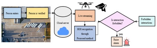
Figure 21.
An example of practical usage of the proposed HOI recognition system for surveillance.
6. Conclusions
This research provides an efficient image segmentation technique, a simple yet effective key point detection and body part selection method, and a robust system for HOI recognition that has been validated on complex human movements, varying postures, and cluttered backgrounds. To pre-process the input images, the techniques of gamma correction and non-local means filtering have been used. For image segmentation, an improved version of the Felzenszwalb algorithm has been employed. Using these segmented silhouettes, twelve key body points have been identified, five of which have been utilized for feature extraction. Four types of features have been extracted, including ORB, texton maps, Radon transforms, and Freeman chain codes. For data optimization, t-SNE has been explored, and for classification, FCN has been used. As shown in the experimentation section, the proposed system has shown better performance over challenging datasets than many existing methods. This system can find its application in various fields ranging from healthcare, assisted living, and sports to education, training, and surveillance. Moreover, with slight modifications, such as the addition of UAV cameras and multi-vision sensors, the proposed system can be used for real-time environments.
6.1. Theoretical Implications
The proposed system efficiently detects human–object interactions in complex and challenging remote sensing and RGBD video datasets. The reason for validating the system using multiple and varying datasets is to prove the general applicability and overall efficiency of the proposed approach. Moreover, the task of HOI recognition using remote sensing data is an under-researched area in the field of computer vision. Hence, this article will suggest new directions for research in this regard. The proposed system can be used for research on HOI recognition in videos from sports, healthcare, e-learning, and surveillance datasets.
6.2. Research Limitations
The proposed HOI recognition system has been tested on two aerial datasets. The videos in the YouTube Aerial dataset are clearer and mostly captured from a lower height. On the other hand, the VIRAT Video dataset poses other problems due to fast camera motion and extreme heights. The target humans are very small in size, making the proposed key point detection method less efficient. Hence, the system’s performance was affected in such situations, as shown by the relatively poor results on the VIRAT Video dataset. In the future, we aspire to work on this problem by modifying the key point detection algorithm and using new feature descriptors that should lead to better results.
Author Contributions
Conceptualization, M.W. and A.J.; methodology, M.W. and Y.Y.G.; software, M.W., S.A.A. and T.a.S.; validation, M.W., Y.Y.G. and J.P.; formal analysis, T.a.S., S.A.A. and J.P.; resources, Y.Y.G., T.a.S. and J.P.; writing—review and editing, M.W., T.a.S. and J.P.; funding acquisition, Y.Y.G., M.W., S.A.A. and J.P. All authors have read and agreed to the published version of the manuscript.
Funding
This research was supported by a grant (2021R1F1A1063634) from the Basic Science Research Program through the National Research Foundation (NRF), funded by the Ministry of Education, Republic of Korea.
Institutional Review Board Statement
Not applicable.
Informed Consent Statement
Not applicable.
Data Availability Statement
Not applicable.
Conflicts of Interest
The authors declare no conflict of interest.
References
- Fraser, B.T.; Congalton, R.G. Monitoring Fine-Scale Forest Health Using Unmanned Aerial Systems (UAS) Multispectral Models. Remote Sens. 2021, 13, 4873. [Google Scholar] [CrossRef]
- Mahmood, M.; Jalal, A.; Kim, K. WHITE STAG Model: Wise Human Interaction Tracking and Estimation (WHITE) using Spatio-temporal and Angular-geometric (STAG) Descriptors. Multimed. Tools Appl. 2020, 79, 6919–6950. [Google Scholar] [CrossRef]
- Liu, H.; Mu, T.; Huang, X. Detecting human—object interaction with multi-level pairwise feature network. Comput. Vis. Media 2020, 7, 229–239. [Google Scholar] [CrossRef]
- Cheong, K.H.; Poeschmann, S.; Lai, J.W.; Koh, J.M.; Acharya, U.R.; Yu, S.C.M.; Tang, K.J.W. Practical Automated Video Analytics for Crowd Monitoring and Counting. IEEE Access 2019, 7, 183252–183261. [Google Scholar] [CrossRef]
- Nida, K.; Gochoo, M.; Jalal, A.; Kim, K. Modeling Two-Person Segmentation and Locomotion for stereoscopic Action Identification: A Sustainable Video Surveillance System. Sustainability 2021, 13, 970. [Google Scholar]
- Tahir, B.; Jalal, A.; Kim, K. IMU sensor based automatic-features descriptor for healthcare patient’s daily life-log recognition. In Proceedings of the IBCAST 2021, Bhurban, Pakistan, 12–16 August 2022. [Google Scholar]
- Javeed, M.; Jalal, A.; Kim, K. Wearable sensors based exertion recognition using statistical features and random forest for physical healthcare monitoring. In Proceedings of the IBCAST 2021, Bhurban, Pakistan, 12–16 August 2022; pp. 512–517. [Google Scholar]
- Jalal, A.; Sharif, N.; Kim, J.T.; Kim, T.-S. Human activity recognition via recognized body parts of human depth silhouettes for residents monitoring services at smart homes. Indoor Built Environ. 2013, 22, 271–279. [Google Scholar] [CrossRef]
- Cafolla, D. A 3D visual tracking method for rehabilitation path planning. In New Trends in Medical and Service Robotics; Springer: Cham, Switzerland, 2019; pp. 264–272. [Google Scholar]
- Chaparro-Rico, B.D.; Cafolla, D. Test-retest, inter-rater and intra-rater reliability for spatiotemporal gait parameters using SANE (an eaSy gAit aNalysis systEm) as measuring instrument. Appl. Sci. 2020, 10, 5781. [Google Scholar] [CrossRef]
- Jalal, A.; Kamal, S. Real-time life logging via a depth silhouette-based human activity recognition system for smart home services. In Proceedings of the AVSS 2014, Seoul, Korea, 26–29 August 2014; pp. 74–80. [Google Scholar]
- Jalal, A.; Mahmood, M. Students’ Behavior Mining in E-Learning Environment Using Cognitive Processes with Information Technologies. Educ. Inf. Technol. 2019, 24, 2797–2821. [Google Scholar] [CrossRef]
- Wan, B.; Zhou, D.; Liu, Y.; Li, R.; He, X. Pose-Aware Multi-Level Feature Network for Human Object Interaction Detection. In Proceedings of the ICCV 2019, Seoul, Korea, 27 October–2 November 2019; pp. 9468–9477. [Google Scholar]
- Yan, W.; Gao, Y.; Liu, Q. Human-object Interaction Recognition Using Multitask Neural Network. In Proceedings of the ISAS 2019, Albuquerque, NM, USA, 21–25 July 2019; pp. 323–328. [Google Scholar]
- Wang, T.; Yang, T.; Danelljan, M.; Khan, F.S.; Zhang, X.; Sun, J. Learning Human-Object Interaction Detection Using Interaction Points. In Proceedings of the CVPR 2020, Virtual, 14–19 June 2020; pp. 4116–4125. [Google Scholar]
- Gkioxari, G.; Girshick, R.; Dollár, P.; He, K. Detecting and Recognizing Human-Object Interactions. In Proceedings of the CVPR 2018, Salt Lake City, UT, USA, 18–22 June 2018; pp. 8359–8367. [Google Scholar]
- Li, Y.L.; Liu, X.; Lu, H.; Wang, S.; Liu, J.; Li, J.; Lu, C. Detailed 2D-3D Joint Representation for Human-Object Interaction. In Proceedings of the CVPR 2020, Virtual, 14–19 June 2020; pp. 10163–10172. [Google Scholar]
- Jin, Y.; Chen, Y.; Wang, L.; Yu, P.; Liu, Z.; Hwang, J.N. Is Object Detection Necessary for Human-Object Interaction Recognition? arXiv 2021, arXiv:2107.13083. [Google Scholar]
- Girdhar, R.; Ramanan, D. Attentional Pooling for Action Recognition. In Proceedings of the NIPS 2017, Long Beach, CA, USA, 4–9 December 2017. [Google Scholar]
- Gkioxari, G.; Girshick, R.; Malik, J. Contextual Action Recognition with R*CNN. In Proceedings of the ICCV 2015, Santiago, Chile, 7–13 December 2015; pp. 1080–1088. [Google Scholar]
- Shen, L.; Yeung, S.; Hoffman, J.; Mori, G.; Fei, L. Scaling human-object interaction recognition through zero-shot learning. In Proceedings of the WACV 2018, Lake Tahoe, NV, USA, 12–15 March 2018; pp. 1568–1576. [Google Scholar]
- Yao, B.; Li, F.-F. Recognizing Human-Object Interactions in Still Images by Modeling the Mutual Context of Objects and Human Poses. IEEE Trans. Pattern Anal. Mach. Intell. 2012, 34, 1691–1703. [Google Scholar] [PubMed]
- Meng, M.; Drira, H.; Daoudi, M.; Boonaert, J. Human-object interaction recognition by learning the distances between the object and the skeleton joints. In Proceedings of the International Conference and Workshops on Automatic Face and Gesture Recognition 2015, Ljubljana, Slovenia, 4–8 May 2015; pp. 1–6. [Google Scholar]
- Qi, S.; Wang, W.; Jia, B.; Shen, J.; Zhu, S.C. Learning Human-Object Interactions by Graph Parsing Neural Networks. In Proceedings of the ECCV 2018, Munich, Germany, 8–14 September 2018; pp. 407–423. [Google Scholar]
- Fang, H.S.; Cao, J.; Tai, Y.W.; Lu, C. Pairwise Body-Part Attention for Recognizing Human-Object Interactions. In Proceedings of the ECCV 2018, Munich, Germany, 8–14 September 2018; pp. 51–67. [Google Scholar]
- Mallya, A.; Lazebnik, S. Learning Models for Actions and Person-Object Interactions with Transfer to Question Answering. In Proceedings of the CVPR, Virtual, 14–19 June 2020; pp. 414–428. [Google Scholar]
- Felzenszwalb, P.F.; Huttenlocher, D.P. Efficient Graph-Based Image Segmentation. Int. J. Comput. Vis. 2004, 59, 167–181. [Google Scholar] [CrossRef]
- Xu, X.; Li, G.; Xie, G.; Ren, J.; Xie, X. Weakly Supervised Deep Semantic Segmentation Using CNN and ELM with Semantic Candidate Regions. Complexity 2019, 2019, 1–12. [Google Scholar] [CrossRef]
- Dargazany, A.; Nicolescu, M. Human Body Parts Tracking Using Torso Tracking: Applications to Activity Recognition. In Proceedings of the ITNG 2012, Las Vegas, NV, USA, 16–18 April 2012; pp. 646–651. [Google Scholar]
- Rublee, E.; Rabaud, V.; Konolige, K.; Bradski, G. ORB: An efficient alternative to SIFT or SURF. In Proceedings of the ICCV 2011, Barcelona, Spain, 6–13 November 2011; pp. 2564–2571. [Google Scholar]
- Javed, Y.; Khan, M.M. Image texture classification using textons. In Proceedings of the ICET 2011, Islamabad, Pakistan, 5–6 September 2011; pp. 1–5. [Google Scholar]
- Julesz, B. Textons, the elements of texture perception, and their interaction. Nature 1981, 290, 91–97. [Google Scholar] [CrossRef] [PubMed]
- Leung, T.; Malik, J. Representing and Recognizing the Visual Appearance of Materials using Three-dimensional Textons. In Proceedings of the ICCV 1999, Corfu, Greece, 20–25 September 1999; pp. 29–44. [Google Scholar]
- Maaten, L.; Hinton, G. Visualizing Data using t-SNE. J. Mach. Learn. Res. 2008, 9, 2579–2605. [Google Scholar]
- Oh, S.; Hoogs, A.; Perera, A.; Cuntoor, N.; Chen, C.C.; Lee, J.T.; Mukherejee, S.; Aggarwal, J.; Lee, H.; Swears, D.S.; et al. A large-scale benchmark dataset for event recognition in surveillance video. In Proceedings of the CVPR 2011, Colorado Springs, CO, USA, 21–23 June 2011; pp. 3153–3160. [Google Scholar]
- Sultani, W.; Shah, M. Human action recognition in drone videos using a few aerial training examples. Comput. Vis. Image Underst. 2021, 206, 103186. [Google Scholar] [CrossRef]
- Jalal, A.; Kamal, S.; Farooq, A.; Kim, D. A spatiotemporal motion variation features extraction approach for human tracking and pose-based action recognition. In Proceedings of the IEEE International Conference on Informatics, Electronics and Vision, Fukuoka, Japan, 15–18 June 2015. [Google Scholar]
- Lee, J.T.; Chen, C.C.; Aggarwal, J.K. Recognizing human-vehicle interactions from aerial video without training. In Proceedings of the CVPR Workshops 2011, Colorado Springs, CO, USA, 20–25 June 2011; pp. 53–60. [Google Scholar]
- Soomro, K.; Zamir, R.; Shah, M. Ucf101: A dataset of 101 human actions classes from videos in the wild. In Proceedings of the ICCV 2013, Sydney, Australia, 1–8 December 2013. [Google Scholar]
- Tahir, S.B.; Jalal, A.; Kim, K. IMU Sensor Based Automatic-Features Descriptor for Healthcare Patient’s Daily Life-Log Recognition. In Proceedings of the IEEE International Conference on Applied Sciences and Technology, Pattaya, Thailand, 1–3 April 2021. [Google Scholar]
- Waheed, M.; Javeed, M.; Jalal, A. A Novel Deep Learning Model for Understanding Two-Person Interactions Using Depth Sensors. In Proceedings of the ICIC 2021, Lahore, Pakistan, 9–10 December 2021; pp. 1–8. [Google Scholar]
- Hu, J.F.; Zheng, W.S.; Ma, L.; Wang, G.; Lai, J. Real-Time RGB-D Activity Prediction by Soft Regression. In Proceedings of the ECCV 2016, Amsterdam, The Netherlands, 8–16 October 2016; pp. 280–296. [Google Scholar]
- Gao, X.; Hu, W.; Tang, J.; Liu, J.; Guo, Z. Optimized Skeleton-based Action Recognition via Sparsified Graph Regression. In Proceedings of the ACM Multimedia 2019, Nice, France, 21–25 October 2019; pp. 601–610. [Google Scholar]
- Khodabandeh, M.; Vahdat, A.; Zhou, G.T.; Hajimirsadeghi, H.; Roshtkhari, M.J.; Mori, G.; Se, S. Discovering human interactions in videos with limited data labeling. In Proceedings of the CVPR 2015, Boston, MA, USA, 7–12 June 2015; pp. 9–18. [Google Scholar]
- Hu, J.F.; Zheng, W.S.; Lai, J.; Zhang, J. Jointly Learning Heterogeneous Features for RGB-D Activity Recognition. IEEE Trans. Pattern Anal. Mach. Intell. 2017, 39, 2186–2200. [Google Scholar] [CrossRef] [Green Version]
- Ren, Z.; Zhang, Q.; Gao, X.; Hao, P.; Cheng, J. Multi-modality learning for human action recognition. Multim. Tools Appl. 2021, 80, 16185–16203. [Google Scholar] [CrossRef]
Publisher’s Note: MDPI stays neutral with regard to jurisdictional claims in published maps and institutional affiliations. |
© 2022 by the authors. Licensee MDPI, Basel, Switzerland. This article is an open access article distributed under the terms and conditions of the Creative Commons Attribution (CC BY) license (https://creativecommons.org/licenses/by/4.0/).