
Consolidating ICESat-2 Ocean Wave Characteristics with CryoSat-2 during the CRYO2ICE Campaign


Abstract
:1. Introduction
2. Data
2.1. ICESat-2 Data
2.2. CryoSat-2 Data
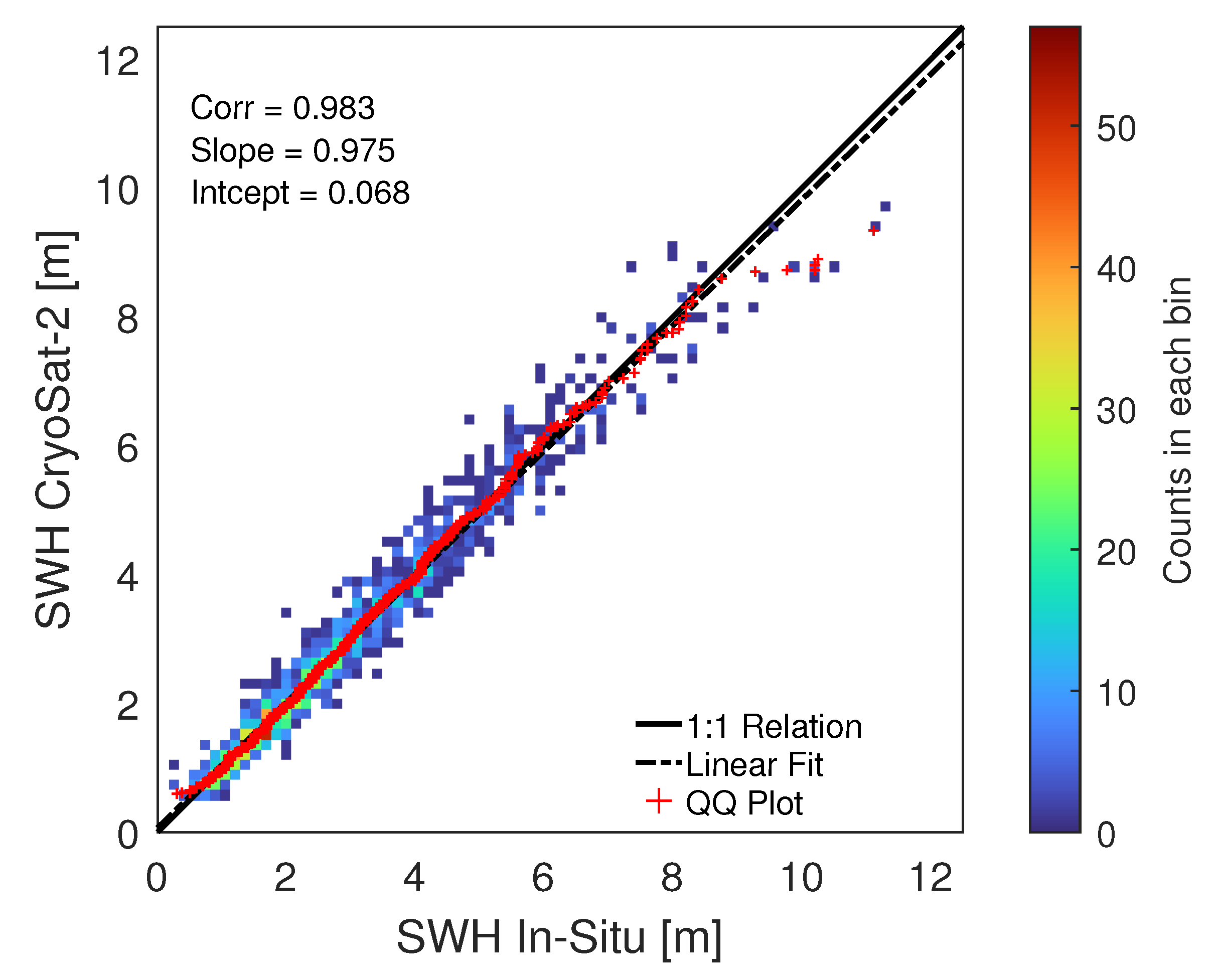
2.3. In Situ CryoSat-2 Correction
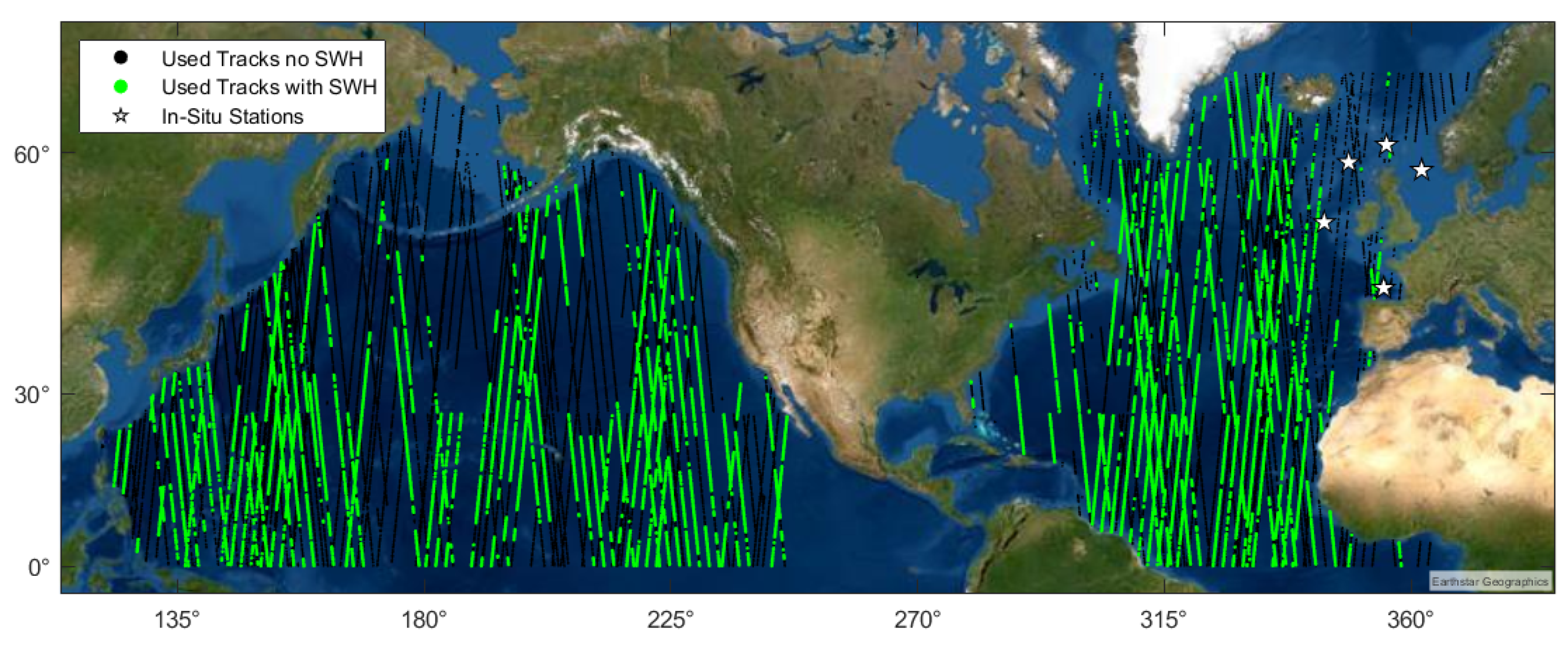
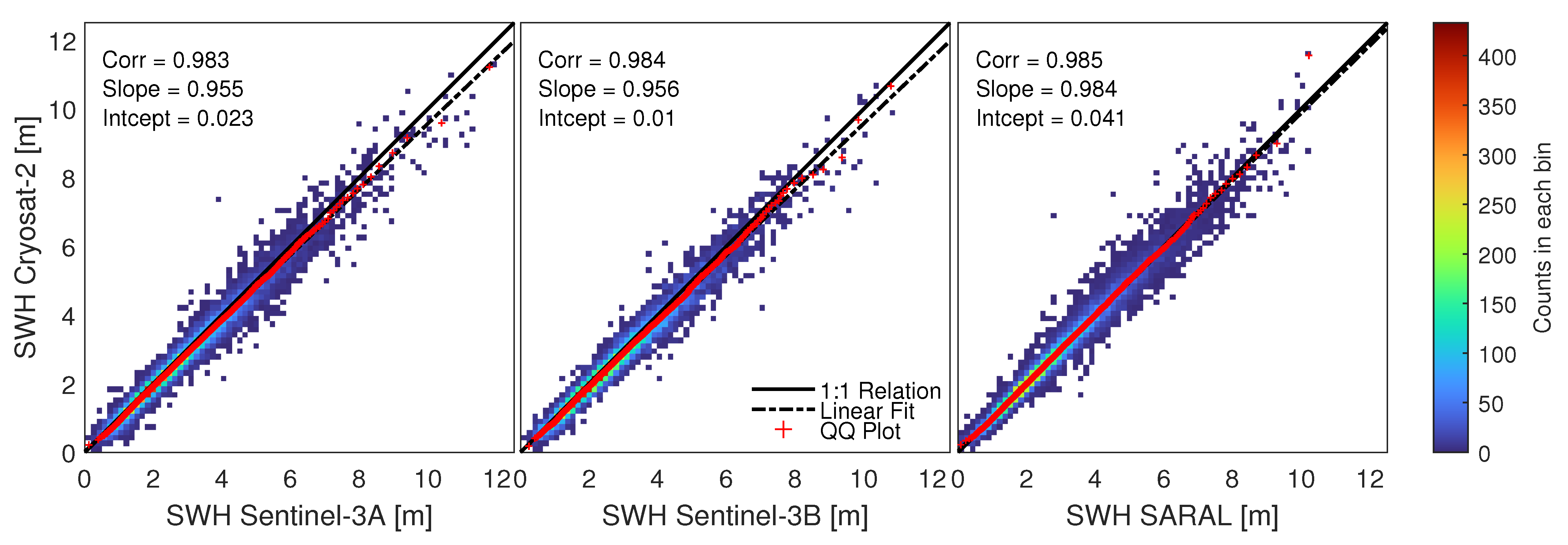
2.4. Satellite Altimeter Crossover Validation
2.5. CRYO2ICE Orbit Matching
3. Methods
3.1. CryoSat-2
3.2. ATL12 SWH
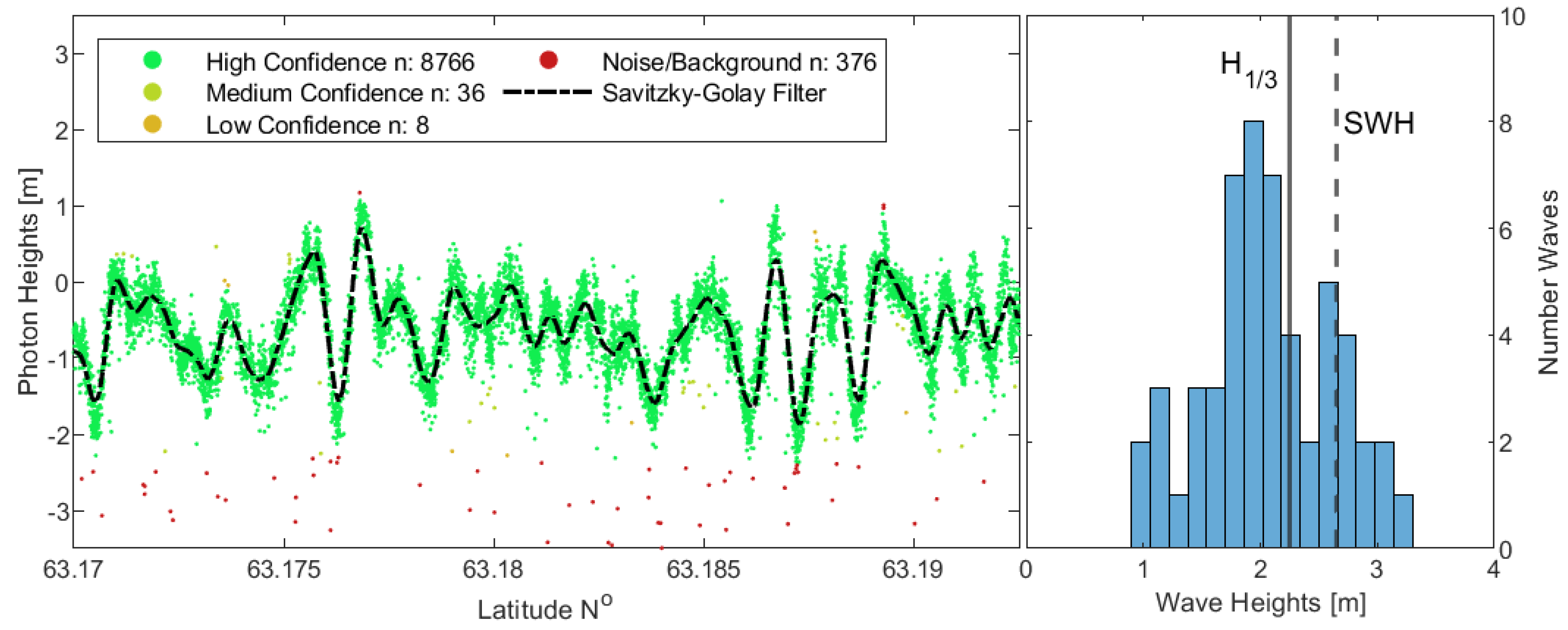
3.3. ATL03
3.3.1. Histogram Model
3.3.2. Standard Deviation Model
4. Results
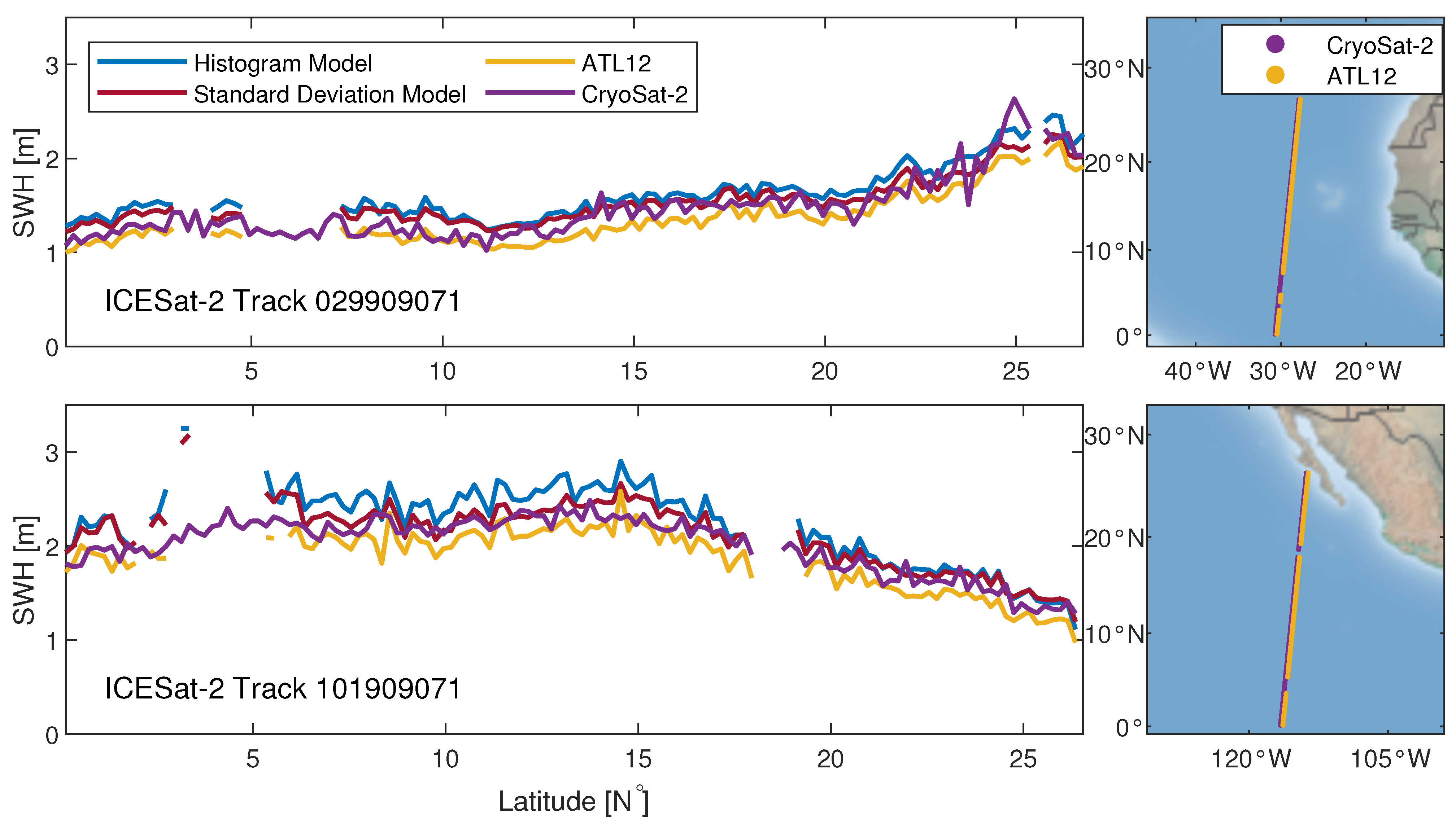
4.1. Orbit Pairing Segmentation
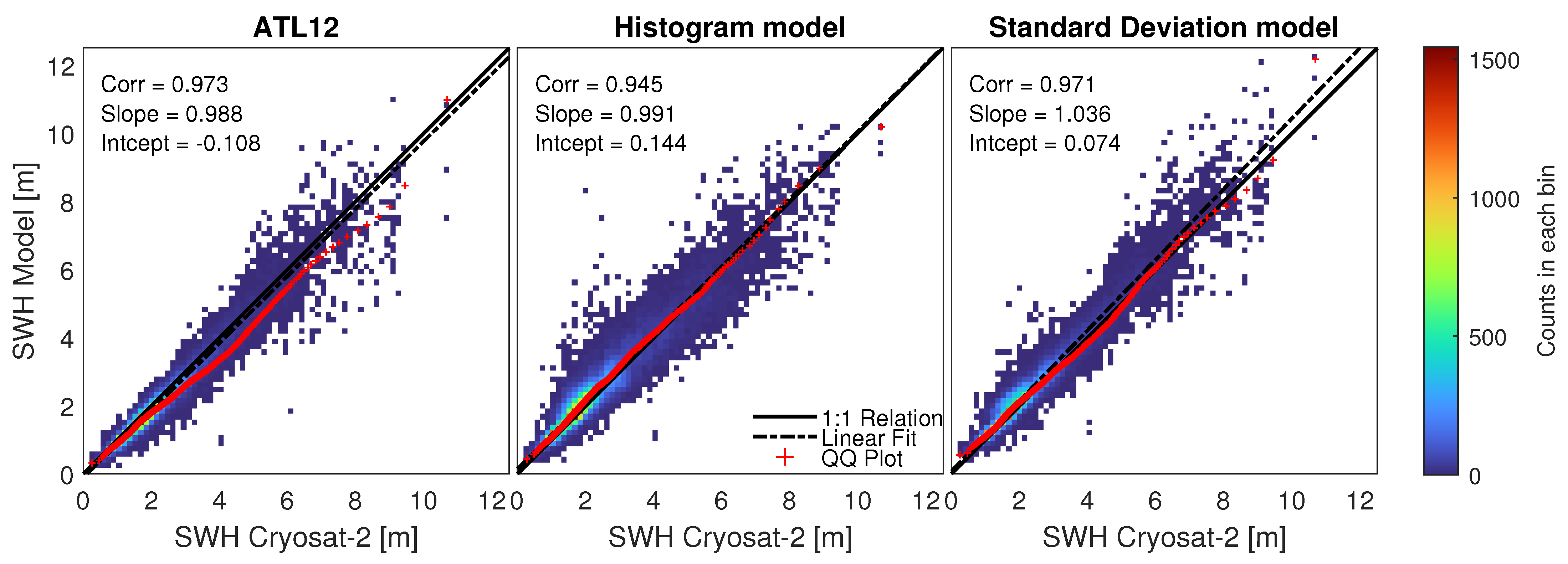
4.2. Full Data Comparisons
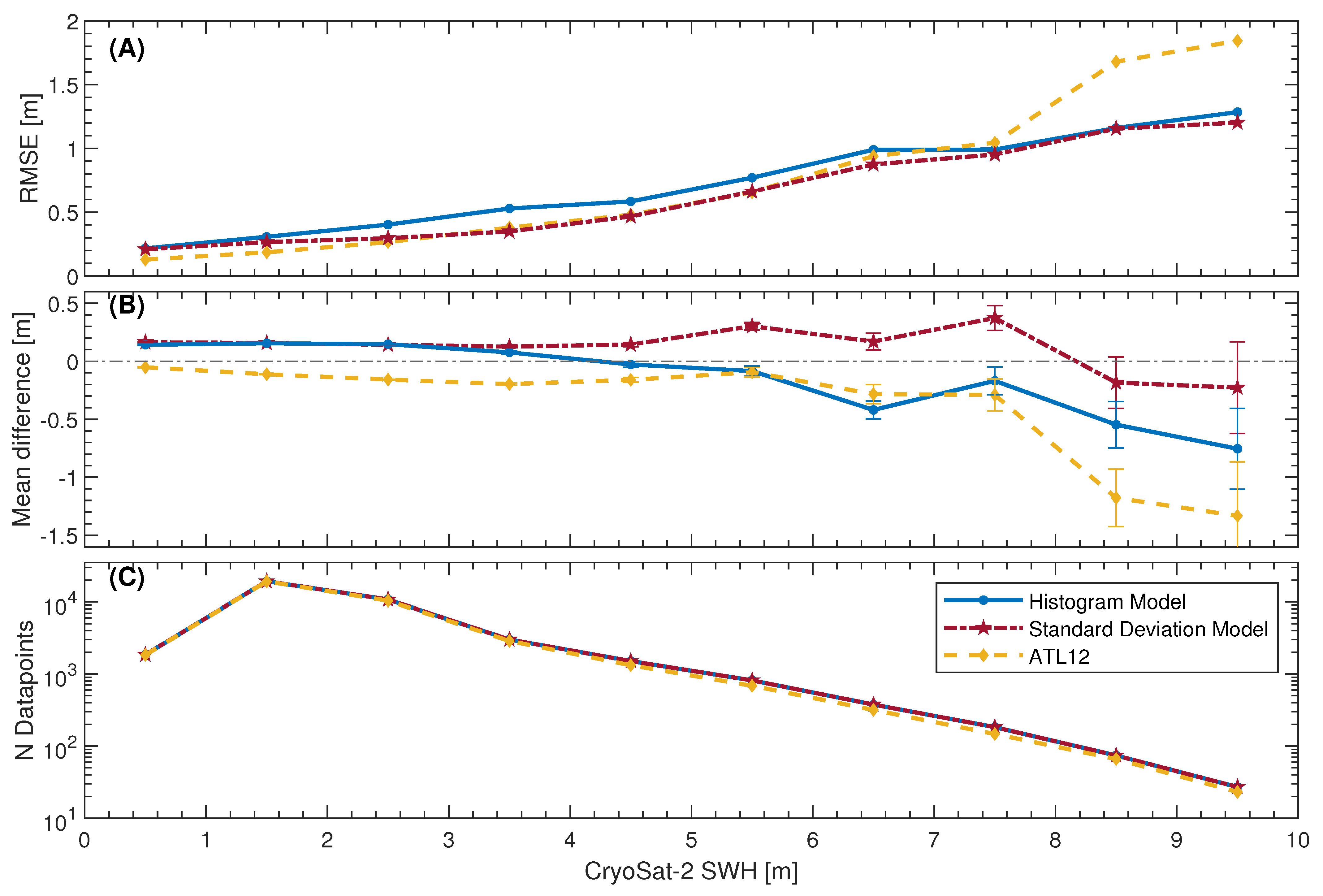
4.3. Sea State Dependency Bias
5. Discussion
6. Conclusions
Author Contributions
Funding
Institutional Review Board Statement
Informed Consent Statement
Data Availability Statement
Acknowledgments
Conflicts of Interest
Abbreviations
| ATLAS | Advanced Topographic Laser Altimeter System |
| ATL03 | ATLAS Global Geolocated Photon Data |
| ATL12 | ATLAS Ocean Surface Height |
| CDF | Cumulative distribution function |
| Variance of surface heights | |
| NOAA | National Oceanic and Atmospheric Administration |
| NSIDC | National Snow and Ice Data Center |
| Probability density function | |
| RADS | Radar Altimeter Database System |
| RMSE | Root mean squared error |
| SAR | Synthetic aperture radar |
| SD | Standard deviation |
| SI | Scatter index |
| SIRAL | SAR Interferometric Radar Altimeter |
| SWH | Significant wave height |
Appendix A. In Situ Stations

| Station Name | Location [lon E/lat N] | Region | Depth [m] |
|---|---|---|---|
| 6200001 | −5.00/45.20 | Bay of Biscay | 4607 |
| 6200095 | −15.86/52.02 | North Atlantic | 3295 |
| 6400045 | −11.40/59.10 | North Atlantic | 2014 |
| 6400046 | −4.50/60.70 | North Atlantic | 1100 |
| Sleipner-A | 1.91/58.37 | North Sea | 96 |
References
- Young, I.R. Wind Generated Ocean Waves; Elsevier: Amsterdam, The Netherlands, 1999; Volume 2, pp. 1–2, 25–27. [Google Scholar]
- Zieger, S.; Vinoth, J.; Young, I.R. Joint calibration of multiplatform altimeter measurements of wind speed and wave height over the past 20 years. J. Atmos. Ocean. Technol. 2009, 26, 2549–2564. [Google Scholar] [CrossRef]
- Klotz, B.W.; Neuenschwander, A.; Magruder, L.A. High-resolution ocean wave and wind characteristics determined by the ICESat-2 land surface algorithm. Geophys. Res. Lett. 2020, 47, e2019GL085907. [Google Scholar] [CrossRef]
- Chelton, D.B.; Ries, J.C.; Haines, B.J.; Fu, L.L.; Callahan, P.S. Satellite Altimetry and Earth Sciences; Academic Press: Cambridge, MA, USA, 2001; Volume 69, pp. 1–131. [Google Scholar]
- Vignudelli, S.; Kostianoy, A.G.; Cipollini, P.; Benveniste, J. Coastal Altimetry; Springer Science & Business Media: Berlin/Heidelberg, Germany, 2011; pp. 1–8. [Google Scholar]
- European Space Agency. CryoSat-2 Product Handbook. Available online: https://earth.esa.int/documents/10174/125272/CryoSat-Baseline-D-Product-Handbook (accessed on 15 August 2021).
- Markus, T.; Neumann, T.; Martino, A.; Abdalati, W.; Brunt, K.; Csatho, B.; Farrell, S.; Fricker, H.; Gardner, A.; Harding, D.; et al. The Ice, Cloud, and land Elevation Satellite-2 (ICESat-2): Science requirements, concept, and implementation. Remote Sens. Environ. 2017, 190, 260–273. [Google Scholar] [CrossRef]
- Morison, J.H.; Hancock, D.; Dickinson, S.; Robbins, J.; Roberts, L.; Kwok, R.; Palm, S.P.; Smith, B.; Jasinski, M.F.; ICESat-2 Science Team. ATLAS/ICESat-2 L3A Ocean Surface Height, Version 4; NASA National Snow and Ice Data Center Distributed Active Archive Center: Boulder, CO, USA, 2021. [CrossRef]
- Kwok, R.; Markus, T. Potential basin-scale estimates of Arctic snow depth with sea ice freeboards from CryoSat-2 and ICESat-2: An exploratory analysis. Adv. Space Res. 2018, 62, 1243–1250. [Google Scholar] [CrossRef]
- Kwok, R.; Kacimi, S.; Webster, M.A.; Kurtz, N.T.; Petty, A.A. Arctic snow depth and sea ice thickness from ICESat-2 and CryoSat-2 freeboards: A first examination. J. Geophys. Res. Ocean. 2020, 125, e2019JC016008. [Google Scholar] [CrossRef]
- Marsh, J.; Webb, E.; Cryosat QC Team. CryoSat CRYO2ICE Orbit Raising Campaign QA4EO QC Summary. Available online: https://earth.esa.int/eogateway/documents/20142/37627/CRYO2ICE-Orbit-Raising-Summary.pdf (accessed on 3 August 2021).
- Sanchez, J.; Marc, X.; Clerigo, I.; Badessi, S.; Bouffard, J.; Hoyos, B.; Casal, T.; Andreoli, F.; Fornarelli, D.; Albini, G.; et al. Introduction to CryoSat-2 ICESat-2 Resonant Orbits. Available online: https://earth.esa.int/eogateway/documents/20142/37627/Introduction-CryoSat-2-ICESat-2-Resonant-Orbits.pdf (accessed on 15 July 2021).
- Bagnardi, M.; Kurtz, N.T.; Petty, A.A.; Kwok, R. Sea surface height anomalies of the Arctic Ocean from ICESat-2: A first examination and comparisons with CryoSat-2. Geophys. Res. Lett. 2021, 48, e2021GL093155. [Google Scholar] [CrossRef]
- Neumann, T.A.; Brenner, A.; Hancock, D.; Robbins, J.; Saba, J.; Harbeck, K.; Gibbons, A.; Lee, J.; Luthcke, S.B.; Rebold, T.; et al. ATLAS/ICESat-2 L2A Global Geolocated Photon Data, Version 4; NASA National Snow and Ice Data Center Distributed Active Archive Center: Boulder, CO, USA, 2021. [CrossRef]
- Morison, J.; Hancock, D.; Dickinson, S.; Robbins, J.; Roberts, L.; Kwok, R.; Palm, S.; Smith, B.; Jasinski, M.; Plant, B.; et al. Algorithm Theoretical Basis Document (ATBD) for Ocean Surface Height Version 4. Available online: https://nsidc.org/sites/nsidc.org/files/technical-references/ICESat2_ATL12_ATBD_r004.pdf (accessed on 26 August 2021).
- Morison, J.; Dickinson, S.; Hancock, D.; Roberts, L.; Robbins, J. Ice, Cloud, and Land Elevation Satellite-2 (ICESat-2) ATL12 Ocean Surface Height Release 004 Application Notes and Known Issues. Available online: https://nsidc.org/sites/nsidc.org/files/technical-references/ICESat2_ATL12_Known_Issues_v004.pdf (accessed on 26 August 2021).
- Scharroo, R. RADS User Manual. Available online: https://github.com/remkos/rads/raw/master/doc/manuals/rads4_user_manual.pdf (accessed on 26 August 2021).
- Scharroo, R.; Leuliette, E.W.; Lillibridge, J.L.; Byrne, D.; Naeije, M.C.; Mitchum, G.T. RADS: Consistent multi-mission products. In Symposium on 20 Years of Progress in Radar Altimetry; ESA: Venice, Italy, 2012; pp. 5–8. Available online: https://ui.adsabs.harvard.edu/abs/2013ESASP.710E..69S/abstract (accessed on 26 August 2021).
- Scharroo, R.; Smith, W.; Leuliette, E.; Lillibridge, J. The Performance of CryoSat-2 as an Ocean Altimeter. Available online: https://ui.adsabs.harvard.edu/abs/2012AGUFM.C54A..05S (accessed on 18 September 2021).
- Bundesamt Für Seeschiffahrt und Hydrographie. North West Shelf Data Portal. Available online: http://nwsportal.bsh.de/ (accessed on 15 May 2021).
- Alford, J.; Ewart, M.; Bizon, J.; Easthope, R.; Gourmelen, N.; Parrinello, T.; Bouffard, J.; Michael, C.; Meloni, M. #CRYO2ICE Coincident Data Explorer, Version 1. Available online: http://cryo2ice.org (accessed on 10 August 2021).
- Casas Prat, M. Overview of Ocean Wave Statistic. Available online: https://upcommons.upc.edu/handle/2099.1/6034 (accessed on 15 August 2021).
- Ranndal, H.; Christiansen, P.S.; Kliving, P.; Andersen, O.B.; Nielsen, K. Evaluation of a statistical approach for extracting shallow water bathymetry signals from ICESat-2 ATL03 photon data. Remote Sens. 2021, 13, 3548. [Google Scholar] [CrossRef]
- Scharroo, R. RADS Data Manual. Available online: https://github.com/remkos/rads/raw/master/doc/manuals/rads4_data_manual.pdf (accessed on 26 August 2021).
| Time Sep. [H] | Sentinel-3A | Sentinel-3B | SARAL | |||||||||
|---|---|---|---|---|---|---|---|---|---|---|---|---|
| Diff. [m] | RMSE [m] | Corr | N | Diff. [m] | RMSE [m] | Corr | N | Diff. [m] | RMSE [m] | Corr | N | |
| 0–1 | 0.106 | 0.188 | 0.995 | 11,466 | 0.117 | 0.198 | 0.995 | 7237 | 0.003 | 0.130 | 0.996 | 16,512 |
| 1–2 | 0.086 | 0.232 | 0.990 | 13,834 | 0.100 | 0.239 | 0.990 | 8664 | 0.002 | 0.178 | 0.993 | 19,259 |
| 2–3 | 0.105 | 0.292 | 0.983 | 11,358 | 0.116 | 0.294 | 0.984 | 6602 | 0.003 | 0.254 | 0.985 | 16,140 |
| 0–3 | 0.092 | 0.308 | 0.981 | 66,253 | 0.100 | 0.308 | 0.981 | 39,711 | 0.002 | 0.269 | 0.983 | 90,500 |
| Data interval: | 1 March 2016 to 24 January 2022 | 8 May 2018 to 25 January 2022 | 14 March 2013 to 26 January 2022 | |||||||||
| CryoSat-2 | ATL12 | Histogram Model | Standard Deviation Model | |
|---|---|---|---|---|
| 5% | 1.01 m | 0.89 m | 1.07 m | 1.11 m |
| 50% | 1.96 m | 1.76 m | 2.06 m | 2.07 m |
| 95% | 4.96 m | 4.32 m | 4.70 m | 4.82 m |
| Max. | 10.68 m | 10.98 m | 10.19 m | 12.17 m |
| SWH | 0–1.5 m | 1.5–2.5 m | 2.5–11 m | |||||||||
|---|---|---|---|---|---|---|---|---|---|---|---|---|
| Models | Diff. | SD | SI | N | Diff. | SD | SI | N | Diff | SD | SI | N |
| Histogram | 0.18 m | 0.23 m | 39.5% | 9883 | 0.18 m | 0.31 m | 17.7% | 18,390 | 0.01 m | 0.59 m | 8.75% | 9583 |
| Standard Deviation | 0.19 m | 0.19 m | 35.7% | 9883 | 0.17 m | 0.23 m | 14.5% | 18,390 | 0.13 m | 0.43 m | 6.67% | 9583 |
| ATL12 | −0.06 m | 0.14 m | 19.77% | 9750 | −0.11 m | 0.17 m | 10.2% | 18,225 | −0.22 m | 0.45 m | 7.36% | 8788 |
| Method | Reference | Mean Diff. [m] | RMSE [m] | Corr. | N |
|---|---|---|---|---|---|
| Validation | |||||
| CryoSat-2 | In Situ | −0.01 | 0.31 | 0.98 | 2124 |
| CryoSat-2 | Sentinel-3A | 0.11 | 0.29 | 0.98 | 11,358 |
| CryoSat-2 | Sentinel-3B | 0.12 | 0.29 | 0.98 | 6602 |
| CryoSat-2 | SARAL | 0.00 | 0.25 | 0.96 | 16,140 |
| Method Comparison | |||||
| Histogram Model | CryoSat-2 | 0.14 | 0.42 | 0.95 | 37,861 |
| Standard Deviation Model | CryoSat-2 | 0.17 | 0.33 | 0.97 | 37,861 |
| ATL12 | CryoSat-2 | −0.12 | 0.29 | 0.97 | 36,763 |
| Analysis by [3] | |||||
| ATL08-Ocean | ERA-5 | 0.07 | 0.38 | 0.91 | N/A |
| ATL12 | ERA-5 | −0.16 | 0.33 | 0.95 | N/A |
| CryoSat-2 | ERA-5 | −0.01 | 0.36 | 0.95 | N/A |
Publisher’s Note: MDPI stays neutral with regard to jurisdictional claims in published maps and institutional affiliations. |
© 2022 by the authors. Licensee MDPI, Basel, Switzerland. This article is an open access article distributed under the terms and conditions of the Creative Commons Attribution (CC BY) license (https://creativecommons.org/licenses/by/4.0/).
Share and Cite
Nilsson, B.; Andersen, O.B.; Ranndal, H.; Rasmussen, M.L. Consolidating ICESat-2 Ocean Wave Characteristics with CryoSat-2 during the CRYO2ICE Campaign. Remote Sens. 2022, 14, 1300. https://doi.org/10.3390/rs14061300
Nilsson B, Andersen OB, Ranndal H, Rasmussen ML. Consolidating ICESat-2 Ocean Wave Characteristics with CryoSat-2 during the CRYO2ICE Campaign. Remote Sensing. 2022; 14(6):1300. https://doi.org/10.3390/rs14061300
Chicago/Turabian StyleNilsson, Bjarke, Ole Baltazar Andersen, Heidi Ranndal, and Mikkel Lydholm Rasmussen. 2022. "Consolidating ICESat-2 Ocean Wave Characteristics with CryoSat-2 during the CRYO2ICE Campaign" Remote Sensing 14, no. 6: 1300. https://doi.org/10.3390/rs14061300
APA StyleNilsson, B., Andersen, O. B., Ranndal, H., & Rasmussen, M. L. (2022). Consolidating ICESat-2 Ocean Wave Characteristics with CryoSat-2 during the CRYO2ICE Campaign. Remote Sensing, 14(6), 1300. https://doi.org/10.3390/rs14061300