Article

Voids Filling of DEM with Multiattention Generative Adversarial Network Model

1
Guangxi Key Laboratory of Spatial Information and Geomatics, Guilin University of Technology, Guilin 541004, China
2
College of Geomatics and Geoinformation, Guilin University of Technology, Guilin 541004, China
3
College of Earth Sciences, Guilin University of Technology, Guilin 541004, China
*
Author to whom correspondence should be addressed.
Remote Sens. 2022, 14(5), 1206; https://doi.org/10.3390/rs14051206
Submission received: 21 January 2022 / Revised: 17 February 2022 / Accepted: 25 February 2022 / Published: 1 March 2022

Abstract

:
The digital elevation model (DEM) acquired through photogrammetry or LiDAR usually exposes voids due to phenomena such as instrumentation artifact, ground occlusion, etc. For this reason, this paper proposes a multiattention generative adversarial network model to fill the voids. In this model, a multiscale feature fusion generation network is proposed to initially fill the voids, and then a multiattention filling network is proposed to recover the detailed features of the terrain surrounding the void area, and the channel-spatial cropping attention mechanism module is proposed as an enhancement of the network. Spectral normalization is added to each convolution layer in the discriminator network. Finally, the training of the model by a combined loss function, including reconstruction loss and adversarial loss, is optimized. Three groups of experiments with four different types of terrains, hillsides, valleys, ridges and hills, are conducted for validation of the proposed model. The experimental results show that (1) the structural similarity surrounding terrestrial voids in the three types of terrains (i.e., hillside, valley, and ridge) can reach 80–90%, which implies that the DEM accuracy can be improved by at least 10% relative to the traditional interpolation methods (i.e., Kriging, IDW, and Spline), and can reach 57.4%, while other deep learning models (i.e., CE, GL and CR) only reach 43.2%, 17.1% and 11.4% in the hilly areas, respectively. Therefore, it can be concluded that the structural similarity surrounding the terrestrial voids filled using the model proposed in this paper can reach 60–90% upon the types of terrain, such as hillside, valley, ridge, and hill.

1. Introduction

The digital elevation model (DEM) is one of the sources of national geospatial infrastructure [1,2] and has been widely used in many fields, such as topographic mapping [3,4], ocean monitoring [5,6], glacial evolution detection [7], smart cities [8], and global land change [9]. The quality of a DEM is a basis for the applications and is checked during every step of producing the DEM, from the collection of elevations to the interpolation implemented for resampling [10]. For example, it is unavoidable for a DEM to result in voids due to ground occlusion, among others, resulting in a significantly low-quality spatial analysis relevant to terrain [11,12,13]. Therefore, filling a DEM void is critical for both DEM quality and its applications [14,15].
Many researchers have studied the different algorithms for DEM void filling. In the early work, the traditional interpolation methods, such as inverse distance weighted interpolation (IDW) [16] and Kriging [17], have been widely used. These methods are effective in flat and low-lying terrestrial areas, but are easily impacted by topographical undulations [18]. For this reason, some scholars introduced the concept of image processing to fill the DEM voids. The method, called filling and feathering (FF), is popular and also effective; it uses the feathering process to smooth the sudden changes of the edge. Especially when size of the DEM void is small, this method can obtain a very satisfactory result. Grohman et al. proposed a delta surface fill (DSF) method [18], which is an improvement of FF methods, using auxiliary data to fill voids and get smoother data without feathering. Luedeling et al. [19] improved the DSF method and proposed a more promising method based on a triangular irregular network (TIN), which can better deal with the elevation deviation between different data. In addition, Spline and the advanced Spline method (ANUDEM) [20,21,22] have also been applied to the more specific task of filling DEM voids. On the other hand, a few scholars suggest adding some topographic features as auxiliary data for DEM void filling on the basis of the interpolation method, such as [17,23,24]. Ling et al. [25] are one of the first people who proposed to fill voids on the basis of the trend of valleys in satellite images. Hogan et al. [26] proposed using geometric shadow constraints to fill voids. However, the shadow itself is relatively sparse information, resulting in relatively low accuracy. Yue et al. [27] constructed a high-accuracy surface model (HASM) using the basic geometric feature constraints of landmarks and auxiliary data to fill voids. Soon after, Yue et al. [28] applied HASM to fill voids on the XCO2 surface of GOSAT and SCIAMACHY and achieved good results. Yue et al. [29] used ASTER GDEM v2 and ICTESat to fill the SRTM-1 data voids encountered in the original data to generate a high accuracy and high quality of DEM. Although the methods using interpolation techniques can fill DEM voids well, it heavily relies on the DEM’s local features, such as void size, terrestrial slopes, etc. [30].
In recent years, with the rapid development of deep learning (DL), the DL method has been widely applied in many fields, for instance, image repair [31,32,33]. Therefore, many scholars consider the DEM void filling as image repair, and further use the DL to resolve the limitations of interpolation methods. For example, Goodfellow et al. [34] succeeded in generating images with reasonably clear semantic structure by adversarial training of generators and discriminators. Iizuka et al. [35] proposed a network model with dual discriminators based on generative adversarial networks, and the dual discriminator structure can ensure the global-local consistency of image filling while enhancing the stability of training. Liu et al. [36] introduced partial convolution into the model, and the key idea of partial convolution is to divide the feature image into valid and invalid parts, thus improving the accuracy of filling voids. Dong et al. [30] developed a conditional adversarial network (CAN) framework that employs an L1 norm to constrain the CAN training process for filling shuttle radar topography mission (SRTM) void data. Qiu et al. [37] proposed a terrain texture generation network model, which generated a satisfactory fill surface by constructing samples composed of elevation, terrain slope, and relief degree and designing a loss function composed of pixel-wise, contextual and perceptual loss. However, the TTGM also requires a post-processing step that uses Poisson blur to fuse the resulting filled surface with the original data. Dong et al. [38] used terrain shading as a constraint for conditional generation adversarial networks for filling DEM voids. However, this method has high time and labor costs due to use the filling of data based on field surveys and in situ measurements to train the model. Hui et al. [39] proposed a dense multiscale fusion block for expanding the convolutional kernel receptive field and ensuring the denseness of the convolutional kernels, which have a good result.
On the other hand, Jaderberg et al. [40] first proposed a parameter spatial attention model (Spatial Transformer Network, STN) for target classification tasks. Afterward, many scholars have added the attention mechanism module to the network model. Hu et al. [41] proposed enhancing the ability of the model for the extraction of key features to obtain a high accuracy of filling results. Yu et al. [42] proposed a contextual attention mechanism that processes the feature graph in the deep space of the network. It can extract important features in known regions to fill voids. Wang et al. [43] proposed a multiscale attention mechanism, which is a model that can flexibly process background useful information and suppress useless information. Gavriil et al. [44] proposed a Wasserstein generative adversarial network (WGAN) network structure based on the contextual attention mechanism to fill the DEM holes. Zhang et al. [45] proposed a deep generation model (DGM) in which the reconstruction loss and generative adversarial network (GAN) loss are used to assist network training, and combination with the contextual attention layer to fill the void areas. Zhu et al. [46] designed conditional encoder–decoder generative adversarial neural networks (CEDGANs) to fill the voids, which combines the encoder–decoder structure with adversarial learning to get deep representations of sampled spatial data and the interaction of local structural patterns. Li et al. [47] proposed a topographic knowledge-constrained conditional generative adversarial network (TKCGAN) to fill the voids, which uses qualitative topographic knowledge of valleys and ridges to transform new loss functions. The filling result by WGAN has high accuracy and conforms to topographical fluctuations, but requires additional boundary smoothing processing. Although the methods based on attention mechanisms can extract key information in feature maps, most of them have not considered the internal relationship between features, especially global and local features.
With the reviews above, it can be summarized that the problems of filling DEM voids consist of: (1) the existing models cannot achieve high accuracy for the filled DEM voids in complex terrain, i.e., inconsistent similarity structure surrounding the DEM void area; (2) ignoring how the other features surrounding the DEM void in spatial dimension impact the accuracy of the filled DEM void. For this reason, a multiattention generative adversarial networks model for filling DEM voids is proposed in this paper.

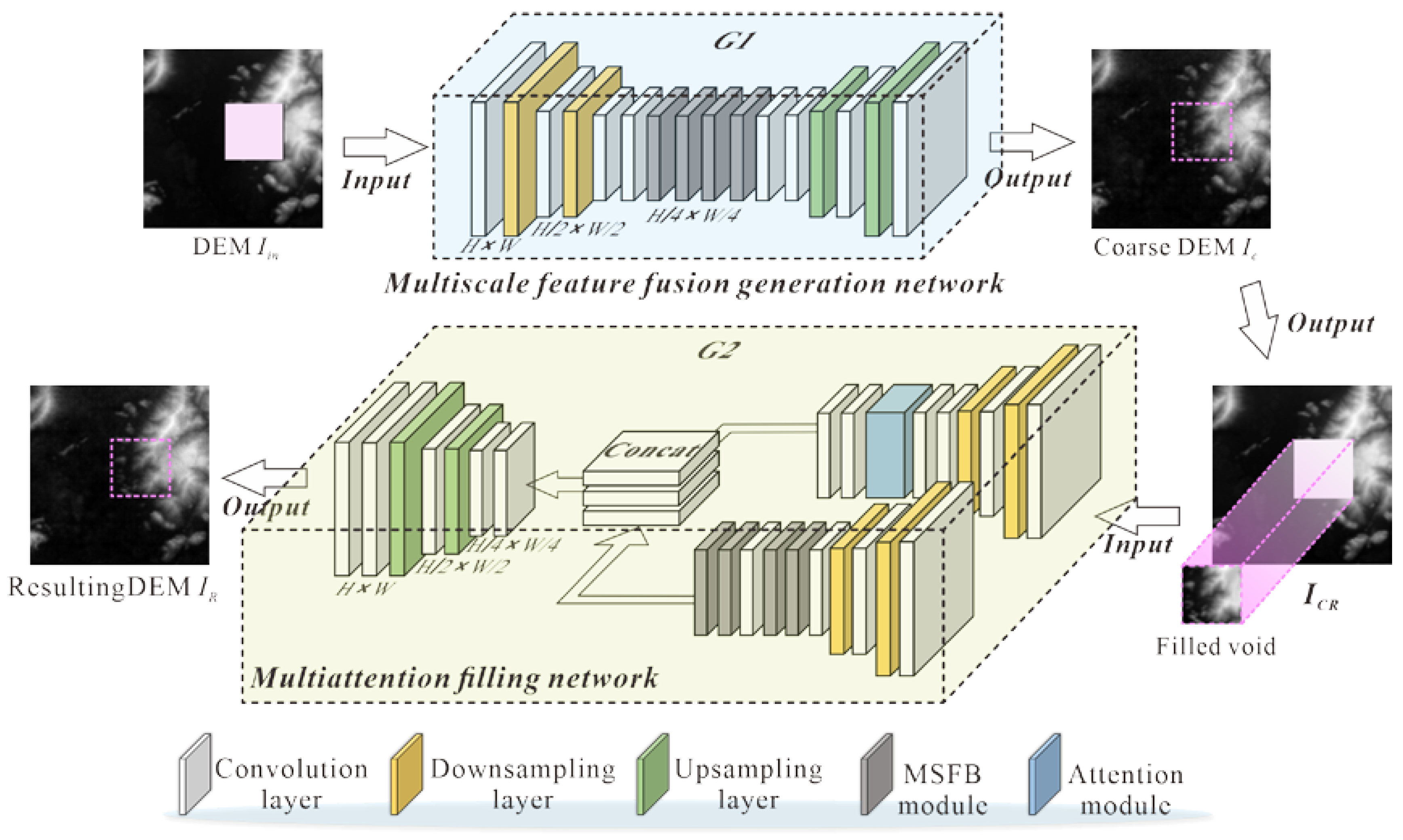
2. A Multiattention Generative Adversarial Network Filling Model

The model architecture proposed in this paper is shown in Figure 1. DEM data Iin, which have voids, are first input into a multiscale feature fusion generation network, and the extracted deep features are then reconstructed to approximate the distribution pattern of the original data Iin. The part of the missing area in IC is added to the missing data Iin, and an initial filling result ICR is output. Then, the model takes the ICR input to the multiattention filling network. After a series of convolution and deconvolution operations, it obtains a more refined result with detailed texture. Finally, the reconstruction loss and the adversarial loss are calculated separately. The global-local adversarial network is optimally trained to obtain a high-precision deep network filling model. The detail for the proposed model is given as follows.

2.1. Multiscale Feature Fusion Generation Network

2.1.1. Network Structure Design

The multiscale feature fusion generation network utilizes the basic VGG16 network structure, as shown in G1 of Figure 1. The G1 module takes the original image Iin and the binary mask M as input. The size of the input original image is H × W × C, where H represents the image height, W is the image width, and C is the number of channels of the image. The binary mask matrix has a value of 0 or 1 (where 0 is for the known area and 1 for the void area) and a size of H × W × 1. The missing image is simulated by the original image multiplying the binary mask matrix. The missing image first passes through six convolution layers with a filter size of 3 × 3 pixels2, and each convolutional layer is followed by a batch normalization (BN) layer. In particular, the ReLU function is used for all layers except for the last layer of the output network, where the tanh function is used for the activation function. In this stage, the convolutional layer instead of the maximum pooling layer is used for downsampling and only downsamples the image twice, with a final feature map size of (H/4 × W/4 × 256). Then, the multiscale feature fusion module (MSFF) is introduced, which is described in detail in the following subsections.
The MSFF module can expand the receptive field of the convolution kernel to further extract information from the feature map obtained in the previous step and obtain the feature map with the same size of (H/4 × W/4 × 256). Finally, the feature maps are passed through six deconvolution layers with a filter size of 3 × 3 pixels2. This reconstructs the feature distribution of the original image by upsampling twice and outputs a fake image IC with the same size as the original image Iin. Using the following equation for calculation, the initial repaired image ICR with a size of H × W × C is obtained, i.e.,
I C R = I i n ( 1 M ) + I C M

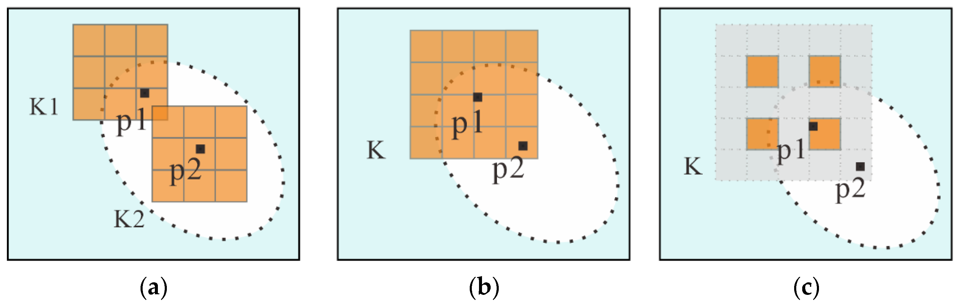
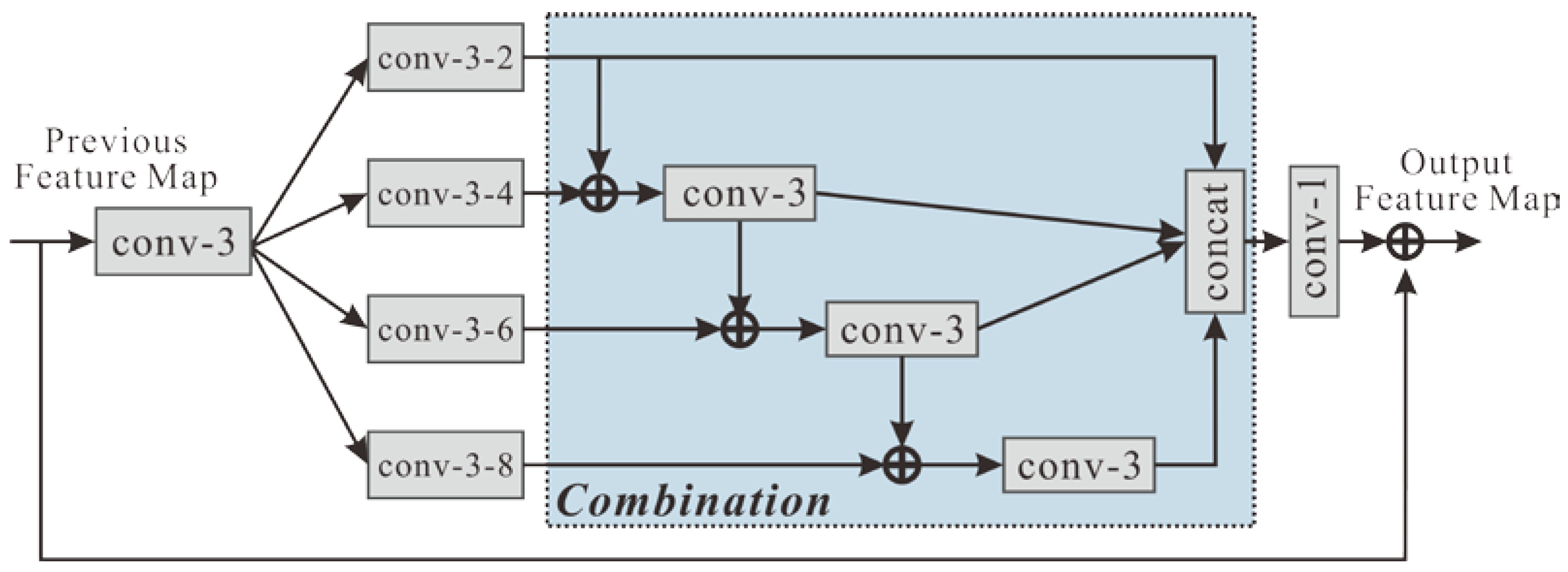
2.1.2. Multiscale Feature Fusion Module

In order to achieve the fill of large void areas, the output pixels within the voids must contain spatial support for the pixels in the known area, as shown in Figure 2. The receptive field is the size of the area where each pixel of the feature map is affected by the convolution of the previous feature map. The larger receptive field means that more comprehensive information of the feature map can be obtained [34]. To this end, Yu et al. [42] used a 7 × 7 pixels2-sized convolutional kernel for feature extraction to achieve an expanded field of perception, but this adds additional parameters. Dilated convolution was first proposed as a convolution idea for image semantic segmentation tasks where downsampling would degrade image resolution and lose information. Many researchers have started to solve this problem using dilated convolution and achieved promising performance [34,48]. However, since the dilated convolution is sparse, many pixels are ignored in performing feature extraction [49]. For this reason, this paper applies the multiscale feature fusion module to the network model [50], as shown in Figure 3. The MSFF module first decreases the number of channels of the feature map x0 by the first convolution layer, thus reducing the number of model parameters. Then, each of the four branches of the dilated convolution (rate = 2, 4, 6 and 8) is processed. The feature maps x1, x2, x3 and x4 in the combined computation, except for x1, are obtained, which is allowed to be output directly to the last layer. The rest of the feature map xi needs to be downsampled by a convolution kernel of size 3 × 3 pixels2. Then, after a series of overlay combination operations, the sparse feature map xi is used to combine the dense multiscale feature maps. Finally, the dense multiscale feature maps are convolved once and then combined with x0. The formula for the combination calculation is by
y i = { x i , i = 1 ; K i ( x i 1 + x i ) , i = 2 ; K i ( y i 1 + x i ) i = 3 , 4 ;
where xi is the feature map output from the convolution layer. Ki is the kernel of one of the convolution layers. yi is the feature map after the overlay combination.

2.2. Multiattention Filling Network

After obtaining the initially filled results using the G1 network, it is necessary to implement the fill of data detail features. The multiattention filling network is proposed to achieve this purpose. Unlike the G1 network, the G2 module is divided into the regular branch and the attention branch. More detailed description is provided below.

2.2.1. Network Structure Designs

The multiattention filling network also adopts the basic network structure of VGG16, but the channel-spatial pruning attention (CSPA) module is applied in the encoding stage of the G2 model, as shown in G2 of Figure 1.
In the multiattention filling network, the initially filled data ICR are used as the input into the G2 network. The regular branch adopts the same structure as the encoding stage of the G1 network. First, the feature map F1 is obtained after six convolution layers with a filter size of 3 × 3 pixels2. Then, the MSFF module is used to further extract features and obtain the feature map FM. Two downsampling operations are carried out on the ICR by six convolutional layers to obtain the feature map F2 in the attention branch. A multiattention mechanism module is integrated immediately afterward, which is used to capture the local similarities and global dependencies of the feature maps and to output the feature map FS. Finally, FM and FS are merged. Then, after a series of deconvolution operations, the data IR generated by the multiattention filling network are obtained. The final fill result Iinpaint is obtained by the following formula:
I i n p a i n t = I i n ( 1 M ) + I R M

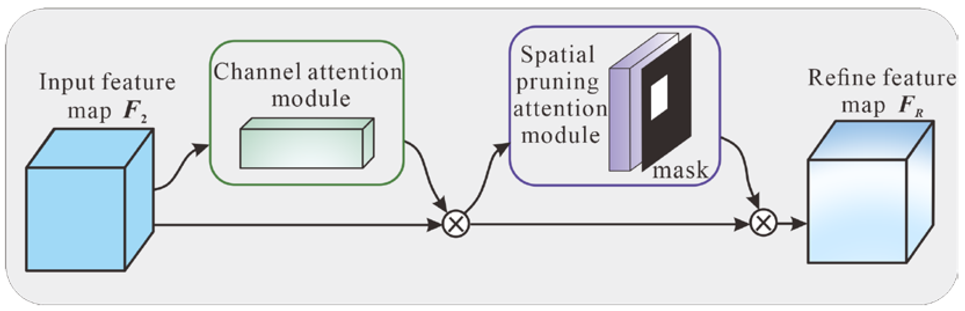
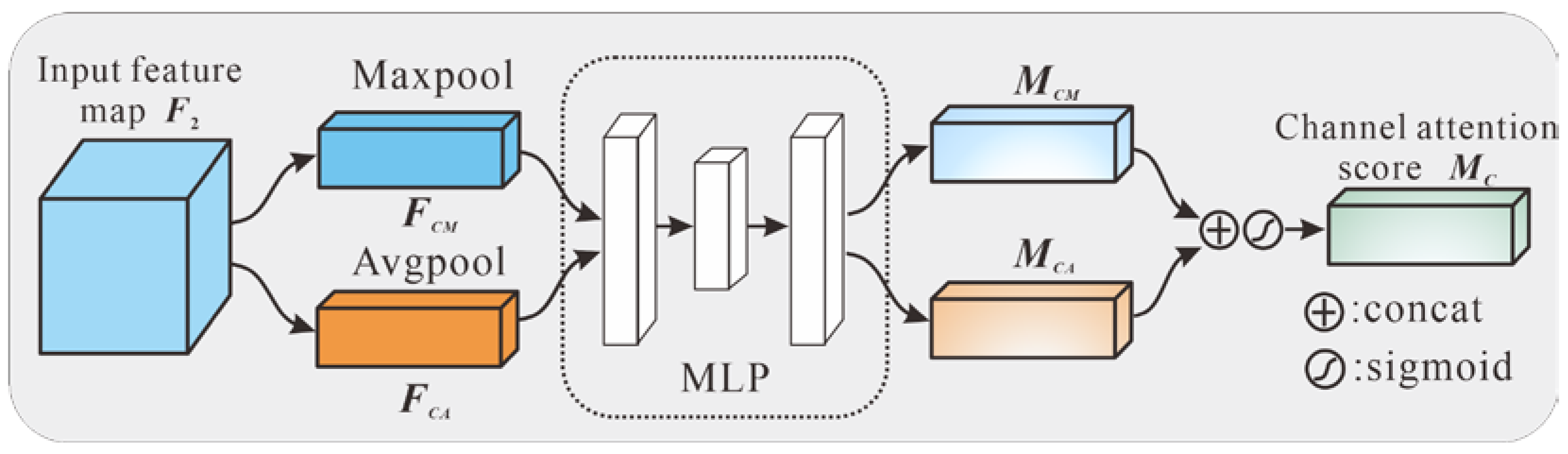
2.2.2. Multiattention Mechanism Module

The multiattention mechanism module takes feature map F2 and mask M as input. First, this module inputs feature map F2 to the channel attention module, which can calculate the attention fraction between each feature map on the channel domain to obtain the channel attention Mc and feature map FC. Then, the FC and mask M are input to the spatial cropping attention module. The attention score MS, which indicates the correlation between the pixels on the feature map, is calculated. The final refined feature map FR is obtained. The overall structure of the module is shown in Figure 4. The detailed structure of the channel attention module is shown in Figure 5, and the detailed structure of the spatial pruning attention module is shown in Figure 6.
The channel attention module takes the feature map F2 as input and downsamples the feature map using maximum pooling and average pooling [17] to obtain the one-dimensional feature maps FCM and FCA. FCM and FCA are input to the three fully connected layers and output MCM and MCA to calculate the dependency between feature maps. Finally, MCM and MCA are combined into the channel dimension, and the channel attention MC is obtained by using the sigmoid activation function. The feature map F2 is matrix multiplied with the channel attention MC to obtain the feature map FC.
The input of the spatial pruning attention module is the feature map FC and mask M. Traditional methods use maximum pooling or average pooling to downsample interchannel feature maps, but this method is too “violent” and can easily cause a large amount of feature information loss [39]. Therefore, the feature map FC is downsampled with four convolutional kernels of different sizes, whose structure is shown in Figure 6.
The spatial pruning attention mechanism obtains the correlation between feature values by matrix multiplication between feature maps. The feature correlation map ρ between the feature maps w1(FC) and w2(FC) is calculated after convolution, which is calculated by
ρ = w 1 ( F c ) T w 2 ( F c )
where w(∙) is a 1 × 1 pixels2 convolution kernel and ⊗ denotes matrix multiplication.
With the calculation above, the pruned feature correlation map ρΜ is obtained by multiplying by the downsampled mask M and the feature correlation map ρ. By pruning, the less relevant feature values are removed and features are only focused on void filling, which is calculated with
ρ M = ρ M
where ⊙ denotes matrix dot multiply.
After obtaining the pruned feature correlation map ρΜ, the global association score Kρ is calculated using the softmax function by
K ρ = exp ( ρ M ) i exp ( ρ M i )
Finally, the feature map w3(FC) is multiplied by the global correlation score Kρ to obtain the spatial attention MS. Then, MS is multiplied by the feature map FC to obtain the final output refined feature map FR.
M s = w 3 ( F c ) K ρ
F R = F c M s

2.3. Global-Local Adversarial Network

The global-local adversarial network, consisting of the two parts of the global discriminator and local discriminator, is shown in Figure 7. By adding a local discriminator to the traditional generative adversarial network, it can constrain whether the filling void area is smooth and coherent with the known region. The inputting data of the global discriminator network are the original data and the data after G2 filling. First, five convolutional layers are used for downsampling, where the size of the convolutional kernel is 5 × 5 pixels2 and the step strides are 2. Notably, a spectral normalization constraint is applied to each convolutional layer [50]. The extracted features are then reshaped into a vector of length 2048 by a fully connected layer. The local discriminator takes the filled data at the void area and the original data of the void area as input. The feature extraction process is similar to that of the global discriminator, which first passes through four convolutional layers for downsampling. The filter size of the convolutional kernel is 4 × 4 pixels2, and the step strides are 2. The extracted features are then reshaped into a vector of length 2048 by a fully connected layer. Finally, the vectors output by the local discriminator and the global discriminator are combined into a vector of length 4096 and input to a fully connected layer. The probability that the output data are true data after the sigmoid activation function needs to be determined. The parameters of the generator and discriminator are updated by computing the gradient of the loss function with the penalty, i.e., the data fill results are discriminated by combining the recognition results of the two discriminators for the data.

2.4. Combined Loss Function

Generally, there is an objective function in the deep learning model. The training process of the network seeks the optimal parameters of a set of networks by solving for the optimal value of the objective function. Unlike other filling models, the Wasserstein distance in WGAN is applied to measure the mapped and original data [51]. In addition, a gradient penalty is added to the adversarial loss of the WGAN. The Wasserstein distance generates a continuously changing gradient to optimize the entire network, and the gradient penalty avoids extremes in the discriminator network parameters. Therefore, the adversarial loss function in this paper can be expressed as:
min   max { E x r p r [ D ( x r ) ] E x g p g [ D ( x g ) ] + α E x p x [ | x D ( x ) | 2 1 ] 2 }
x = ε x r + ( 1 + ε ) x g
where xr is the real data and Pr is the probability density distribution of the original data. xg is the mapped data, and Pg is the probability density distribution of the mapped data. x is a random interpolation sample between xr and xg, and P x is the probability density distribution of x . ε is a random number obeying a uniform distribution on the interval [0,1]. α is the weighting factor of the penalty term.
The adversarial loss function of the generator is:
min E x g p g [ D ( x g ) ]
The adversarial loss function of the discriminator is:
min { E x g p g [ D ( x g ) ] E x r p r [ D ( x r ) ] + α E x p x [ | | x D ( x ) | | 2 1 ] 2 }
In GAN, to make the generated image have the same features as the real image, it is also necessary to consider regularization at the pixel level. Therefore, reconstruction loss is chosen to optimize the generator. The reconstruction loss uses the L1 or L2 norm to constrain the pixel-level information of both to prevent overfitting [48]. Since the model eventually only needs to consider data from the void area, a binary mask is added to indicate the location of the void area.
L p i x = 1 n i = 1 n M | | x r i x g i | | 2
where M is the mask matrix. ⊙ denotes the matrix dot multiplied, and n is the total number of image pixels.
Therefore, the reconstruction loss and the adversarial loss is combined as the model’s objective function, i.e.,
L = λ p i x L p i x + λ a d v L a d v
where L is the objective loss of the model. Lpix is the reconstruction loss, and the L2 norm is used as the measurement distance of the reconstruction loss in this paper. λpix and λadv are their weighting coefficients.

3. Experiment and Analysis

3.1. Experimental Data and Preprocessing

3.1.1. Datasets

The experimental data in this paper were obtained from the ASTER GDEM V2 dataset (https://search.earthdata.nasa.gov/search/, accessed on 26 October 2021), with a data resolution of 30 m. To test the performance of our filling model, DEMs from four regions of China (see Figure 8), namely, Guangxi Province, Guizhou Province, Heilongjiang Province and Xinjiang Province, were selected as training samples, where the types of terrain included hills, plains and valleys. To reduce the training time, the DEMs are cropped to (64 × 64) size. A total of 10,000 DEM images are obtained, of which 9500 are used as the training dataset and 500 are used as the test set. We randomly generate a mask matrix with sizes ranging from (12 × 12) to (32 × 32) during the training process. The original DEM image and mask matrix are then used as input data to simulate the DEM image with holes. We make 5 mask operations on each DEM image during testing to verify the accuracy of the model. We use the mean error, mean absolute error, root mean square error, peak signal-to-noise ratio and structural similarity index as the evaluation indices of accuracy. The experiments include the repair of images with different areas and different hole sizes. In addition, a comparison analysis with other different repair methods is performed.

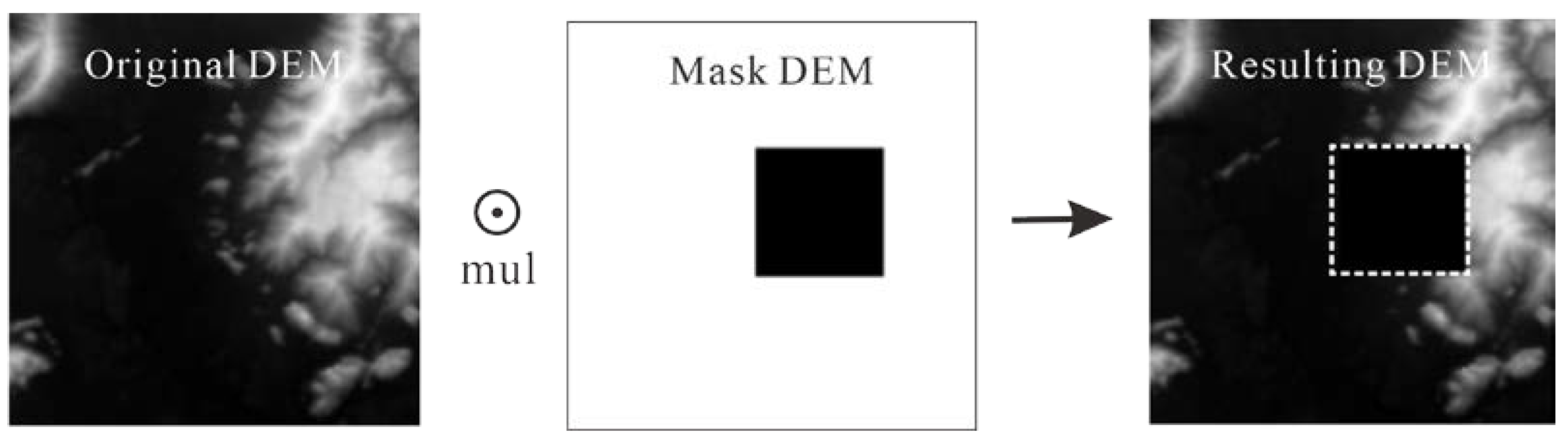
3.1.2. Data Preprocessing

To accelerate the convergence of the calculation and stabilize the network against training, the tailored DEM image training set is normalized to the [0, 1] range by normalizing the elevation values of each image before the training starts. Because the activation function of the final output layer of the model is tanh, the value of the output image is in the range of [−1, 1]. It is also necessary to reduce the value of the normalized image to the [−1, 1].
For the DEM image training set, the randomly generated binary masks are used for matrix multiplication, and for simulating DEM images with voids. The size of the mask matrix is the same as the size of the original image, but the values in the mask matrix include only 0 and 1. The mask matrix is multiplied by the original image pixel by pixel. The location multiplied by 0 is the area to be filled, and the location multiplied by 1 is the known area. As shown in Figure 9, this paper uses the product of the original data and the mask matrix to obtain the data with voids. To smoothly connect the filled area with the known area, local pre-fill is used by expanding the filling area to be filled outward by a few pixels, which can help the model fit the features at the edges of the original void area.
To balance the adversarial training between the discriminator and generator, the model is pre-trained with TC times. The detailed training steps are shown in Table 1.
This experiment adopts the Adam gradient optimization algorithm [52] to optimize the model, which is an adaptation learning rate optimization algorithm. In this experiment, the hyperparameter learning rate of the Adam optimizer is set to 2.0 × 10⁻⁴, and beta1 is the default value. After several experiments, the coefficients of the model combined loss function were set to λpix = 0.99 and λadv = 0.01. The model was trained for a total of T = 2000 epochs, where the number of portraits of the rough generative DEM network was TC = 100 epochs.

3.1.3. Evaluation Metrics

In order to further evaluate the accuracy of filling voids, this paper selects mean error (ME), mean absolute error (MAE), and root mean square error (RMSE) as evaluation indexes, i.e.,
M E = 1 N i N ( y i y i )
M A E = 1 N i N | y i y i |
R M S E = 1 N i N ( y i y i ) 2
where y i and y i represent the elevation value of each pixel of the filling result and the original data, and N is the total number of pixels in the void area of each datum.
In addition, this paper uses peak signal-to-noise ratio (PSNR) [53] and structural similarity (SSIM) [54] for evaluation of the similarity structure of terrain surrounding the void.
P S N R = 10 * l o g 10 ( ( 2 n 1 ) 2 M S E )
where MSE is mean square error.
S S I M ( R , F ) = ( 2 μ R μ F + c 1 ) ( 2 σ R F + c 2 ) ( μ R 2 + μ F 2 + c 1 ) ( σ R 2 + σ F 2 + c 2 )
where R is the original data, F is the result data, μ R is the average gray of R, μ R F is the average gray of F, and σ R F is the covariance of R and F; σ R is the standard deviation of R, σ F is the standard deviation of F, and c1 and c2 are constants with extremely small values, which are used to prevent the denominator from being zero.

3.2. The Filled Results in Four Test Areas

To verify that the proposed filling model can effectively fill the missing areas in the DEM, four representative areas were selected. The types of landforms are located in mountains or valleys. Then, the void area was randomly dug, and the results are shown in Figure 10. The experimental conclusion is as follows.
Area 1 is located in the northwest of Heilongjiang Province, with relatively gentle terrain and simple topography. The maximum height difference is 169 m (the minimum elevation is 326 m, and the maximum elevation is 495 m). As shown in Figure 10(a1), the void area is located at the hill slope, and the void crosses a large area. From the experimental results, the boundary connection between the filling result and the original DEM is rather smooth. In addition, the characteristics of the void area have been recovered. As shown in Table 2, the value of ME is 1.37 m, and the value of RMSE is 5.77 m, both of which are the smallest errors among the four experimental areas. The value of SSIM is 83.74%. The experiments show that the fill results have small errors and have high similarity to the original DEM results.
Area 2 is located in the southwest of Xinjiang Province, and the topography is relatively simple. The void area is located in a valley, but the area’s topography is highly variable, with a maximum height difference of 607 m (the minimum elevation is 3187 m, and the maximum elevation is 3794 m). As shown in Figure 10(c2), the terrain characteristics filled by the model are basically consistent with the original image, and the boundary connection with the original DEM is smooth. As shown in Table 2, the value of ME is 4.22 m, the value of RMSE is 12.80 m, and the value of SSIM is as high as 92.93%, resulting in a high similarity with the original DEM.
Area 3 is located in southwestern Guizhou Province, and the topography is relatively simple. The void area is located in a mountain, and the maximum height difference in the area is 409 m (the minimum elevation is 1168 m, and the maximum elevation is 1577 m). As shown in Figure 10(c3), the boundary connection between the fill result and the original DEM is smooth, but some detailed features of the terrain are lost simultaneously. As shown in Table 2, the value of ME is 8.61 m, the value of RMSE is 12.23 m, and the value of the structural similarity metrics reaches 82.94%, which is highly similar to the original DEM.
Area 4 is located in southwestern Guangxi Province, the terrain texture characteristics are rather complex, and the surface is not smooth. The void area includes mountain ridges and valleys, and the maximum height difference of the area is 193 m (the minimum elevation is 259 m, and the maximum elevation is 452 m). As shown in Figure 10(c4), the model fills the general topography within the void area of the original image, but it is not accurate in filling in some details of the terrain texture characteristics. From Table 2, it can be seen that the filling results have approximately 60% similarity with the original DEM.
From the filling results of the four experimental regions, it can be concluded that our filling model can effectively fill the DEM voids and smoothly connect the filling area with the surrounding original area without the visual boundary. For some flat terrain areas, the structural similarity metrics of the filling results reached more than 90%. In some complex terrain areas, the similarity metrics of the filling results also reached approximately 60%.

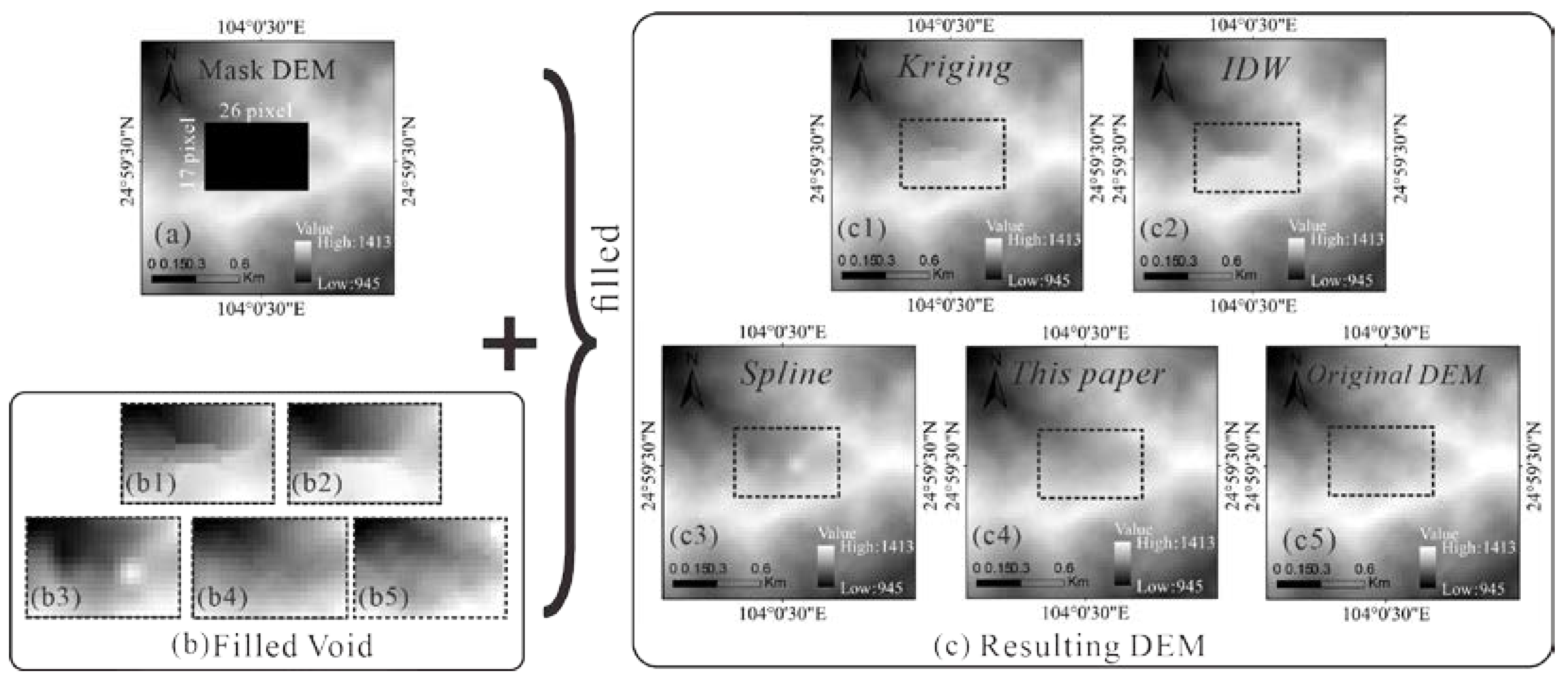
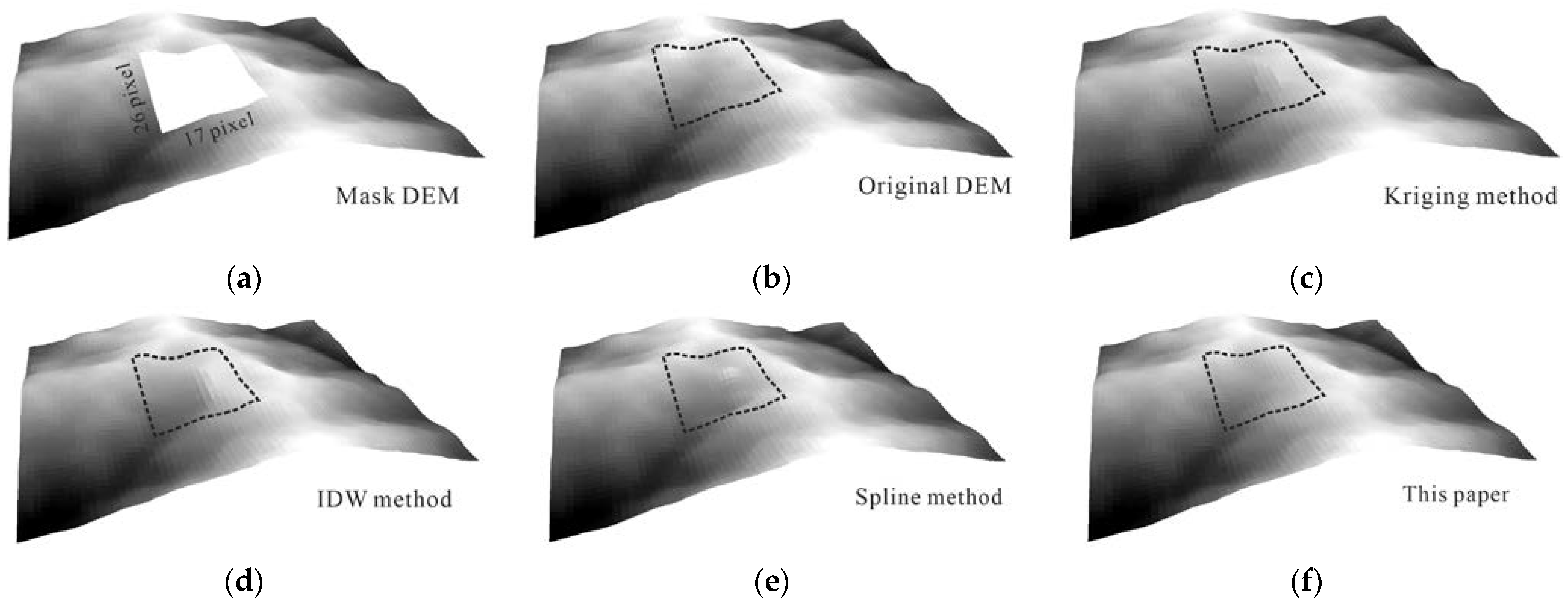
3.3. Comparison Analysis with Traditional Methods

To verify the excellence of our model, the comparison and analysis with three traditional interpolation methods, kriging, IDW, and spline interpolation, is conducted. The results are shown in Figure 11, in which a mountainous region is selected, a binary mask matrix is selected and used as the mask to fake into a DEM with a large area of voids. The maximum elevation difference is 242.47 m (the minimum elevation is 1122.95 m, and the maximum elevation is 1365.42 m). As in Figure 11a, the black rectangular area is the area to be filled. Figure 11b shows the enlargement of the filling results. Figure 11(d1–d4) show the filling results from different interpolation methods, and Figure 12 shows the 3D display of the filling results.
The experimental results show that the traditional interpolation method cannot fill large-area DEM voids; not only is the accuracy of filling low, but some topographic features generated do not match the original DEM. As shown in Figure 11(c1,c2), the filling results of kriging interpolation and inverse distance interpolation are relatively smooth, and the detailed features of the terrain are lost. Although the boundary of the filling result can be smoothly connected to the original DEM, topographic abruptness is generated in the void area. Among these, the mean error of kriging interpolation is 14.54 m, the root mean square error is 27.01 m, and the structural similarity metrics is 74.10%. The mean error of inverse distance interpolation is 19.82 m, the root mean square error is 38.04 m, and the structural similarity metrics is 61.90%. Figure 11(c3) shows that the spline interpolation method generates a relatively blurred filling result with worse terrain detail recovery and edge connection processing. The mean error of the spline interpolation is 0.27 m, the root mean square error is 21.48 m, and the structural similarity metric is 66.18%.
In addition, the model proposed in this paper is better than other traditional interpolation methods. Not only is the filling accuracy higher than that of the conventional interpolation methods, but the filling results in this paper conform to the topographic change, i.e., the filling results have a higher structural similarity with the original DEM. From the visual effect, the filling effect of our method can effectively restore the detailed features of the terrain and smoothly connect the boundary of the void with the original boundary. The MAE is 9.74 m, and the RMSE is 11.90 m. Compared with other interpolation methods, these two types of errors are the smallest. As shown in Table 3, the structural similarity metrics of our method is 84.42%. Although the PSNR values of the filling results using the traditional interpolation method are all above 20, indicating a good filling effect, the filling results do not match the original DEM in terms of visual effects.

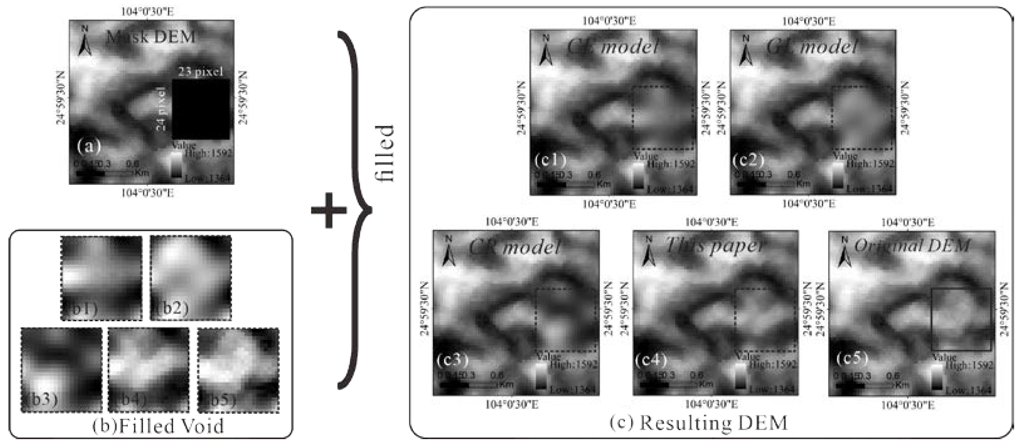
3.4. Comparison Analysis with Other Deep Learning Models

In order to further verify the excellence from our model, comparison analysis with other deep learning models, such as the CE model proposed by Pathak et al. [32], the GL model proposed by Iizuka et al. [34], and the CR model proposed by Yu et al. [42], is conducted. The results are shown in Figure 13 and Figure 14. The results for quantitative analysis are depicted in Table 4.
It can be seen from Table 4 that the PSNR values from the GL model are the smallest (16.36 dB), and PSNR values from the CE model and the CR model achieve 20.18 and 20.23 dB, respectively, while the PSNR value from the model proposed in this paper achieves 22.69 dB, which is slightly higher than that of the CE model and the CR model. In addition, as observed from Figure 13(c2,c4) and Figure 14d,f, it can be found that the filling result of DEM from the GL model is the most blurred visually compared to the results of the other three models, which are relatively clear.
Moreover, as observed from Table 4, the SSIM value from the CR model is the lowest out of the four models, which implies that the filling result of DEM only has 11.42% similarity with the original DEM (see Figure 14e), while the SSIM value from the model proposed in this paper achieved only 57.40%, which means that the filling result of DEM has 57.40% similarity with the original DEM (see Figure 14f). Other cases are between them (see Figure 14c,d). Therefore, it can be concluded that the model proposed in this paper has the highest structure similarity with the DEM surrounding the void (i.e., highest SSIM), which means that other models only obtain a relatively lower SSIM than our model does.

3.5. Discussion

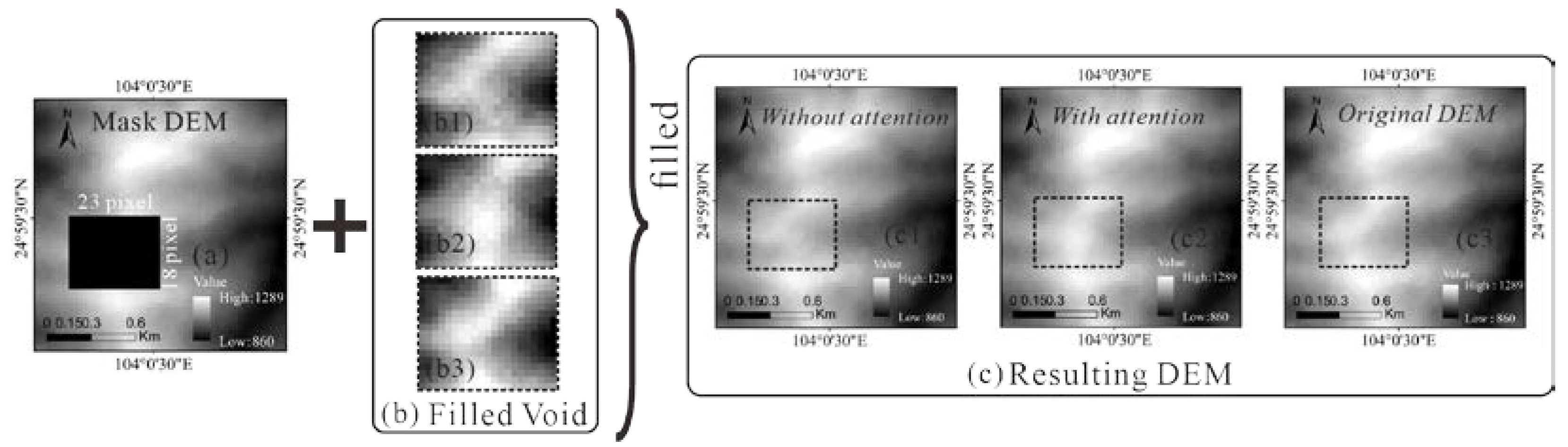
3.5.1. Impact Analysis of the Attention Mechanism vs. Filling Accuracy

To verify the effectiveness of the attention mechanism on the model proposed in this paper, the network models with and without the attention mechanism are trained separately. Each model is trained for 1000 epochs, and finally the trained models are used to fill the test data. The results are shown in Figure 15 and Table 5. It can be seen from Figure 15(c1,c2) that rich details of terrains can be achieved after adding the multiattention mechanism. Specifically, the DEM voids filled with the attention mechanism have a greater improvement than those without the attention mechanism (see Table 5). The accuracy of ME is increased by 281.25%. The accuracy of MAE and RMSE is increased by 8% and 26.5%. The accuracy of PSNR and SSIM has increased by 7.7% and 27.54%.

3.5.2. Impact Analysis of the Loss Function Type vs. Filling Accuracy

The proposed model is trained using a combined loss function, including reconstruction loss and adversarial loss. In order to verify the effect of the loss function on the filling accuracy, this paper uses reconstruction loss, adversarial loss and the combined loss as the model objective function to conduct comparative experiments. The results are depicted in Figure 16.
Figure 16 shows that the slope variation in Area 1 is relatively smooth and that the terrain is relatively simple. The effect of training with reconstruction loss and adversarial loss alone or in combined loss has little effect on the filling, and both can fill the voids with high accuracy. In Area 2, the mountain chains are connected. The filling results of the model trained separately using reconstruction loss and adversarial loss are blurred, and the terrain details are not sufficiently recovered. However, the filling results of the model obtained from the combined loss training not only fill many detailed terrain textures but also connect smoothly with the original DEM boundary. The terrain in Area 3 is more complex and contains many detailed terrain features. The experiments show that the filling results of the models trained using reconstruction loss and adversarial loss, are, respectively, very blurry, and many terrestrial details cannot be filled. Area 4 is located in a valley area, where the voids area is located at the junction between the hillside and the flat land, and the intersection is divided more clearly. The experiments show that the results from our model trained through the combined loss function can produce a consistent structural similarity with the original DEM’s. The results of the filling model trained with adversarial loss can recover more texture features of the terrain but produce abrupt changes in elevation with the original DEM, and the filling yields some redundant features. Thus, it can be concluded from the experiments that different loss functions have a great influence on the filling accuracy of the model. In contrast, the combined loss function has strong robustness, enabling the model to recover more terrain features.

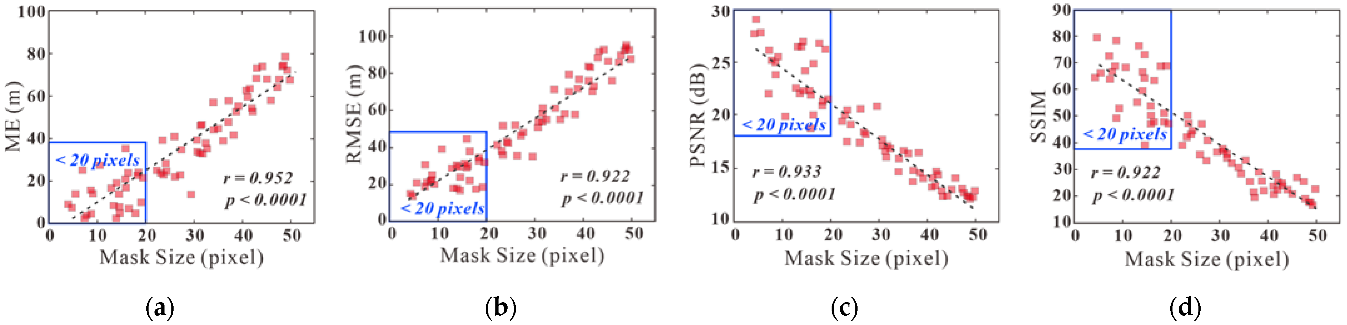
3.5.3. Impact Analysis of the Size of DEM Void vs. Filling Accuracy

The accuracy of filling DEM voids replies on the known information surrounding the DEM voids. The farther away from the void, the less the information contributes to the fill; thus, the size of the void largely determines the filling accuracy. In order to study how the size of the DEM void impacts the filling accuracy, this paper randomly generated 70 sets of masks of different sizes from 5 × 5 pixel2 to 50 × 50 pixel2, which are located in ridges and valleys. The ME, RSME, PSNR, and SSIM are calculated and shown in Figure 17. As observed from Figure 17, it can be found that the values of the PSNR and SSIM are linearly negatively relevant to the sizes of the DEM void, and the ME and RSME are linearly positively relevant to the sizes of the DEM void. Moreover, when the size of the DEM void is less than 20 × 20 pixels2, the values of the ME, RSME, PSNR, and SSIM are relatively scattered, which is caused by topographical undulations. When the size of the DEM void is bigger than 20 × 20 pixels2, the values of the ME, RSME, PSNR, and SSIM are relatively followed up by a linear increase, which means that the filling accuracy decreases linearly (see Figure 17). Therefore, it can be concluded that the model proposed in this paper can achieve the highest accuracy when the size of the DEM void is less than 20 × 20 pixels2, and the SSIM value can achieve 60%, even 80% above.

4. Conclusions

This paper proposes a multiattention generative adversarial network model to fill the DEM voids. The novelties of this paper lie in the following:
(1)
A multiscale feature fusion generation network in the model is proposed, with which the receptive field is enlarged while maintaining the density of the dilated convolution.
(2)
A channel-spatial cropping attention mechanism module is proposed for the multiattention filling network, with which the correlation between the front and back feature maps is enhanced and the global-local dependence of the feature maps is improved.
(3)
To overcome the difficulty of balancing generator and discriminator adversarial training in generative adversarial networks, this paper proposes a global-local adversarial network and uses the spectral normalization on the output of the network layer, enhancing the stability of network training as a result.
Three groups of experiments are conducted to validate the model proposed. The first group of experiments is to verify the accuracy of the model proposed in this paper. The four different types of terrains, hillsides, valleys, ridges and hills, are selected for validation. Experimental results show that the SSIM value from our model in three types of terrains, hillside, valley and ridge, can reach 80–90%. The second group of experiments is to validate the model proposed in this paper through comparison with the traditional interpolation methods, i.e., Kriging, IDW, and Spline. The experimental results show that the structural similarity from the model proposed in this paper can averagely increase by 10% when compared with the traditional four interpolation methods, i.e., Kriging, IDW, and Spline. The third group of experiments is to validate the model proposed in this paper through comparison with other deep learning models, i.e., CE, GL, and CR. The experimental results show that the SSIM value from the model proposed in this paper can reach 57.4%, while the CE, GL and CR only reach 43.05%, 17.07% and 11.42%, in hilly terrain, respectively. In addition, this paper has also discussed and analyzed the impacts of attention mechanism, loss function, and void size versus the filling accuracy of the DEM void. The experimental results from our model show that (1) the filling accuracy of the DEM void is improved by 16% after adding the attention mechanism; (2) the combined loss function when used enables the model to recover more terrain features, and the results of the filled voids have a consistent structural similarity with the original DEM’s; (3) when the void size is less than 20 × 20 pixels2, the SSIM value can reach 60–80% in the four test areas. With all of the experimental results and comparison analysis above, it can be concluded that the model proposed in this paper enables the DEM voids to be filled with higher accuracy and higher structural similarity than the traditional interpolation methods (i.e., IDW, Kriging, and Spline) and the deep learning models (i.e., CE, GL, and CR) under different terrestrial conditions.

Author Contributions

Conceptualization, G.Z. and B.S.; methodology, P.L.; software, B.S. and P.L.; validation, P.L.; writing—original draft preparation, P.L.; writing—review and editing, G.Z. and B.S.; supervision, J.X. and T.Y. All authors have read and agreed to the published version of the manuscript.

Funding

This paper is financially supported by the National Natural Science of China (grant #: 41961065), the Guangxi Innovative Development Grand Program (grant #: Guike AD19254002, GuikeAA18118038, and GuikeAA18242048), Guangxi Natural Science Foundation for Innovation Research Team (grant #: 2019GXNSFGA245001), Guilin Research and Development Plan Program (grant #: 20190210-2), the National Key Research and Development Program of China (grant #: 2016YFB0502501), Guangxi Key Laboratory of Spatial Information and Geomatics (grant#: 19-185-10-12) and the BaGuiScholars program of Guangxi.

Institutional Review Board Statement

Not applicable.

Informed Consent Statement

Not applicable.

Data Availability Statement

Not applicable.

Acknowledgments

The author would like to thank the reviewers for their constructive comments and suggestions.

Conflicts of Interest

The authors declare no conflict of interest.

References

  1. Han, H.; Zeng, Q.; Jiao, J. Quality Assessment of TanDEM-X DEMs, SRTM and ASTER GDEM on Selected Chinese Sites. Remote Sens. 2021, 13, 1304. [Google Scholar] [CrossRef]
  2. Zhou, G. Urban High-Resolution Remote Sensing Algorithms and Modeling; CRC Press, Tylor& Francis Group: Boca Raton, FL, USA, 2021; pp. 135–136. [Google Scholar]
  3. Div, A.; Aas, B. TanDEM-X DEM: Comparative performance review employing LIDAR data and DSMs. ISPRS J. Photogramm. 2020, 160, 33–50. [Google Scholar]
  4. Liu, Z.; Han, L.; Yang, Z.; Cao, H.; Guo, F.; Guo, J.; Ji, Y. Evaluating the Vertical Accuracy of DEM Generated from ZiYuan-3 Stereo Images in Understanding the Tectonic Morphology of the Qianhe Basin, China. Remote Sens. 2021, 13, 1203. [Google Scholar] [CrossRef]
  5. Sukcharoenpong, A.; Yilmaz, A.; Li, R. An Integrated Active Contour Approach to Shoreline Mapping Using HSI and DEM. IEEE T. Geosci. Remote. 2016, 54, 1586–1597. [Google Scholar] [CrossRef]
  6. Zhou, G.; Huang, J.; Zhang, G. Evaluation of the wave energy conditions along the coastal waters of Beibu Gulf, China. Energy 2015, 85, 449–457. [Google Scholar] [CrossRef]
  7. Yue, L.; Shen, H.; Yu, W.; Zhang, L. Monitoring of Historical Glacier Recession in Yulong Mountain by the Integration of Multisource Remote Sensing Data. IEEE J.-Stars 2018, 11, 1–13. [Google Scholar] [CrossRef]
  8. Zhou, G.; Bao, X.; Ye, S.; Wang, H.; Yan, H. Selection of Optimal Building Facade Texture Images From UAV-Based Multiple Oblique Image Flows. IEEE T. Geosci. Remote. 2021, 59, 1534–1552. [Google Scholar] [CrossRef]
  9. Zhou, G.; Wang, H.; Chen, W.; Zhang, G.; Luo, Q.; Jia, B. Impacts of Urban land surface temperature on tract landscape pattern, physical and social variables. Int. J. Remote Sens. 2020, 41, 683–703. [Google Scholar] [CrossRef]
  10. Maune, D.F.; Nayegandhi, A. Digital Elevation Model Technologies and Applications: The DEM Users Manual; ASPRS: Baton Rouge, LA, USA, 2019; pp. 38–39. [Google Scholar]
  11. Zhou, Q.; Liu, X. Analysis of errors of derived slope and aspect related to DEM data properties. Comput. Geosci. UK 2004, 30, 369–378. [Google Scholar] [CrossRef]
  12. Zhou, G.; Xie, M. Coastal 3-D Morphological Change Analysis Using LiDAR Series Data: A Case Study of Assateague Island National Seashore. J. Coastal Res. 2009, 25, 400–435. [Google Scholar] [CrossRef]
  13. Hirt, C. Artefact detection in global digital elevation models (DEMs): The Maximum Slope Approach and its application for complete screening of the SRTM v4. 1 and MERIT DEMs. Remote Sens. Environ. 2018, 207, 27–41. [Google Scholar] [CrossRef] [Green Version]
  14. Ma, H.; Zhou, W.; Zhang, L. DEM refinement by low vegetation removal based on the combination of full waveform data and progressive TIN densification. ISPRS J. Photogramm. 2018, 146, 260–271. [Google Scholar] [CrossRef]
  15. Uss, M.L.; Vozel, B.; Lukin, V.V.; Chehdi, K. Estimation of Variance and Spatial Correlation Width for Fine-Scale Measurement Error in Digital Elevation Model. IEEE T. Geosci. Remote 2020, 58, 1941–1956. [Google Scholar] [CrossRef]
  16. Shepard, D. A two-dimensional interpolation function for irregularly-spaced data. In Proceedings of the 1968 23rd ACM National Conference, New York, NY, USA, 27–29 August 1968; pp. 517–524. [Google Scholar]
  17. Reuter, H.I.; Nelson, A.; Jarvis, A. An evaluation of void-filling interpolation methods for SRTM data. Int. J. Geogr. Inf. Sci. 2007, 21, 983–1008. [Google Scholar] [CrossRef]
  18. Grohman, G.; Kroenung, G.; Strebeck, J. Filling SRTM voids: The delta surface fill method. Photogramm. Eng. Remote Sens. 2006, 72, 213–216. [Google Scholar]
  19. Luedeling, E.; Siebert, S.; Buerkert, A. Filling the voids in the SRTM elevation model—A TIN-based delta surface approach. ISPRS J. Photogramm. 2007, 62, 283–294. [Google Scholar] [CrossRef]
  20. Vallé, B.L.; Pasternack, G.B. Field mapping and digital elevation modelling of submerged and unsubmerged hydraulic jump regions in a bedrock step–pool channel. Earth Surf. Proc. Land. 2006, 31, 646–664. [Google Scholar] [CrossRef]
  21. Dokken, T.; Lyche, T.; Pettersen, K.F. Polynomial splines over locally refined box-partitions. Comput. Aided Geom. Des. 2013, 30, 331–356. [Google Scholar] [CrossRef]
  22. Skytt, V.; Barrowclough, O.; Dokken, T. Locally refined spline surfaces for representation of terrain data. Comput. Graph. 2015, 49, 58–68. [Google Scholar]
  23. Heritage, G.L.; Milan, D.J.; Large, A.R.; Fuller, I.C. Influence of survey strategy and interpolation model on DEM quality. Geomorphology 2009, 112, 334–344. [Google Scholar] [CrossRef]
  24. Arun, P.V. A comparative analysis of different DEM interpolation methods. Egypt. J. Remote Sens. Space Sci. 2013, 16, 133–139. [Google Scholar]
  25. Ling, F.; Zhang, Q.W.; Wang, C. Filling voids of SRTM with Landsat sensor imagery in rugged terrain. Int. J. Remote Sens. 2007, 28, 465–471. [Google Scholar] [CrossRef]
  26. Hogan, J.; Smith, W.A. Refinement of digital elevation models from shadowing cues. In Proceedings of the IEEE Conference on Computer Vision and Pattern Recognition (CVPR), San Francisco, CA, USA, 13–18 June 2010; pp. 1181–1188. [Google Scholar]
  27. Yue, T.; Chen, C.; Li, B. A high-accuracy method for filling voids and its verification. Int. J. Remote Sens. 2012, 33, 2815–2830. [Google Scholar] [CrossRef]
  28. Yue, T.; Zhao, M.; Zhang, X. A high-accuracy method for filling voids on remotely sensed XCO2 surfaces and its verification. J. Clean. Prod. 2015, 103, 819–827. [Google Scholar] [CrossRef]
  29. Yue, L.; Shen, H.; Zhang, L.; Zheng, X.; Zhang, F.; Yuan, Q. High-quality seamless DEM generation blending SRTM-1, ASTER GDEM v2 and ICESat/GLAS observations. ISPRS J. Photogramm. 2017, 123, 20–34. [Google Scholar] [CrossRef] [Green Version]
  30. Dong, G.; Chen, F.; Ren, P. Filling SRTM void data via conditional adversarial networks. In Proceedings of the IEEE International Geoscience and Remote Sensing Symposium (IGARSS), Valencia, Spain, 22–27 July 2018; pp. 7441–7443. [Google Scholar]
  31. Liu, J.; Liu, D.; Alsdorf, D. Extracting Ground-Level DEM From SRTM DEM in Forest Environments Based on Mathematical Morphology. IEEE T. Geosci. Remote 2014, 52, 6333–6340. [Google Scholar] [CrossRef]
  32. Pathak, D.; Krahenbuhl, P.; Donahue, J.; Darrell, T.; Efros, A.A. Context Encoders: Feature Learning by Inpainting. In Proceedings of the IEEE Conference on Computer Vision and Pattern Recognition (CVPR), Las Vegas, NV, USA, 27–30 June 2016; pp. 2536–2544. [Google Scholar]
  33. Guangyun, Z.; Rongting, Z.; Guoqing, Z.; Xiuping, J. Hierarchical spatial features learning with deep CNNs for very high-resolution remote sensing image classification. Int. J. Remote Sens. 2018, 39, 1–19. [Google Scholar]
  34. Goodfellow, I.; Pouget-Abadie, J.; Mirza, M.; Xu, B.; Warde-Farley, D.; Ozair, S.; Courville, A.; Bengio, Y. Generative Adversarial Networks. arXiv 2014, arXiv:1406.266. Available online: https://arxiv.org/abs/1406.2661 (accessed on 10 June 2014). [CrossRef]
  35. Iizuka, S.; Simo-Serra, E.; Ishikawa, H. Globally and locally consistent image completion. ACM Trans. Graph. 2017, 36, 107. [Google Scholar] [CrossRef]
  36. Liu, G.; Reda, F.A.; Shih, K.J.; Wang, T.C.; Tao, A.; Catanzaro, B. Image Inpainting for Irregular Holes Using Partial Convolutions. In Proceedings of the European Conference on Computer Vision (ECCV), Munich, Germany, 8–14 September 2018; pp. 85–100. [Google Scholar]
  37. Qiu, Z.; Yue, L.; Liu, X. Void Filling of Digital Elevation Models with a Terrain Texture Learning Model Based on Generative Adversarial Networks. Remote Sens. 2019, 11, 2829. [Google Scholar] [CrossRef] [Green Version]
  38. Dong, G.; Huang, W.; Smith, W.A.P.; Ren, P. A shadow constrained conditional generative adversarial net for SRTM data restoration. Remote Sens. Environ. 2020, 237, 111602. [Google Scholar] [CrossRef]
  39. Hui, Z.; Li, J.; Wang, X.; Gao, X. Image fine-grained inpainting. arXiv 2020, arXiv:2002.02609. Available online: https://arxiv.org/abs/2002.02609 (accessed on 4 October 2020).
  40. Jaderberg, M.; Simonyan, K.; Zisserman, A.; Kavukcuoglu, K. Spatial Transformer Networks. arXiv 2015, arXiv:1506.02025. Available online: https://arxiv.org/abs/1506.02025 (accessed on 4 February 2016).
  41. Hu, J.; Shen, L.; Sun, G. Squeeze-and-excitation networks. In Proceedings of the IEEE Conference on Computer Vision and Pattern Recognition (CVPR), Salt Lake City, UT, USA, 18–22 June 2018; pp. 1181–1188. [Google Scholar]
  42. Yu, J.; Lin, Z.; Yang, J.; Shen, X.; Lu, X.; Huang, T.S. Generative image inpainting with contextual attention. In Proceedings of the IEEE Conference on Computer Vision and Pattern Recognition (CVPR), Salt Lake City, UT, USA, 18–22 June 2018; pp. 5505–5514. [Google Scholar]
  43. Wang, N.; Li, J.; Zhang, L.; Du, B. MUSICAL: Multi-Scale Image Contextual Attention Learning for Inpainting. In Proceedings of the 28th International Joint Conference on Artificial Intelligence (IJCAI), Macao, China, 10–16 August 2019; pp. 3748–3754. [Google Scholar]
  44. Gavriil, K.; Muntingh, G.; Barrowclough, O.J. Void filling of digital elevation models with deep generative models. IEEE Geosci. Remote Sens. 2019, 16, 1645–1649. [Google Scholar] [CrossRef] [Green Version]
  45. Zhang, C.; Shi, S.; Ge, Y.; Liu, H.; Cui, W. DEM Void Filling Based on Context Attention Generation Model. ISPRS Int. J. Geo-Inf. 2020, 9, 734. [Google Scholar] [CrossRef]
  46. Zhu, D.; Cheng, X.; Zhang, F.; Yao, X.; Gao, Y.; Liu, Y. Spatial interpolation using conditional generative adversarial neural networks. Int. J. Geogr. Inf. Sci. 2020, 34, 735–758. [Google Scholar] [CrossRef]
  47. Li, S.; Hu, G.; Cheng, X.; Xiong, L.; Tang, G.; Strobl, J. Integrating topographic knowledge into deep learning for the void-filling of digital elevation models. Remote Sens. Environ. 2022, 269, 112818. [Google Scholar] [CrossRef]
  48. Yu, J.; Lin, Z.; Yang, J.; Shen, X.; Lu, X.; Huang, T.S. Free-form image inpainting with gated convolution. In Proceedings of the IEEE International Conference on Computer Vision (ICCV), Seoul, Korea, 27 October–2 November 2019; pp. 4471–4480. [Google Scholar]
  49. Mehta, S.; Rastegari, M.; Caspi, A.; Shapiro, L.; Hajishirzi, H. Espnet: Efficient spatial pyramid of dilated convolutions for semantic segmentation. In Proceedings of the European Conference on Computer Vision (ECCV), Munich, Germany, 8–14 September 2018; pp. 552–568. [Google Scholar]
  50. Miyato, T.; Kataoka, T.; Koyama, M.; Yoshida, Y. Spectral normalization for generative adversarial networks. arXiv 2018, arXiv:1802.05957. Available online: https://arxiv.org/abs/1802.05957 (accessed on 16 February 2018).
  51. Arjovsky, M.; Chintala, S.; Bottou, L. Wasserstein GAN. arXiv 2017, arXiv:1701.07875. Available online: https://arxiv.org/abs/1701.07875 (accessed on 26 January 2017).
  52. Kingma, D.P.; Ba, J. Adam: A method for stochastic optimization. arXiv 2017, arXiv:1412.6980. Available online: https://arxiv.org/abs/1412.6980 (accessed on 30 January 2017).
  53. Jiang, B.; Chen, G.; Wang, J.; Ma, H.; Wang, L.; Wang, Y.; Chen, X. Deep Dehazing Network for Remote Sensing Image with Non-Uniform Haze. Remote Sens. 2021, 13, 4443. [Google Scholar] [CrossRef]
  54. Wang, Z.; Bovik, A.C.; Sheikh, H.R.; Simoncelli, E.P. Image quality assessment: From error visibility to structural similarity. IEEE Trans. Image Process. 2004, 13, 600–612. [Google Scholar] [CrossRef] [PubMed] [Green Version]
Figure 1. The overall structure of the generator.
Remotesensing 14 01206 g001
Figure 2. Spatial support for void fill by receptive fields, gray-blue for known areas and white for voids to be filled. (a) K1 and K2 are ordinary convolutions with a size of 3 × 3 pixels2. For p1 pixels in the voids, part of the known area of Ω1 can be used for calculation. However, the receptive field of the p2 pixel convolution kernel cannot obtain spatial information from a known area. (b) Expanding the receptive field by increasing the size of the convolution kernel to 4 × 4 pixels2, with both p1 and p2 in the void acquiring spatial information from Ω1. (c) A rate = 2 dilated convolution is used for feature extraction, which expands the convolution kernel receptive field while reducing the parameters.
Remotesensing 14 01206 g002
Figure 3. Multiscale feature fusion module.
Remotesensing 14 01206 g003
Figure 4. Channel-spatial pruning attention (CSPA) module.
Remotesensing 14 01206 g004
Figure 5. Channel attention module.
Remotesensing 14 01206 g005
Figure 6. Spatial pruning attention module.
Remotesensing 14 01206 g006
Figure 7. Global-local adversarial network.
Remotesensing 14 01206 g007
Figure 8. (a) Xinjiang Province, (b) Heilongjiang Province, (c) Guizhou Province, and (d) Guangxi Province.
Remotesensing 14 01206 g008
Figure 9. The process of mask calculation.
Remotesensing 14 01206 g009
Figure 10. The void filling in four areas. (a1a4) is the original DEM, the black part in (b1b4) is the area to be filled, and the filling result is shown in Figure (c1c4).
Remotesensing 14 01206 g010
Figure 11. Comparison of different interpolation methods. (a) Mask DEM, (b) the filled voids with Kriging (b1), IDW (b2), Spline (b3), our method in this paper (b4), and Original DEM (b5), and (c) the resulting DEMs with Kriging (c1), IDW (c2), Spline (c3), our method in this paper (c4), and Original DEM (c5).
Remotesensing 14 01206 g011
Figure 12. Three-dimensional display of filling results. (a) Original DEM, (b) Mask DEM, (c) Kriging, (d) IDW, (e) Spline, and (f) this paper.
Remotesensing 14 01206 g012
Figure 13. Comparison analysis with the deep learning models. (a) Mask DEM, (b) the filled voids with CE model (b1), GL model (b2), CR model (b3), the proposed model (b4), and the original DEM (b5), and (c) the resulting DEMs with CE model (c1), GL model (c2), CR model (c3), the model in this paper (c4), and Original DEM (c5).
Remotesensing 14 01206 g013
Figure 14. Comparison analysis through terrestrial visualization for the filling results. (a) Original DEM, (b) Mask DEM, (c) the resulting DEMs with CE model, (d) the resulting DEMs with GL model (e) the resulting DEMs with CR model and (f) the resulting DEMs with the method in this paper.
Remotesensing 14 01206 g014
Figure 15. Comparative analysis of the attention mechanism. (a) Mask DEM, (b) the filled voids, and (c) the resulting DEMs by without attention (c1), with attention (c2), and Original DEM (c3).
Remotesensing 14 01206 g015
Figure 16. Comparison of filling results influenced by different loss functions in four areas. (a1–a4) is the original DEM, (b1b4) is the mask DEM, (c1c4) is the result of Reconstruction Loss, (d1–d4) is the result of Adversarial Loss, and (e1e4) is the result of Combined Loss.
Remotesensing 14 01206 g016
Figure 17. Variation in filling accuracy with void size: (a) ME, (b) RMSE, (c) PSNR, and (d) SSIM.
Remotesensing 14 01206 g017
Table 1. Training steps of the filling model.
Input: Original DEM, Mask matrix
Output: Initial generation of the data for G1, Refined filling data of G2, Discriminator loss value
Step 1: Dividing the original DEM into a training set, test set and setting the network training hyperparameters.
Step 2: Generating random mask masks for each DEM image to obtain simulated hole DEM images.
Step 3: When i < T do
    Sampling m samples from the training set as mini_batchsize and entering the corresponding mask matrix.
    for i < TC
      Calculating the reconstruction loss values and updating the G1 network using the Adam optimization algorithm.
    else:
      Inputting the generated image and the original image into the discriminator, calculating the adversarial loss and L2 loss values of the discriminator D, and updating the discriminator parameters.
    Finishing TC pretraining, calculating L2 reconstruction loss, adversarial loss, and updating G1, G2 and D networks using Adam optimization until training is completed and saving the model.
   end
Step 4: Sampling m sample data from the test set as mini_batchsize, randomly generating mask, inputting to the trained filling model, putting the test data through G1 and G2 networks, respectively, getting the repaired DEM images, and calculating the repair accuracy.
Table 2. Filling accuracy of results.
ME (m)MAE (m)RMSE (m)PSNR (dB)SSIM
Area 11.374.695.7729.3383.74%
Area 24.2210.1312.8033.5292.93%
Area 38.6112.2315.7928.2782.94%
Area 46.0611.8815.8521.7159.84%
Table 3. Accuracy analysis with traditional methods.
ME (m)MAE (m)RMSE (m)PSNR (dB)SSIM
Kriging14.5420.1427.0124.7674.10%
IDW19.8230.2138.0421.8061.90%
Spline0.2714.8221.4826.7766.18%
This paper2.999.7411.9031.9084.42%
The bold values are the best values for each column.
Table 4. Accuracy analysis with other deep learning models.
ME (m)MAE (m)RMSE (m)PSNR (dB)SSIM
CE3.949.6417.0220.1843.05%
GL10.8025.9734.6616.3617.07%
CR7.1317.1922.1920.2311.42%
This paper4.2013.1316.7222.6957.40%
The bold values are the best values for each column.
Table 5. Accuracy analysis with other deep learning methods.
ME (m)MAE (m)RMSE (m)PSNR (dB)SSIM
Without attention9.7613.5119.9026.6759.25%
With attention2.5612.5015.7328.7275.57%
The bold values are the best values for each column.
Publisher’s Note: MDPI stays neutral with regard to jurisdictional claims in published maps and institutional affiliations.

