Data Processing of Gravity Base Network in Plateau Area: The Case of Qinghai Province, China

Abstract

The latest gravity survey of the gravity base network in Qinghai Province, China, was conducted with six Scintrex CG gravimeters and this gravity survey was tied to existed gravity reference stations. In this gravity network with long segments and very rugged topography, the calibration of scale factors is a time-consuming progress and its accuracy may be affected by many uncertainties, and the change in drift rates of the relative gravimeters are complex over time in this long-term survey. The reasonable calculation of scale factors and drift rates plays an important role in improving the gravity estimation accuracy. In this paper, based on the least squares, robust least squares, and Bayesian methods, various parameter calculation methods were employed to process this gravity network. The performance and practicality of each method were analyzed in terms of internal and external accuracy. The results indicated that the scale factors calibrated in the baseline field had poor applicability due to insufficient gravity difference, in this case, the scale factors estimated by the adjustment models were more accurate, which weakened the correlation between gravity differences and mutual differences. The drift rates estimated by the Bayesian method were relatively smooth over time, while drift rates estimated using symmetric observations were more practical for the gravimeter with highly variable drift. The weight constraints of observations can be optimized by the robust least squares method, the gravity values obtained by it were more consistent with absolute gravity values than those obtained by the least squares method, and the robust least squares method was recommended to process gravity data in plateau areas.

1. Introduction

A gravity base network forms the basis for gravity surveys and provides accurate gravity field information for mineral resources, geotectonic inversion, geoid refinement, and geodynamic research [1,2,3,4]. China’s gravity base networks are established by relative gravity survey campaign based on a number of absolute gravity points [5]. The gravity base network of Qinghai Province, China, was established to fulfill the needs of infrastructure construction and geodesy research. The first phase of gravity measurements in this network was performed in the form of hybrid gravimetry, and five absolute gravity points and three relative gravity points were measured from 2017 to 2018. Later, in order to achieve province-wide coverage of this gravity network, the latest phase of gravity survey was conducted from September 2020 to October 2020 using two Scintrex CG-6 and four Scintrex CG-5 gravimeters.

The uncertainties of relative gravity survey mainly come from drift characteristics and scale factors of gravimeters [4]. The logistical complexity, drastic height undulations, and long distances between gravity points increased the difficulty and time required to perform gravity surveys in plateau areas. Although the calibration of scale factors was carried out in the baseline field before the gravity survey, the calibration still affected by some uncertainties such as insufficient gravity difference and the mode of transportation [6]. Scintrex CG-5 and CG-6 gravimeters with spring sensors have complex drift characteristics that may be affected by many factors, such as spring age, temperature inside instruments, and transportation [1]. Moreover, for the long-term observation, the drift rates of gravimeters vary irregularly and nonlinearly with time [7]. Therefore, effective estimation of scale factors and drift rates and optimizing weight constraints of multiple gravimeters are the major parts to ensure the processing quality of gravity data.

Traditionally, the calibration of scale factors is conducted in a well-established baseline field before the gravity survey to reduce uncertainty and the drift rate is estimated by repeating measurements for drift correction [1]. With the development of gravity data processing theory, the drift rate and scale factor of each gravimeter can be obtained using parameter estimation methods, and the corresponding adjustment models are proposed according to the different problems in gravity survey [6,7]. Hwang et al., (2002) used weighted and datum-free constraints methods to adjust relative gravity measurements in Taiwan [8]. Chen et al., (2019) proposed the Bayesian gravity network adjustment approach and derived the unconditional marginal probability density function of absolute and relative gravity observations [1]. To resolve the multiple solutions in this function, Akaike’s Bayesian information criterion (ABIC) is introduced as a minimum expense norm to estimate the optimal values of each gravimeter’s drift rate and optimize the weight of them. Wang et al., (2021) improved the Bayesian approach by introducing the scale factors of each gravimeter as new hyperparameters, so that it could both calibrate scale factors and estimate instrument drift and weight [6]. The robust least squares method decreases the effect that gross errors have on the estimation via the equivalent weight function, which converts the robust estimation to the least square estimation and the iteration method with variable weights reduces the weight of the observation with gross error [9,10,11]. Compared with the time-consuming and costly method of adding more absolute gravity observations and closed loops, the appropriate date processing method is an economical way to obtain accurate estimation of gravity. Therefore, it is desirable to analyze the suitability of different parameter estimation and adjustment models for gravity data processing in the plateau area.

In this study, we briefly described the general situation of the gravity base network in Qinghai Province, China, and its data processing methods and adjustment methods. After the pre-processing of relative gravity data and the reduction in hydrological effects on reference points, we took multiple methods to estimate scale factor, drift rate, and weight of each gravimeter, and applied the least squares, robust least squares, and Bayesian methods to adjust this gravity network. Then, the performance and practicality of those methods were evaluated by comparing the results to the absolute gravity observations. Finally, the optimum approach for the data processing of this gravity base network in plateau areas was identified.

2. Data and Methods

2.1. Study Area and Data

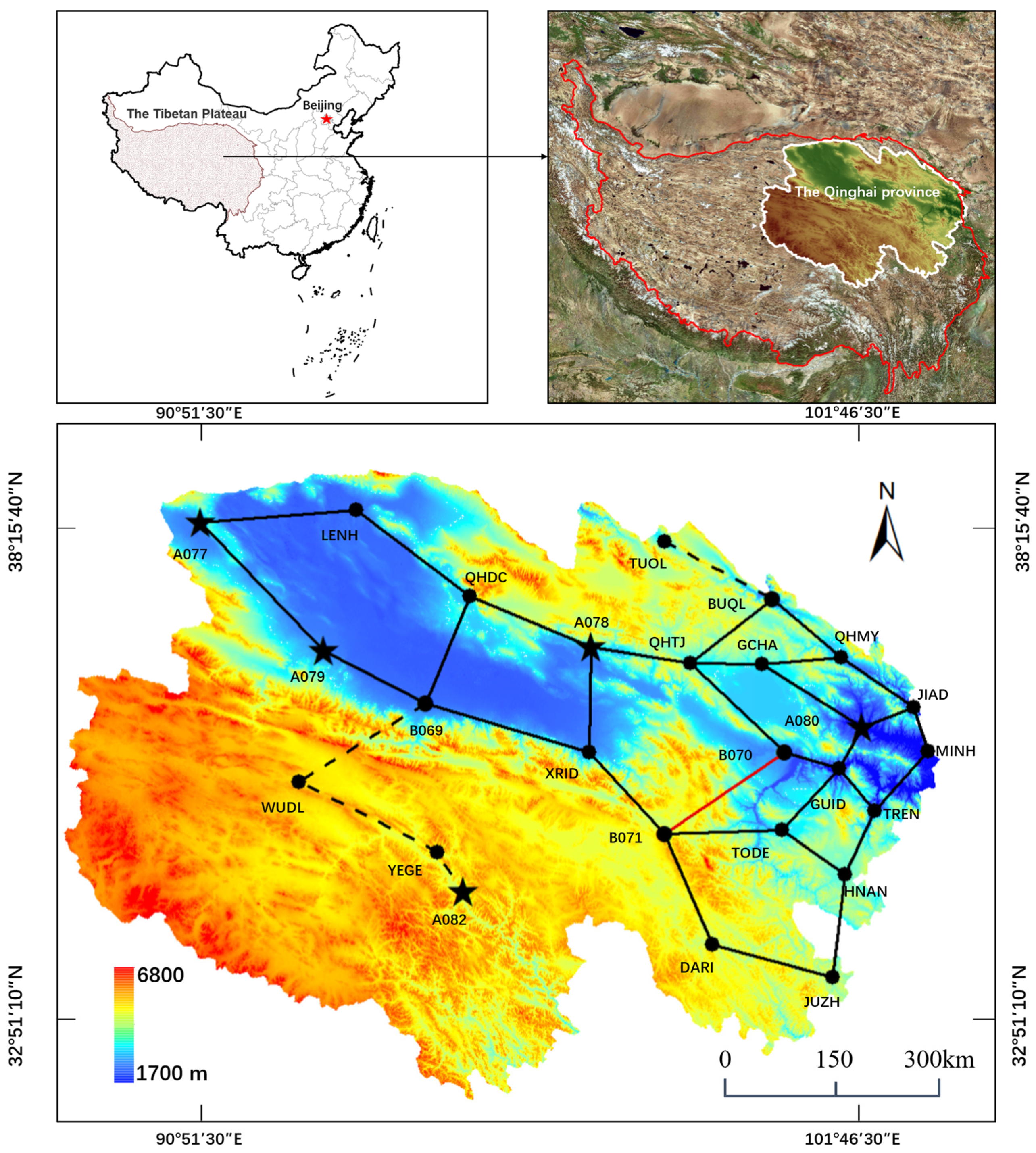
Qinghai Province is located on the northeastern Tibetan Plateau in China, with a total area of approximately 720,000 km² and an average elevation higher than 3000 m. Now the gravity base network of Qinghai Province consists of 5 absolute gravity points and 23 relative gravity points (Figure 1).

From 2017 to 2018, the first phase of gravity measurement campaigns was carried out by National Administration of Surveying, Mapping and Geoinformation of China, Xian, China. A total of 8 gravity points were obtained by the hybrid gravity survey, including 3 relative gravity points (B069, B070, and B071) and 5 absolute gravity points (A077, A078, A079, A080, and A082), which served as reference gravity points.

From September 2020 to October 2020, the latest phase of gravity survey was conducted by Jilin University, Changchun, China; Qinghai Basic Surveying; and National Administration of Surveying, Mapping and Geoinformation of China. A total of 18 new relative gravity points were measured with 2 Scintrex CG-6 and 4 Scintrex CG-5 gravimeters.

2.1.1. Absolute Gravity Instrumentation

A077, A078, A079, A080, and A082 were measured by absolute gravimeters FG5X#246 and FG5#214. FG5X#246 belongs to the Institute of Geodesy and Geophysics, Chinese Academy of Sciences (IGG CAS), Wuhan, China. FG5#214 belongs to National Administration of Surveying, Mapping, and Geoinformation of China. In order to ensure the reliability of reference and metrology, ensure the long-term stability of all gravimeters, and trace the gravity measurement to the SI, Coordination Group for Absolute Gravity Observation and Research of China was established in 2010 by three institutions: the IGG CAS; National Administration of Surveying, Mapping and Geoinformation of China; and China Earthquake Administration, Wuhan, China [12]. From 2010 to 2018, FG5X#246 and FG5#214 together with other gravimeters took part in several absolute gravity comparisons performed by this group, which provided the following offsets (

Table 1. Result of absolute gravimeter comparisons.

Gravimeter Model	Offset (μGal)
	CCAG 2013	CCAG 2015	CCAG 2018
FG5#214	−1.7 ± 2.9	−0.7 ± 1.7	−3.3 ± 1.0
FG5X#246	−1.0 ± 2.2	−0.6 ± 0.9	0.0 ± 1.4

) [12,13]:

Moreover, FG5#214 took part in the 10th International Comparison of Absolute Gravimeters (ICAG-2017), which was carried out on the Changping Campus of NIM, Beijing, China. The results showed that FG5#214 provided accurate measurements and was reliable in terms of metrology [14].

The effects of solid-earth tide, ocean tide loading, and barometric were calculated by the g9.0 software. ETGTAB model developed by Georg Wenzel was adopted to correct the effect of solid-earth tide, and FES2004 model, considered state-of-the-art, was used to correct the effect of ocean tide loading [5]. The barometric admittance factor of $-0.3 \mathsf{\mu }\mathrm{Gal}/\mathrm{hPa}$ was adopted for atmosphere correction [15,16]. The effect of vertical gravity gradient was corrected based on the measured vertical gravity gradient at each gravity points. The correction of polar motion was estimated based on the pole positions published by the International Earth Rotation and Reference Systems Service (IERS) [15].

The uncertainty of FG5X#246 and FG5#214 measurements included two components: statistical uncertainty and total systematic uncertainty, including modeling uncertainties, system uncertainties, environmental noise, set-up uncertainties, and gradient. The total uncertainty of the 5 absolute gravity points is approximately $\pm 2.5 \mathsf{\mu }\mathrm{Gal}$, which is calculated as follows [17]:

$${\Delta }_{tot}={({\delta }_{sys}^2+{\delta }_{stat}^2)}^{0.5},$$

(1)

$${\delta }_{stat}={\sigma }_{set}/\sqrt{N_{set}},$$

(2)

and

$${\Delta }_{sys}=\sqrt{{\sigma }_{bar}{}^2+{\sigma }_{pm}{}^2+{\sigma }_{et}{}^2+{\sigma }_{ol}{}^2+{\sigma }_{ls}{}^2+{\sigma }_{cl}{}^2+{\sigma }_{sm}{}^2+{\sigma }_{env}{}^2+{\sigma }_{su}{}^2+{\sigma }_{grd}{}^2},$$

(3)

where ${\delta }_{stat}$ is the statistical uncertainty, ${\sigma }_{set}$ is the set scatter (standard deviation), and $N_{set}$ is the number of sets. Here,${ \Delta }_{sys}$ is the total systematic uncertainty, consisting of four parts: (1) modeling uncertainties (barometric (${\sigma }_{bar}$), polar motion (${\sigma }_{pm}$), earth tide (${\sigma }_{et}$), ocean tide (${\sigma }_{ol}$)), (2) system uncertainties (laser (${\sigma }_{ls}$), clock (${\sigma }_{cl}$), system model (${\sigma }_{sm}$)), (3) environmental (${\sigma }_{env}$), (4) set-up uncertainties (${\sigma }_{su}$), and gradient (${\sigma }_{grd}$).

2.1.2. Hydrological Effects on Gravity

Seasonal effects of global hydrology on the first phase of gravity measurements were removed before adjustment. The effects were divided into loading and gravitational parts, the calculation was divided into several areas according to the spherical distance between the mass and the measurement point, and the contribution of each area was calculated using the formula provided by Farrell [18]. In this study, the GLDAS model was used to calculate the effect of global land water on reference points (

Table 2. Effect of global land water on gravity points.

Gravity Points	Measured Time	Gravimeter Model	Effect of Hydrology (µGal)
A082	August 2018	FG5X#246	−1.7
A077	June 2017	FG5#214	−0.7
A079	July 2018	FG5X#246	−0.8
A078	July 2018	FG5X#246	−1.2
A080	July 2017	FG5X#246	0.5
B070	November 2018	LCR-G	−0.3
B071	August 2018	Scintrex CG-5	1.1
B069	August 2018	Scintrex CG-5	0.9

). The effects of hydrology are as follows:

$$g^E\left(\psi \right)=-\frac{g}{M}{{\displaystyle \sum }}_{n=0}^{\infty }\left(2h_n-\left(n+1\right)k_n\right)P_n\left(cos\psi \right)$$

(4)

and

$$g^N\left(\psi \right)=\frac{g}{4Msin\left(\psi /2\right)},$$

(5)

where $\psi$ is the spherical distance between the mass and the measurement point, $g^E\left(\psi \right)$ is the loading effect per unit mass, $g^N\left(\psi \right)$ is the gravitational effect per unit mass, $g$ represents the mean surface gravity, $M$ represents the mass of the Earth, $h_n$ and $k_n$ represent the load Love numbers, and $P_n$ represent the Legendre polynomials.

2.1.3. Relative Gravity Survey

The latest phase of the gravity survey lasted nearly 45 days. A total of 404 measurements were obtained using 6 relative gravimeters (2 Scintrex CG-6, and 4 Scintrex CG-5) on 35 segments, which included 10 closed loops (the maximum segment number of loops was 5), 1 annexed gravimetric line (B069-WUDL-YEGE-A082), and 1 branch line (BUQL-TUQL) (

Table 3. Closing of the gravimetric polygons in this gravity survey.

Closed Loop	Segment Number	Deviation of the Gravimetric Polygon (µGal)	Permitted Deviation for Polygon (µGal)
B069-A079-A077-LENH-QHDC-B069	5	7.2	44.7
B069-XRID-A078-QHDC-B069	4	9.6	40.0
XRID-B071-B070-QHTJ-A078-XRID	5	−22.8	44.7
B071-B070-GUID-TODE-B071	4	−16.9	40.0
B071-DARI-JUZH-HNAN-TODE-B071	5	−7.8	44.7
HNAN-TODE-GUID-TREN-HNAN	4	−1.0	40.0
TREN-MINH-JIAD-A080-GUID-TREN	5	−1.1	44.7
A080-GCHA-QHTJ-B070-GUID-A080	5	0	44.7
A080-JIAD-QHMY-GCHA-A080	4	12.9	40.0
QHTJ-GCHA-QHMY-BUQL-QHTJ	4	−8.9	40.0

). The 6 relative gravimeters were checked regularly, and performance tests were carried out on all gravimeters before gravity survey according to technology standard [19].

A080 and A082 were most suitable for the calibration with a gravity difference of approximately 700 mGal, which could cover the entire measurement range. However, the distance between A080 and A082 was excessive. To consider traffic, time consumption and economic factors, all relative gravimeters were calibrated in B070 and B071. The calibration line covered a gravity difference of approximately 430 mGal (Figure 1). The calibration line followed the road between B070 and B071 with a distance of 270 km, and the travel time of interval was less than 4 h, enabling the calibration to be completed within one day.

At each gravity point, the gravimeters were set for 3–5 min before data collection to obtain the data measured by gravimeters at steady state. The data collection required 5 series of 60 one-second measurements. Symmetrical survey scheme ($A-B-C\cdots \cdots C-B-A$) was applied, and each loop was closed within 48 h. The geodetic coordinates and altitude of the gravity points were surveyed based on the Qinghai CORS and the refined local geoid of Qinghai (root mean square (RMS) of 10 cm).

2.2. Relative Gravity Data Preprocess

Tide force causes periodic changes in the gravity value at each points, thus requiring the removal of its influence [20]. Longman formulas were used to correct the effect, which are expressed as follows [21]:

$${\delta }_{gb}=-\left[{\delta }_{th}G\left(t\right)-{\delta }_{fc}\right],$$

(6)

$$\begin{gathered} G\left(t\right)=-165.17F\left(\phi \right){(c_m/r_m)}^3\left(co{s}^2{Z}_m-\frac{1}{3}\right)-1.37F^2\left(\phi \right){(c_m/r_m)}^4 \\ \times cos{Z}_m\left(5co{s}^2{Z}_m-3\right)-76.08F\left(\phi \right){(c_s/r_s)}^3\left(co{s}^2{Z}_s-\frac{1}{3}\right), \end{gathered}$$

(7)

$${\delta }_{fc}=-4.83+15.73si{n}^2{\phi }^{\prime }-1.59si{n}^4{\phi }^{\prime },$$

(8)

and

$$F\left(\phi \right)=0.998327+0.00167cosa,$$

(9)

where ${\delta }_{gb}$ (${10}^{-8}{ \mathrm{ms}}^{-2}$) is the correction value for the solid-Earth tide; ${\delta }_{th}$ is the tide factor, which was taken as 1.16; $c_m$ is the average distance from the geocenter to the selenocenter; $r_m$ is the distance from the selenocenter to the geocentric; $c_s$ is the average distance from the geocenter to the heliocenter; $r_s$ is the distance from the geocentric to the heliocentric; $Z_m$ is the geocentric zenith distance from the Moon to the gravity station; $Z_s$ is the geocentric zenith distance from the sun to the gravity station; $\phi$ is the latitude of the gravity station; and ${\phi }^{\prime }$ is the geocentric latitude of the station.

The Earth’s atmospheric density decreases with an increasing altitude, such that gravity is affected by changes in the atmospheric quality and by deformation of the Earth [22,23]. The study area is located in the plateau area with an average elevation exceeding 3000 m; the elevations of some gravity points exceed 5000 m, which requires an atmospheric correction [24]:

$${\delta }_{g_a}=0.3\left(p-p_n\right)$$

(10)

and

$$p_n=1.01325\times {10}^3{(1-\frac{0.0065\times H}{288.15})}^{5.2559},$$

(11)

where ${\delta }_{ga}$ (${10}^{-8}{ \mathrm{ms}}^{-2}$) is the air pressure correction;$p$ ($\mathrm{hPa}$) is the measured air pressure at the gravity station, which ranges from 630$\mathrm{hPa}$ to 817$\mathrm{hPa}$ in this survey;$p_n$ (${10}^{-8}{ \mathrm{ms}}^{-2}$) is the standard pressure at the gravity station; and $H$ (m) is the elevation of the gravity station.

To obtain the gravity values on the ground, the correction of each point is as follows [25]:

$${\delta }_{g_h}=\theta \times h,$$

(12)

where $\theta$ is the vertical gravity gradient (${10}^{-8} {\mathrm{s}}^{-2}$) measured at each point and $h$ is the height of the gravimeter sensor with an original fixed tripod.

2.3. Scale Factor and Drift Correction

The scale factors can be calibrated using the baseline field or obtained as unknown parameters in the adjustment process [26] as follows:

$$C=\Delta G_{12}/\Delta g_{12},$$

(13)

where $\Delta G_{12}$ is the difference in the known gravity values between two gravity points and $\Delta g_{12}$ is the average gravity difference measured by the relative gravimeter between two gravity points [27]. The method of using the adjustment model to estimate the scale factor is described in the adjustment model. In addition to calibration using the baseline field, the scale factors were estimated by the adjustment model.

The drift rate of the relative gravimeter is calculated as follows:

$$k=\frac{g-g^{\prime }}{t-t^{\prime }},$$

(14)

where $g$ (${10}^{-8 }{\mathrm{ms}}^{-2}$) and $g^{\prime }$ are the round-trip observations at the starting point of the survey line and $t$ and $t^{\prime }$ are the corresponding moments of the round-trip measurement at the starting point of the survey line.

The drift correction for the gravity observation can be calculated as follows:

$$\delta g_k=k\times \Delta t,$$

(15)

where $\delta g_k$ is the drift correction value, $k$ is the drift rate, and $\Delta t$ is the time interval between the observation station and the starting point.

In the above model, the drift rate of each relative gravimeter was calculated using the symmetrical observations. In addition, we also adopted the Bayesian approach, whose prior assumption is that the variation in the drift rate is smooth throughout the gravity survey for any relative gravimeter in good condition. The Bayesian approach applies ABIC to estimate the optimal variance of each relative gravimeter and the variances for variations of each drift, thus the drift rate of each time period can be obtained [1]. The simplex method can speed up the ABIC minimization process and improve the computational efficiency [28,29].

2.4. Adjustment of the Gravity Network

2.4.1. Classic Least Squares Adjustment

The error equation for the relative gravity observation can be written as:

$$\begin{gathered} V_{ij}=g_j-g_i+{\displaystyle \sum }_{K=1}^M\left(g_{RZi}^K-g_{RZj}^K\right)\cdot C_K+{\displaystyle \sum }_{n=1}^N{X}_n\left(cos\frac{R_i\cdot 2\pi }{T_n}-cos\frac{R_j\cdot 2\pi }{T_n}\right) \\ +{{\displaystyle \sum }}_{n=1}^N{Y}_n(sin\frac{R_i\cdot 2\pi }{T_n}-sin\frac{R_j\cdot 2\pi }{T_n}), \end{gathered}$$

(16)

where $g_i$ and $g_j$ are the gravity adjustment values of points $i$ and $j$, respectively; $g_{RZi}$ and $g_{RZj}$ are the preprocessed values of points $i$ and $j$, respectively, after the solid-Earth tide correction, air pressure correction, instrument high correction, and drift correction; $R_i$ and $R_j$ are the readings of the gravimeter at points $i$ and $j$, respectively, $C_K$ is the $K$-th grid value correction factor of the M-th degree polynomial lattice value function of the gravimeter; $N$ is the number of period terms; $X_n$ and $Y_n$ are the periodic error parameters of the relative gravimeter; and $T_n$ is the period of the period error.

The weight of the relative gravity observations can be obtained using Helmert variance components estimation. If $M$ denotes the number of relative gravimeters, the variance components, i.e., ${\sigma }^2={\left[{\sigma }_1^2\cdots {\sigma }_M^2\right]}^T$ can be calculated as follows [30]:

$$\left[\begin{array}{c}\begin{array}{c}{\sigma }_I^2\\ {\sigma }_I^2\end{array}\\ ⋮\\ {\sigma }_M^2\end{array}\right]={\left[\begin{array}{cccc}{U}_1{U}_1& U_1{U}_2& \cdots & U_1{U}_M\\ U_2{U}_1& U_2{U}_2& \cdots & U_2{U}_M\\ ⋮& ⋮& \ddots & ⋮\\ U_M{U}_1& U_M{U}_2& \cdots & U_M{U}_M\end{array}\right]}^{-1}\left[\begin{array}{c}\begin{array}{c}{V}_1^T{P}_1{V}_1\end{array}\\ V_2^T{P}_2{V}_2\\ \cdots \\ V_M^T{P}_M{V}_M\end{array}\right]$$

(17)

and

$$\{\begin{array}{c}{U}_I{U}_I=m_I-2tr\left(N^{-1}{N}_I\right)+tr{\left(N^{-1}{N}_I\right)}^2\\ U_I{U}_J=tr\left(N^{-1}{N}_I{N}^{-1}{N}_I\right),\left(I\ne J\right)\end{array},$$

(18)

where $P_I \left(I=1,2,\cdots ,M\right)$ is the weight matrix for each relative gravimeter’s observations, $V_I$ is the residual vector of each relative gravimeter calculated by the adjustment, $N_I$ is the normal equation of each relative gravimeter, $N$ is the overall normal equation, and $m_I$ is the number of measurements from the $I$-th gravimeter. The steps in the Helmert variance components estimation are as follows. First, the relative gravity observations from each gravimeter were adjusted according to the equal weight treatment. The weights were then determined according to the posterior variance in the observations from each gravimeter, after which adjustment was performed again according to the posterior weights, repeating the above process until the unit weight medium error of the different observation types tends to be consistent [31].

The error equation for the a priori gravity value is as follows [8]:

$$V_i=g_i-g_i^0,$$

(19)

where $V_i$ is the residual of the gravity value at point $i \mathrm{and} g_i^0$ and $g_i$ are the priori gravity value with weight matrix $P_g$ and its adjustment value at point $i,$ respectively. Combining Equations (13) and (16) yielded the following [8]:

$$V=AX-L,$$

(20)

where $L$ and $V$ are the gravity measurements and the residuals vector, respectively, $A$ is the design matrix, $X$ is the unknown gravity vector at all stations.

The unbiased estimation of the unknown parameters is:

$$X=N^{-1}{A}^{T}PA,$$

(21)

where P is the weight matrix, P = diag (P_I, P_g). The calibrated scale factors of the baseline field are generally calculated before the adjustment of the gravity network. When calibrating scale factors in the survey area, certain phenomena may exist, such as insufficient gravity difference, excessively long survey line, and inconvenient traffic may exist. In this survey, reference gravity points were evenly distributed and there are a large number of redundant observations, which provides the feasibility to estimate reliable scale factors through adjustment model.

2.4.2. Robust Least Squares Adjustment

The robust least squares estimation can weaken the impact that gross errors have on the adjustment [32,33]. The error equation for the gravity observation with a weight of $p_i$ is as follows:

$$v_i=a_{i}X-L_i,$$

(22)

The criteria for the robust estimation is [9]:

$${{\displaystyle \sum }}_{i=1}^n{p}_i\rho \left(v_i\right)=min,$$

(23)

where $\rho \left(v_i\right)$ is the convex function of $v_i$, let ${\rho }^{\prime }\left(v_i\right)=\psi \left(v_i\right)$, the equivalent weight of ${\overline{p}}_i$, which changes with the standardized residuals in the iterative calculation, is as follows [34]:

$${\overline{p}}_i=p_i\frac{\psi \left(v_i\right)}{v_i},$$

(24)

The initial values of ${\widehat{X}}^{\left(0\right)}$,$V^{\left(0\right)},$ and ${\widehat{\sigma }}_{v_i}$ were obtained using the least squares method. The $\left(k+1\right)$th solution of the robust estimation can be obtained after the determination of the $\left(k+1\right)$th equivalent weight:

$${\widehat{X}}^{\left(k+1\right)}=(A^T{\overline{P}}^{\left(k+1\right)}A{)}^{-1}{A}^T{\overline{P}}^{\left(k+1\right)}L,$$

(25)

The difference between two consecutive solutions of the same unknown parameter is $({\widehat{x}}_j^{k+1}-{\widehat{x}}_j^k)$. The iteration stops until $max\left|{\widehat{x}}_j^{k+1}-{\widehat{x}}_j^k\right|<\epsilon$, where $\epsilon$ is the threshold. Commonly used equivalent weight models include the Huber estimation [9], Danish method [35], IGG method [36], and Hampel three-tailed estimation [37]. The IGG III method was applied in this study, and the equivalent weight model was as follows [38]:

$${\overline{p}}_i=\{\begin{array}{c}{p}_i,\left|v_i^{\prime }\right|=\left|\frac{v_i}{{\sigma }_{v_i}}\right|\le k_0\\ p_i\frac{k_0}{\left|v_i^{\prime }\right|}(\frac{k_1-\left|v_i^{\prime }\right|}{k_1-k_0}{)}^2,k_0<\left|v_i^{\prime }\right|\le k_1\\ 0,\left|v_i^{\prime }\right|>k_1\end{array},$$

(26)

where $k_0$ and $k_1$ are the thresholds and $\left|v_i^{\prime }\right|$ is the standardized residual. The IGG III method divides the observations into three parts: the observations with standardized residuals less than $k_0$ retain their original weights; the weights of observations with standardized residuals from $k_0$ to $k_1$ are reduced; and the observations with standardized residuals greater than $k_1$ are eliminated. The values of $k_0$ and $k_1$ are 1.5 and 4.5, respectively, in this study. The scale factors can be substituted into the error equation as unknown parameters for estimation.

2.4.3. Bayesian Adjustment

The Bayesian approach can estimate the variance of gravity observation noise and the variance of drift rate to determine the weights and drift rates of all gravimeters [1].

Assuming that the observation noise obeys a normal distribution and the variation in the drift rate is smooth, the relative gravity observation equation of gravimeter $p$, the absolute gravity observation equation, and the a priori assumption of drift rate of gravimeter $p$ can be expressed by the following model:

$$A_{p}x+D_p{v}_p-y_p~N\left(0,W_p^{-1}\right),$$

(27)

$$Gx-g~N\left(0,W_g^{-1}\right),$$

(28)

and

$$B_p{v}_p~N(0,W_{b,p}^{-1}),$$

(29)

where $A_p$ is the coefficient matrix corresponding to gravimeter $p$, $D_p$ is composed of the time interval between two adjacent gravity points for gravimeter $p$, $v_p$ is the drift rate vector for gravimeter $p$,$y_p$ is the vector derived from the observations of gravimeter $p$, $W_p$ is the weight matrix of gravimeter $p$, $G$ is the coefficient matrix related to the absolute gravity observations, $W_g$ is the weight diagonal matrix of the absolute gravity, $B_p$ is a second-order smooth matrix, and $W_{b,p}$ is the weight matrix of the drift rate variations for gravimeter $p$ [1].

Combining Equations (24) and (26) for all gravimeters with Equation (25), we obtained:

$$SX-Y~N(0,{\tilde{W}}^{-1}),$$

(30)

where

$$S=\left[\begin{array}{cc}A& D\\ G& 0\\ 0& B\end{array}\right], X=\left[\begin{array}{c}x\\ v\end{array}\right], Y=\left[\begin{array}{c}\begin{array}{c}y\\ g\end{array}\\ 0\end{array}\right], \tilde{W}=\left[\begin{array}{ccc}W& 0& 0\\ 0& W_g& 0\\ 0& 0& W_b\end{array}\right].$$

(31)

The ABIC serves as an additional constraint, which is expressed as follows [1]:

$$\begin{gathered} ABIC=logdet{\left(\begin{array}{cc}W& 0\\ 0& W_a\end{array}\right)}^{-1}+logdet{S}^T\tilde{W}S-logde{t}^{+}\left(2\pi B^T{W}_{b}B\right) \\ +log min\left[U\left(X\right)\right]+2H, \end{gathered}$$

(32)

where $U\left(X\right)=SX-Y^T\tilde{W}\left(SX-Y\right)$ and $H$ is the number of super parameters. The simplex optimization algorithm was used to increase the speed of the ABIC minimization in this study [28]. Each instrument observation noise variance and drift rate variance estimated by the ABIC minimization criterion are combined with the known absolute gravity observation variance to form the weight matrix, $\tilde{W}$ [1]. The estimation of the unknown parameters can be expressed as follows:

$$\tilde{X}=\left[\begin{array}{c}\tilde{x}\\ \tilde{v}\end{array}\right]={(S^T\tilde{W}S)}^{-1}{S}^T\tilde{W}Y,$$

(33)

where $\tilde{x}$ is the estimation of the gravity value, $\tilde{v}$ is the estimation of the drift rate of all the gravimeters, and the scale factor of each gravimeter can be used as hyper-parameters to obtain its optimal value using the ABIC minimization criterion [39].

3. Analysis Procedures and Results

After the pre-processing of absolute and relative gravity data, the unknown parameters were estimated using the classic least squares method, robust least squares method and Bayesian approach. The characteristics of the different methods, used to determine the scale factors, drift rates, and weights, were analyzed. The applicability of the different methods for processing gravity conjunction data in plateau areas was analyzed.

3.1. Free Network Adjustment and Compatibility Test of Known Points

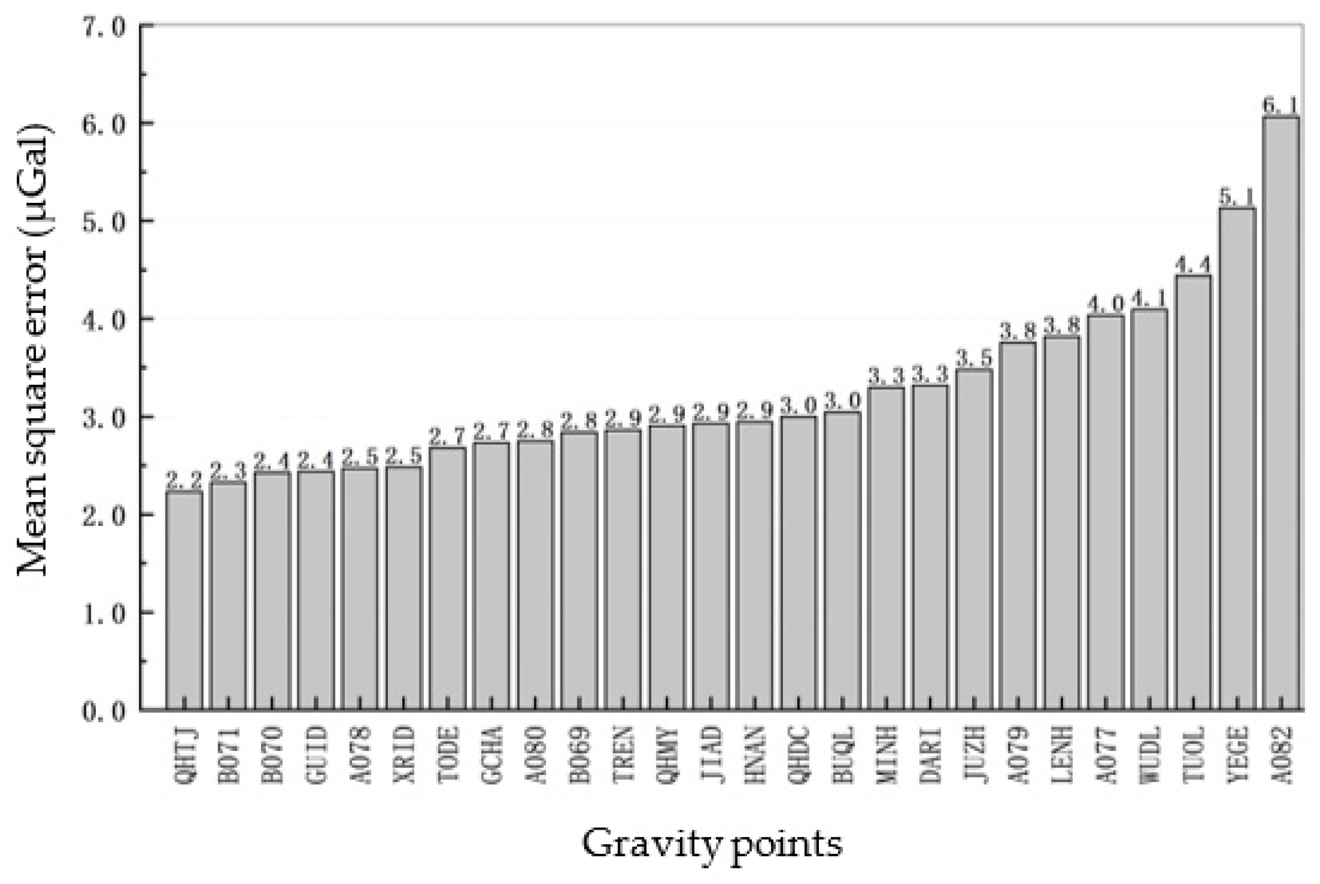
Free network adjustment evaluates the observation quality of the gravity network using the internal accord accuracy (Figure 2). The results indicated that the gravity points with the highest accuracy were mostly distributed at the largest closed loop of the gravity network (B070, GUID, TODE, GCHA, and A080) or at the edge of the largest closed loop of the gravity network connected with multiple gravity points (QHTJ, B071, A078, XRID, B069, TREN, QHMY, JIAD, HNAN, QHDC, and BUQL). The gravity points located at the edge of the largest closed loop of the gravity network that merely connected with two gravity points indicated a slightly lower accuracy (A077, LENH, A079, JUZH, DARI, and MINH). Gravity points with the lowest accuracy were located at the annexed route or in the branch line of Qilian-Tuole (A082, YEGE, WUDL, and TUQL). F test was used to test the compatibility of known points by adjusting the gravity network into two groups, the first group is free network adjustment and the second group is the least squares adjustment involving known points. After adjustments of the two groups, the subsample variance of the first group was calculated as: $m_1^2=\left[P{V}_1{V}_1\right]/r_1$ = 243.4, $r_1=377$ and that of the second group was calculated as: $m_2^2=\left[P{V}_2{V}_2\right]/r_2$ = 275.6, $r_1=386$. Using F test to analyze the influence of known points:

(1)

$H_0:{\sigma }_1^2={\sigma }_2^2$,

(2)

$F_0=\frac{m_2^2}{m_1^2}=1.10$,

(3)

let significance level: $\alpha =0.10$, then $F_{\alpha }=1.14$, $F_0<F_{\alpha }$, and the null hypothesis holds, so the known gravity points are compatible.

3.2. Scale Factor

In the adjustment where all of the reference points participate, the scale factors of each gravimeter were estimated by the classic least squares method, robust least squares method, and Bayesian approach. A slight difference existed in the scale factors for the same gravimeter when estimated by these methods, with a maximum difference of $1\times {10}^{-5}$. However, the difference between the calibrated and estimated scale factors for gravimeters C259, C262, and C284 reached $5\times {10}^{-5}$, the calibrated scale factor is less than one and the estimated scale factors were all greater than one for the C262 gravimeter (

Table 4. Scale factors of the six relative gravimeters based on different adjustment methods.

Serial No. of Gravimeters	Gravimeter Model	Scale Factors
		Baseline Field	Least Squares	Robust Least Squares	Bayesian Approach
C259	Scintrex CG-6	1.000007	1.000062	1.000061	1.000059
C262	Scintrex CG-6	0.999996	1.000046	1.000046	1.000043
C283	Scintrex CG-5	0.999612	0.999642	0.999642	0.999638
C284	Scintrex CG-5	0.999608	0.999659	0.999659	0.999656
C298	Scintrex CG-5	1.000627	1.000625	1.000624	1.000620
C617	Scintrex CG-5	0.999489	0.999504	0.999510	0.999500

). As such, further analysis was needed to discriminate the accuracy of the calibrated and estimated scale factors.

The inaccuracy of the scale factors may lead to the existence of systematic errors in gravity differences because the gravity differences are multiplied by the corrected observations and the scale factor. For two gravimeters, if there is unequal error in their scale factors, mutual difference (i.e., the difference between the two gravity differences measured by them in the same section) will be correlated with the corresponding gravity difference. The mutual differences for two gravimeters with accurate scale factors follow a random distribution, which means they are independent of gravity differences.

When using the calibrated scale factors, a correlation was discovered between the mutual differences in the two gravimeters and gravity differences, and the slant linear fitting results indicated that the mutual differences relate to the value range of the gravity differences (Figure 3a,b). This phenomenon is related to the insufficient gravity differences in the baseline field. As the max gravity difference is about 600 mGal, and the gravity difference in the baseline field (430 mGal) could not cover the range of gravimeter readings in the survey area. The residual systematic errors may remain in the calibrated scale factors. When using the estimated scale factors, the correlation between the mutual differences and gravity differences was significantly lower; the range of the mutual differences became smaller, and the linear fitting result had an approximately zero slope (Figure 3a,b). Based on the random distribution of the mutual differences, it can be seen that the systematic errors were completely corrected.

The optimal accuracy of the estimated scale factors was obtained when all reference gravity points participated in the adjustment. Different numbers and distributions of the control points (i.e., reference gravity points used in the adjustment as initial-data) may affect the estimation of the scale factors (

Table 5. Scale factors for different adjustment methods using different reference points.

Reference Points (Elevation Difference)	Serial No. of Gravimeters	Scale Factors
		Least Squares	Robust Least Squares	The Bayesian Approach
A080 and A077 (540 m)	C259(CG-6)	1.000415	1.000416	0.998272
	C262(CG-6)	1.000399	1.000400	0.998292
	C283(CG-5)	0.999995	0.999998	0.997840
	C284(CG-5)	1.000012	1.000016	0.998028
	C298(CG-5)	1.000977	1.000977	0.998809
	C617(CG-5)	0.999856	0.999865	0.997826
A080 and A082 (1800 m)	C259(CG-6)	1.000083	1.000082	1.000067
	C262(CG-6)	1.000067	1.000066	1.000054
	C283(CG-5)	0.999663	0.999664	0.999642
	C284(CG-5)	0.999679	0.999682	0.999666
	C298(CG-5)	1.000645	1.000643	1.001391
	C617(CG-5)	0.999524	0.999531	0.999498
A080, A082, and A079 (1800 and 1400 m)	C259(CG-6)	1.000070	1.000070	1.000071
	C262(CG-6)	1.000054	1.000055	1.000065
	C283(CG-5)	0.999650	0.999652	0.999651
	C284(CG-5)	0.999667	0.999670	0.999666
	C298(CG-5)	1.000633	1.000632	1.000633
	C617(CG-5)	0.999512	0.999522	0.999511

). When A080 (Xining, China) and A077 (Mangya, China), with the lowest gravity difference, were set as the control points, the scale factors estimated by the Bayesian approach were all less than one, significantly different than those controlled by all of the reference gravity points. The scale factors estimated by the classic least squares and robust least squares methods showed a difference of approximately $3.5\times {10}^{-4}$ compared to the scale factors controlled by all the reference gravity points. When A080 (Xining, China) and A082 (Qumalai, China), with the greatest gravity difference, were set as the control points, a relative higher difference occurred as compared with the Bayesian approach controlled by all of the reference gravity points; a scale factor difference of $2\times {10}^{-5}$ was observed between the least squares and robust least squares methods. When A080 (Xining, China), A082 (Qumalai, China), and A079 (Geermu, China) were set as the control points, the estimated scale factors showed a difference of approximately $1.5\times {10}^{-5}$ compared to those of the Bayesian approach controlled by all reference points; the differences were approximately $8\times {10}^{-6}$ and $1\times {10}^{-5}$ for the gravimeters using the classic least squares and robust least squares methods, respectively. The Bayesian approach was the most sensitive to the number of control points; the estimated parameters indicated a poorer accuracy when adjustments were controlled by a smaller number of control points. The classic least squares and robust least squares methods indicated no significant differences when the adjustment was controlled by the same points; an increase in either the number of control points or the gravity differences may improve the accuracy of scale factors.

The accuracy and reliability of the adjustment can be verified by some of the reference points not set as control points. Taking A080 (Xining, China) and A082 (Qumalai, China) as the control points, the network was adjusted by the least squares method using the scale factors listed in Table 5. The adjusted gravity values reached a discrepancy of 69.1 μGal on A079 using the scale factors calculated by A080 (Xining, China) and A077 (Mangya, China), while the discrepancy significantly decreased on A079, A078, and A077 when using the scale factors calculated by A080 (Xining) and A082 (Qumalai, China). The discrepancy decreased further when using the scale factors calculated by A080 (Xining), A082 (Qumalai, China), and A079 (Geermu, China). The adjustment had the optimal accuracy using the scale factors calculated at all of the reference points, with the largest discrepancy of 19.4 µGal (

Table 6. Discrepancy between the adjusted gravity values calculated by different estimated scale factors and the check points.

Check Points	Discrepancy between Adjusted Gravity Values and Check Gravity Values (μGal)
	Scale Factors Obtained by A080 and A077	Scale Factors Obtained by A080 and A082	Scale Factors Obtained by A080, A082, and A079	Scale Factors Obtained by All Reference Points
A079	69.1	22.3	20.6	19.4
A078	23.7	−6.1	−7.3	−8.0
A077	95.5	12.2	9.1	7.0

). In summary, the gravity difference, quantity, and spatial distribution of the control points notably influenced the accuracy of the estimated scale factors, and the highest accuracy scale factors were estimated using the maximum number of control points, the greatest gravity differences, and the most widely distributed stations.

3.3. Drift Correction

We used the symmetrical observation mode and conducted measurements between gravity points A and C as follows: $A-B-C\cdots \cdots C-B-A$, and the drift rates can be calculated based on the field data surveyed by frequently returning to the starting points. After corrections for the solid-Earth tide, air pressure, instrument height, and drift, the corrected relative gravity difference was used in the classic least squares and the robust least squares adjustments. The Bayesian approach assumes that the variation in the drift rate varies as a nonlinear smooth function with the elapsed time, and the optimal values of the drift rate variances were estimated based on ABIC.

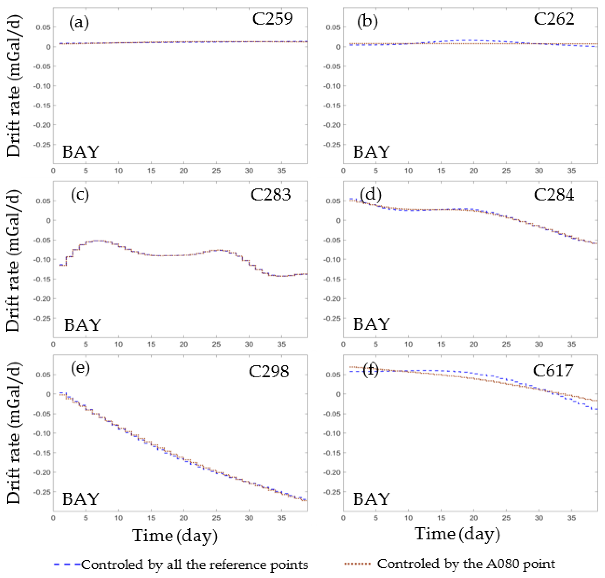
Figure 4 showed the estimated drift rate of each gravimeter adjusted by the Bayesian approach controlled by all the reference points and that calculated by the symmetric observations. The drift rate estimated by the Bayesian approach gently changed with time, whereas the change in the drift rate was irregularly based on the symmetric observations. C259 and C262 showed the lowest drift rate less than $0.04 \mathrm{mGal}/\mathrm{d}$, and the estimated drift rate difference between the Bayesian approach and that the symmetric observations can be nearly neglected (Figure 4a,b). The estimated drift rate of C283 by the Bayesian approach significantly differed to the symmetric observations, which reached $0.13 \mathrm{mGal}/\mathrm{d}$ on some days (Figure 4c).

For gravimeters C284, C298, and C627, an identical time trend for the estimated drift rate was obtained by the Bayesian approach and the symmetric observations and the drift rate calculated by the symmetric observations significantly undulated over several days (Figure 4d–f).

The drift rate estimated by Bayesian adjustment controlled by reference point A080 was compared to the drift rate controlled by all reference points (Figure 5), it can be seen that the maximum difference was less than $0.015 \mathrm{mGal}/\mathrm{d}$ on C259, C262, and C298 (Figure 5a,b,e), while C283, C284, and C617 indicated similar drift rates (Figure 5c,d,f).

The Bayesian adjustment simultaneously estimated the gravity values of the network and the drift rates. The classic least squares method obtained the gravity values after the observations were corrected by the drift rate calculated using the symmetric observations. The estimations of hyper parameters using A079, A082, B070, and A077 as the control points were similar to those using all of the reference points. When A079, A082, B070, and A077 were used as the control points and all gravity observations participated in the adjustment, the two types of discrepancies obtained by two methods, respectively, have negligible difference within 3.0 μGal (

Table 7. Discrepancies between the adjustment gravity values obtained using different drift rates and the check points (all observations participated in the adjustment).

Check Points	Discrepancy between Adjusted Gravity Values and Check Points (µGal)
	Using Drift Rates Estimated by the Bayesian Approach	Using the Drift Rates Estimated by the Symmetric Observations
A080	−19.1	−20.0
A078	−22.2	−22.0

). Generally, there was negligible difference between the adjustment results of the two methods when all gravity observations participated in the adjustment. C283 showed a difference of $0.14 \mathrm{mGal}/\mathrm{d}$ in the drift rates between the Bayesian approach and that using the symmetric observations on some days (Figure 6). The classic least squares method showed better performance than the Bayesian approach because the unsmooth variations at C283 were significantly inconsistent with the smooth hypothesis of the Bayesian approach (

Table 8. The discrepancy between the adjusted gravity values obtained by using different drift rates and the check points (only the observations of C283 participated in the adjustment).

Check Points	Discrepancy between Adjustment Gravity Values and Check Points (µGal)
	Using the Drift Rates Estimated by the Bayesian Approach	Using the Drift Rates Estimated by the Symmetric Observations
A080	−6.8	−2.7
A078	−19.0	−13.4

).

3.4. Weights

Gravity differences usually cannot be regarded as equal-precision observations, the variance component estimation was used to obtain the variance of each gravimeter given the nominal accuracy of Scintrex CG-6 gravimeter was better than Scintrex CG-5, and the results indicated that gravimeters C259 and C262 had smaller posterior variances (

Table 9. Posterior variances and weights of each gravimeter obtained via the variance component estimation.

Serial No. of Gravimeter	Gravimeter Model	Posterior Variances	Weight
C259	Scintrex CG-6	0.000125	3.19
C262	Scintrex CG-6	0.000112	3.57
C283	Scintrex CG-5	0.000311	1.28
C284	Scintrex CG-5	0.000240	1.66
C298	Scintrex CG-5	0.000336	1.19
C617	Scintrex CG-5	0.000399	1.00

).

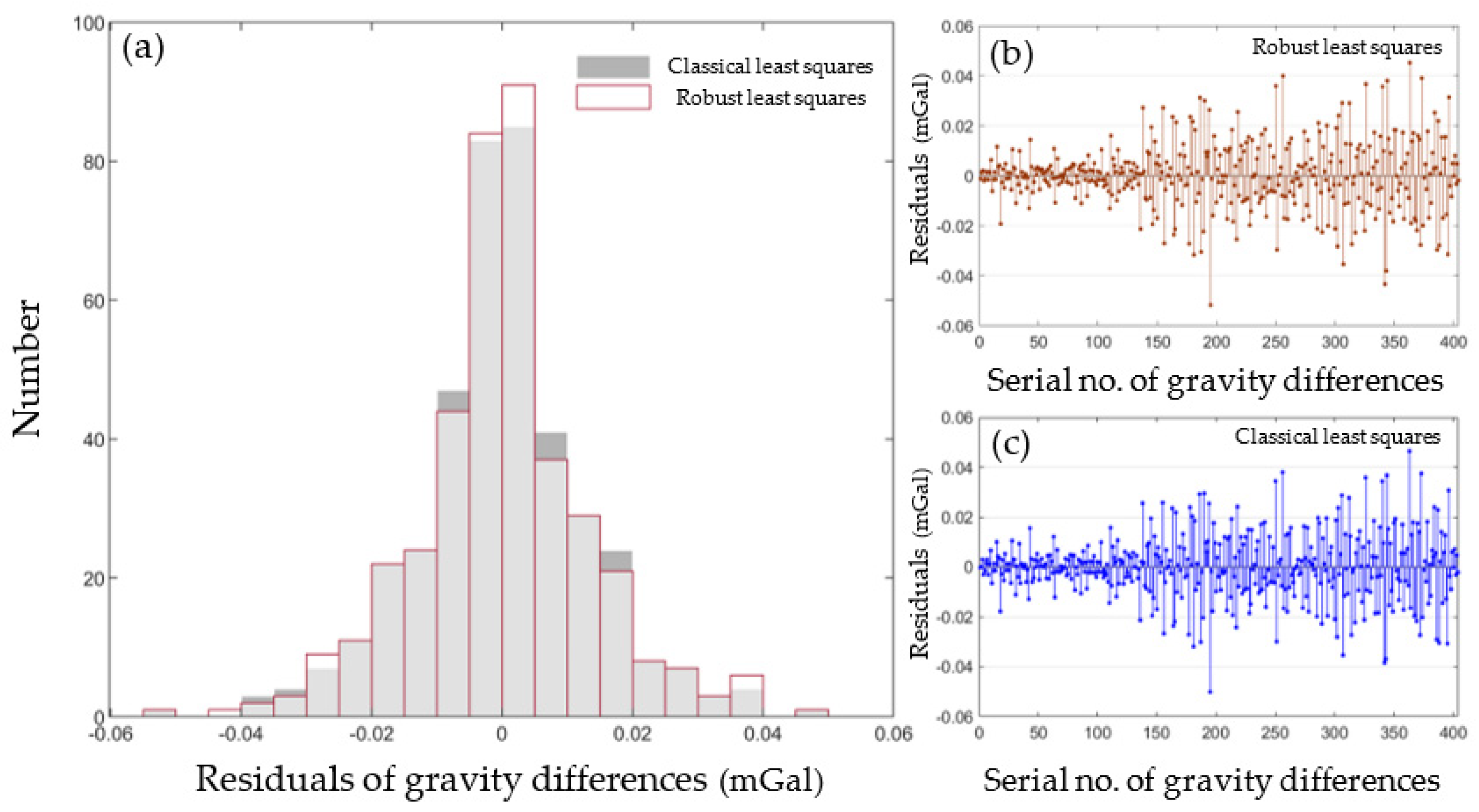
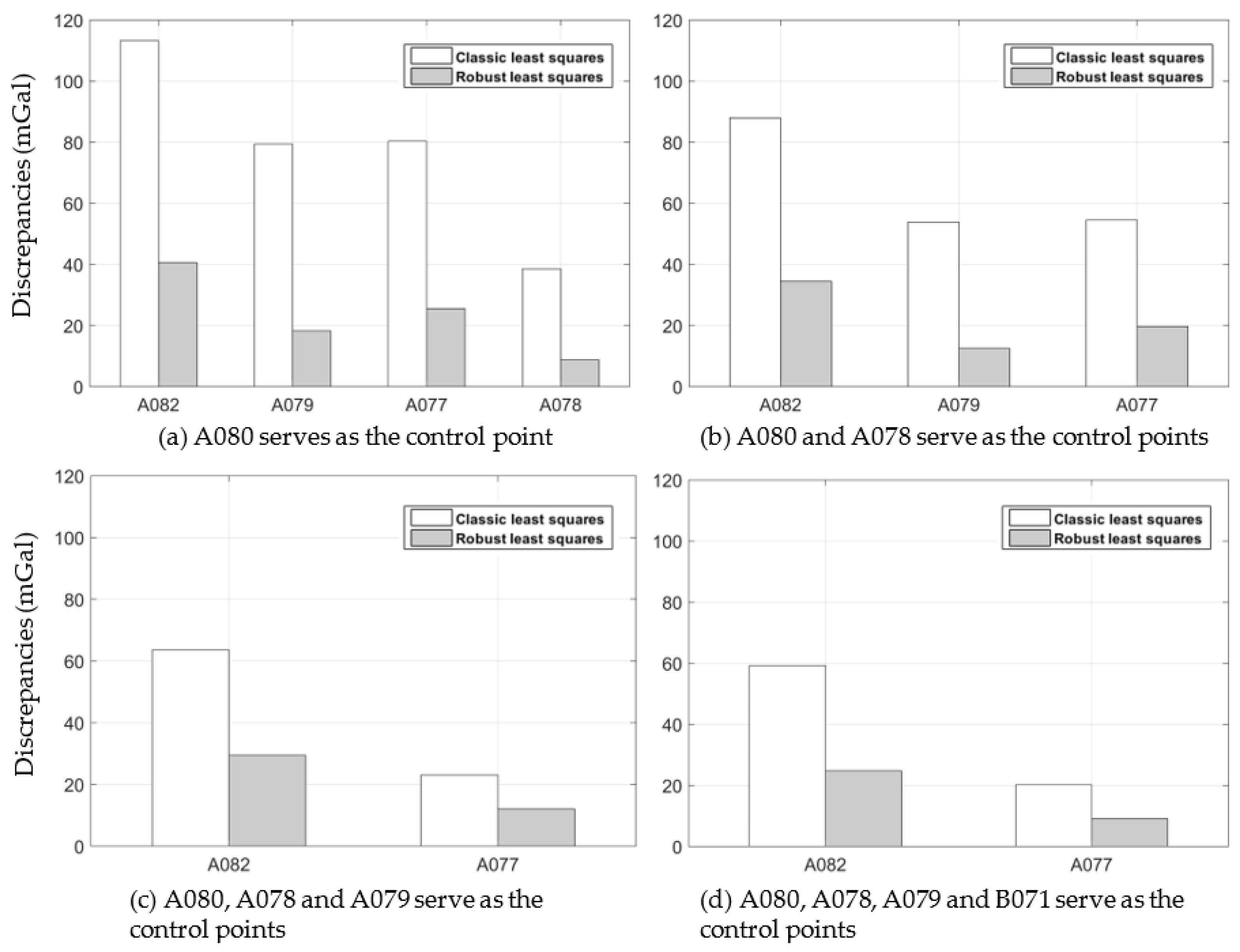
Several high-precision gravimeters were involved in this survey and the gravity observations showed a high precision and no observation was eliminated when the robust least squares adjustment method was used. The residuals of the gravity differences obtained by the least squares method and robust least squares method all obey normal distribution (Figure 7), and the adjusted gravity values obtained by the least squares and the robust least squares methods indicated negligible numerical difference (within 2 µGal). For the convenience of discussion, parts of the reference points were used as control points and the others were used as checkpoints to test the reliability of the robust least squares method.

The observations of C259 and C262 were taken as examples for adjustment, and gross error (threefold the mean square error) was added in some observations of C259 (B069-WUDL, B069-A079, B069-XRID, and GUID-B070). We designed four groups of schemes to test the performance of the least squares method and robust least squares method (

Table 10. Test schemes of the performance of the least squares method and robust least squares method.

Schemes	Control Points	Checkpoint
a	A080	A077, A078, A079, and A082
b	A080 and A078	A077, A079, and A082
c	A080, A078, and A079	A077, and A082
d	A080, A078, A079, and B071	A077, and A082

). In terms of the discrepancies between the adjusted gravity values and check points, the result of the robust least squares method is better than the least squares method (Figure 8). When A080 was used as the control point, the discrepancies between the adjusted gravity values and the check points obtained by the least squares method ranged from 39 to 113 μGal. Compared to the least squares method, the discrepancies obtained by the robust least squares method ranged from 9 to 41 μGal. When A080 and A078 were used as the control points, the discrepancies obtained by the two methods were significantly reduced compared to the result obtained by only one control point; however, the result of the least squares method still had a discrepancy higher than 50 μGal at A082, A079, and A077 (Figure 8b). When A080, A078, and A079 were used as control points, the discrepancies at A077 near A079 decreased significantly, by 31 μGal for the least squares method and 8 μGal for the robust least squares method (Figure 8c). When A080, A078, A079, and B071 are used as control points, the accuracy of the two methods was improved slightly (Figure 8d). The adjustment results obtained by the robust least squares method are more accurate in the case of gross error.

The ABIC minimization can estimate the scale factor of each relative gravimeter with high accuracy, as well as estimating the optimal value of the observational noise variances to determine the weight of each gravimeter.

Table 11. Observational noise variances estimated by the ABIC.

Serial No. of Gravimeters	Gravimeter Model	Variances	Weight
C259	Scintrex CG-6	0.0000179	7.70
C262	Scintrex CG-6	0.0000167	8.29
C283	Scintrex CG-5	0.0001518	0.91
C284	Scintrex CG-5	0.0001085	1.27
C298	Scintrex CG-5	0.0001181	1.17
C617	Scintrex CG-5	0.0001381	1.00

showed the observational noise variance of each gravimeter estimated by ABIC. Taking the weight estimated by ABIC as the initial weight, the robust adjustment weighted by ABIC yielded slightly more accurate adjustment values than those weighted by the variance component estimation (

Table 12. Discrepancies between the adjusted gravity values calculated by the robust least squares method using different initial weights and the values of check points.

Control Points	Check Points	Discrepancy between Adjustment Values and Check Points (µGal)
		Using the Weights by the Variance Component Estimation	Using the Weights by the ABIC
A078	A077	15.9	17.2
	A079	28.4	24.8
	A080	2.8	1.5
	A082	23.8	20.0
A079	A077	12.5	7.6
	A078	28.4	24.8
	A080	25.6	23.3
	A082	4.6	4.8
A080	A077	13.1	15.7
	A078	−2.8	−1.5
	A079	25.6	23.3
	A082	21.1	18.5

).

4. Discussion

Gravity networks located in plateau areas present challenging field survey conditions. In this study, six high-precision relative gravimeters were used for symmetric observations and eight reference gravity points distributed across the study area (Qinghai Province, China) were used as reference points. The data processing results using multiple methods indicate the sound accuracy of the network.

The scale factors played an important role in gravity data processing; multiple methods for the definition of each gravimeter’s scale factor were applied in this study because the calibration was highly difficult owing to the large variations in elevation in this area. Although the scale factor of each instrument was calibrated in the baseline prior to the gravity observation, the calibrated scale factors had poor suitability owing to the insufficient gravity difference in the calibration field. Systematic errors were found in the calibrated scale factors through a gravity difference in the simultaneous observation gravimeters and gravity difference in two adjacent stations. The estimated scale factors reduced the correlation between the mutual differences and gravity differences. The scale factors estimated by the three adjustment models were all more accurate than those calibrated by the baseline field with insufficient gravity differences.

The drift rates of the Bayesian approach and the least squares method using the symmetric observations showed similar accuracies when all observation stations were involved in the adjustment. This can be attributed to the high precision of the field survey and the nearly equal drift rates estimated by the Bayesian approach and by using symmetric observations. The variation in the drift rates at C283, which had poor stability, was not smooth owing to transportation, temperature, and other uncertainty factors arising from the plateau environment, which contradicted the prior assumptions of the Bayesian approach. When the observations of gravimeter C283 were merely involved in the classic least squares adjustment, the accuracy was significantly higher than that of the Bayesian approach, indicating that field observations are more accurate for complex drift undulation.

The equivalent weight of each observation calculated by the robust least squares method appeared to be more reasonable. This method weighted the observations with different precision by the same gravimeter, which reduced the effect of possible gross errors and yielded more reliable adjustment results.

The uncertainty of the terrestrial relative gravity observation mainly derived from the drift and scale factors of the gravimeters. All three adjustment models performed well in estimating the scale factors; a more reliable drift rate for the gravimeter was calculated using the symmetric observations. For gross error, the least squares adjustment result was significantly affected by gross error, whereas the robust least squares method performed best for gravity network adjustments in plateau areas.

5. Conclusions

This study applied the classic least squares, robust least squares, and Bayesian adjustment methods for gravity data processing in plateau areas, Qinghai Province, China. Using the different approaches, we estimated the scale factors, drift rates, and weights. The conclusions of this study can be summarized as follows:

• Scale factors calibrated by the baseline field have poor applicability in this gravity survey due to the insufficient gravity difference in the calibration field. When a large number of the control points with large gravity differences are across the study area, the scales factors estimated by the adjustment model also have high accuracy.
• The gravimeter drift rates estimated by the Bayesian approach showed a high accuracy for gravimeters with a smooth drift rate, while the drift rate calculated by the field symmetric observations indicated better performance for the gravimeters with low drift stability.
• The robust least squares method weighted by the ABIC with the scale factors as the unknown parameters showed the best performance, and the Bayesian and classic least squares methods showed similar adjustment accuracy.

References

1. Chen, S.; Zhuang, J.; Li, X.; Lu, H.; Xu, W. Bayesian approach for network adjustment for gravity survey campaign: Methodology and model test. J. Geod. 2018, 93, 681–700. [Google Scholar] [CrossRef] [Green Version]
2. Chapman, D.S.; Sahm, E.; Gettings, P. Monitoring aquifer recharge using repeated high-precision gravity measurements: A pilot study in South Weber, Utah. Geophysics 2008, 73, WA83–WA93. [Google Scholar] [CrossRef] [Green Version]
3. Timmen, L.; Gerlach, C.; Rehm, T.; Volksen, C.; Voigt, C. Geodetic-Gravimetric Monitoring of Mountain Uplift and Hydrological Variations at Zugspitze and Wank Mountains (Bavarian Alps, Germany). Remote Sens. 2021, 13, 23. [Google Scholar] [CrossRef]
4. Yang, J.; Chen, S.; Wang, L.; Lu, H.; Li, H.; Zhang, B. Data quality assessment of time-varying terrestrial gravity observation in South China. Acta Geod. Cartogr. Sin. 2021, 50, 333–342. (In Chinese) [Google Scholar] [CrossRef]
5. Xing, L.L.; Bai, L.; Niu, X.W.; Sang, P. A new and high-precision gravity base network in the south of the Tibetan Plateau. Geod. Geodyn. 2020, 11, 258–264. [Google Scholar] [CrossRef]
6. Wang, L.H.; Chen, S.; Zhuang, J.C.; Xu, W.M. Simultaneous calibration of instrument scale factor and drift rate in network adjustment for continental-scale gravity survey campaign. Geophys. J. Int. 2022, 228, 1541–1555. [Google Scholar] [CrossRef]
7. Yang, J.L.; Chen, S.; Zhang, B.; Zhuang, J.C.; Wang, L.H.; Lu, H.Y. Gravity Observations and Apparent Density Changes before the 2017 Jiuzhaigou Ms7.0 Earthquake and Their Precursory Significance. Entropy 2021, 23, 20. [Google Scholar] [CrossRef]
8. Hwang, C.W.; Wang, C.G.; Lee, L.H. Adjustment of relative gravity measurements using weighted and datum-free constraints. Comput. Geosci. 2002, 28, 1005–1015. [Google Scholar] [CrossRef] [Green Version]
9. Huber, P.J. Robust estimation of location parameter. Ann. Math. Stat. 1964, 35, 492–518. [Google Scholar] [CrossRef]
10. Baselga, S. Global optimization solution of robust estimation. J. Surv. Eng. 2007, 133, 123–128. [Google Scholar] [CrossRef]
11. Touati, F.; Kahlouche, S.; Idres, M. Robust and Efficient Weighted Least Squares Adjustment of Relative Gravity Data. In Proceedings of the IAG International Symposium on Gravity, Geoid and Earth Observation 2008, Khania, Greece, 23–27 June 2008; pp. 59–65. [Google Scholar]
12. Zhang, X.; Han, Y.; Wang, J.; Shen, C.; Hu, M.; Wang, J.; Li, Z. Comparisons of Absolute Gravimeters Measurements from Crustal Movement Observation Network of China during 2010 and 2018. Earthq. Res. China 2020, 36, 872–878. [Google Scholar] [CrossRef]
13. Li, J.; Li, H.; Zhang, S.; He, Z.; Zhang, W.; Ji, L.; Xia, C. Results of the Second Contrast Observation of Absolute Gravimeters (CCAG-2013). J. Geod. Geodyn. 2014, 34, 64–66. [Google Scholar] [CrossRef]
14. Wu, S.Q.; Feng, J.Y.; Li, C.J.; Su, D.W.; Wang, Q.Y.; Hu, R.; Mou, L.S. The results of 10th International Comparison of Absolute Gravimeters (ICAG-2017). J. Geod. 2021, 95, 16. [Google Scholar] [CrossRef]
15. Palinkas, V.; Lederer, M.; Kostelecky, J.; Simek, J.; Mojzes, M.; Ferianc, D.; Csapo, G. Analysis of the repeated absolute gravity measurements in the Czech Republic, Slovakia and Hungary from the period 1991-2010 considering instrumental and hydrological effects. J. Geod. 2013, 87, 29–42. [Google Scholar] [CrossRef]
16. Merriam, J.B. Atmospheric pressure and gravity. Geophys. J. Int. 1992, 109, 488–500. [Google Scholar] [CrossRef] [Green Version]
17. Greco, F.; Riguzzi, F.; Berrino, G. Insights into Seismogenetic Areas in Central Italy from Combined Absolute Gravity and GNSS Measurements. Remote Sens. 2021, 13, 25. [Google Scholar] [CrossRef]
18. Mikolaj, M.; Meurers, B.; Guntner, A. Modelling of global mass effects in hydrology, atmosphere and oceans on surface gravity. Comput. Geosci. 2016, 93, 12–20. [Google Scholar] [CrossRef] [Green Version]
19. GB/T 20256-2019; Specifications for the Gravimetry Control. Standard Press of China: Beijing, China, 2019.
20. Lederer, M. Accuracy of the Relative Gravity Measurement. Acta Geodyn. Geomater. 2009, 6, 383–390. [Google Scholar]
21. Longman, I.M. Formulas for computing the tidal accelerations due to the moon and the sun. J. Geophys. Res. 1959, 64, 2351–2355. [Google Scholar] [CrossRef]
22. Boy, J.P.; Gegout, P.; Hinderer, J. Reduction of surface gravity data from global atmospheric pressure loading. Geophys. J. Int. 2002, 149, 534–545. [Google Scholar] [CrossRef] [Green Version]
23. Hinderer, J.; Riccardi, U.; Rosat, S.; Boy, J.P.; Hector, B.; Calvo, M.; Littel, F.; Bernard, J.D. A study of the solid earth tides, ocean and atmospheric loadings using an 8-year record (2010–2018) from superconducting gravimeter OSG-060 at Djougou (Benin, West Africa). J. Geodyn. 2020, 134, 11. [Google Scholar] [CrossRef]
24. Medved, K.; Kuhar, M.; Koler, B. Regional gravimetric survey of central Slovenia. Measurement 2019, 136, 395–404. [Google Scholar] [CrossRef]
25. Hipkin, R.G. Absolute determination of the vertical gradient of gravity. Metrologia 1999, 36, 47–52. [Google Scholar] [CrossRef]
26. Dias, F.; Escobar, I.P. A model for adjustment of differential gravity measurements with simultaneous gravimeter calibration. J. Geod. 2001, 75, 151–156. [Google Scholar] [CrossRef]
27. Onizawa, S. Apparent calibration shift of the Scintrex CG-5 gravimeter caused by reading-dependent scale factor and instrumental drift. J. Geod. 2019, 93, 1335–1345. [Google Scholar] [CrossRef]
28. Nelder, J.A.; Mead, R. A Simplex-Method for Function Minimization. Comput. J. 1965, 7, 308–313. [Google Scholar] [CrossRef]
29. Akaike, H. Bayesian-Analysis of Minimum Aic Procedure. Ann. Inst. Stat. Math. 1978, 30, 9–14. [Google Scholar] [CrossRef]
30. Zhang, P.F.; Tu, R.; Gao, Y.P.; Zhang, R.; Liu, N. Improving the Performance of Multi-GNSS Time and Frequency Transfer Using Robust Helmert Variance Component Estimation. Sensors 2018, 18, 13. [Google Scholar] [CrossRef] [Green Version]
31. Yang, Y.X.; Xu, T.H.; Song, L.J. Robust estimation of variance components with application in global positioning system network adjustment. J. Surv. Eng. 2005, 131, 107–112. [Google Scholar] [CrossRef]
32. Hogg, R.V. Introduction to Robust and Quasi-Robust Statistical Methods (Book). J. Am. Stat. Assoc. 1985, 80, 784. [Google Scholar] [CrossRef]
33. Osada, E.; Borkowski, A.; Kurpinski, G.; Oleksy, M.; Seta, M. Fitting a Precise Levelling Network to Control Points Using a Modified Robust Huber’s Mean Error Function. J. Surv. Eng. 2017, 143, 6. [Google Scholar] [CrossRef]
34. Yu, H.; Shen, Y.; Yang, L.; Nie, Y. Robust M-estimation using the equivalent weights constructed by removing the influence of an outlier on the residuals. Surv. Rev. 2019, 51, 60–69. [Google Scholar] [CrossRef]
35. Hassan, K.M.Z. Comparative evaluation among various robust estimation methods in deformation analysis. Spat. Inf. Res. 2016, 24, 485–492. [Google Scholar] [CrossRef]
36. Song, X.G.; Jiang, Y.; Shan, X.J.; Qu, C.Y. Deriving 3D coseismic deformation field by combining GPS and InSAR data based on the elastic dislocation model. Int. J. Appl. Earth Obs. Geoinf. 2017, 57, 104–112. [Google Scholar] [CrossRef]
37. Hampel, F.R. Influence Curve and Its Role in Robust Estimation. J. Am. Stat. Assoc. 1974, 69, 383–393. [Google Scholar] [CrossRef]
38. Yang, Y.; Song, L.; Xu, T. Robust estimator for correlated observations based on bifactor equivalent weights. J. Geod. 2002, 76, 353–358. [Google Scholar] [CrossRef]
39. Wang, L.; Chen, S.; Zhuang, J.; Lu, H.; Zhang, B.; Yang, J. Bayesian estimation of the scale factor of relative gravimeter in precise gravity survey. Acta Geod. Cartogr. Sin. 2020, 49, 1543–1553. (In Chinese) [Google Scholar] [CrossRef]
Figure 1. Distribution of the gravity points in Qinghai Province, China. Pentacles indicate the reference gravity points measured by absolute gravimeters and circles indicate the relative gravity points. Black solid lines show the closed loops of the gravimetric lines. Black-dashed lines show the branch route while the red solid line showed the gravity calibration line.
Remotesensing 14 01142 g001
Figure 2. Mean square error of the gravity values based on free network adjustment.
Remotesensing 14 01142 g002
Figure 3. Mutual differences and gravity differences for two gravimeters per set obtained using the estimated and calibrated scale factors, respectively. (a): mutual differences and gravity differences for C298 and other gravimeters. (b): mutual dif-ferences and gravity differences for C617 and other gravimeters.
Remotesensing 14 01142 g003
Figure 4. Drift rates for all gravimeters calculated using symmetric observations and with the Bayesian approach. (af): drift rates for gravimeters C259, C262, C283, C284, C298 and C617.
Remotesensing 14 01142 g004
Figure 5. Drift rates estimated by the Bayesian approach with different number of control points. (af): drift rates for gravimeters C259, C262, C283, C284, C298 and C617.
Remotesensing 14 01142 g005
Figure 6. Drift rates of all gravimeters by the symmetric observations and the Bayesian approach. (af): drift rates for gravimeters C259, C262, C283, C284, C298 and C617.
Remotesensing 14 01142 g006
Figure 7. The residuals of the gravity differences from the least squares method and the robust least squares methods: (a) Histograms of the both kinds of residuals. (b) Residuals of gravity differences obtained by the least squares method. (c) Residuals of gravity differences obtained by the robust least squares method.
Remotesensing 14 01142 g007
Figure 8. Discrepancies between the adjusted gravity values and the values of reference points.
Remotesensing 14 01142 g008