Article

CO Fluxes in Western Europe during 2017–2020 Winter Seasons Inverted by WRF-Chem/Data Assimilation Research Testbed with MOPITT Observations

1
Shanghai Carbon Data Research Center, Key Laboratory of Low-Carbon Conversion Science & Engineering, Shanghai Advanced Research Institute, Chinese Academy of Sciences, Shanghai 201210, China
2
University of Chinese Academy of Sciences, Beijing 100049, China
3
Urban Public Safety Research Center, Shanghai Advanced Research Institute, Chinese Academy of Sciences, Shanghai 201210, China
*
Author to whom correspondence should be addressed.
Remote Sens. 2022, 14(5), 1133; https://doi.org/10.3390/rs14051133
Submission received: 21 November 2021 / Revised: 13 February 2022 / Accepted: 22 February 2022 / Published: 25 February 2022

Abstract

:
The study of anthropogenic carbon monoxide (CO) emissions is crucial to investigate anthropogenic activities. Assuming the anthropogenic CO emissions accounted for the super majority of the winter CO fluxes in western Europe, they could be roughly estimated by the inversion approach. The CO fluxes and concentrations of four consecutive winter seasons (i.e., December–February) in western Europe since 2017 were estimated by a regional CO flux inversion system based on the Weather Research and Forecasting model coupled with Chemistry (WRF-Chem) and the Data Assimilation Research Testbed (DART). The CO retrievals from the Measurements Of Pollution In The Troposphere instrument (MOPITT) version 8 level 2 multi-spectral Thermal InfraRed (TIR)/Near-InfraRed (NIR) CO retrieval data products were assimilated by the inversion system. The analyses of the MOPITT data used by the inversion system indicated that the mean averaging kernel row sums of the surface level was about 0.25, and the difference percentage of the surface-level retrievals relative to a priori CO-mixing ratios was 14.79%, which was similar to that of the other levels. These results suggested the MOPITT’s surface-level observations contained roughly the same amount of information as the other levels. The inverted CO fluxes of the four winter seasons were 6198.15 kilotons, 4939.72 kilotons, 4697.80 kilotons, and 5456.19 kilotons, respectively. Based on the assumption, the United Nations Framework Convention on Climate Change (UNFCCC) inventories were used to evaluate the accuracy of the inverted CO fluxes. The evaluation results indicated that the differences between the inverted CO fluxes and UNFCCC inventories of the three winter seasons of 2017–2019 were 13.36%, −4.59%, and −4.76%, respectively. Detailed surface-CO concentrations and XCO comparative analyses between the experimental results and the external Community Atmosphere Model with Chemistry (CAM-Chem) results and the MOPITT data were conducted. The comparative analysis results indicated that the experimental results of the winter season of 2017 were obviously affected by high boundary conditions. The CO concentrations results of the experiments were also evaluated by the CO observation data from Integrated Carbon Observation System (ICOS), the average Mean Bias Error (MBE), and the Root Mean Square Error (RMSE) between the CO concentrations results of the inversion system, and the ICOS observations were −22.43 ppb and 57.59 ppb, respectively. The MBE and RMSE of the inversion system were 17.53-ppb and 4.17-ppb better than those of the simulation-only parallel experiments, respectively.

1. Introduction

Carbon monoxide (CO), causing indirect positive radiative forcing of 0.23 Wm 2 at the global scale [1], is an important trace gas in the atmosphere, being a marker of anthropogenic activities. Anthropogenic CO flux can be used as a proxy to identify anthropogenic CO 2 flux from the total CO 2 emissions released into the atmosphere [2,3,4], since most of them are co-produced simultaneously during the combustion of fossil fuels and bio-fuels [5]. Estimating anthropogenic CO flux requires the quantification of a CO budget determined by atmospheric sources, atmospheric sinks, and surface-CO emissions.
The atmospheric sources of CO, mainly from the oxidation of hydrocarbons such as methane ( CH 4 ) and Non-Methane Volatile Organic Compounds (NMVOCs), account for about half of the atmospheric CO burden, and the surface-CO emissions contribute the remainder [6,7,8,9,10]. The atmospheric sinks of CO are dominated by reactions with hydroxyl radicals [11,12], which give CO a lifetime ranging from weeks to months in the atmosphere, depending on the season [13]. Anthropogenic CO fluxes account for the dominant part of surface-CO emissions [5,14,15]. Biogenic [16], biomass-burning [17,18], and oceanic CO fluxes [19] make up the remainder. Therefore, the study of anthropogenic CO fluxes is crucial to investigations of CO’s atmospheric burden, trends, and its influences on radiative forcing, as well as to help verify anthropogenic CO 2 inventories through observations, and to provide supports for the global stocktake.
Since 2000, the atmospheric CO burden has been monitored globally and continuously by space-borne instruments such as MOPITT [20], Atmospheric Infrared Sounder (AIRS) [21], Tropospheric Emission Spectrometer (TES) [22], Infrared Atmospheric Sounding Interferometer (IASI) [23], and TROPOspheric Monitoring Instrument (TROPOMI) [24]. These space-borne observations indicate atmospheric CO concentrations have been decreasing globally for the last two decades. This decrease is believed to be mainly due to the improvements in combustion efficiencies that have reduced the amount of anthropogenic CO emissions [10,25,26,27,28,29,30,31,32].
Because of large chemical CO sources and sinks in the atmosphere, the atmospheric CO concentrations are not only driven by the surface emissions. The declining trend of CO concentrations observed by satellites is inconsistent with global bottom-up inventories, which show that CO emissions have been rising since 2000 due to increased fossil fuel consumption [5,33,34]. Therefore, the chemical transport model and inversion method are needed to infer the surface-CO emissions from observations, as shown by [15,28,35,36,37,38]. Zheng [15] showed that the reduction in CO emissions in Europe since 2000, inferred from MOPITT observations, was mainly due to reduced anthropogenic emissions, which was consistent with local bottom-up inventories. Yoon [39] and Yin [28] also obtained similar results in western Europe, while Jiang’s research on CO emissions, constrained by MOPITT observations [38], showed that the anthropogenic CO emissions in Europe had not changed since 2008.
In this study, CO fluxes and concentrations in western Europe during four consecutive winter seasons from 2017 to 2020 were inverted by a regional CO flux inversion system, which was modified from Zhang’s WRF-Chem-/DART-based CO 2 flux inversion system [40] to assimilate MOPITT CO observations. The inversion system employed the same profile assimilation strategy as in [38,41].
Western Europe has a well-developed and organized statistical infrastructure that enables it to have quite accurate emission inventories with uncertainty of less than 5% [42]. Western Europe is also a highly industrialized region. During the winter, the atmospheric CO concentrations and anthropogenic CO emissions are at their highest levels throughout the year [38,43], and ecosystem activities are at the lowest levels, which means biogenic CO emissions and biogenic atmospheric sources of CO, such as CH 4 and NMVOC, are at their lowest levels in the year. Furthermore, biomass-burning CO emissions are also at their lowest levels during this period of a year [44,45]. Therefore, it was assumed that the anthropogenic CO emissions accounted for the super majority of the winter CO fluxes in western Europe. Based on this assumption, emission inventories submitted to the UNFCCC [46] by western European countries were used to evaluate the accuracy of the winter CO fluxes inverted by the assimilation system. In addition, ground-CO observations from ICOS sites [47] and external CAM-Chem results [48] were used to evaluate and analyze data assimilation (DA) and parallel simulation-only (SIM) experimental results.

2. Materials and Methods

2.1. Methods

2.1.1. Chemical Transport Model

The WRF-Chem [49,50] Version 4.1.5 [51] was used as the atmospheric chemical transport model of CO and 35 other gases. The chemical and meteorological components of WRF-Chem [49,50] are simulated simultaneously and fully consistently with each other by using the same mass- and scalar-preserving transport scheme, the same physics schemes for subgrid scale transport, and the same grid cell dimensions. The configure options of the WRF-Chem [49,50] model are listed in Table 1. The default model for ozone and related chemical tracers and GOCART aerosols (MOZCART) [52,53,54], with the Kinetic Preprocessor (KPP) library [55], is used in this study, and the chemical reactions and reaction rates can be found in [52].
As shown in Figure 1, the WRF-Chem [49,50] domain covered western Europe and had 99 (west–east) × 99 (south–north) grid cells with a spatial resolution of 27 km. In the vertical direction, the atmosphere was decomposed into 36 terrain-following levels from the surface to the upper boundary at 50 hPa.

2.1.2. Regional CO Flux Inversion System

DART [63] is an open-source software framework for ensemble data assimilation research developed by the National Center for Atmospheric Research (NCAR). DART has been widely coupled with the WRF-Chem model [64,65,66,67]. On the basis of DART [63], a regional CO flux inversion system was developed according to the flux inversion scheme implemented in Zhang’s CO 2 flux inversion system [40]. The inversion system employed the same profile assimilation strategy as in [38,41] to estimate CO concentrations and fluxes over western Europe. The Ensemble Adjustment Kalman Filter (EAKF) [63,68,69] method in DART was used to assimilate the MOPITT CO retrievals and meteorological observations into the forecast outputs from the WRF-Chem model.
By applying a state augmentation approach [40,70] to include non-prognostic variables, the state vector x of the regional CO flux inversion system was defined as:
x = [ M e t , C O C , O t h e r C , C O F ] T ,
where M e t , C O C , and O t h e r C represent meteorological variables and the concentrations of CO and 35 other gases, respectively. They were advanced over time by the WRF-Chem model. C O F represents the non-prognostic CO fluxes input to the WRF-Chem model; it could not be forwarded by the WRF-Chem model.
The M e t and C O C part of the state vector x were assimilated in the same way as Zhang’s approach [40,64]. The O t h e r C part of the state vector x did not participate in the assimilation process. O t h e r C provided constraints on CO atmospheric sources and sinks to improve the forecast accuracy of C O C during the WRF-Chem simulation process. The O t h e r C were reset to the values extracted from the CAM-Chem outputs dataset [48] at the beginning of each forecast–assimilation cycle. The update of the C O F part of the state variable x also adopted the same approach as in Zhang’s work [40].

2.2. Data

2.2.1. MOPITT CO Retrievals
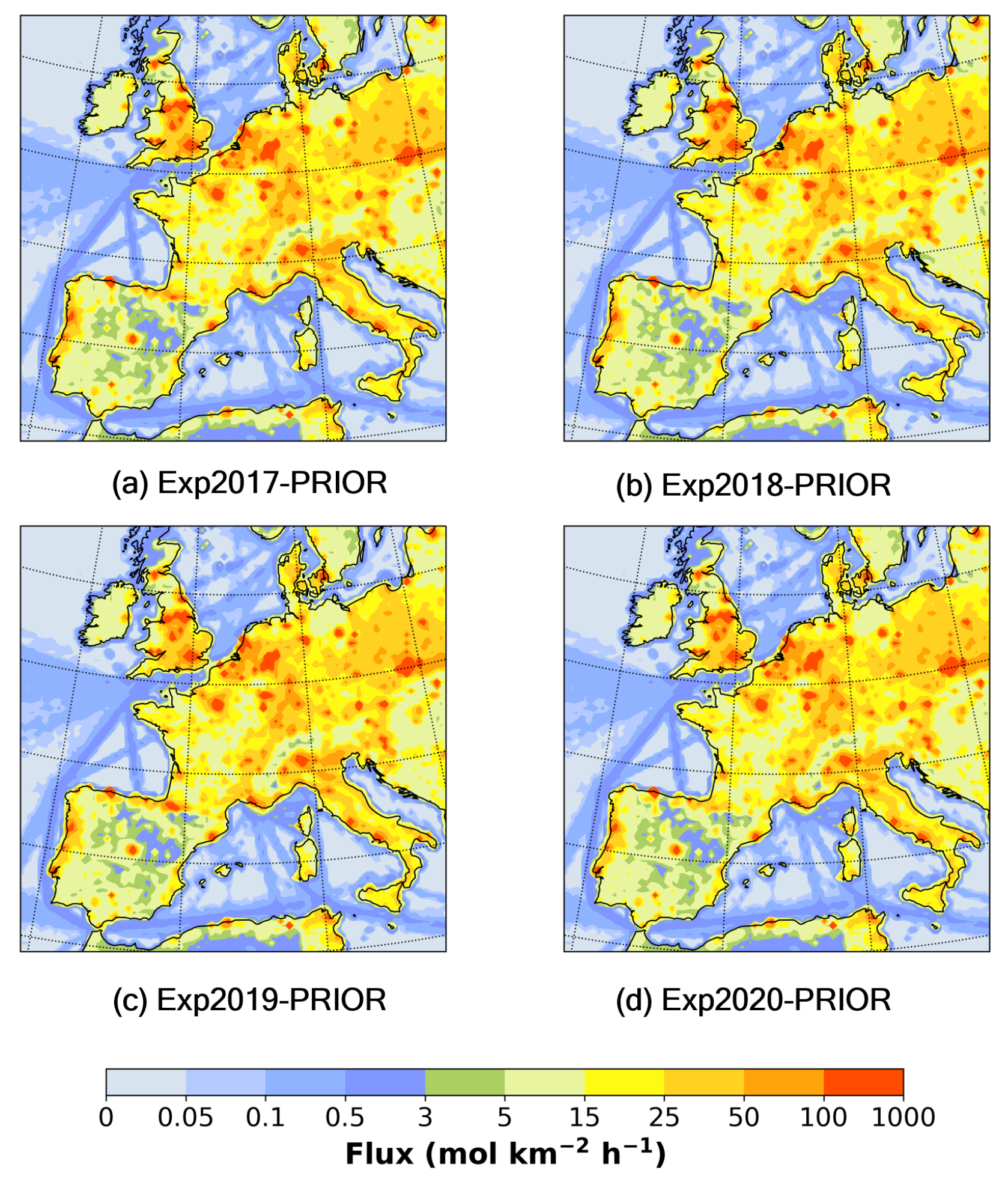
MOPITT, aboard NASA’s Terra satellite, is the first space-borne instrument to provide measurements of CO on a continuous basis since March 2000 [71]. MOPITT operates in a sun-synchronous orbit at an altitude of 705 km with an equator-crossing time at 10:30 a.m. local time. It has a swath width of 640 km, crossing the satellite track with a footprint size of 22 km × 22 km at nadir and can complete global measurement coverage every 3 days [71].
MOPITT measures CO in the 4.7- μ m TIR band and 2.3- μ m NIR band simultaneously. TIR radiances are most sensitive to CO in the middle and upper troposphere, whereas NIR observations mainly provide information about the CO total column with uniform sensitivity throughout the troposphere [72]. In the MOPITT CO data products, the retrieved CO profiles are expressed by a floating surface level and nine uniformly spaced levels from 900 hPa to 100 hPa [73]. Since data products Version 5 [72], MOPITT provides multi-spectral TIR/NIR joint retrieval CO products with greater sensitivity to CO in the lower troposphere [74], which can be used to invert surface-CO emissions [15,28,38].
In this research, MOPITT version 8 (V8) multi-spectral TIR/NIR CO retrieval data products (MOPV8J) [75,76] were used. Overall biases of MOPV8J [75,76] vary from about −5% at 600 hPa to about 7% at 200 hPa [77], and bias drift has been decreased to statistically negligible values (0.1% yr 1 or less) at all retrieval levels [77]. A recent study comparing MOPITT V8 CO retrieval products [75,76] with aircraft profiles (including in the winter) also showed that MOPITT generally agrees reasonably well with in situ profiles over both urban and non-urban regions, with biases ranging from −0.7% to 0.0% [78].
Figure 2 shows the average of the averaging kernel row sums of CO retrievals over the domain (shown by Figure 1) in four consecutive winter seasons (i.e., December–February) from 2017 to 2020 in MOPV8J [75,76]. The mean averaging kernel row sums of the surface level (1000 hPa in Figure 2) was about 0.25. Table 2 shows the Mean Absolute Error (MAE), RMSE, and percentage of difference relative to a priori between CO retrievals and the corresponding a priori CO mixing ratios in MOPV8J. The a priori CO mixing ratios are based on climatological values form 2000 to 2009, simulated by the CAM-Chem model [75]. For each level, the greater the deviation of the retrieved value from the a priori ratios, the more information content the MOPITT observation provides [79]. In Table 2, the difference relative to the a priori ratio of the surface-level CO was 14.79%, which was similar to that of the other levels, suggesting that MOPITT’s surface-level observations contain roughly the same amount of information as the other levels.
In order to compare vertical CO concentration profiles modeled by the CO flux inversion system with MOPITT CO retrievals, the modeled CO concentration profiles need to be converted by an observation operator F defined as [37]:
F ( x ) = y a + A ( H ( x ) y a ) ,
where A is the averaging kernel of the MOPITT retrieval, H ( x ) and y a are the modeled CO concentration profile interpolated to the vertical levels of the MOPITT retrieval and the prior CO profile of the MOPITT retrieval, respectively. Both A and y a are provided in MOPV8J for each CO retrieval [75].

2.2.2. Prior Fluxes

Anthropogenic, biogenic, and biomass-burning fluxes constituted the prior fluxes of the regional CO flux inversion system.
The anthropogenic fluxes were from the Emissions Database for Global Atmospheric Research (EDGAR) V4.3.2 part II Air Pollutants gridmaps dataset [80,81]. The EDGAR V4.3.2 part II dataset provides global emission gridmaps of CO and other air pollutants caused by all anthropogenic activities, except large-scale biomass burning, land use, land-use change, and forestry from 1970 to 2012 [34].
The biogenic fluxes were calculated by the Model of Emissions of Gases and Aerosols from Nature Version 2.1 (MEGAN V2.1) [82], which is coupled within the WRF-Chem model [49,50]. The input data files [83] needed by MEGAN V2.1 [82] were downloaded from the University Corporation for Atmospheric Research (UCAR). MEGAN V2.1 is a global modeling system for estimating the net emission of gases and aerosols from terrestrial ecosystems into the atmosphere at a spatial resolution of 1 km or less [82].
The biomass-burning fluxes were from the Fire Inventory from NCAR Version 1.5 (FINN V1.5) dataset [17,84]. The FINN V1.5 dataset provides global daily open biomass-burning emission estimates at a spatial resolution of 1 km or less based on the framework described by Wiedinmyer [17,85].

2.2.3. Chemical Initial and Boundary Conditions

The CAM-chem dateset [48,86] provided the concentration constraints of CO and 35 other gases, including atmospheric sources and sinks of CO, as the initial and boundary conditions of the regional CO flux inversion system, respectively. The spatial and temporal resolution of the CAM-chem outputs [86] are 0.9 ° × 1.25 ° and 6 h, respectively. The CAM-Chem [87] model is a component of the NCAR Community Earth System Model (CESM) [88]. The “Chemistry” in CAM-Chem is based on the Model for Ozone and Related chemical Tracers (MOZART) [52] family of chemical mechanisms, with various choices of complexity for simulations of global tropospheric and stratospheric atmospheric compositions [89].

2.2.4. Meteorological Data

The Final Operational Global Analysis data (FNL) with 1 ° × 1 ° spatial resolution and 6-h interval from the National Centers for Environmental Prediction (NCEP) [90,91] were used as meteorological initial and boundary conditions of the regional CO flux inversion system.
The NCEP ADP Global Upper Air and Surface Weather Observations [92,93], which are composed of a global set of surface and upper-air reports operationally collected by NCEP, were used as meteorological observations in this research. The meteorological observations from a total of 71 World Meteorological Organization (WMO) meteorological stations were used in this research. Their locations are shown in Figure S4.

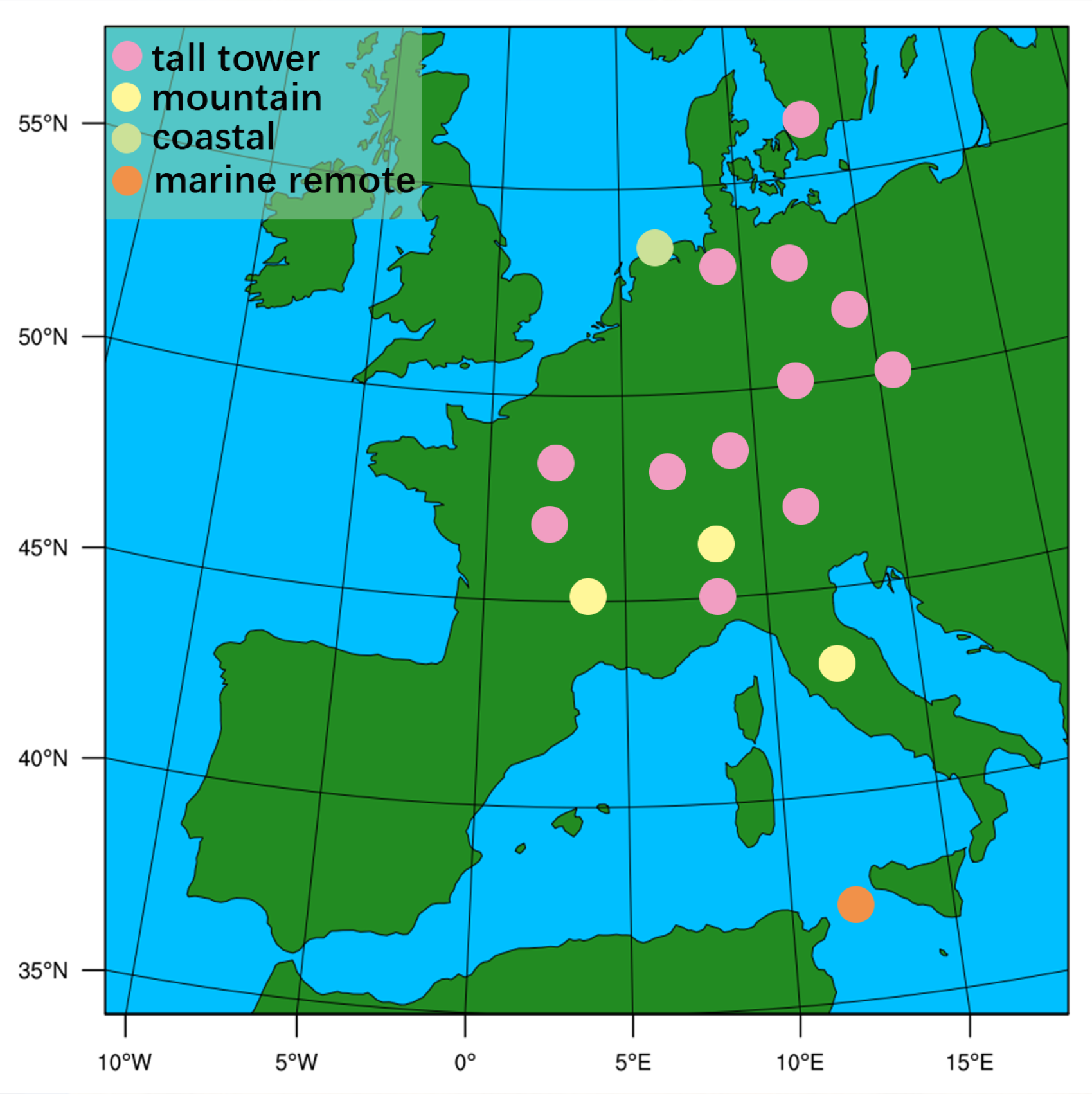
2.2.5. ICOS CO Observations

The ICOS consists of a network of atmosphere stations that carry out standardized, high-precision, and long-term monitoring of atmospheric greenhouse gases in 13 European countries [47]. Atmospheric measurements are usually taken on top of tall towers, in mountainous terrain, or in remote environments. These sites are usually not influenced much by local phenomena, but are rather exposed to atmospheric transport and processes covering larger areas. A site chosen for installing an atmosphere station will typically be representative of a footprint area of more than 10,000 km 2 [94]. The hourly averaged CO concentrations after a final quality control [95] of 17 atmosphere stations from ICOS [47] Atmosphere Release 2021-1 of Level 2 Greenhouse Gas Mole Fractions data product [94,96] were used in this research to evaluate the assimilation results of CO concentrations over western Europe. These 17 ICOS atmosphere stations are divided into four types, i.e., type of mountain, tall tower, marine remote, and coastal. Their locations are shown in Figure 1 and their detailed information is listed in Table S1.

2.3. Experiment Design

2.3.1. Study Area and Periods

As shown in Figure 1, western Europe was chosen as the study area because: (1) western Europe is a highly industrialized region in which anthropogenic CO emissions account for the majority of surface-CO fluxes, and biogenic CO fluxes from the ecosystem in the winter season will not change much in a short period of several years, as shown in Table 3; (2) western Europe has a well-developed and organized statistical infrastructure that enables it to have quite accurate emission inventories with uncertainty of less than 5% [42]; (3) all western European countries are Annex I countries [97], and the annual national emissions inventories they submitted to the UNFCCC can be used to evaluate the CO flux inversion results, and (4) there are relatively abundant ground-based CO observations available for evaluation.
Four consecutive winter seasons (i.e., December–February) from 2017 to 2020 were selected as the study periods because: in Europe, in the wintertime, the CO concentrations and anthropogenic CO emissions are at the highest level [38,43] and ecosystem activities are at the lowest levels, which means biogenic CO emissions and biogenic atmospheric sources of CO, such as CH 4 and NMVOC, are at their lowest levels in a year. Furthermore, wildfire and biomass-burning CO emissions are also at their lowest levels during this period of a year [44,45]. Therefore, according to the prior CO fluxes shown in Table 3, it was assumed that the anthropogenic CO emissions accounted for the super majority of the winter CO fluxes in western Europe. Based on this assumption, emission inventories submitted to the UNFCCC [46] by western European countries were used to evaluate the accuracy of winter CO fluxes inverted by the inversion system.

2.3.2. Experiment Setting

Four sets of experiments, namely, Exp2017, Exp2018, Exp2019, and Exp2020, were carried out to evaluate the CO flux, XCO, and surface-CO concentrations over western Europe in four consecutive winter seasons since 2017. Each set of experiments consisted of three parallel experiments of DA, SIM, and SIM_anthro.
The DA experiments inverted the posterior CO fluxes by assimilating MOPITT observations on the basis of the prior CO fluxes. The final CO concentration results of the DA experiments were generated by applying the posterior CO fluxes to the WRF-Chem model once again and without the assimilation, similar to the approach used in the CarbonTracker [98]. The SIM and SIM_anthro experiments used the prior CO fluxes and the prior anthropogenic CO fluxes to simulate the CO concentrations by the WRF-Chem model under the same experimental conditions as the DA experiments, respectively. There was no assimilation process in the SIM and SIM_anthro experiments.
The duration of each experiment was from 1 December to 28 February of the following year. The spin-up phase of each DA experiments occured two weeks before 1 December. The simulation cycle was 6-h at 00:00, 06:00, 12:00, and 18:00 UTC, respectively, and the advancing time step was 150 s.
The size of ensemble members of the DA experiments was set to 20, the same as in [65,66,99]. A three-dimensional Gaspari–Cohn localization function [100] with a horizontal half-width of 0.1 radian and a vertical half-width of 200 hPa was used to compensate the under-sampling errors caused by the limited size of ensemble members, according to [101].

2.3.3. Experiment Inputs

The initial and boundary chemical conditions of the ensemble members were generated by imposing zero mean perturbations following Gaussian distributions to gas concentrations extracted from the CAM-Chem dateset [48]. The standard deviation of these Gaussian perturbations were 30% of the standard deviations of the gas concentrations calculated from the CAM-Chem dataset [48]. The prior anthropogenic and biomass-burning fluxes were interpolated from the EDGAR V4.3.2 dataset [80] and FINN V1.5 dataset [17] by the existing WRF-Chem preprocessor tools [102] provided by the Atmospheric Chemistry Observations and Modeling Lab of NCAR. The latest available monthly anthropogenic CO emissions provided by EDGAR V4.3.2 [80] are from 2010; therefore, the same prior anthropogenic CO emissions were used in all four experiments. The prior biogenic fluxes were generated by MEGAN V2.1 [82] with the input files [83] downloaded from UCAR. The prior oceanic source of CO fluxes was not considered in this study, because they are considered to be very small compared to the anthropogenic emissions [19]. The prior CO fluxes for each experiment are listed in Table 3 and their distributions are shown in Figure 3. The prior CO fluxes of ensemble members were generated by a method similar to that of the chemical condition ensembles.
The mean retrieved surface-level CO concentrations and XCO retrievals from MOPV8J [75,76], assimilated in the four experiments, are shown in Figure 4.
The initial and boundary meteorological conditions of ensemble members were generated by WRF variational data assimilation (WRFDA) [103] with the configure option of “cv_options = 3”, the same as that used in Zhang’s studies [40,64].

2.3.4. Evaluation Metrics

The experimental results of the CO concentrations were evaluated by the ground-CO observations from ICOS [47] and the external CAM-Chem results [48] corresponding to the experiments. The distributions of mean surface CO concentrations and XCO extracted from the external CAM-Chem results [48] corresponding to the four experiments are shown in Figure 5.
The CO concentration results of the nearest four grid cells around an ICOS site [47] were first interpolated to the location of the site and then interpolated to the same pressure level or the same altitude of the site before evaluation. The consistency between the final interpolated CO concentration result and the corresponding ICOS observation value [47] was evaluated by means of MBE, RMSE, and the correlation coefficient (CORR). They were defined in the same way as the Equations (6), (8), and (9) in Zhang’s work [64].

3. Results and Discussion

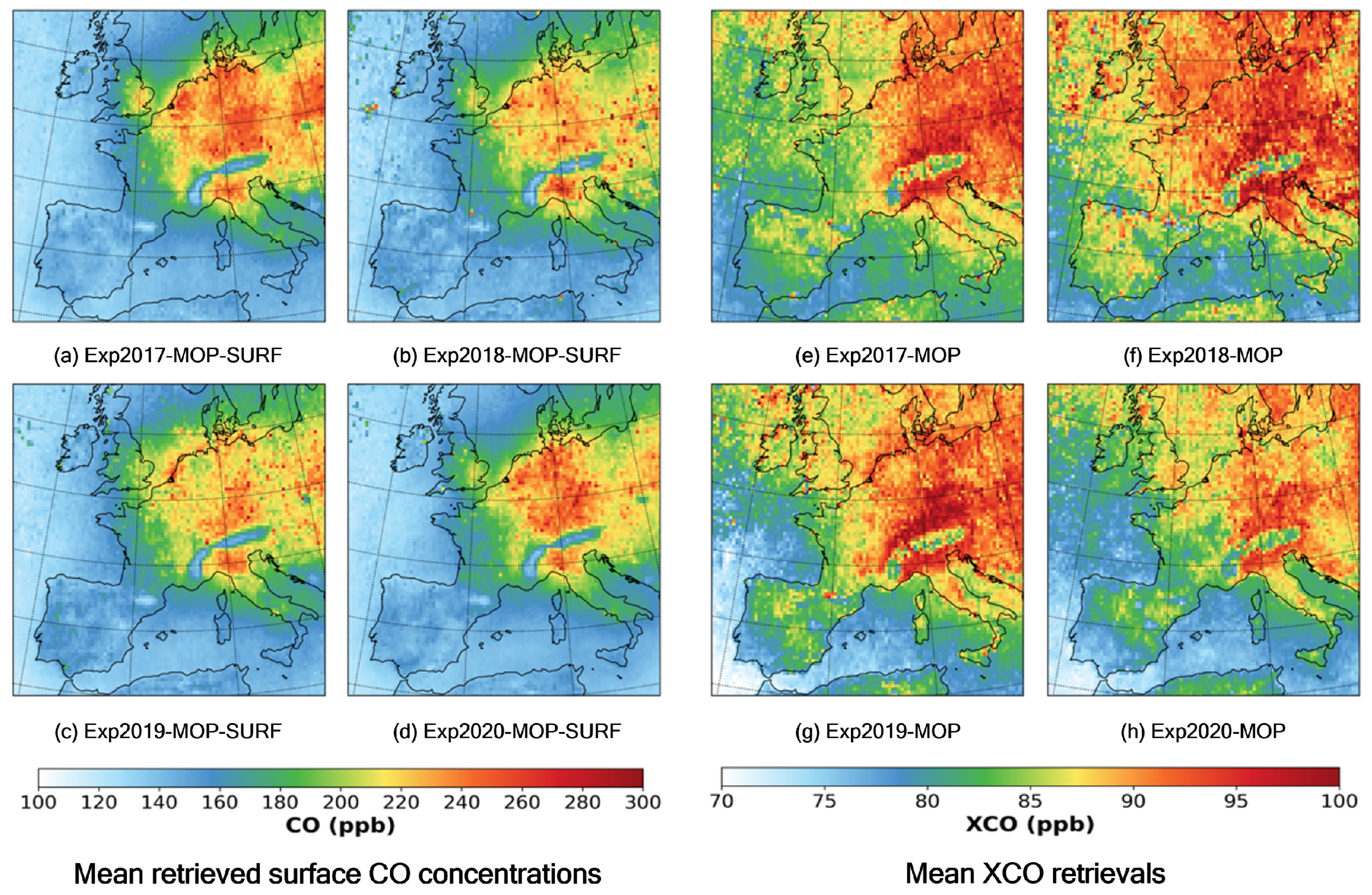
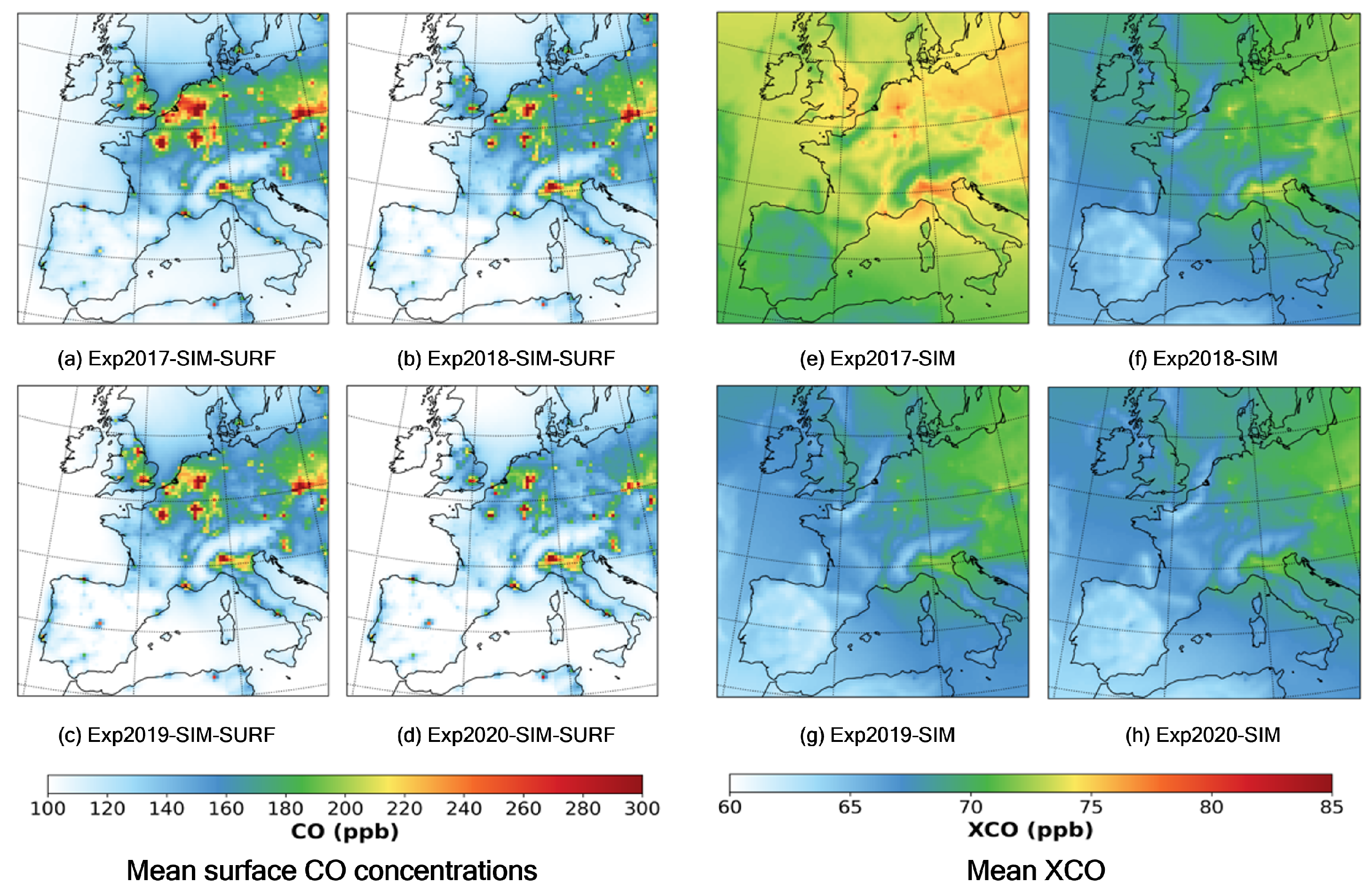
3.1. CO Concentration Experimental Results

The mean surface-CO concentrations (MSCC) and XCO distributions of the DA and SIM experimental results are shown in Figure 6 and Figure 7, respectively.
The MSCC and XCO of the four consecutive winter seasons in western Europe from 2017 to 2020 estimated by the DA, SIM, and SIM_anthro experiments are listed in Table 4 and Table 5, respectively. The MSCC and XCO of the same periods in western Europe, extracted from MOPV8J [75,76] and the external CAM-Chem results [48], are also listed in the tables for reference. The CO concentrations and XCO extracted from the external CAM-Chem results were not used in all the experiments.
As shown in Table 4 and Table 5, the average differences of MSCC and XCO between the DA experiments and the MOPV8J data [75,76] were −28.92 ppb and −12.82 ppb, which were 1.09-ppb and 13.87-ppb better than those of between the SIM experiments and the MOPV8J data [75,76]. This was as expected; since the MOPV8J data were assimilated in the DA experiments, the DA experimental results should be closer to the MOPV8J data [75,76] than the SIM results. The differences between the DA, the SIM experimental results, and the MOPV8J data are shown in Figure 8 and Figure 9, respectively. The comparison of surface-CO concentrations and XCO of the experimental results with the MOPV8J data [75,76] are listed in Tables S2 and S3, respectively. The differences between the DA and SIM experimental results are shown in Figure S1.
From the MSCC of the SIM experimental results, shown in Figure 7, and the differences of the MSCC between the SIM experiments and the MOPV8J data [75,76], shown in Figure 9, the locations of London, Paris, Berlin, Rotterdam, Antwerp, Madrid, Rome, Naples, and other major western European cities can be clearly identified. From the same results and differences of the DA experiments shown in Figure 6 and Figure 8, not only the above major cities can be identified, but also the urban agglomerations composed of cities in the Netherlands and Belgium, northern Italy, etc., are more clearly reflected.
As shown in Figure 7, the MSCC distributions of the SIM experimental results were roughly similar; so were the differences of the MSCC between the SIM experiments and the MOPV8J data [75,76], as shown in Figure 9.
However, for the DA experiments, as shown in Figure 6 and Figure 8, the MSCC distribution, the difference of MSCC relative to the MOPV8J data [75,76], in the winter of 2017 were significantly different from those in the winter of the other three years. The DA experimental results for the winter season of 2017 showed high MSCC across a large region where Germany, the Czech Republic, Hungary, Poland, and other countries were located. Furthermore, as shown in Figure 6 and Figure 7, both the DA and SIM experiments showed that the same region also had high mean XCO in the winter of 2017, making the mean XCO distribution results of the DA and SIM experiments for the winter season of 2017 significantly different from those in the other three years.
The MSCC and XCO of the SIM experimental results depended on the prior CO fluxes and the initial and boundary conditions. As shown in Table 3, the maximum difference between the four prior CO fluxes was 2.86%. There were also no large differences between the prior CO flux distributions of the four winter seasons, as shown in Figure 3. Table 4 and Table 5 also confirmed that there were no large differences between the MSCC and XCO of the MOPITT data over the four winter seasons. Therefore, the significant differences between the SIM experimental results for the winter season of 2017 and those for the other three winter seasons were likely due to the differences of the initial and boundary conditions. Actually, from the MSCC and XCO distributions of the external CAM-Chem results [48] shown in Figure 5, it is clear that the mean XCO distributions for the winter of 2017 were significantly different from those for the other three winter seasons, and the MSCC and mean XCO of the external CAM-Chem results [48], listed in Table 4 and Table 5, also confirmed this significant difference. Although the external CAM-Chem results [48] were not used in all the experiments, they were derived from the same dataset as the initial and boundary conditions; therefore, there were strong correlations between them.
Similarly, there were no significant differences between the MSCC and mean XCO distributions of the MOPV8J data [75,76] of the four winter seasons, as shown in Figure 4, and Table 4 and Table 5 also confirmed that there were no large differences between the MSCC and XCO of the MOPITT data over the four winter seasons. Therefore, the significant differences between the DA experimental results for the winter season of 2017 and those for the other three winter seasons were also likely due to the differences of the boundary conditions.
The MSCC and XCO results of the SIM_anthro experiments are shown in Figure 10. Since the only difference between the SIM and SIM_anthro experiments was that the prior CO fluxes for the SIM experiments were the sum of the prior anthropogenic, biogenic, and biomass-burning CO fluxes listed in Table 3, those for the SIM_anthro experiments were only the prior anthropogenic CO fluxes. Furthermore, the differences between the prior CO fluxes of the SIM and SIM_anthro experiments were less than 5.37%, as shown in Table 3. Therefore, it was not surprising that the results of the two experiments were close to each other; the differences of the MSCC and mean XCO results between the two experimental results were no more than than 0.97 ppb and 0.1 ppb, respectively. The differences between the SIM and SIM_anthro experimental results are shown in Figure S2.

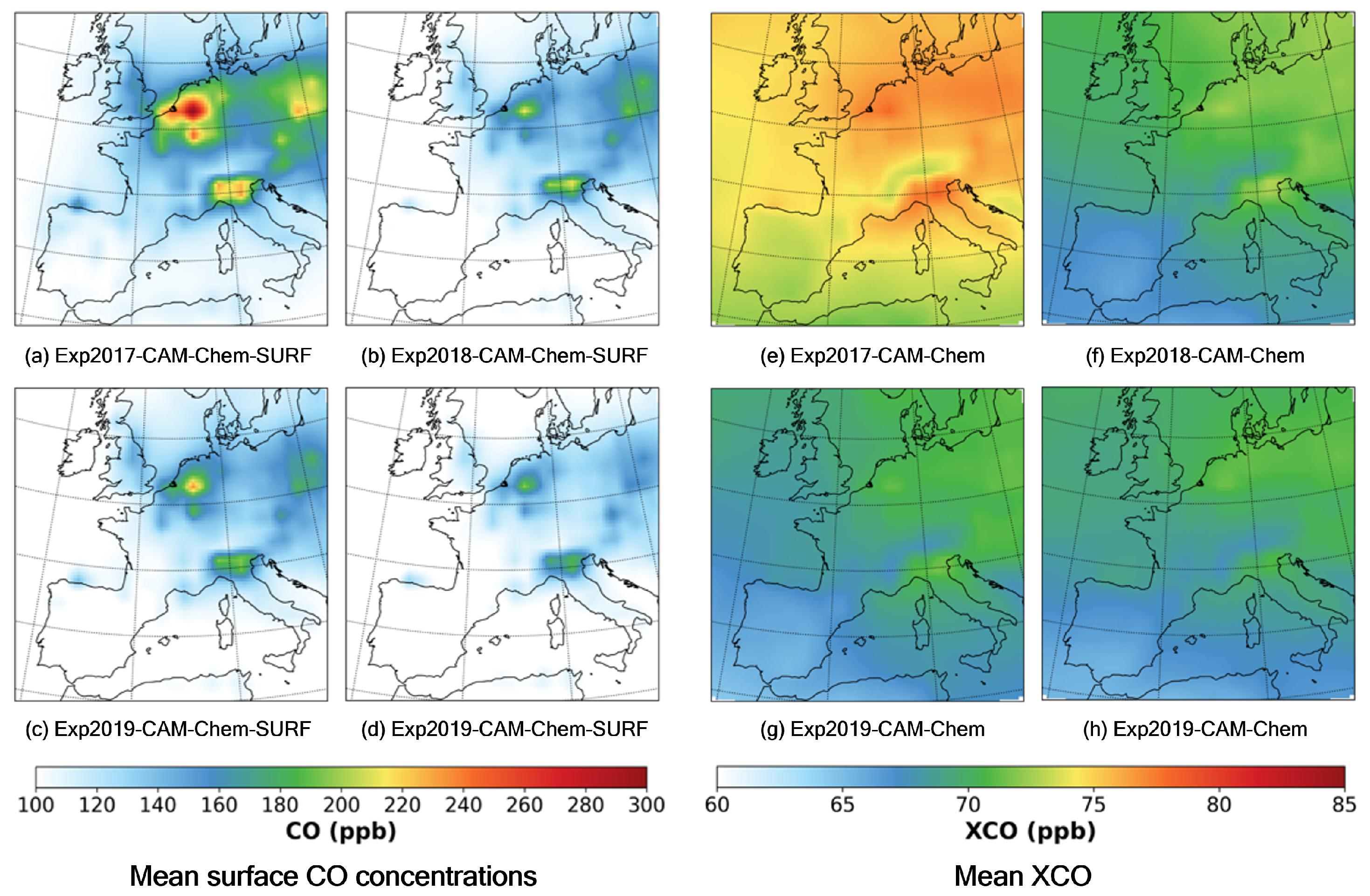
3.1.1. Evaluated by the External CAM-Chem Results

The differences of the MSCC and XCO between the DA, SIM experiments, and the external CAM-Chem results are shown in Figure 11 and Figure 12, respectively. Comparing Figure 11 and Figure 12, the effects of assimilating the MOPV8J data on the MSCC and the mean XCO results of the DA experiments can be clearly seen. The differences of the MSCC and XCO between the MOPV8J data [75,76] and the external CAM-Chem results [48] are shown in Figure S3.
The MBE and RMSE of the MSCC and mean XCO for the DA, SIM experiments, and the MOPV8J data [75,76], relative to the external CAM-Chem results, [48] are listed in Table 6 and Table 7, respectively. The MBE between the posterior XCO, estimated by the four DA experiments, and the CAM-Chem results [48] were 0.38 ppb, 0.86 ppb, −0.43 ppb, and −0.59 ppb, respectively. The DA experimental results were, on average, 0.05-ppb higher than those of the external CAM-Chem results in the four-year experiments. The MBE between the posterior surface-CO concentrations, estimated by the four DA experiments and the CAM-Chem results [48], were 33.84 ppb, 20.06 ppb, 14.71 ppb, and 14.53 ppb, respectively. The surface-CO concentrations of the DA experiments were, on average, 20.79-ppb higher than those of the external CAM-Chem results [48].
In the SIM experiments with the same initial and boundary conditions as the DA experiments, all the mean winter seasonal XCO, simulated by the WRF-Chem model and using the prior CO fluxes listed in Table 3, were lower than those mean posterior XCO results of the DA experiments, and also lower than those from the external CAM-Chem results [48]. During the four-year experiments, the Sim experimental XCO results were 2.11-ppb, 1.24-ppb, 0.57-ppb, and 0.45-ppb lower than those of the DA experiments, and were 1.73-ppb, 0.38-ppb, 1.00-ppb, and 1.04-ppb lower than those from the external CAM-Chem results [48], respectively. This fact implied that the prior CO fluxes used in the DA and SIM experiments might underestimate the actual CO flux values in the winter months. Actually, the annual anthropogenic CO emissions of western Europe in 2010, provided by EDGAR V5.0 [104], is 38.15% higher than that provided by EDGAR V4.3.2 [80].

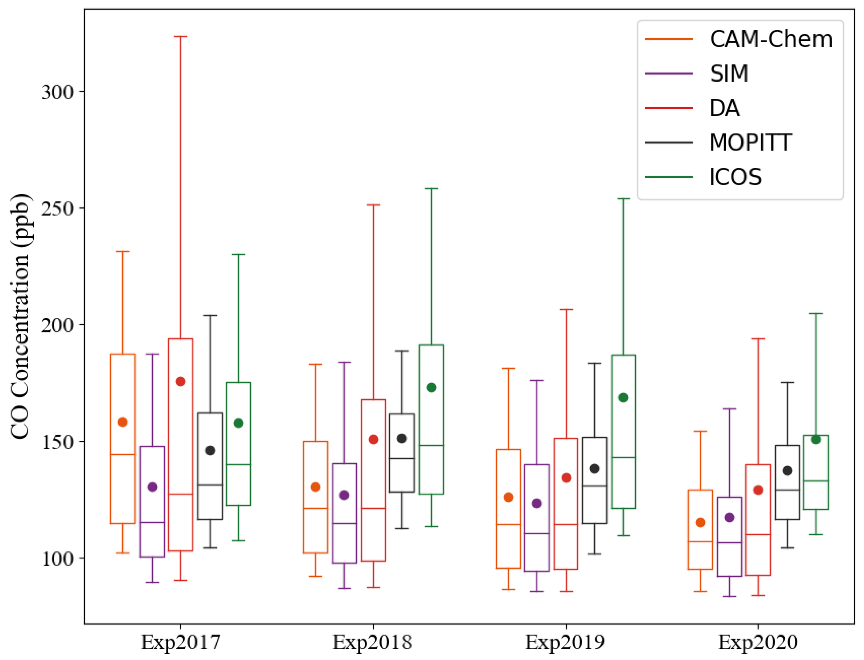
3.1.2. Evaluated by the ICOS CO Observations

The number of the ICOS CO observations used in the evaluation are listed in Table 8. The CO concentrations measured at the highest observation point of the tall tower stations, which are considered closer to the background, were chosen to evaluate the experimental results. The boxplots of the DA, SIM experimental results, and CO concentrations from the external CAM-Chem results [48], and the MOPV8J data [75,76] compared with the ICOS CO observations [47] are shown in Figure 13. The DA and SIM experimental results, the external CAM-Chem results [48], and the MOPV8J data [75,76] were interpolated to the same location and the same pressure level or the same altitude of the ICOS observations [47] before evaluation. The mean and median CO concentration values in the boxplots are listed in Table 9.
As can be seen from Table 9, the mean and median CO concentrations observed by the ICOS sites [47] in the winter of 2018 increased by 15.13 ppb and 8.30 ppb, respectively, compared to the same period in 2017. After this significant increase, the mean and median of ICOS CO concentration observations [47] had maintained a downward trend between the consecutive winter seasons of the following years. The variation trend in the external CAM-Chem results [48] was a straight downward trend. Compared with 2017, the mean and median CO concentrations from the external CAM-Chem results [48] in the winter of 2018 decreased significantly, by 27.93 ppb and 23.06 ppb, respectively. The comparison of these two trends suggested that the boundary conditions provided by the CAM-Chem datasets might be high in 2017.
The evaluation results between the ICOS observations [47] and CO concentrations from the DA, SIM experiments, and the external CAM-Chem results [48] are listed in Table 10. All the MBE values were negative, implying that the CO concentrations from the DA experiments and the external CAM-Chem results [48] were, overall, lower than the ICOS observations [47], which is consistent with Lamarque’s research [87]. The average MBE of the DA experiments was −22.43 ppb, and was 17.52-ppb and 14.84-ppb better than that of the SIM experiments and the external CAM-chem results [48], respectively. The RMSEs of the DA experiments were also the best, the average RMSE was 4.17-ppb and 13.03-ppb better than that of the SIM experiments and the external CAM-chem results [48], respectively.

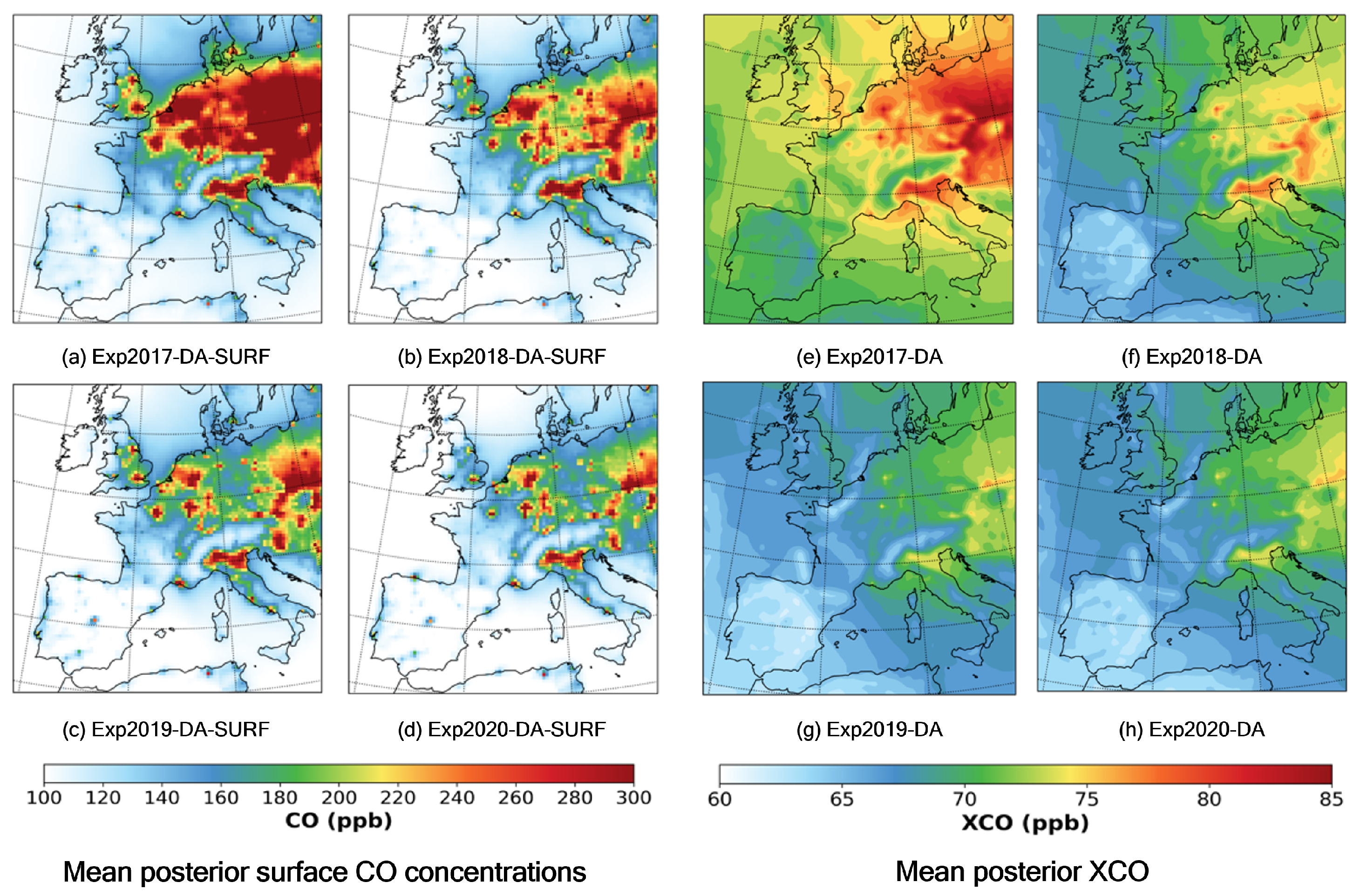
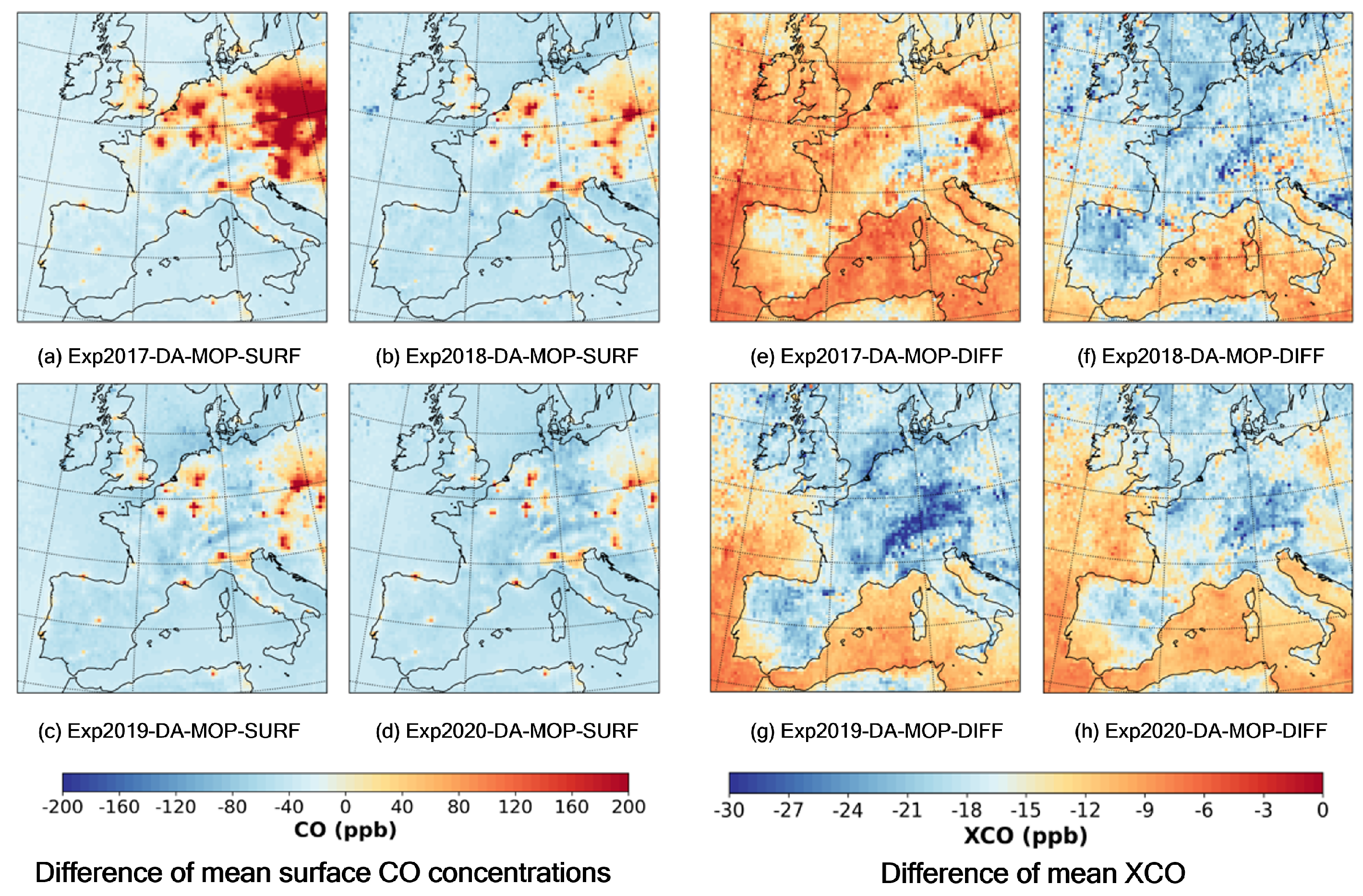
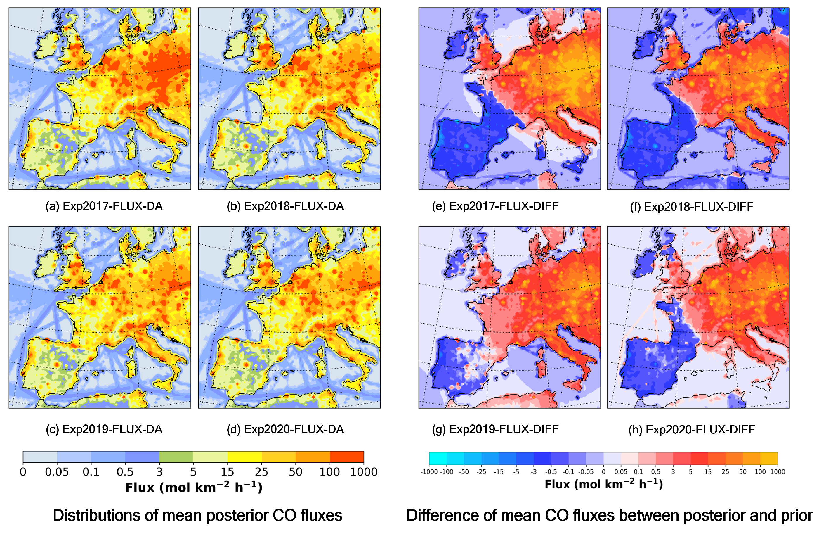
3.2. CO Flux Inversion Results

The mean posterior CO fluxes inverted by the DA experiments are listed in Table 11. Their distributions and their differences relative to the prior CO fluxes are shown in Figure 14. The mean posterior CO fluxes of the four consecutive winter seasons in western Europe from 2017 to 2020 were 28.45 mol km 2 h 1 , 21.79 mol km 2 h 1 , 20.19 mol km 2 h 1 , and 19.86 mol km 2 h 1 , which increased by 13.90 mol km 2 h 1 (95.53%), 7.48 mol km 2 h 1 (52.27%), 5.47mol km 2 h 1 (37.16%), and 5.37 mol km 2 h 1 (37.06%), compared with the prior CO fluxes, respectively. The difference percentage between the posterior and prior fluxes of 2017 was as high as 95.53%, which was significantly larger than that of the other three years. This unusually high difference in 2017 was thought to be caused by the high boundary conditions discussed earlier. As shown in Figure 14, in the distribution of differences between the posterior and prior fluxes, the areas with significant increases in fluxes roughly coincided with the high XCO areas of the MOPV8J data [75,76], as shown in Figure 4.

3.3. Compared with the UNFCCC Inventories

The comparison results of the winter CO fluxes of 15 western European countries inverted by the DA experiments and the corresponding anthropogenic CO emissions extracted from the UNFCCC inventories [46] are listed in Table 12. Figure S5 shows the map of these 15 countries. Up to now, the latest CO emission inventories available from the UNFCCC [46] are for 2019. Using the methodology described by Crippa [43], the winter seasonal anthropogenic CO emissions of these 15 countries from 2017 to 2019 were extracted from their national inventories submitted to the UNFCCC [46]. Table 12 indicates that the CO emissions inverted by the DA experiments roughly match the anthropogenic CO emissions extracted from the UNFCCC inventories. The differences between them were 13.36%, −4.59%, and −4.76% during the winter seasons from 2017 to 2019, respectively. As expected, the difference of 2017 was much larger than that of the other 2 years. Given the high boundary conditions discussed earlier, a 13.36% difference for 2017 was not too bad.
The comparisons with the UNFCCC inventories [46] confirmed that the assumption in the experimental design, i.e., that the super majority of CO emissions in the winter season in western Europe was caused by anthropogenic emissions, was reasonable.

4. Conclusions

In this study, the CO fluxes and concentrations of the four consecutive winter seasons in western Europe from 2017 to 2020 were estimated through the assimilation of the MOPV8J data [75,76] by a regional CO flux inversion system.
The analyses of the MOPV8J data used by the inversion system indicated that the mean averaging kernel row sums of the surface level was about 0.25, and the difference percentage of the surface-level retrievals relative to a priori CO-mixing ratios was 14.79%, which was similar to that of the other levels.
The inverted CO fluxes of the four winter seasons were 6198.15 kilotons, 4939.72 kilotons, 4697.80 kilotons, and 5456.19 kilotons, respectively. Compared with the prior CO fluxes, the inverted CO fluxes of the four winter seasons increased by 95.53%, 52.27%, 37.16%, and 37.06%, respectively.
Based on the assumption that the anthropogenic CO emissions accounted for the super majority of the winter CO fluxes in western Europe, the UNFCCC inventories [46] were used to evaluate the accuracy of the above inverted CO fluxes. The evaluation results indicate that the differences between the inverted CO fluxes and UNFCCC inventories [46] of the three winter seasons of 2017 to 2019 were 13.36%, −4.59%, and −4.76%, respectively. Considering the influence of boundary conditions on the uncertainty of the CO fluxes’ inversion results, the evaluation results suggested that the above assumption was reasonable.
Detailed surface-CO concentrations and XCO comparative analyses between the DA and SIM experimental results, the external CAM-Chem results [48], and the MOPV8J data [75,76] were conducted. The comparative analysis results indicated that the DA and SIM experimental results of 2017 were obviously affected by the high boundary conditions.
The CO concentrations results of the experiments were also evaluated by the ICOS CO concentration observations [47]. The evaluation results showed that the average MBEs and RMSEs of the DA experiments were better than those of the SIM experiments and the external CAM-Chem results [48]. The average MBE of the DA experiments was −22.43 ppb, and was 17.52-ppb and 14.84-ppb better than that of the SIM experiments and the external CAM-chem results [48], respectively. The average RMSE was 4.17-ppb and 13.03-ppb better than that of the SIM experiments and the external CAM-chem results [48], respectively. The comparison of the ICOS data [47] with the external CAM-Chem results [48] also confirms that the boundary conditions might be high in 2017.

Supplementary Materials

The following supporting information can be downloaded at: https://www.mdpi.com/article/10.3390/rs14051133/s1, Figure S1: Difference of the mean surface CO concentrations and XCO between the DA and SIM experimental results (DA minus SIM); Figure S2: Difference of the mean surface CO concentrations and XCO between the SIM and SIM_anthro experiments (SIM minus SIM_anthro); Figure S3: Difference of the mean surface CO concentrations and XCO between the MOPITT data and the external CAM-Chem datasets (MOPITT minus CAM-Chem); Figure S4: Location of 71 WMO meteorological stations; Figure S5: Map of the 15 Western European countries; Table S1: Information of the ICOS stations used in this study; Table S2: Comparisons of the surface CO concentrations with the MOPPIT data; Table S3: Comparisons of the XCO with the MOPPIT data.

Author Contributions

Conceptualization, Q.G. and Y.H.; methodology, Y.H., J.W. and Q.G.; software, Y.H. and J.J.; validation, Y.H., J.J. and Q.G.; formal analysis, Y.H., Q.G. and J.J.; investigation, Y.H. and Q.G.; resources, J.W.; data curation, Y.H., J.J. and Z.Z.; writing—original draft preparation, Y.H. and Q.G.; writing—review and editing, Q.G. and J.W.; visualization, Y.H., J.J. and Z.Z.; supervision, Q.G. and J.W. All authors have read and agreed to the published version of the manuscript.

Funding

This research was funded by the Key Research Program of the Chinese Academy of Sciences (ZDRW-ZS-2019-1), the International Partnership Program of the Chinese Academy of Sciences (131211KYSB20180002), and the Chinese Academy of Sciences Youth Innovation Promotion Association Funding (2018327).

Institutional Review Board Statement

Not applicable.

Informed Consent Statement

Not applicable.

Data Availability Statement

The CO concentration and flux data generated and used by this study are openly available in: https://github.com/hgrhgy/remote_sensing_2022_CO_FLUX_EU, accessed on 24 February 2022.

Acknowledgments

The authors acknowledge the free availability of the WRF-Chem model [49,50] provided by NOAA Earth System Research Laboratories, the WRF-Chem preprocess tools [102], the DART system [63], and the Community Atmosphere Model with Chemistry (CAM-Chem) Outputs as Boundary Conditions dataset [86] provided by NCAR, the MOPITT version 8 level 2 CO retrieval data products [76] from NASA Earthdata center, the Final Operational Global Analysis data (FNL) [91] and Global Upper Air and Surface Weather Observations [93] from NCEP, ground-CO concentration observations from ICOS [94], the anthropogenic CO fluxes from the Emissions Database for Global Atmospheric Research part II Air Pollutants gridmaps dataset V4.3.2 [81] and V5.0 [104] and UNFCCC National Inventory Submissions 2021 [46], the input data files [83] needed to calculate the biogenic CO fluxes from the University Corporation for Atmospheric Research, and the biomass-burning CO fluxes from the Fire Inventory from NCAR V1.5 dataset [84].

Conflicts of Interest

The authors declare no conflict of interest.

References

  1. Myhre, G.; Shindell, D.; Bréon, F.; Collins, W.; Fuglestvedt, J.; Huang, J.; Koch, D.; Lamarque, J.; Lee, D.; Mendoza, B.; et al. Climate change 2013: The physical science basis. In Contribution of Working Group I to the Fifth Assessment Report of the Intergovernmental Panel on Climate Change; Cambridge University Press: Cambridge, UK, 2013; pp. 659–740. Available online: https://www.ipcc.ch/report/ar5/wg1/ (accessed on 21 November 2021).
  2. Turnbull, J.C.; Miller, J.B.; Lehman, S.J.; Tans, P.P.; Sparks, R.J.; Southon, J. Comparison of 14CO2, CO, and SF6 as tracers for recently added fossil fuel CO2 in the atmosphere and implications for biological CO2 exchange. Geophys. Res. Lett. 2006, 33. [Google Scholar] [CrossRef]
  3. Levin, I.; Karstens, U. Inferring high-resolution fossil fuel CO2 records at continental sites from combined 14CO2 and CO observations. Tellus B 2007, 59, 245–250. [Google Scholar] [CrossRef]
  4. Super, I.; Denier van der Gon, H.; Visschedijk, A.; Moerman, M.; Chen, H.; van der Molen, M.; Peters, W. Interpreting continuous in-situ observations of carbon dioxide and carbon monoxide in the urban port area of Rotterdam. Atmos. Pollut. Res. 2017, 8, 174–187. [Google Scholar] [CrossRef]
  5. Hoesly, R.M.; Smith, S.J.; Feng, L.; Klimont, Z.; Janssens-Maenhout, G.; Pitkanen, T.; Seibert, J.J.; Vu, L.; Andres, R.J.; Bolt, R.M.; et al. Historical (1750–2014) anthropogenic emissions of reactive gases and aerosols from the Community Emissions Data System (CEDS). Geosci. Model Dev. 2018, 11, 369–408. [Google Scholar] [CrossRef] [Green Version]
  6. Shindell, D.T.; Faluvegi, G.; Stevenson, D.S.; Krol, M.C.; Emmons, L.K.; Lamarque, J.F.; Pétron, G.; Dentener, F.J.; Ellingsen, K.; Schultz, M.G.; et al. Multimodel simulations of carbon monoxide: Comparison with observations and projected near-future changes. J. Geophys. Res. Atmos. 2006, 111. [Google Scholar] [CrossRef] [Green Version]
  7. Duncan, B.N.; Logan, J.A. Model analysis of the factors regulating the trends and variability of carbon monoxide between 1988 and 1997. Atmos. Chem. Phys. 2008, 8, 7389–7403. [Google Scholar] [CrossRef] [Green Version]
  8. Stein, O.; Schultz, M.G.; Bouarar, I.; Clark, H.; Huijnen, V.; Gaudel, A.; George, M.; Clerbaux, C. On the wintertime low bias of Northern Hemisphere carbon monoxide found in global model simulations. Atmos. Chem. Phys. 2014, 14, 9295–9316. [Google Scholar] [CrossRef] [Green Version]
  9. Logan, J.A.; Prather, M.J.; Wofsy, S.C.; McElroy, M.B. Tropospheric chemistry: A global perspective. J. Geophys. Res. Ocean. 1981, 86, 7210–7254. [Google Scholar] [CrossRef]
  10. Gaubert, B.; Worden, H.M.; Arellano, A.F.J.; Emmons, L.K.; Tilmes, S.; Barré, J.; Martinez Alonso, S.; Vitt, F.; Anderson, J.L.; Alkemade, F.; et al. Chemical Feedback From Decreasing Carbon Monoxide Emissions. Geophys. Res. Lett. 2017, 44, 9985–9995. [Google Scholar] [CrossRef] [Green Version]
  11. Taylor, J.A.; Zimmerman, P.R.; Erickson, D.J. A 3-D modelling study of the sources and sinks of atmospheric carbon monoxide. Ecol. Model. 1996, 88, 53–71. [Google Scholar] [CrossRef]
  12. Lelieveld, J.; Gromov, S.; Pozzer, A.; Taraborrelli, D. Global tropospheric hydroxyl distribution, budget and reactivity. Atmos. Chem. Phys. 2016, 16, 12477–12493. [Google Scholar] [CrossRef] [Green Version]
  13. Holloway, T.; Levy, H., II; Kasibhatla, P. Global distribution of carbon monoxide. J. Geophys. Res. Atmos. 2000, 105, 12123–12147. [Google Scholar] [CrossRef]
  14. Lamarque, J.F.; Bond, T.C.; Eyring, V.; Granier, C.; Heil, A.; Klimont, Z.; Lee, D.; Liousse, C.; Mieville, A.; Owen, B.; et al. Historical (1850–2000) gridded anthropogenic and biomass burning emissions of reactive gases and aerosols: Methodology and application. Atmos. Chem. Phys. 2010, 10, 7017–7039. [Google Scholar] [CrossRef] [Green Version]
  15. Zheng, B.; Chevallier, F.; Yin, Y.; Ciais, P.; Fortems-Cheiney, A.; Deeter, M.N.; Parker, R.J.; Wang, Y.; Worden, H.M.; Zhao, Y. Global atmospheric carbon monoxide budget 2000–2017 inferred from multi-species atmospheric inversions. Earth Syst. Sci. Data 2019, 11, 1411–1436. [Google Scholar] [CrossRef] [Green Version]
  16. Worden, H.M.; Bloom, A.A.; Worden, J.R.; Jiang, Z.; Marais, E.A.; Stavrakou, T.; Gaubert, B.; Lacey, F. New constraints on biogenic emissions using satellite-based estimates of carbon monoxide fluxes. Atmos. Chem. Phys. 2019, 19, 13569–13579. [Google Scholar] [CrossRef] [Green Version]
  17. Wiedinmyer, C.; Akagi, S.K.; Yokelson, R.J.; Emmons, L.K.; Al-Saadi, J.A.; Orlando, J.J.; Soja, A.J. The Fire INventory from NCAR (FINN): A high resolution global model to estimate the emissions from open burning. Geosci. Model Dev. 2011, 4, 625–641. [Google Scholar] [CrossRef] [Green Version]
  18. Van der Werf, G.R.; Randerson, J.T.; Giglio, L.; Collatz, G.J.; Kasibhatla, P.S.; Arellano, A.F., Jr. Interannual variability in global biomass burning emissions from 1997 to 2004. Atmos. Chem. Phys. 2006, 6, 3423–3441. [Google Scholar] [CrossRef] [Green Version]
  19. Conte, L.; Szopa, S.; Séférian, R.; Bopp, L. The oceanic cycle of carbon monoxide and its emissions to the atmosphere. Biogeosciences 2019, 16, 881–902. [Google Scholar] [CrossRef] [Green Version]
  20. Drummond, J.R.; Mand, G.S. The Measurements of Pollution in the Troposphere (MOPITT) Instrument: Overall Performance and Calibration Requirements. J. Atmos. Ocean. Technol. 1996, 13, 314–320. [Google Scholar] [CrossRef] [Green Version]
  21. Aumann, H.; Chahine, M.; Gautier, C.; Goldberg, M.; Kalnay, E.; McMillin, L.; Revercomb, H.; Rosenkranz, P.; Smith, W.; Staelin, D.; et al. AIRS/AMSU/HSB on the Aqua mission: Design, science objectives, data products, and processing systems. IEEE Trans. Geosci. Remote Sens. 2003, 41, 253–264. [Google Scholar] [CrossRef] [Green Version]
  22. Beer, R. TES on the aura mission: Scientific objectives, measurements, and analysis overview. IEEE Trans. Geosci. Remote Sens. 2006, 44, 1102–1105. [Google Scholar] [CrossRef]
  23. Clerbaux, C.; Boynard, A.; Clarisse, L.; George, M.; Hadji-Lazaro, J.; Herbin, H.; Hurtmans, D.; Pommier, M.; Razavi, A.; Turquety, S.; et al. Monitoring of atmospheric composition using the thermal infrared IASI/MetOp sounder. Atmos. Chem. Phys. 2009, 9, 6041–6054. [Google Scholar] [CrossRef] [Green Version]
  24. Veefkind, J.P.; Aben, I.; McMullan, K.; Förster, H.; de Vries, J.; Otter, G.; Claas, J.; Eskes, H.J.; de Haan, J.F.; Kleipool, Q.; et al. TROPOMI on the ESA Sentinel-5 Precursor: A GMES mission for global observations of the atmospheric composition for climate, air quality and ozone layer applications. RSE 2012, 120, 70–83. [Google Scholar] [CrossRef]
  25. Worden, H.M.; Deeter, M.N.; Frankenberg, C.; George, M.; Nichitiu, F.; Worden, J.; Aben, I.; Bowman, K.W.; Clerbaux, C.; Coheur, P.F.; et al. Decadal record of satellite carbon monoxide observations. Atmos. Chem. Phys. 2013, 13, 837–850. [Google Scholar] [CrossRef] [Green Version]
  26. Zeng, G.; Wood, S.W.; Morgenstern, O.; Jones, N.B.; Robinson, J.; Smale, D. Trends and variations in CO, C2H6, and HCN in the Southern Hemisphere point to the declining anthropogenic emissions of CO and C2H6. Atmos. Chem. Phys. 2012, 12, 7543–7555. [Google Scholar] [CrossRef] [Green Version]
  27. Schultz, M.G.; Akimoto, H.; Bottenheim, J.; Buchmann, B.; Galbally, I.E.; Gilge, S.; Helmig, D.; Koide, H.; Lewis, A.C.; Novelli, P.C.; et al. The Global Atmosphere Watch reactive gases measurement network. Elem. Sci. Anthr. 2015, 3, 000067. [Google Scholar] [CrossRef] [Green Version]
  28. Yin, Y.; Chevallier, F.; Ciais, P.; Broquet, G.; Fortems-Cheiney, A.; Pison, I.; Saunois, M. Decadal trends in global CO emissions as seen by MOPITT. Atmos. Chem. Phys. 2015, 15, 13433–13451. [Google Scholar] [CrossRef] [Green Version]
  29. Jiang, Z.; McDonald, B.C.; Worden, H.; Worden, J.R.; Miyazaki, K.; Qu, Z.; Henze, D.K.; Jones, D.B.A.; Arellano, A.F.; Fischer, E.V.; et al. Unexpected slowdown of US pollutant emission reduction in the past decade. Proc. Natl. Acad. Sci. USA 2018, 115, 5099–5104. [Google Scholar] [CrossRef] [Green Version]
  30. Tang, W.; Arellano, A.F.; Gaubert, B.; Miyazaki, K.; Worden, H.M. Satellite data reveal a common combustion emission pathway for major cities in China. Atmos. Chem. Phys. 2019, 19, 4269–4288. [Google Scholar] [CrossRef] [Green Version]
  31. Zheng, B.; Chevallier, F.; Ciais, P.; Yin, Y.; Deeter, M.N.; Worden, H.M.; Wang, Y.; Zhang, Q.; He, K. Rapid decline in carbon monoxide emissions and export from East Asia between years 2005 and 2016. Environ. Res. Lett. 2018, 13, 044007. [Google Scholar] [CrossRef] [Green Version]
  32. Buchholz, R.R.; Worden, H.M.; Park, M.; Francis, G.; Deeter, M.N.; Edwards, D.P.; Emmons, L.K.; Gaubert, B.; Gille, J.; Martínez-Alonso, S.; et al. Air pollution trends measured from Terra: CO and AOD over industrial, fire-prone, and background regions. Remote Sens. Environ. 2021, 256, 112275. [Google Scholar] [CrossRef]
  33. Granier, C.; Bessagnet, B.; Bond, T.; D’Angiola, A.; Denier van der Gon, H.; Frost, G.J.; Heil, A.; Kaiser, J.W.; Kinne, S.; Klimont, Z.; et al. Evolution of anthropogenic and biomass burning emissions of air pollutants at global and regional scales during the 1980–2010 period. Clim. Change 2011, 109, 163. [Google Scholar] [CrossRef]
  34. Crippa, M.; Guizzardi, D.; Muntean, M.; Schaaf, E.; Dentener, F.; van Aardenne, J.A.; Monni, S.; Doering, U.; Olivier, J.G.J.; Pagliari, V.; et al. Gridded emissions of air pollutants for the period 1970–2012 within EDGAR v4.3.2. Earth Syst. Sci. Data 2018, 10, 1987–2013. [Google Scholar] [CrossRef] [Green Version]
  35. Miyazaki, K.; Eskes, H.J.; Sudo, K. A tropospheric chemistry reanalysis for the years 2005–2012 based on an assimilation of OMI, MLS, TES, and MOPITT satellite data. Atmos. Chem. Phys. 2015, 15, 8315–8348. [Google Scholar] [CrossRef] [Green Version]
  36. Strode, S.A.; Worden, H.M.; Damon, M.; Douglass, A.R.; Duncan, B.N.; Emmons, L.K.; Lamarque, J.F.; Manyin, M.; Oman, L.D.; Rodriguez, J.M.; et al. Interpreting space-based trends in carbon monoxide with multiple models. Atmos. Chem. Phys. 2016, 16, 7285–7294. [Google Scholar] [CrossRef] [Green Version]
  37. Jiang, Z.; Jones, D.B.A.; Worden, J.; Worden, H.M.; Henze, D.K.; Wang, Y.X. Regional data assimilation of multi-spectral MOPITT observations of CO over North America. Atmos. Chem. Phys. 2015, 15, 6801–6814. [Google Scholar] [CrossRef] [Green Version]
  38. Jiang, Z.; Worden, J.R.; Worden, H.; Deeter, M.; Jones, D.B.A.; Arellano, A.F.; Henze, D.K. A 15-year record of CO emissions constrained by MOPITT CO observations. Atmos. Chem. Phys. 2017, 17, 4565–4583. [Google Scholar] [CrossRef] [Green Version]
  39. Yoon, J.; Pozzer, A. Model-simulated trend of surface carbon monoxide for the 2001–2010 decade. Atmos. Chem. Phys. 2014, 14, 10465–10482. [Google Scholar] [CrossRef] [Green Version]
  40. Zhang, Q.; Li, M.; Wang, M.; Mizzi, A.P.; Huang, Y.; Wei, C.; Jin, J.; Gu, Q. CO2 Flux over the Contiguous United States in 2016 Inverted by WRF-Chem/DART from OCO-2 XCO2 Retrievals. Remote Sens. 2021, 13, 2996. [Google Scholar] [CrossRef]
  41. Jiang, Z.; Jones, D.B.A.; Worden, H.M.; Henze, D.K. Sensitivity of top-down CO source estimates to the modeled vertical structure in atmospheric CO. Atmos. Chem. Phys. 2015, 15, 1521–1537. [Google Scholar] [CrossRef] [Green Version]
  42. Commission, E.; Centre, J.R.; Ciais, P. Towards a European Operational Observing System to Monitor Fossil: CO2 Emissions: Final Report from the Expert Group; Publications Office in Luxembourg: Luxembourg, 2016. [Google Scholar] [CrossRef]
  43. Crippa, M.; Solazzo, E.; Huang, G.; Guizzardi, D.; Koffi, E.; Muntean, M.; Schieberle, C.; Friedrich, R.; Janssens-Maenhout, G. High resolution temporal profiles in the Emissions Database for Global Atmospheric Research. Sci. Data 2020, 7, 121. [Google Scholar] [CrossRef] [PubMed]
  44. Zhang, X.; Kondragunta, S.; Ram, J.; Schmidt, C.; Huang, H.C. Near-real-time global biomass burning emissions product from geostationary satellite constellation. J. Geophys. Res. Atmos. 2012, 117. [Google Scholar] [CrossRef]
  45. Randerson, J.T.; Chen, Y.; van der Werf, G.R.; Rogers, B.M.; Morton, D.C. Global burned area and biomass burning emissions from small fires. J. Geophys. Res. Biogeosci. 2012, 117. [Google Scholar] [CrossRef]
  46. National Inventory Submissions 2021, UNFCCC. Available online: https://unfccc.int/ghg-inventories-annex-i-parties/2021 (accessed on 25 October 2021).
  47. ICOS RI. ICOS Atmosphere Station Specifications V2.0; Laurent, O., Ed.; ICOS ERIC: Helsinki, Finland, 2020. [Google Scholar] [CrossRef]
  48. Atmospheric Chemistry Observations & Modeling, National Center for Atmospheric Research, University Corporation for Atmospheric Research. CESM2.1 The Community Atmosphere Model with Chemistry (CAM-chem) Outputs as Boundary Conditions; National Center for Atmospheric Research: Boulder, CO, USA, 2020; Available online: https://rda.ucar.edu/datasets/ds313.7 (accessed on 21 November 2021).
  49. Grell, G.A.; Peckham, S.E.; Schmitz, R.; McKeen, S.A.; Frost, G.; Skamarock, W.C.; Eder, B. Fully coupled “online” chemistry within the WRF model. Atmos. Environ. 2005, 39, 6957–6975. [Google Scholar] [CrossRef]
  50. Fast, J.D.; Gustafson, W.I., Jr.; Easter, R.C.; Zaveri, R.A.; Barnard, J.C.; Chapman, E.G.; Grell, G.A.; Peckham, S.E. Evolution of ozone, particulates, and aerosol direct radiative forcing in the vicinity of Houston using a fully coupled meteorology-chemistry-aerosol model. J. Geophys. Res. Atmos. 2006, 111. [Google Scholar] [CrossRef]
  51. WRF-Chem Model Version 4.1.5. Available online: https://github.com/wrf-model/WRF/releases/tag/v4.1.5 (accessed on 25 October 2021).
  52. Emmons, L.K.; Walters, S.; Hess, P.G.; Lamarque, J.F.; Pfister, G.G.; Fillmore, D.; Granier, C.; Guenther, A.; Kinnison, D.; Laepple, T.; et al. Description and evaluation of the Model for Ozone and Related chemical Tracers, version 4 (MOZART-4). Geosci. Model Dev. 2010, 3, 43–67. [Google Scholar] [CrossRef] [Green Version]
  53. Chin, M.; Rood, R.B.; Lin, S.J.; Müller, J.F.; Thompson, A.M. Atmospheric sulfur cycle simulated in the global model GOCART: Model description and global properties. J. Geophys. Res. Atmos. 2000, 105, 24671–24687. [Google Scholar] [CrossRef]
  54. Pfister, G.G.; Avise, J.; Wiedinmyer, C.; Edwards, D.P.; Emmons, L.K.; Diskin, G.D.; Podolske, J.; Wisthaler, A. CO source contribution analysis for California during ARCTAS-CARB. Atmos. Chem. Phys. 2011, 11, 7515–7532. [Google Scholar] [CrossRef] [Green Version]
  55. Damian, V.; Sandu, A.; Damian, M.; Potra, F.; Carmichael, G. The kinetic preprocessor KPP*/a software environment for solving chemical kinetics. Comput. Chem. Eng. 2002, 26, 1567–1579. [Google Scholar] [CrossRef]
  56. Mansell, E.R.; Ziegler, C.L.; Bruning, E.C. Simulated Electrification of a Small Thunderstorm with Two-Moment Bulk Microphysics. J. Atmos. Sci. 2010, 67, 171–194. [Google Scholar] [CrossRef]
  57. Stergiou, I.; Tagaris, E.; Sotiropoulou, R.E.P. Sensitivity Assessment of WRF Parameterizations over Europe. Proceedings 2017, 1, 119. [Google Scholar] [CrossRef] [Green Version]
  58. Kain, J.S. The Kain–Fritsch convective parameterization: An update. J. Appl. Meteorol. 2004, 43, 170–181. [Google Scholar] [CrossRef] [Green Version]
  59. Iacono, M.J.; Delamere, J.S.; Mlawer, E.J.; Shephard, M.W.; Clough, S.A.; Collins, W.D. Radiative forcing by long-lived greenhouse gases: Calculations with the AER radiative transfer models. J. Geophys. Res. Atmos. 2008, 113. [Google Scholar] [CrossRef]
  60. Hong, S.Y.; Noh, Y.; Dudhia, J. A New Vertical Diffusion Package with an Explicit Treatment of Entrainment Processes. Mon. Weather. Rev. 2006, 134, 2318–2341. [Google Scholar] [CrossRef] [Green Version]
  61. Beljaars, A. The parametrization of surface fluxes in large scale models under free convection. Q. J. R. Meteorol. Soc. 1995, 121, 255–270. [Google Scholar] [CrossRef]
  62. Tie, X.; Madronich, S.; Walters, S.; Zhang, R.; Rasch, P.; Collins, W. Effect of clouds on photolysis and oxidants in the troposphere. J. Geophys. Res. Atmos. 2003, 108. [Google Scholar] [CrossRef]
  63. Anderson, J.; Hoar, T.; Raeder, K.; Liu, H.; Collins, N.; Torn, R.; Avellano, A. The Data Assimilation Research Testbed: A Community Facility. Bull. Am. Meteorol. Soc. 2009, 90, 1283–1296. [Google Scholar] [CrossRef] [Green Version]
  64. Zhang, Q.; Li, M.; Wei, C.; Mizzi, A.P.; Huang, Y.; Gu, Q. Assimilation of OCO-2 retrievals with WRF-Chem/DART: A case study for the Midwestern United States. Atmos. Environ. 2021, 246, 118106. [Google Scholar] [CrossRef]
  65. Mizzi, A.P.; Arellano, A.F., Jr.; Edwards, D.P.; Anderson, J.L.; Pfister, G.G. Assimilating compact phase space retrievals of atmospheric composition with WRF-Chem/DART: A regional chemical transport/ensemble Kalman filter data assimilation system. Geosci. Model Dev. 2016, 9, 965–978. [Google Scholar] [CrossRef] [Green Version]
  66. Mizzi, A.P.; Edwards, D.P.; Anderson, J.L. Assimilating compact phase space retrievals (CPSRs): Comparison with independent observations (MOZAIC in situ and IASI retrievals) and extension to assimilation of truncated retrieval profiles. Geosci. Model Dev. 2018, 11, 3727–3745. [Google Scholar] [CrossRef] [Green Version]
  67. Liu, X.; Mizzi, A.P.; Anderson, J.L.; Fung, I.Y.; Cohen, R.C. Assimilation of satellite NO2 observations at high spatial resolution using OSSEs. Atmos. Chem. Phys. 2017, 17, 7067–7081. [Google Scholar] [CrossRef] [Green Version]
  68. Anderson, J.L. An Ensemble Adjustment Kalman Filter for Data Assimilation. Mon. Weather. Rev. 2001, 129, 2884–2903. [Google Scholar] [CrossRef] [Green Version]
  69. Anderson, J.L. A Local Least Squares Framework for Ensemble Filtering. Mon. Weather. Rev. 2003, 131, 634–642. [Google Scholar] [CrossRef] [Green Version]
  70. Kang, J.S.; Kalnay, E.; Miyoshi, T.; Liu, J.; Fung, I. Estimation of surface carbon fluxes with an advanced data assimilation methodology. J. Geophys. Res. Atmos. 2012, 117. [Google Scholar] [CrossRef]
  71. Drummond, J.R.; Zou, J.; Nichitiu, F.; Kar, J.; Deschambaut, R.; Hackett, J. A review of 9-year performance and operation of the MOPITT instrument. Adv. Space Res. 2010, 45, 760–774. [Google Scholar] [CrossRef]
  72. Deeter, M.N.; Martínez-Alonso, S.; Edwards, D.P.; Emmons, L.K.; Gille, J.C.; Worden, H.M.; Pittman, J.V.; Daube, B.C.; Wofsy, S.C. Validation of MOPITT Version 5 thermal-infrared, near-infrared, and multispectral carbon monoxide profile retrievals for 2000–2011. J. Geophys. Res. Atmos. 2013, 118, 6710–6725. [Google Scholar] [CrossRef]
  73. Merritt, N.; Deeter, MOPITT Algorithm Development Team. MOPITT Validated Version 4 Product User’s Guide; National Center for Atmospheric Research: Boulder, CO, USA, 2009; Available online: https://www.acom.ucar.edu/mopitt/v4_users_guide_val.pdf (accessed on 21 November 2021).
  74. Deeter, M.N.; Worden, H.M.; Gille, J.C.; Edwards, D.P.; Mao, D.; Drummond, J.R. MOPITT multispectral CO retrievals: Origins and effects of geophysical radiance errors. J. Geophys. Res. Atmos. 2011, 116. [Google Scholar] [CrossRef] [Green Version]
  75. MOPITT Algorithm Development Team. MOPITT Version 8 Product User’s Guide; National Center for Atmospheric Research: Boulder, CO, USA, 2018; Available online: https://www2.acom.ucar.edu/sites/default/files/mopitt/v8_users_guide_201812.pdf (accessed on 21 November 2021).
  76. MOPITT V8 L2 CO Products. Available online: https://www2.acom.ucar.edu/mopitt/products (accessed on 25 October 2021).
  77. Deeter, M.N.; Edwards, D.P.; Francis, G.L.; Gille, J.C.; Mao, D.; Martínez-Alonso, S.; Worden, H.M.; Ziskin, D.; Andreae, M.O. Radiance-based retrieval bias mitigation for the MOPITT instrument: The version 8 product. Atmos. Meas. Tech. 2019, 12, 4561–4580. [Google Scholar] [CrossRef] [Green Version]
  78. Tang, W.; Worden, H.M.; Deeter, M.N.; Edwards, D.P.; Emmons, L.K.; Martínez-Alonso, S.; Gaubert, B.; Buchholz, R.R.; Diskin, G.S.; Dickerson, R.R.; et al. Assessing Measurements of Pollution in the Troposphere (MOPITT) carbon monoxide retrievals over urban versus non-urban regions. Atmos. Meas. Tech. 2020, 13, 1337–1356. [Google Scholar] [CrossRef] [Green Version]
  79. Francis, G.L.; Deeter, M.; Martínez-Alonso, S.; Gille, J.; Edwards, D.P.; cai Mao, D.; Worden, H.M.; Ziskin, D.C. Measurement of Pollution in the Troposphere Algorithm Theoretical Basis Document: Retrieval of Carbon Monoxide Profiles and Column Amounts from MOPITT Observed Radiances (Level 1 to Level 2); Atmospheric Chemistry Observations and Modelling Laboratory, National Center for Atmospheric Research: Boulder, CO, USA, 2017; Available online: https://www2.acom.ucar.edu/sites/default/files/mopitt/ATBD_5_June_2017.pdf (accessed on 21 November 2021).
  80. Crippa, M.; Janssens-Maenhout, G.; Guizzardi, D.; Muntean, M.; Schaaf, E. Emissions Database for Global Atmospheric Research, Version v4.3.2 Part II Air Pollutants (Gridmaps); European Commission: Brussels, Belgium; Joint Research Centre (JRC): Ispra, Italy, 2018; Available online: https://edgar.jrc.ec.europa.eu/emissions_data_and_maps (accessed on 21 November 2021).
  81. Edgar V4.3.2 Part II Air Pollutants Gridmaps Dataset. Available online: https://data.europa.eu/data/datasets/jrc-edgar-v432-ap-gridmaps (accessed on 25 October 2021).
  82. Guenther, A.; Jiang, X.; Heald, C.L.; Sakulyanontvittaya, T.; Duhl, T.; Emmons, L.; Wang, X. The Model of Emissions of Gases and Aerosols from Nature version 2.1 (MEGAN2.1): An extended and updated framework for modeling biogenic emissions. Geosci. Model Dev. 2012, 5, 1471–1492. [Google Scholar] [CrossRef] [Green Version]
  83. MEGAN V2.1 Input Data Files. Available online: https://www.acom.ucar.edu/wrf-chem/download.shtml (accessed on 25 October 2021).
  84. Fire INventory from National Center for Atmospheric Research V1.5 Dataset. Available online: https://www.acom.ucar.edu/Data/fire/ (accessed on 25 October 2021).
  85. Wiedinmyer, C.; Quayle, B.; Geron, C.; Belote, A.; McKenzie, D.; Zhang, X.; O’Neill, S.; Wynne, K.K. Estimating emissions from fires in North America for air quality modeling. Atmos. Environ. 2006, 40, 3419–3432. [Google Scholar] [CrossRef]
  86. The Community Atmosphere Model with Chemistry Outputs as Boundary Conditions Dateset. Available online: https://rda.ucar.edu/datasets/ds313.7/ (accessed on 25 October 2021).
  87. Lamarque, J.F.; Emmons, L.K.; Hess, P.G.; Kinnison, D.E.; Tilmes, S.; Vitt, F.; Heald, C.L.; Holland, E.A.; Lauritzen, P.H.; Neu, J.; et al. CAM-chem: Description and evaluation of interactive atmospheric chemistry in the Community Earth System Model. Geosci. Model Dev. 2012, 5, 369–411. [Google Scholar] [CrossRef] [Green Version]
  88. Danabasoglu, G.; Lamarque, J.F.; Bacmeister, J.; Bailey, D.A.; DuVivier, A.K.; Edwards, J.; Emmons, L.K.; Fasullo, J.; Garcia, R.; Gettelman, A.; et al. The Community Earth System Model Version 2 (CESM2). J. Adv. Model. Earth Syst. 2020, 12, e2019MS001916. [Google Scholar] [CrossRef] [Green Version]
  89. Emmons, L.K.; Schwantes, R.H.; Orlando, J.J.; Tyndall, G.; Kinnison, D.; Lamarque, J.F.; Marsh, D.; Mills, M.J.; Tilmes, S.; Bardeen, C.; et al. The Chemistry Mechanism in the Community Earth System Model Version 2 (CESM2). J. Adv. Model. Earth Syst. 2020, 12, e2019MS001882. [Google Scholar] [CrossRef] [Green Version]
  90. National Centers for Environmental Prediction; National Weather Service; NOAA; U.S. Department of Commerce. NCEP FNL Operational Model Global Tropospheric Analyses, Continuing from July 1999; National Center for Atmospheric Research: Boulder, CO, USA, 2000.
  91. The Final (FNL) Operational Global Analysis Data from National Centers for Environmental Prediction. Available online: https://rda.ucar.edu/datasets/ds083.2/ (accessed on 25 October 2021).
  92. National Centers for Environmental Prediction; National Weather Service; NOAA; U.S. Department of Commerce. NCEP ADP Global Upper Air and Surface Weather Observations (PREPBUFR Format); National Center for Atmospheric Research: Boulder, CO, USA, 2008. Available online: https://rda.ucar.edu/datasets/ds337.0/6 (accessed on 21 November 2021).
  93. NCEP ADP Global Upper Air and Surface Weather Observations. Available online: https://rda.ucar.edu/datasets/ds337.0/ (accessed on 25 October 2021).
  94. ICOS Atmosphere Release 2021-1 of Level 2 Greenhouse Gas Mole Fractions Data Product. Available online: https://www.icos-cp.eu/data-products/atmosphere-release (accessed on 25 October 2021).
  95. Hazan, L.; Tarniewicz, J.; Ramonet, M.; Laurent, O.; Abbaris, A. Automatic processing of atmospheric CO2 and CH4 mole fractions at the ICOS Atmosphere Thematic Centre. Atmos. Meas. Tech. 2016, 9, 4719–4736. [Google Scholar] [CrossRef] [Green Version]
  96. ICOS RI. ICOS Atmosphere Release 2021-1 of Level 2 Greenhouse Gas Mole Fractions of CO2, CH4, N2O, CO, Meteorology and 14CO2; ICOS ERIC: Helsinki, Finland, 2021. [Google Scholar] [CrossRef]
  97. Annex I Countries, UNFCCC. Available online: https://unfccc.int/process/parties-non-party-stakeholders/parties-convention-and-observer-states (accessed on 25 October 2021).
  98. Jacobson, A.R.; Schuldt, K.N.; Miller, J.B.; Oda, T.; Tans, P.; Andrews, A.; Mund, J.; Ott, L.; Collatz, G.J.; Aalto, T.; et al. CarbonTracker Documentation CT2019B Release; National Oceanic and Atmospheric Administration: Boulder, CO, USA, 2020. Available online: https://gml.noaa.gov/ccgg/carbontracker/CT2019_doc.php (accessed on 21 November 2021).
  99. Arellano, A.F., Jr.; Raeder, K.; Anderson, J.L.; Hess, P.G.; Emmons, L.K.; Edwards, D.P.; Pfister, G.G.; Campos, T.L.; Sachse, G.W. Evaluating model performance of an ensemble-based chemical data assimilation system during INTEX-B field mission. Atmos. Chem. Phys. 2007, 7, 5695–5710. [Google Scholar] [CrossRef] [Green Version]
  100. Gaspari, G.; Cohn, S.E. Construction of correlation functions in two and three dimensions. Q. J. R. Meteorol. Soc. 1999, 125, 723–757. [Google Scholar] [CrossRef]
  101. Barré, J.; Gaubert, B.; Arellano, A.F.J.; Worden, H.M.; Edwards, D.P.; Deeter, M.N.; Anderson, J.L.; Raeder, K.; Collins, N.; Tilmes, S.; et al. Assessing the impacts of assimilating IASI and MOPITT CO retrievals using CESM-CAM-chem and DART. J. Geophys. Res. Atmos. 2015, 120, 10–501. [Google Scholar] [CrossRef]
  102. WRF-Chem Preprocessor Tools. Available online: https://www2.acom.ucar.edu/wrf-chem/wrf-chem-tools-community (accessed on 25 October 2021).
  103. Barker, D.; Huang, X.Y.; Liu, Z.; Aulign, T.; Zhang, X.; Rugg, S.; Ajjaji, R.; Bourgeois, A.; Bray, J.; Chen, Y.; et al. The Weather Research and Forecasting Model’s Community Variational/Ensemble Data Assimilation System: WRFDA. Bull. Am. Meteorol. Soc. 2012, 93, 831–843. [Google Scholar] [CrossRef] [Green Version]
  104. Crippa, M.; Guizzardi, D.; Muntean, M.; Schaaf, E. EDGAR v5.0 Global Air Pollutant Emissions. Available online: https://publications.jrc.ec.europa.eu/repository/handle/JRC122516 (accessed on 25 October 2021).
Figure 1. The WRF-Chem domain and locations of ICOS ground-CO observation sites used for evaluation. Projection method is Lambert. The center of the domain is at 46.982 ° N and 3.626 ° E. Dots in different colors represent four different types of ICOS atmosphere stations.
Remotesensing 14 01133 g001
Figure 2. Average of the averaging kernel row sums of CO retrievals over the domain in four consecutive winter seasons from 2017 to 2020 in MOPV8J. The horizontal bars represent the standard deviation of each level.
Remotesensing 14 01133 g002
Figure 3. The prior CO fluxes’ distributions for the four experiments (ad).
Remotesensing 14 01133 g003
Figure 4. The mean retrieved surface-level CO concentrations and XCO retrievals from MOPV8J assimilated in the four experiments. (ad) mean retrieved surface-CO concentrations, (eh) mean XCO retrievals.
Remotesensing 14 01133 g004
Figure 5. The distributions of mean surface-CO concentrations and XCO extracted from the external CAM-Chem results corresponding to the four experiments. (ad) mean surface-CO concentrations, (eh) mean XCO.
Remotesensing 14 01133 g005
Figure 6. Distributions of the mean posterior surface-CO concentrations and XCO of winter seasons in western Europe from 2017 to 2020, estimated by the DA experiments. (ad) mean posterior surface-CO concentrations, (eh) mean posterior XCO.
Remotesensing 14 01133 g006
Figure 7. Distributions of the mean surface-CO concentrations and XCO of winter seasons in western Europe from 2017 to 2020, simulated by the SIM experiments. (ad) mean surface-CO concentrations, (eh) mean XCO.
Remotesensing 14 01133 g007
Figure 8. The differences between the DA experimental results and the MOPV8J data, (DA minus MOPV8J). (ad) difference of mean surface-CO concentrations, (eh) difference of mean XCO.
Remotesensing 14 01133 g008
Figure 9. The differences between the SIM experimental results and the MOPV8J data, (SIM minus MOPV8J). (ad) difference of mean surface-CO concentrations, (eh) difference of mean XCO.
Remotesensing 14 01133 g009
Figure 10. Distributions of the mean surface-CO concentrations and XCO of winter seasons in western Europe from 2017 to 2020, simulated by the SIM_anthro experiments. (ad) mean surface-CO concentrations, (eh) mean XCO.
Remotesensing 14 01133 g010
Figure 11. Differences of the mean surface-CO concentrations and XCO between the DA experiments and the external CAM-Chem results (DA minus CAM-Chem). (ad) difference of mean surface-CO concentrations, (eh) difference of mean XCO.
Remotesensing 14 01133 g011
Figure 12. Differences of the mean surface-CO concentrations and XCO between the SIM experiments and the external CAM-Chem results (SIM minus CAM-Chem). (ad) difference of mean surface-CO concentrations, (eh) difference of mean XCO.
Remotesensing 14 01133 g012
Figure 13. Boxplots of the CO concentrations from the DA, SIM experiments, and external CAM-Chem results, and the MOPV8J data compared with the ICOS observations. The lower and upper edges of the boxes represent the first (Q1) and third (Q3) quartiles, the lower and upper whiskers represent the minimum and maximum values within 1.5 times the interquartile range from Q1 and Q3, and solid lines and dots represent the median and mean values, respectively.
Remotesensing 14 01133 g013
Figure 14. (ad) Distributions of the mean posterior CO fluxes of the four DA experiments; (eh) differences between the posterior and prior CO fluxes of the four DA experiments.
Remotesensing 14 01133 g014
Table 1. WRF-Chem configurations.
OptionsConfiguration
Domian Center46.982 ° N, 3.626 ° E
Grid Resolution27 km
nx, ny, nz99, 99, 36
Time Step150 s
MicroPhysics ProcessNSSL 2-moment Scheme [56,57]
Cumulus ParameterizationKain–Fritsch Scheme [57,58]
Longwave Atmospheric RadiationRRTMG scheme [57,59]
Shortwave Atmospheric RadiationRRTMG scheme [57,59]
Planetary Boundary Layer SchemeYSU [57,60]
Land surface schemeMM5 [57,61]
Chemical OptionMOZCART [52,53,54] using KPP library [55]
Photolysis OptionMadronich F-TUV photolysis [52,62]
Table 2. Analysis of the difference between the CO retrievals and the a priori CO-mixing ratios over the domain in four consecutive winter seasons from 2017 to 2020 in MOPV8J.
LevelMAERMSEDifference Relative
to a Priori (%)
Surface12.6623.9414.79
900 hPa12.5720.7110.22
800 hPa11.1415.659.87
700 hPa10.5113.939.96
600 hPa10.6013.5610.30
500 hPa11.2014.7411.33
400 hPa13.7420.2214.69
300 hPa15.1524.1318.18
200 hPa5.839.6910.80
100 hPa0.751.163.04
Table 3. Prior CO fluxes from anthropogenic, biognic, and biomass-burning for each experiment.
ExperimentPrior CO Fluxes (Kiloton)Prior CO Fluxes
(mol km 2 h 1 )
Anthro
(EDGARV)
Biogenic
(MEGAN)
Biomass
Burning
(FINN)
Total
Exp20176018.59126.14140.936285.6614.55
Exp20186018.59121.2645.846185.6914.31
Exp20196018.59130.58210.826359.9914.72
Exp20206018.59141.97101.106261.6614.49
Table 4. Mean surface-CO concentrations of winter seasons in western Europe form 2017 to 2020.
SourceMean Surface CO Concentrations (ppb)
Exp2017Exp2018Exp2019Exp2020
DA experiment160.93134.60130.12122.59
SIM experiment130.12122.72123.48116.43
SIM_anthro experiment129.20122.22122.52115.67
MOPV8J166.47166.56166.43164.46
External CAM-Chem126.84111.51112.06104.23
Table 5. Mean XCO of winter seasons in western Europe form 2017 to 2020.
SourceMean XCO (ppb)
Exp2017Exp2018Exp2019Exp2020
DA Experiment74.8770.2667.9667.93
SIM Experiment72.7669.0267.3867.49
SIM_anthro Experiment72.6868.9767.2867.43
MOPV8J84.5984.6382.0681.01
External CAM-Chem74.5069.4068.3968.52
Table 6. Comparison of the surface-CO concentrations with the external CAM-Chem results.
TypeExp2017Exp2018Exp2019Exp2020
MBERMSEMBERMSEMBERMSEMBERMSE
SIM3.282.8611.213.4511.433.5112.203.56
DA33.845.8920.064.5014.713.9414.533.89
MOPV8J39.636.3255.057.4254.377.3760.237.76
Table 7. Comparison of the XCO with the external CAM-Chem results.
TypeExp2017Exp2018Exp2019Exp2020
MBERMSEMBERMSEMBERMSEMBERMSE
SIM−1.731.46−0.381.10−1.001.22−1.041.26
DA0.381.400.862.17−0.432.63−0.592.63
MOPV8J11.123.3417.694.2116.134.0214.563.82
Table 8. Number of the ICOS CO observations used in the evaluation.
Exp2017Exp2018Exp2019Exp2020Total
Number of observations758518,89325,46130,63182,570
Table 9. The mean and median CO concentration values in the boxplots of Figure 13.
ExperimentTypeCAM-Chem
(ppb)
SIM
(ppb)
DA
(ppb)
MOPITT
(ppb)
ICOS
(ppb)
Exp2017median144.45115.12127.31131.40139.95
mean158.44130.33175.70146.17157.86
Exp2018median121.39114.77121.37142.63148.25
mean130.51127.07151.01151.41172.99
Exp2019median114.30110.60114.23131.11143.13
mean125.94123.48134.43138.27168.72
Exp2020median107.10106.52109.92129.20132.92
mean115.14117.51129.11137.43150.83
Table 10. The evaluation results between the ICOS observations and CO concentrations from the DA, SIM experiments, and the external CAM-Chem results.
ExperimentSIM ExperimentDA ExperimentExternal CAM-Chem
MBE
(ppb)
RMSE
(ppb)
CORRMBE
(ppb)
RMSE
(ppb)
CORRMBE
(ppb)
RMSE
(ppb)
CORR
Exp2017−44.1159.330.76−26.9251.540.77−23.4858.000.45
Exp2018−43.7167.170.76−16.6864.960.76−48.0379.760.59
Exp2019−41.0771.020.71−27.8065.480.70−45.7884.060.49
Exp2020−30.9149.530.79−18.3248.360.75−31.7760.650.45
Average−39.9561.760.76−22.4357.590.75−37.2770.620.50
Table 11. The mean posterior and prior CO fluxes of the four DA experiments.
CO Flux
(mol km 2 h 1 )
Exp2017Exp2018Exp2019Exp2020
Posterior28.4521.7920.1919.86
Prior14.5514.3114.7214.49
Difference13.907.485.475.37
Table 12. Comparison of CO emissions of the winter seasons in western Europe inverted by the DA experiments with the corresponding anthropogenic CO emissions extracted from the UNFCCC inventories.
Winter Season
of the Year
CO Emissions (Kilotons)Difference
(%)
DA ExperimentFrom UNFCCC
20176198.155467.9013.36
20184939.725177.29−4.59
20194697.804932.55−4.76
20205456.19--
Publisher’s Note: MDPI stays neutral with regard to jurisdictional claims in published maps and institutional affiliations.

