Automatic Generation of Urban Road 3D Models for Pedestrian Studies from LiDAR Data

Abstract

The point clouds acquired with a mobile LiDAR scanner (MLS) have high density and accuracy, which allows one to identify different elements of the road in them, as can be found in many scientific references, especially in the last decade. This study presents a methodology to characterize the urban space available for walking, by segmenting point clouds from data acquired with MLS and automatically generating impedance surfaces to be used in pedestrian accessibility studies. Common problems in the automatic segmentation of the LiDAR point cloud were corrected, achieving a very accurate segmentation of the points belonging to the ground. In addition, problems caused by occlusions caused mainly by parked vehicles and that prevent the availability of LiDAR points in spaces normally intended for pedestrian circulation, such as sidewalks, were solved in the proposed methodology. The innovation of this method lies, therefore, in the high definition of the generated 3D model of the pedestrian space to model pedestrian mobility, which allowed us to apply it in the search for shorter and safer pedestrian paths between the homes and schools of students in urban areas within the Big-Geomove project. Both the developed algorithms and the LiDAR data used are freely licensed for their use in further research.

1. Introduction

City mobility is changing and new urban planning is promoting environments that favor walking and access to basic public services. The analysis of pedestrian movement in urban environments has attracted the attention of the scientific community in recent years. Having environments that favor walking for citizens implies a reduction in the use of private vehicles, with the consequent positive impact on reducing greenhouse gas emissions, improving air quality and reducing environmental pollution. In addition, there are numerous studies evidencing the human health benefits associated with walking as a physical activity [1,2,3,4], enhanced by the increase in natural spaces in cities, to the detriment of spaces dedicated to private vehicles. However, identifying the most efficient pedestrian transit zones in terms of comfort and safety is not easy, because it requires precise knowledge of the geometry of multiple roadway elements, such as sidewalks, pavement, pedestrian crossings, curbs, slopes, stairs, trees, etc. Consideration must be given to the need to guarantee pedestrian itineraries for the autonomous transit of people with different mobility circumstances. For this purpose, it is essential to know the geometric conditions of the routes in plan and elevation, considering, in a singular way, crossings, changes in direction, slopes, gradients, urban elements and furniture in the spaces of displacement, paved surface, signaling, etc. Knowing the quality of the dimensions and state of conservation of sidewalks for these pedestrian routes can be very useful for public space managers, but it requires exhaustive information on the characteristics of roads in urban areas.

LiDAR (Light Detection And Ranging) scanning, both with airborne and terrestrial sensors, allows one to characterize the shape of an object or terrain by measuring the time delay between the emission of a laser pulse and the detection of its reflected signal on the measured element, achieving representations with high density of three-dimensional points [5] with sub-meter accuracy, reaching sub-center accuracy in some sensors. The great advantage of LiDAR, compared to conventional image sensors, is the acquisition of high-resolution three-dimensional information, which allows one to extract very accurately the dimensions of objects and structures of interest, as well as identifying anomalies and defects. Moreover, they are active sensors insensitive to ambient light, which makes them a highly reliable source of information, with low noise levels compared to other technologies. This circumstance makes LiDAR a technology of great interest for characterizing the geometry of many territorial and urban elements.

LiDAR technology has proven its usefulness in multiple fields, such as architecture, heritage and environment, among others (Refs. [6,7,8,9,10]), thanks to its great capacity to acquire massive data with geometric and radiometric information simultaneously. However, this productivity in the acquisition contrasts with the difficulty of its processing, since it requires extensive technical knowledge and a high computational cost. For this reason, more and more research has focused on developing efficient algorithms to interpret LiDAR data. 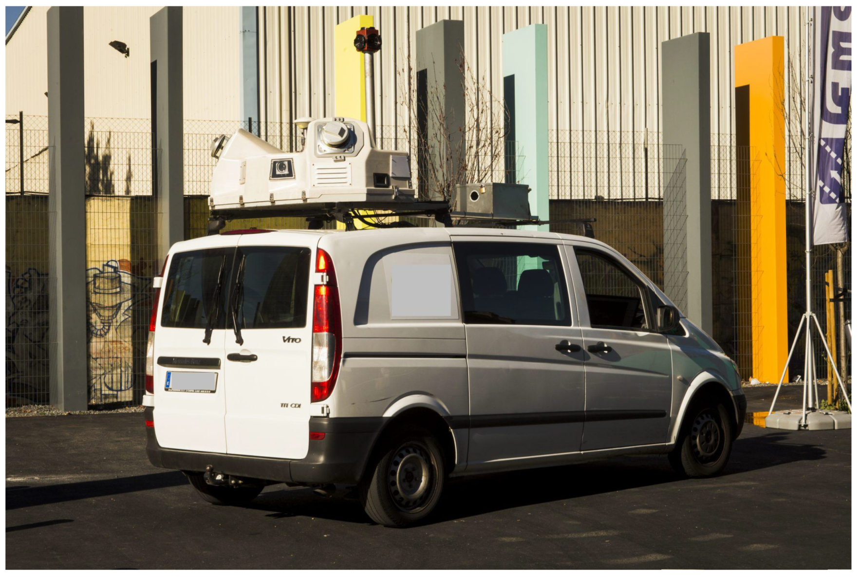The number of studies related to point-cloud processing and process automation for element identification in road infrastructures has increased significantly through the use of mobile LiDAR systems (MLSs), in which the LiDAR sensor is installed on a vehicle and acquires data while moving [11]. MLS allows data to be captured from close distances, providing points with small footprint size and high accuracy. The MLS has a navigation system with a GNSS (Global Navigation Satellite System) receiver and an Inertial Measurement Unit (IMU) that allows the position of the sensor, its direction and orientation to be known at every moment. Thanks to this, the MLS manages to capture a three-dimensional and georeferenced point cloud that accurately characterizes the geometric configuration of transport infrastructures with longitudinal routes over the territory (streets, roads, highways, highways, railways, etc.) [11,12,13].

Some studies have analyzed roads in rural areas, such as [14,15,16] or [17], which developed an effective method to generate a Digital Terrain Model (DTM) with high spatial resolution (0.25 × 0.25 m). Nevertheless, most research has been focused on the study of roads in urban areas, since the great disparity of elements present on the streets (curbs, vertical and horizontal signs, manholes, light poles, road pavement cracks, urban furniture, vehicles, etc.) makes the automation of any point-cloud segmentation process a difficult task. Having an accurate 3D model of the road surface, as well as an effective method to identify different road elements, is useful for maintenance studies and inventory of urban furniture and is essential for urban mobility analyses.

In the reviewed literature, some works focused on the determination of the road surface were found [18,19,20,21,22]. Among them, it is worth mentioning Gérezo and Antunes’ [23], in which a two-phased DTM was generated, first by identifying the terrain points and simplifying the point cloud and, later, by obtaining the DTM by means of the Delaunay triangulation on the terrain identified points. The authors of [24] proposed to align all the scan strips, identify the terrain points by applying the filtering method designed by [25] for Airborne Laser Scanner (ALS) data and generated a DTM. To improve its precision in areas without data, they proposed to merge their DTM with others of lower spatial resolution which were obtained using an ALS. Hervieu and Soheilian [26] proposed a method in which the edges of the road are identified to establish a geometric reference and subsequently reconstructing the surface. Guan et al. [27] developed an algorithm to segment the points of the road, grouping them into profiles according to the trajectory of the vehicle and generating a DTM with them afterwards.

On the other hand, certain articles have studied methods to efficiently segment different road elements that allow a more precise knowledge of the environment to be obtained. Some focus on the extraction of road markings [28,29,30,31,32,33], others on curbs [34,35,36], traffic signs [37,38,39,40], or on the determination of road cracks [41,42], among others.

In this context, research studies such as [43] stand out, in which an algorithm based on geometry and topology was proposed to classify elements of urban land (roads, pavement, treads, risers and curbs) that have subsequently been used as initial parameters in pedestrian accessibility studies [44].

The aforementioned research papers show that, among the scientific community, there is an interest in developing algorithms that automate the process of creating accurate 3D models based on point clouds acquired with MLSs in urban roads. However, we did not find, in the reviewed literature, studies that focus on the characterization of sidewalk metrics, which we consider fundamental in studies of pedestrian accessibility. Certain works focused on the detection of roadside trees, either by MLS point-cloud segmentation methods [45,46] or by using deep learning techniques [47,48]. Others, such as [43], proposed an algorithm based on geometry and topology to classify some urban elements (roads, pavement, treads, risers and curbs) that have subsequently been used as initial parameters of an accessibility study [44], but pedestrian accessibility needs a more precise characterization of sidewalks. It is necessary to detect other types of obstacles, such as benches, signs, streetlights, etc., as well as characterizing the pedestrian spaces knowing, with precision, width, slope, free spaces for pedestrians and roughness of the ground to identify, for example, tiles in bad condition, etc.; all this information was collected in the 3D model that we generated.

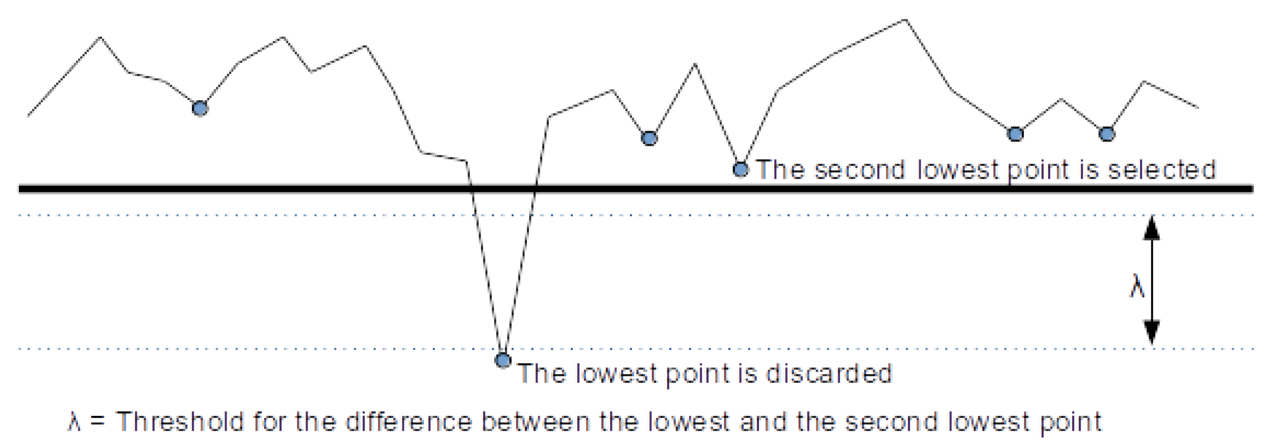
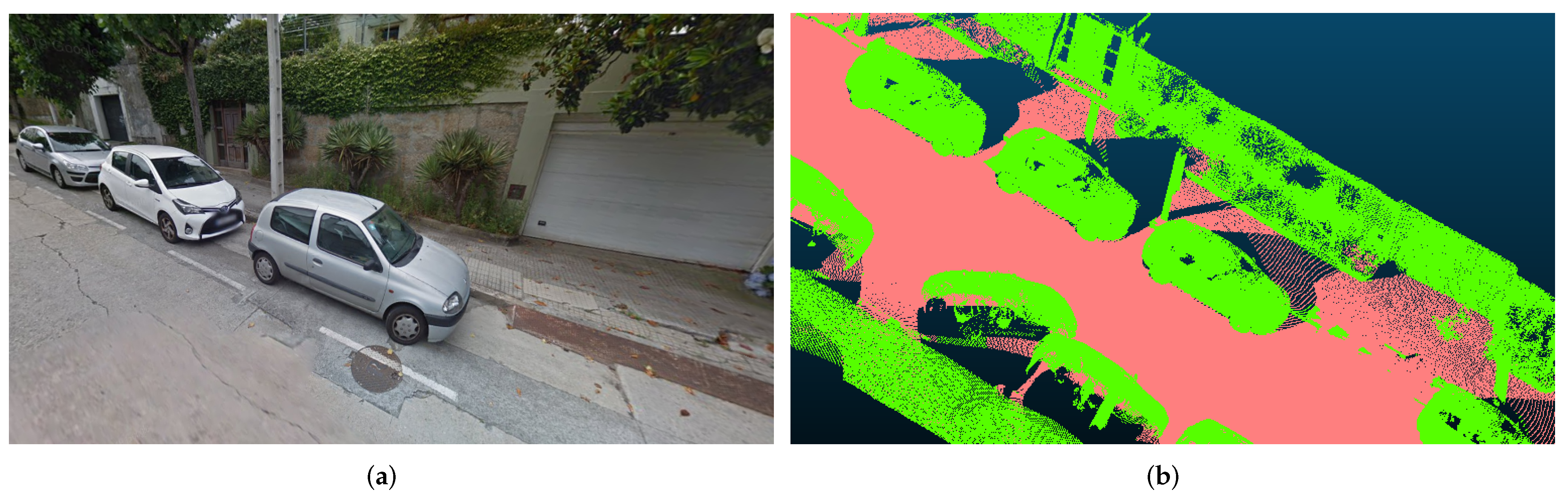
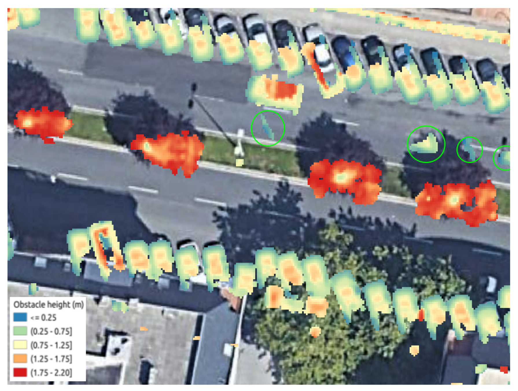
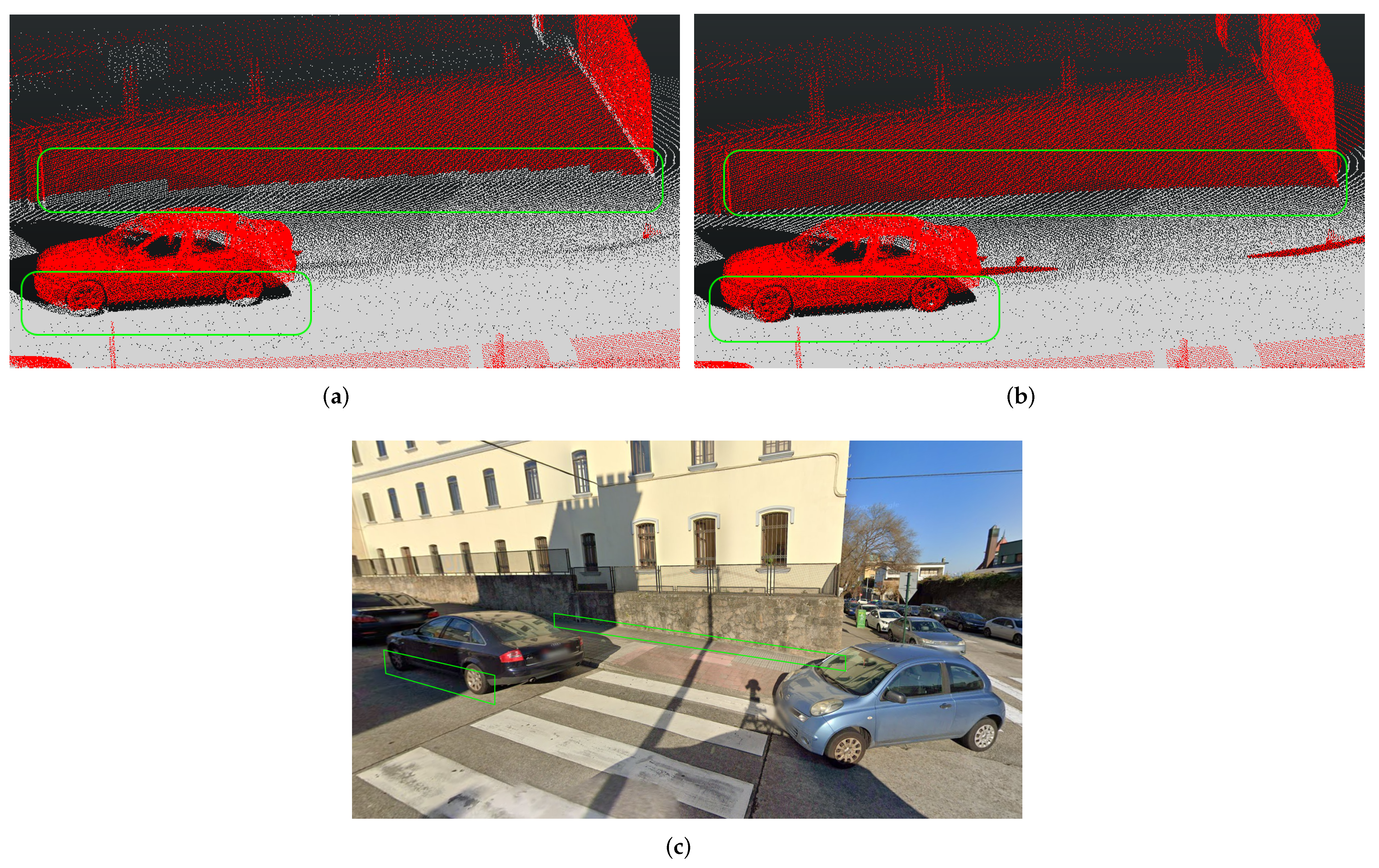
In addition, the automatic processing of MLS point clouds entails the solution of certain common problems that have not been accurately solved yet and of which we highlight two. The first one is the existence of obstacles in the road, mainly caused by vehicles or urban furniture that prevent the laser from acquiring data on the back, generating obstructions and creating areas without information in the point cloud. The second problem is due to the echoes produced by the laser pulse when it encounters glass surfaces (vehicles, windows and shop windows, among others) or vegetation, which cause double measurements of the points and must be eliminated, since they make it difficult to segment the cloud.

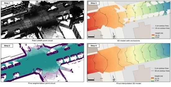
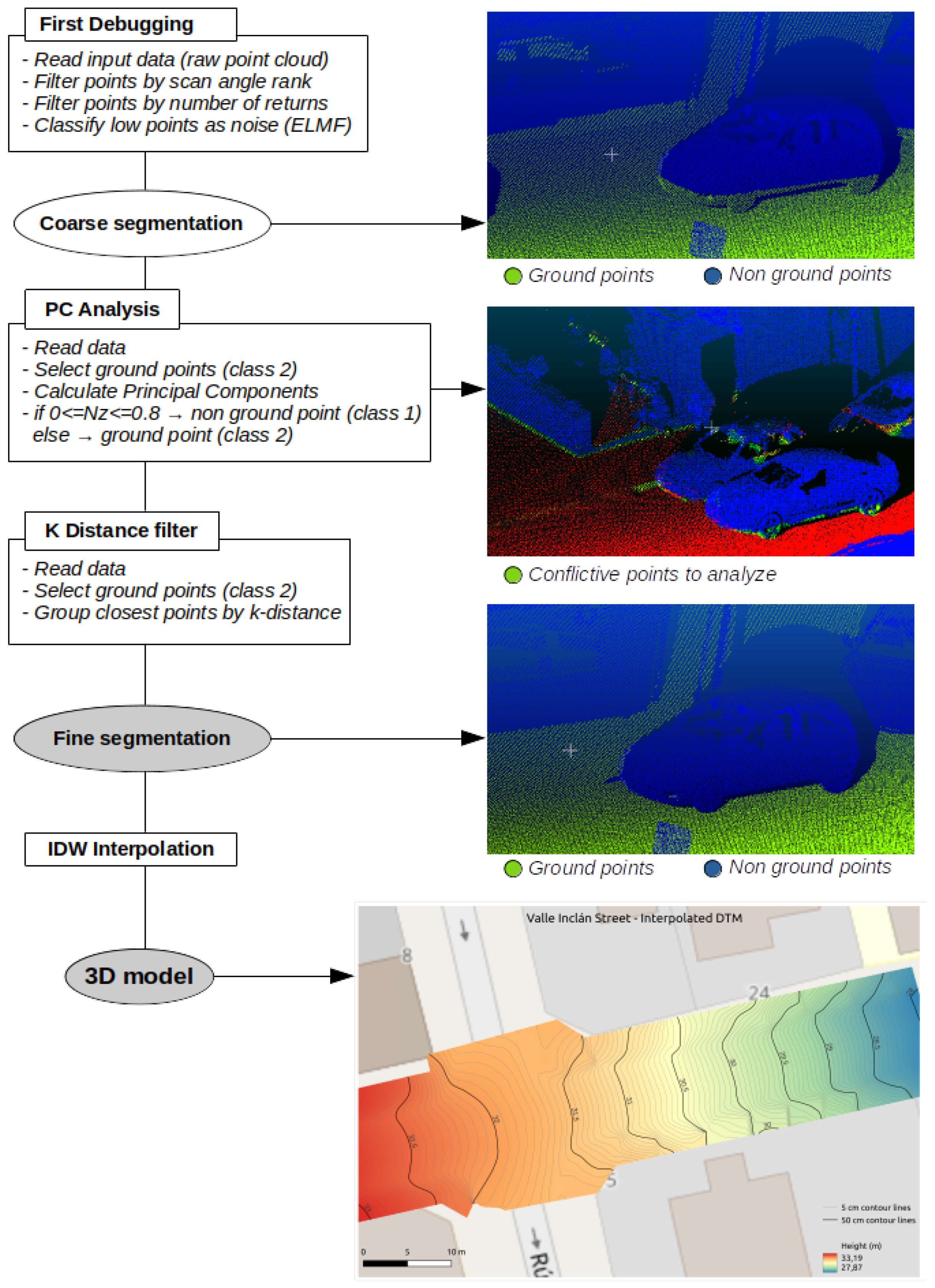
This paper proposes a method that made it possible to generate a 3D model of the urban road automatically, discriminating the points belonging to the terrain from the rest of the obstacles and simultaneously solving the above three problems. The algorithm works directly on the raw point cloud, using the Point Data Abstraction Library (PDAL). First, it removes the echoes, then it segments the cloud into terrain points and no terrain points; it determines the location of all obstacles, interpolates over the obstructed areas and, finally, generates a complete 3D model with great precision and spatial resolution. This model is essential in the latest pedestrian accessibility studies, as has already been demonstrated in the Big-Geomove project. In this project, we worked on the integration of multiple data sources for the parameterization of road characteristics in urban environments near schools. In particular, we worked with massive data sources for the characterization of roads, such as LiDAR point clouds obtained by mobile scanning devices. This information was complemented with geolocalized information provided by the students of the schools through participatory processes. With all the information, pedestrian safety indicators were elaborated to zone each road space according to its validity as a pedestrian travel zone. Conditional cumulative cost surface techniques were also applied to calculate optimal pedestrian routes in urban areas based on the conditioning factors of the zoning defined by the pedestrian safety indicators. However, for this, it was essential to model, from the three-dimensional LIDAR point cloud, a 3D surface of the space available for pedestrian transit. This methodology for obtaining urban road 3D models for pedestrian studies from LiDAR data is the process described in this article. The developed algorithms and LiDAR data used in this project are freely licensed and available for use in further research, as mentioned in this text.

In Section 2, the study area, the specifications of the MLS equipment used, the characteristics of the acquired point cloud and the details of the developed algorithm are exposed. Section 3 describes the obtained results, in areas with a high density of points as well as in regions with no data. In Section 4, the results are discussed and, in Section 5, the main conclusions of the paper are drawn.

2. Materials and Methods

2.1. Test Site and Input Data

The proposed method focuses on the analysis of urban roads, which is why four streets located in the cities of A Coruña and Ferrol (Galicia, Spain) were selected as a case study. The two streets of A Coruña, Virrey Osorio and Valle Inclán, were passable by vehicles and were composed of road, curb, pavement and building. In the captured scenes, there were multiple parked vehicles, which caused obstructions in the acquired point cloud. The two streets of Ferrol (Galiano and Real) were pedestrian areas, with multiple street furniture and pedestrians, which added some complexity to the segmentation of the point cloud.

Table 1. Studied streets metrics.

Street	No. Points	Length (m)	Width (m)	Z min (m)	Z max (m)
Galiano	97,472,943	296	12	13.48	25.25
Real	105,243,479	391	9	10.49	25.34
Virrey Osorio	48,240,018	467	15	13.03	37.45
Valle Inclán	38,712,115	458	15	14.38	41.27

describes some metrics of the scenes analyzed.

The equipment used for the acquisition of the point cloud was the Lynx Mobile Mapper M1 from Optech (Figure 1), composed of two LiDAR sensors that allowed us to perform the acquisition of up to 500,000 points per second, with a 360° field of view (FOV) (each scanner). The team also had 4 cameras of 5 Mpx, all of them bore sighted to the LiDAR sensors, and an Applanix POS LV 520 positioning and navigation system that used Trimble GNSS receivers.

Table 2. Optech Lynx M1 MLS technical specifications.

Item	Specifications
Number of LiDAR sensors	1–2
Camera support	Up to 4 cameras with scalable frame areas
Maximum range	200 m, 20%
Range precision	8 mm, 1 $\sigma$ under test conditions
Absolute accuracy	± 5 cm
Laser measurement rate	75–500 Hz programmable
Measurement per laser pulse	Up to 4 simultaneous
Scan frequency	80–200 Hz programmable
Scanner field of view	360${}^{°}$ without obscurations
Power requirements	12 VDC, 30 A max. draw
Operating temperature	from −10 ${}^{°}$C to 40 ${}^{°}$C (extended range available)
Storage temperature	from −40 ${}^{°}$C to +60 ${}^{°}$C
Relative humidity	0–95% non-condensing
Laser classification	IEC/CDRH class 1 eye-safe
Vehicle	Full adaptable to any vehicle

shows the main parameters of the equipment. Detailed technical specifications can be found in [49]. In [50,51], the characteristics of the equipment are analyzed.

Each piece of equipment, made up of two LiDAR sensors, a positioning system and RGB cameras, acquired the data independently and the information was linked by means of a GPS (Global Positioning System) time stamp. The result was a cloud with points every 3 cm (approximate density of 1000 points/m) and with geometric and radiometric information structured for each point according to P = (X, Y, Z, I, ts, rn, etc.), which indicate the 3D coordinates, intensity value, time stamp of acquisition of the point, return number, etc. Figure 2 shows an example of the raw point cloud on Valle Inclán street (A Coruña). The images from the cameras served, in this paper, as an element of verification of the gathered results.

The point clouds were acquired as initial data for the Big-Geomove project, with the purpose of knowing the dynamics of school mobility and its relationship with the technical conditions of the roads used in the area, using high-precision 3D models and spatial resolution. These models allowed us to study the roads in detail; both transversal and longitudinal visibility and slope analysis were carried out and obstacles for pedestrians and wheelchair users, among others, were identified. The gathered information was subsequently used to conduct a study on urban pedestrian mobility, where the configuration of the spaces available for traffic was categorized in detail and impedance values for non-motorized mobility were provided. This information on the presence of obstacles, slopes, surface roughness, uneven terrain, etc. would not be feasible with another type of starting data, such as 2D or DTM cartography with larger cell sizes.

The point clouds used in this project made up a total of 12 km of road and are currently available as ground truth for researchers under the Attribution 4.0 International https://creativecommons.org/licenses/by/4.0/ (CC BY 4.0) license in https://cartolab.udc.es/geomove/datos/en/ (CartoLAB/data).

2.2. Algorithm

The algorithm is divided into two phases (Figure 3). The first phase allows one to eliminate outliers and create a coarse segmentation between terrain points and non-terrain points. In the second phase, the segmentation is refined and the 3D model is obtained. The input data are raw point clouds and the resulting outputs are two different files. The first result is a point cloud divided into non-terrain points and terrain points, collected in a field called classification, with values of 1 and 2, respectively, according to https://www.asprs.org/a/society/committees/standards/LAS_1_4_r13.pdf (LAS specifications V. 1.4). The second result is a 3D model in raster format, with a possibility to customize the spatial resolution according to the requirements of the current project. The algorithm was developed using PDAL and Geospatial Data Abstraction Library (GDAL) open source libraries. This can be consulted and downloaded from https://gitlab.com/cartolab (Gitlab-Cartolab) or used directly in https://www.qgis.org/en/site/ (QGIS) through the https://plugins.qgis.org/plugins/pdaltools/ (PDAL Tools) and the https://plugins.qgis.org/plugins/tags/geomove/ (Geomove plugin) that we developed and implemented in all versions 3.X.

2.2.1. Debugging and Coarse Segmentation

The three-dimensional point cloud of the MLS scan maintains the https://www.asprs.org/a/society/committees/standards/LAS_1_4_r13.pdf (LAS specifications V. 1.4) file format. This is a binary file format that maintains information specific to the LiDAR nature of the data without being overly complex, so it has become the standard for working with LiDAR point clouds. The LAS format specifications were developed by the https://www.asprs.org/ (American Society for Photogrammetry and Remote Sensing (ASPRS)) from its version 1.0 in 2003 to its most recent version 1.4, Format Specification R15 9 July 2019. One of the values collected by this format is the scan angle range which collects the angle at which the laser spot is emitted by the system. Since the first uses of LiDAR were installed on aircraft, this angle is considered to be between +90 and −90 degrees, based on 0 degrees being NADIR. Although the LiDAR sensors installed in MLSs are capable of obtaining information at 360 degrees on the vertical plane of the sensor, the scan angle range values are still kept between +90 and −90 in the LAS format. Since the MLS sensor is normally installed on top of a light vehicle and our interest is to study the pavement characteristics where pedestrians can walk, a first filter is applied keeping the points below the horizontal line of the MLS sensor, with values of the scan angle range between +45 and −45 (Figure 4).

The algorithm started by eliminating all points outside the road and analyzing only those that were in a Scan Angle Rank of [−45, 45] from the Nadir, which allowed the cloud to be simplified by eliminating high areas that were not important for the analysis of the areas around the road. The points that did not belong to the first echo or return were also removed from the study. The objective was to work only with the pulses that hit solid surfaces since those that passed through other surfaces, such as vehicle windows or vegetation, caused certain problems when creating the segmentation. In this context, in [52], a method capable of detecting 3D objects using multiple LiDAR returns is exposed. Then, an Extended Local Minimum Filter (ELM) was applied to the rest of the point cloud. This filter is an implementation of the method described in [53] and allowed us to filter out low points as noise. The ELM rasterizes the points into a defined cell size. For each cell, the lowest point is considered noise if the next lowest point is at a given threshold above the current point (Figure 5). If it is identified as noise, the difference between the next two points is also considered, identifying them as noise if necessary and continuing the process until a neighboring point within the set threshold is found. At that point the iteration over the analyzed cell stops and the process continues on the next cell.

In this implementation of the method, 1 m cells were used, identifying the lowest point in each of them and comparing the height differences between all the points of the cell iteratively. If the difference between the analyzed point and its closest adjacent point was more than 0.25 m, then it was classified as a low point, if not, it maintained its classification and the process continued until the analysis of all the points in the cell had finished.

Finally, based on [54,55], outliers were identified using a method based on two steps; the first allowed us to calculate a threshold value and the second to identify outliers. To calculate the threshold, an average distance from each point to its 30 adjacent points was estimated. From all these mean distances, a global mean ($\overline{\mu }$) and a standard deviation ($\sigma$) were calculated. Finally, the threshold was calculated using m = 3 as the multiplying factor of the standard deviation. Once obtained, the distances between points were analyzed repeatedly. If the distance between them was greater than the established threshold, the analyzed point was an outlier and it was classified as a non-terrain point.

2.2.2. Fine Segmentation and 3D Model Creation

Two improvements were applied to the segmented cloud, which allowed us to refine the segmentation in the most difficult regions, such as the transition areas between the terrain and vertical elements (buildings, vehicles, etc.). A Principal Component Analysis (PCA) was applied, decomposing each point into its Normal-X, Normal-Y and Normal-Z eigenvectors in relation to its 30 closest adjacent points. For each point, the value of its Normal Z was studied. If it was in the range [0, 0.8], it was classified as a non-terrain point (class 1), since it indicated vertical planes such as building facades, vehicles, obstacles, etc.; if it was in the interval [0.8, 1], it was kept as a terrain point (class 2). A K-distance analysis was performed to identify groups of misclassified points, calculating the distance from each point to its 300 adjacent points. If this distance was less than 0.7 m, both points were classified within the same category, but, if it was greater, they were classified in different categories and the analyzed point was moved to the non-terrain point class. The terrain points of the resulting cloud were selected and, with them, a 3D model was generated whose pixel values were the means of the heights of all the points of the terrain point class contained in that pixel. The chosen pixel size was 5 cm since it was considered an adequate spatial resolution to be able to accurately typify all the distinctive features of pedestrian pathways. In our case, it was possible to typify slopes, both transverse and longitudinal, break lines caused by curbs or traffic islands and obstacles for pedestrians, such as street lamps, benches, or trees, among others.

Finally, during the data acquisition phase, the presence of multiple vehicles and urban furniture elements prevented the acquisition of points in certain regions, which caused obstructions that made it impossible to generate a complete and continuous 3D model, as it can be seen in Figure 6. For this reason, at the end of the algorithm, the module https://grass.osgeo.org/grass80/manuals/r.fill.stats.html (r.fill.stats), from the https://grass.osgeo.org/ (GRASS-GIS) library, was executed, which allowed a height value to be assigned to each pixel without data, based on the height of its adjacent cells. In this case, the interpolation mode used was the spatially weighted mean, equivalent to an Inverse Distance Weighted (IDW) interpolation. To assign the height to each pixel, the 8 closest cells were analyzed.

2.3. Three-Dimensional Model Quality Test

2.3.1. Three-Dimensional Model from Real Data

To verify the altimetric accuracy of the 3D model created and to validate the strength of the method in the areas with real data, the heights obtained were compared with those of 1000 points of known height, randomly selected from the point cloud using the Bash https://linux.die.net/man/1/shuf (shuf) tool. First, the mean values and interquartile ranges for the differences in heights were calculated and, later, a global value of RMSE (Root-Mean-Square Error) was estimated for each scene.

In addition, to verify the improvement of the fine segmentation with respect to the coarse segmentation, we quantified the number of points categorized as ground, both in the coarse segmentation and in the fine segmentation. This study was carried out on the entire point cloud in the four analyzed scenes. For each scene, we counted (I) the number of points of the raw scene; (II) the number of points analyzed, once the outliers had been filtered and the Scan Angle Rank restriction [−45, 45] from the Nadir had been applied to eliminate the points belonging to the high areas of the buildings, which were not of interest in the road analysis; (III) the number of points classified as ground in the coarse segmentation; (IV) the number of points classified as ground in the fine segmentation; (V) the percentages of ground–non-ground in respect to the entire raw point cloud and in respect to the analyzed point cloud.

This analysis aims to validate (I) the ability of the algorithm to filter and analyze only the points in the road environment, discriminating them from the rest of the point cloud and making the model more efficient, and (II) the ability of fine segmentation to work correctly on point clouds in the transition zones between orthogonal planes, which are usually the most problematic regions in LiDAR point-cloud segmentations.

2.3.2. Three-Dimensional Model of Occluded Areas

To validate the interpolation method used in shadow areas, new scenes were generated, including five occlusions in each of them, with sizes between 50 and 2850 pixels, simulating patterns similar to the real shadow areas, both on the road and on the pavement, with an arbitrary distribution, as shown in Figure 7.

Subsequently, these new scenes were processed with intentional occlusions. The heights obtained in the areas without data were compared with those obtained in the scenes with real data. This comparison was made by calculating the difference between the two rasters (3D model from real data and interpolated 3D model from intentional occlusions) and by analyzing the values of pixel count (total number of pixels that made up the occlusion), mean error (mean value of difference in height), min error and max error (minimum and maximum height difference values) in each of the occlusion polygons.

2.4. Obstacle Detection

Being aware of the importance of 3D models in mobility studies and taking into account that one of the main tasks of the Big-Geomove project was to analyze pedestrian mobility in urban areas, in addition to obtaining an accurate 3D model of the road, elements that hindered mobility, for both pedestrian and wheelchair users, were also detected. These obstacles were incorporated as impedance surfaces in the subsequent accessibility analysis.

For this matter, all the elements found (curbs, benches, lampposts, trees, etc.) were classified according to their influence on the type of mobility, considering, as obstacles for pedestrians, all those elements with a relative height from the ground or a difference in height in respect to their neighbors, called Height Above Ground (HAG), greater than 25 cm and as obstacles for wheelchair users all those that had an HAG of over 5 cm. Figure 8 shows an example of the pedestrian obstacles detected. Furthermore, certain pixels identified as obstacles on the road (green circles), probably due to the presence of moving vehicles at the time of data acquisition, which caused small areas without data on the road, can also be seen. These areas were treated in the same way as parked vehicles, i.e., by applying an IDW interpolation on the closest ground points.

The obstacle detection analysis was developed by iteratively calculating, on all the points previously identified as ground (class 2), the difference in height between each analyzed point and its neighbors of the 3D point cloud obtained after the fine segmentation. The HAG value of each point was stored in a new numerical field as a normalized height above which the two types of obstacles could be differentiated based on the type of mobility (pedestrian or wheelchair). Non-ground elements, thus, obstacles generated a space on the ground plan that was rasterized to create no-pass zones in the possibilities of walking on the 3D model created. The developed algorithm detected and generated the complete street ground surface and the surfaces occupied by pedestrian and wheelchair obstacles. This algorithm was published on https://gitlab.com/cartolab/geomove/geomove_pipelines (Gitlab/CartoLAB).

The obstacle raster zones were used together with the created 3D model to generate different impedance surfaces according to the degree of pedestrian mobility. These impedance surfaces are used in cost–distance algorithms on Geographic Information Systems (GISs) [56] to identify optimal pedestrian routes in urban environments (Figure 9).

3. Results

3.1. Debugging and Coarse Segmentation

The algorithm eliminated practically all the outliers and low points in the coarse segmentation and correctly segmented most of the points in the cloud. However, in transition zones between the ground and certain vertical planes, errors such as those shown in Figure 10a were found. Some vehicles or the lower parts of buildings were found to have been erroneously typified as terrain points, requiring further debugging.

3.2. Fine Segmentation and 3D Model Creation

A PCA analysis identified the transition areas between orthogonal planes and correctly segmented the point cloud in them. A K-distance analysis improved the segmentation of groups of points that had been previously assigned to the same category due to their similar geometric characteristics, but that actually belonged to different objects. Figure 10b shows how these problem regions were correctly segmented. Ramps were also correctly identified as ground points and curbs as vertical elements the height difference of which (between the ground of the sidewalk and that of the road) was taken into account to create the 3D model of the urban area for pedestrians.

As can be seen in the green boxes that are highlighted in Figure 10a, corresponding to the coarse segmentation, the points located in transition zones between orthogonal planes, such as the transitions between ground and vehicles or buildings, had segmentation problems. In Figure 10b, it can be verified that the fine segmentation allowed the algorithm to segment the points of the cloud in these transition zones and even define the location of the curbs and differentiate them from the building access ramps (according to their Nz component), which had not been considered in the coarse segmentation.

Finally, Figure 11 shows an example of the 3D models resulting from the segmented clouds for each of the analyzed scenes. In it, the initial point clouds, the models created with the occlusions due to lack of data and the interpolated models, completely generated in spite of the occluded areas, can be observed. In these final models, the boundary lines between the roadways and pavement, as well as the transitions of the slopes between perpendicular streets, are also clearly discernible.

3.3. Segmentation Quality Test

In order to evaluate the point-cloud segmentation method, a subset of Valle Inclán street was analyzed. The selected subset was a point cloud of 2,506,108 points located in the center of the scene that had a representative layout of the analyzed streets which included ground, trees, facades, vertical signs, vegetation, cars and people (Figure 12). The resulted fine segmentation was compared with a manually segmentation (Figure 13). The following performance metrics are defined:

$$Precision=\frac{TP}{TP+FP}$$

(1)

$$Recall=\frac{TP}{TP+FN}$$

(2)

$$F_{score}=2\ast \frac{Precision\ast Recall}{Precision+Recall}$$

(3)

where TP, FP and FN are the number of true positives, false positives and false negatives (

Table 3. Segmentation criterion results.

True Positives	False Positives	False Negatives	Analyzed Points
2,498,449	3289	4370	2,506,108

). The results of precision, recall and F-score performance metrics are shown in

Table 4. Precision, recall and F-score for analysis of the segmentation quality.

Precision (%)	Recall (%)	F-Score (%)
99.87	99.82	99.85

.

The results of the precision, recall and F-score analysis show very high values, which demonstrates the efficiency of the method in MLS point clouds with similar characteristics to those of this work.

As can be seen in Figure 13, most of the false positives were located in the transition zones between orthogonal planes, either near the buildings, such as the group of points in the upper left part of the image, or in the lower part of the vehicles. False negatives appeared mainly on sidewalks in the proximity of occlusion areas. On the other hand, almost no false negatives were located on the road.

3.4. Three-Dimensional Model Quality Test

3.4.1. Three-Dimensional Model from Real Data

As it can be seen in Figure 14, the height difference values between the 3D model and the 1000 random points are mostly between −20 and 20 mm. Only two outliers were found in Galiano Street (Ferrol), where the height of the model was lower than that of the random points 190 and 100 mm. The RMSE values were also lower than 10 mm in three of the four scenes analyzed and only rising to 12 mm in Galiano Street (Ferrol).

3.4.2. Three-Dimensional Model of Occluded Areas

As it can be observed in

Table 5. Occluded areas’ validation results.

Street	Occlusion	Pixel Count	Mean Error (mm)	Min Error (mm)	Max Error (mm)
Valle Inclán	1	2404	3	−51	58
Valle Inclán	2	1694	19	−36	83
Valle Inclán	3	685	2	−16	14
Valle Inclán	4	1435	4	−21	19
Valle Inclán	5	537	26	−21	75
Virrey Osorio	1	1931	3	−30	40
Virrey Osorio	2	1604	3	−31	46
Virrey Osorio	3	2850	1	−65	56
Virrey Osorio	4	1332	19	−25	34
Virrey Osorio	5	1010	33	−68	146
Real	1	78	−1	−2	1
Real	2	77	0	−2	2
Real	3	82	0	−2	2
Real	4	524	−3	−10	6
Real	5	50	0	−1	1
Galiano	1	306	3	−2	7
Galiano	2	155	−1	−3	2
Galiano	3	172	4	0	6
Galiano	4	168	1	−3	5
Galiano	5	129	2	−1	3

, in the polygons of both pedestrian streets Real and Galiano (Ferrol), the mean errors of each polygon remained below 4 mm and the maximum errors below 10 mm in all cases. In the two streets with vehicular circulation, the mean differences were also lower than 4 mm in six of the ten analyzed polygons; however, in the four remaining polygons, these values rose to 19 mm (in two polygons), 26 mm and 33 mm. Of these four errors in the interpolation, two of them were made in polygons located in transition areas between the pavement and the road (polygon 2 of Valle Inclán street in A Coruña, with 19 mm and polygon 5 of Virrey Osorio street, also in A Coruña, with 33 mm) and another on an access ramp to a private car park (polygon 5 of Valle Inclán street, with a 26 mm error). In the case of maximum errors, the range was established between −68 mm and 146 mm, also corresponding to polygon 5 of Valle Inclán street. The rest of the polygons kept their maximum errors in the interval [−65 mm, 83 mm].

In the fine segmentation verification analysis, as can be seen in

Table 6. Fine segmentation validation.

Street	Galiano	Real	Virrey Osorio	Valle Inclán
No. points of raw scene	97,472,943	105,243,479	48,240,018	38,712,115
No. debugged points	54,497,047	58,223,758	28,873,479	35,561,091
No. ground points in coarse segmentation	39,167,982	41,042,579	21,470,400	24,947,120
No. ground points in fine segmentation	29,889,691	35,401,819	20,395,362	23,652,141
Difference (coarse–fine)	9,278,291	5,640,760	1,075,038	1,294,979
% Variation	23.69	13.74	5.01	5.19
% Ground points from analyzed points	54.85	60.80	70.64	66.51
% Ground points from raw point cloud	30.66	33.64	42.28	61.10

, the difference between the percentage values of ground from the total points of the raw data and the percentage of ground from the analyzed points were substantial, reaching almost double in some scenes. This fact verified the ability of the algorithm to simplify and purge the uninteresting points of the raw point cloud and work only with the necessary points, optimizing data processing. In the case of the two pedestrian streets (Galiano and Real), the scenes had only 30.66% and 33.64% ground in respect to the total points, respectively, and, once the initial filters were applied, the percentages rose to 54.84 and 60.80%.

The number of ground points was lower in the fine segmentation than in the coarse segmentation in all the analyzed scenes. This fact shows that the PCA and K-distance analyses correctly segmented the point clouds in the conflicting regions, of transition between orthogonal planes.

The fine segmentation offered significant purification percentages, eliminating more than 5% of points that did not belong to the soil. This allowed us to better define the model representing the pedestrian walking surface.

Finally, the fact that the percentage of ground was greater in the streets that could be traversed by vehicles than in the pedestrian streets indicates the presence of a greater number of conflictive zones in the pedestrian streets, due to the constant presence of street furniture, such as benches, planters, etc., in addition to the greater presence of nearby buildings, directly located on the main road. In these cases, fine segmentation offered more relevant improvement percentages, with improvements of more than 20% of the points defining the ground.

3.5. Processing Time

Table 7. Scene processing time.

Task	Galiano St.	Real St.	Virrey Osorio St.	Valle Inclán St.
Initial debug	00:17:41	00:19:21	00:11:52	00:09:31
Nz processing	00:32:44	00:35:44	00:18:59	00:15:40
K-distance	01:52:46	02:09:16	01:21:04	01:11:29
HAG processing	00:03:53	00:04:24	00:02:24	00:02:00
3D model export	00:00:20	00:00:26	00:00:16	00:00:15
Total time	02:47:24	03:09:11	01:54:35	01:38:55

shows the processing times that were used to obtain the 3D model from the raw point cloud, itemized by task. In this study, our team had an Intel® Core™ i7-4702MQ CPU @ 2.20 GHz 4 core processor with 12 GB of RAM and the operating system was Linux Ubuntu 18.04 64-Bit.

4. Discussion

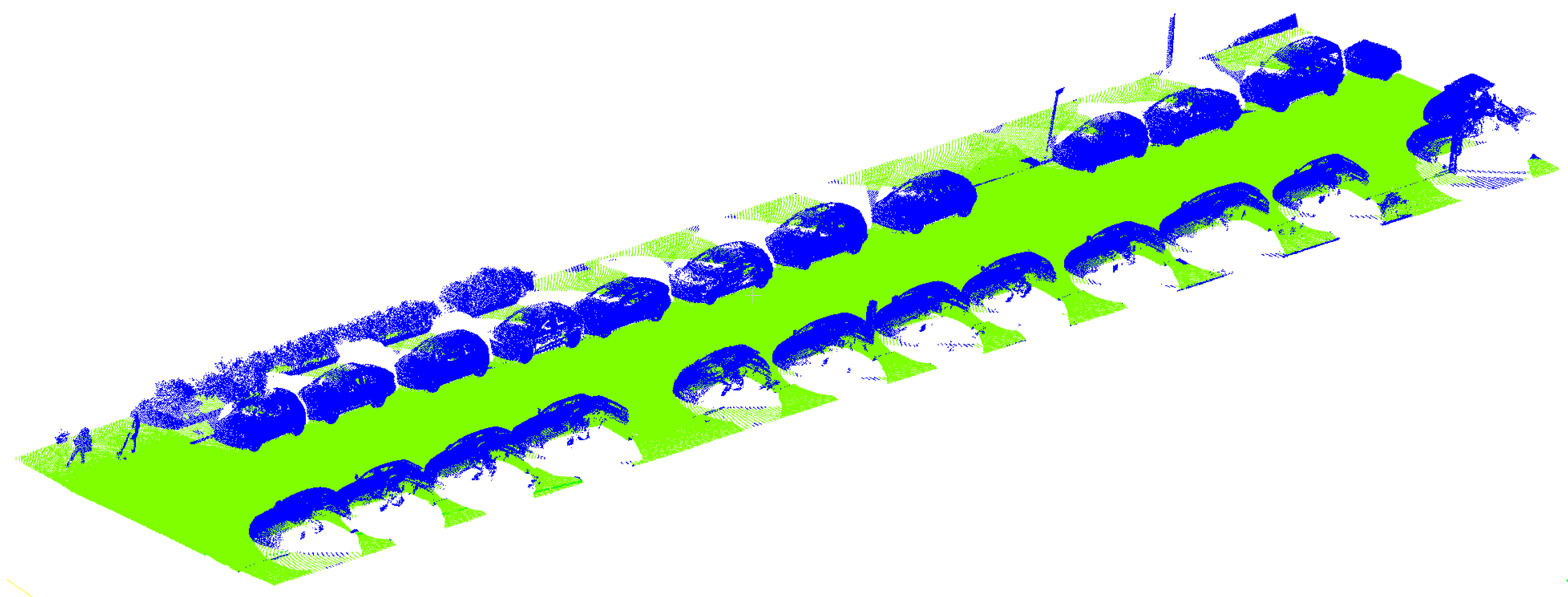
The work carried out in this research study made it possible to create an efficient method to discriminate the points belonging to urban roads from the remaining elements in the analyzed scenes, from a raw LiDAR point cloud with the following information per point: P = (X, Y, Z, I, ts, rn, etc.). Two final products were generated, a segmented point cloud in *.las format and two 3D model in raster format, one with the road surface without interpolation and the other with interpolated shadow areas, generating a continuous model (digital surface model).

The proposed method differs from others such as [27], since our algorithm was able to analyze all the points of the acquired cloud and even group multiple scenes, regardless of the number of trajectories used by the vehicle to gather data, which significantly sped up the process.

The results of the fine segmentation show very high precision, recall and F-score values. These metrics were compared with those of other similar studies such as [57,58,59] and the results obtained are similar and even better, which demonstrates the ability of the algorithm to correctly segment the MLS point clouds with similar characteristics used in this study.

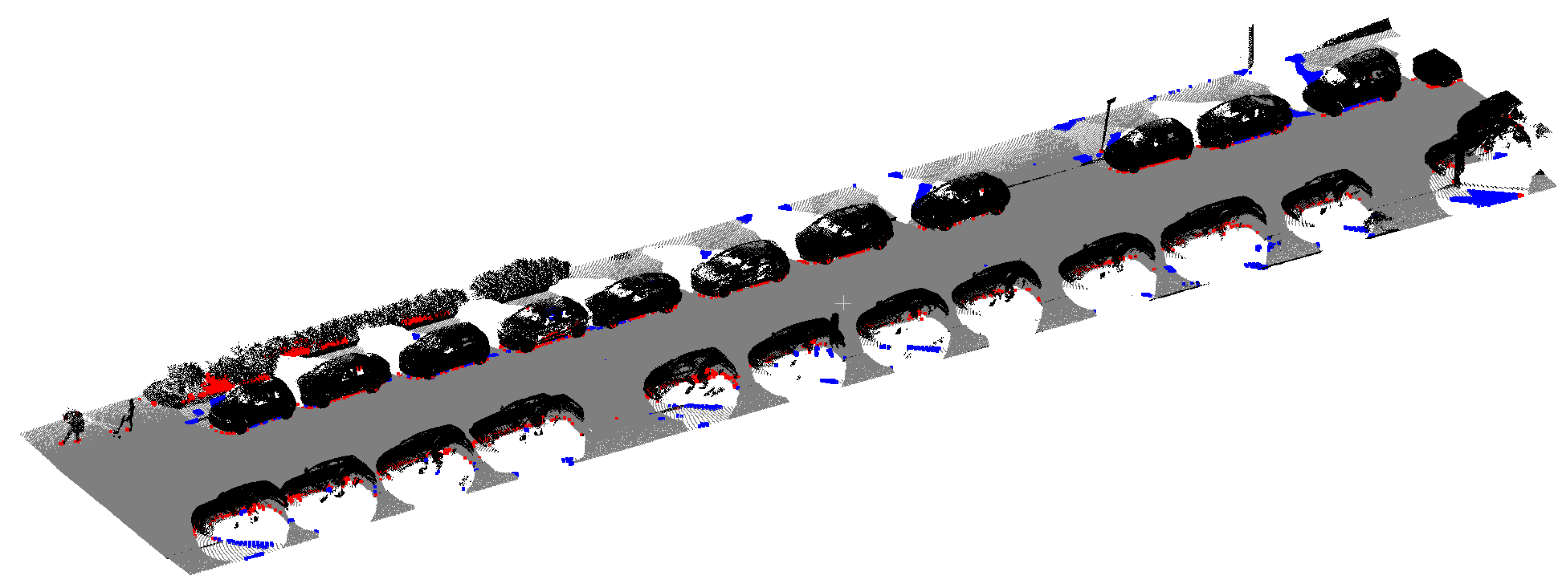
As expected, most of the false positives were located in the transition zones between orthogonal planes, near the buildings, such as in the case of cars, and false negatives were located on sidewalks, which are usually the most difficult areas to segment due to the existence of shadow areas in MLS data.

As this segmentation was intended to be used to generate impedance surfaces for an accessibility analysis and the 3D models used in these task must have high spatial resolution and precision in the segmentation, we decided to prepare the algorithm to avoid false positives even though we had to increase the number of false negatives, because these are easily solvable with the interpolation method used later.

Likewise, the vertical parts of the curbs were intentionally segmented as non-floor because, in the accessibility analysis, they are obstacles that both pedestrians with mobility problems and wheelchair users must overcome.

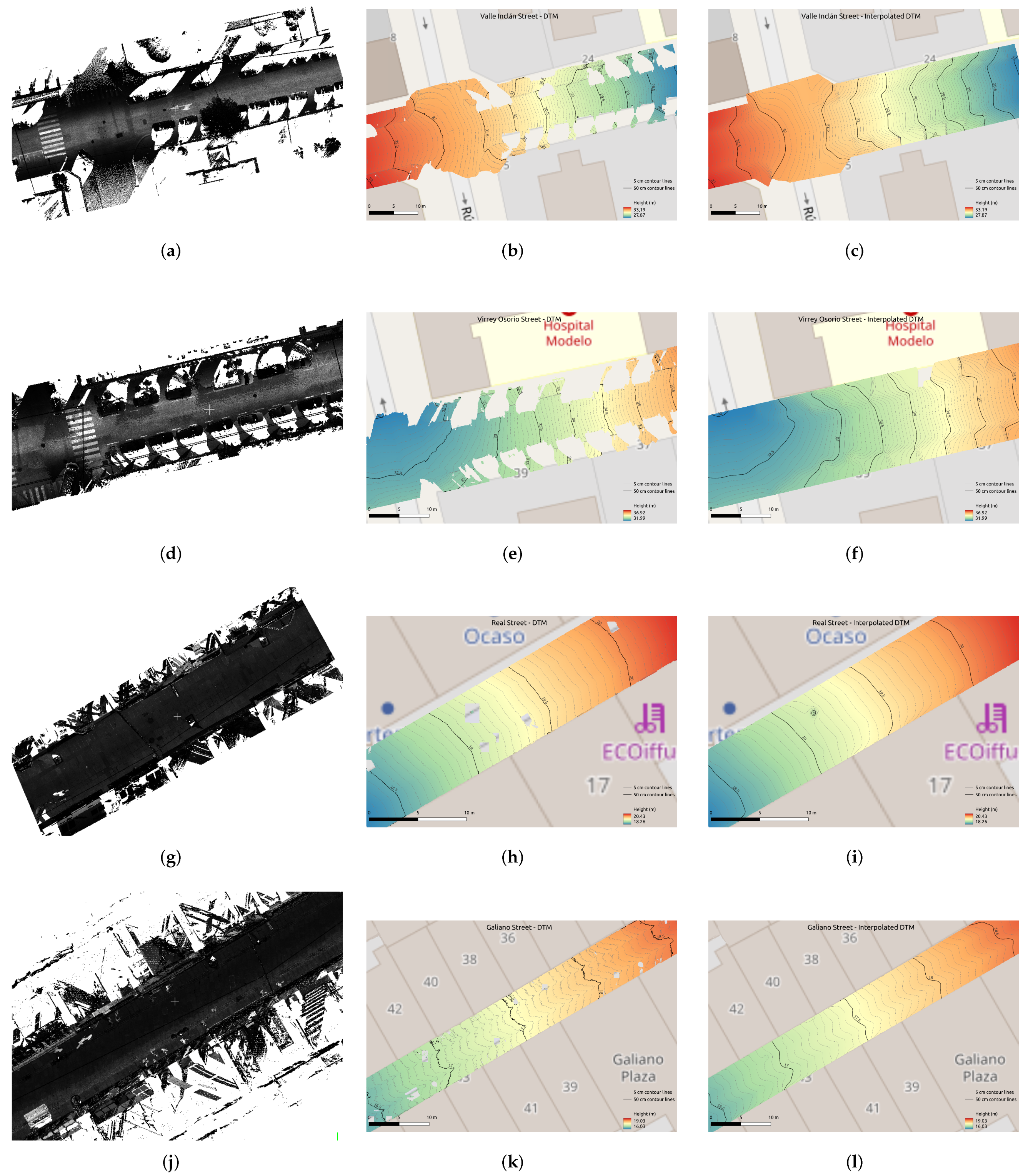
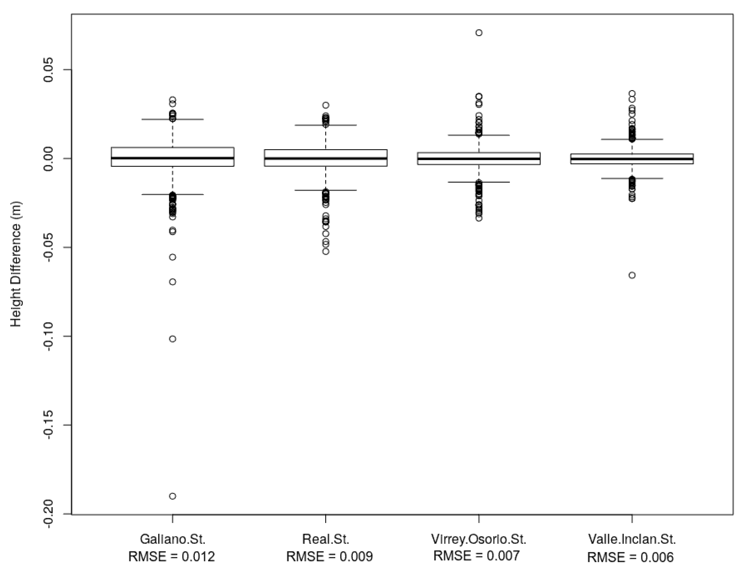
The validation of the 3D model algorithm was developed in two phases, one for the areas with real data and the other for regions without data, in which the algorithm interpolated with the values of the adjacent points to generate a continuous model. The results show that the method was more efficient when the density of points in the scene was high, obtaining mean errors close to 0 and maximum errors of 20 mm, as it can be seen in Section 3.4. On the contrary, it had limitations in regions without data, in which it was necessary to interpolate to generate a continuous model. In these areas, the mean errors were between 1 and 33 mm and the maximum errors between −68 and 146 mm. These errors corresponded to transition regions between pavements and roadways, showing that the interpolation method was not able to accurately locate the break lines and it joined adjacent points diagonally, making it a problem to identify curbs. This explains the obtained errors being lower in the two pedestrian streets (Real and Galiano) than in those passable by vehicles, since the occluded areas were smaller and required less interpolation. In the same way, the results are also better in flat areas, such as the center of the streets, than in transition areas between the pavement and the road.

Although the objective of this paper is not to reconstruct the lines of the curbs, the eigenvectors of each point were obtained with precision and the planes in which they were found were also defined. This knowledge opens a line of research in which we are currently working with the intention of reconstructing curb lines, even in areas without data, with which procedures for the automatic generation of differentiated 3D models could be applied for pavements and driveways. In the same way, as in the method by [24], the fusion of our model with others obtained from ALSs, even with lower spatial resolution, could be an affordable solution to improve precision in these conflictive areas.

It was also proved that the algorithm generated the models in processing times, as it can be seen in Table 7. No differentiating data was found in terms of processing times for scenes with a greater number of shadow areas, different slopes or the presence of road elements. Processing times depend solely on the performance of the computer equipment used and the amount of RAM available at the time of the analysis—in our case, a computer with 12 GB of RAM, which took approximately 3 h to process 100,000,000 points.

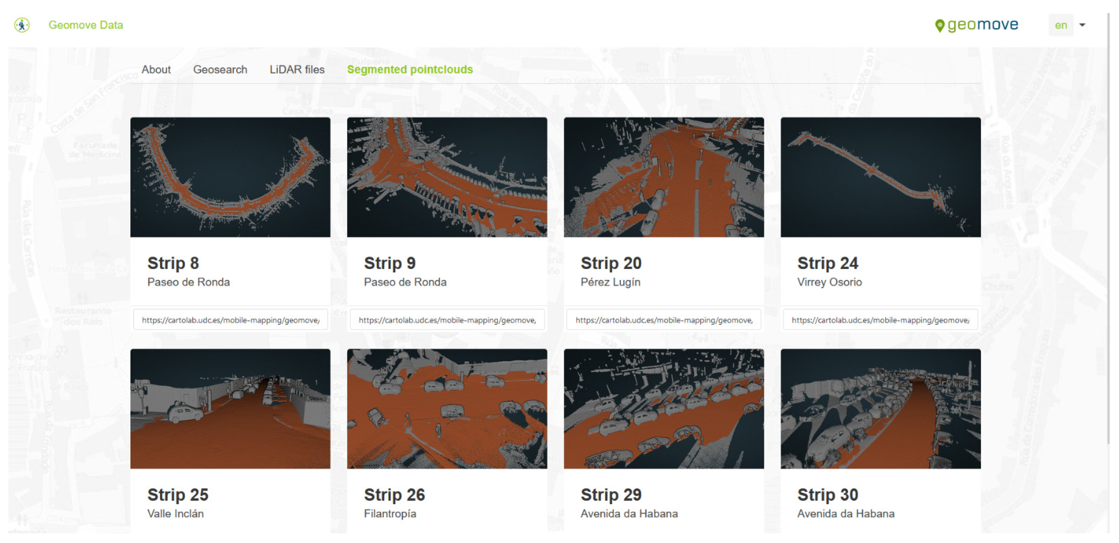
During the bibliographic review process, no similar free-licensed methods that allow one to obtain 3D models automatically were found. All the algorithms found had a proprietary license, so it was decided to implement the algorithm as a Plug-in in all versions of QGIS 3.X. In the same way, both the algorithm and the MLS data were published under the Attribution 4.0 International https://creativecommons.org/licenses/by/4.0/ (CC BY 4.0) license in https://gitlab.com/cartolab (Gitlab-Cartolab) and https://cartolab.udc.es/geomove/datos/en (Geomove/data), respectively, which offers an interesting data bank to be used in other investigations as ground truth. A screenshot of the Geomove LiDAR data download website can be seen in Figure 15.

5. Conclusions

Mobile LiDAR technology has proven to be an accurate and fast tool to obtain dense point clouds from urban roads without interrupting the usual pace of the city. For this paper, 12 km of urban roads were scanned and the proposed algorithm efficiently discriminated the point cloud acquired by the MLS, differentiating the points of the road from the rest of the urban elements and allowing us to automatically generate a 3D model of the road surfaces in due processing times. All existing elements over 25 cm in height on the road were considered as non-ground areas, thus impossible to be crossed by pedestrians. The rest of the road space was rasterized as a digital surface model with a cell resolution of 5 cm, taking advantage of the high density of points provided by the LiDAR sensor. This made it possible to accurately differentiate any small defect in the pavement that would make it more or less comfortable for a pedestrian to walk on. The average difference in the values of the dimensions of the 3D model created with respect to the values of the LiDAR point cloud did not exceed 20 mm, which achieves a high accuracy in the modeling of walkable surfaces. We could detect holes or defects in the pavements, as we can see in the sinkhole of 10–15 cm identified in Figure 11i.

The main problem with MLS point clouds in urban environments is the presence of occlusions (lack of data). The presence of vehicles parked on the side of the road and similar obstacles, such as containers or bus shelters, among others, prevent the laser beam from hitting the road. To fill in these areas without data, an interpolation method was used on the closest points to generate a complete and continuous model of the entire road surface. The accuracy achieved in this interpolation showed an average errors of less than 1 cm in most of the occluded areas, without exceeding 33 mm as the highest average difference. Only in situations where there were curbs a maximum difference of less than 15 cm was reached in some cases. In any case, this model proved to be efficient for urban mobility studies and, more specifically, in the Big-Geomove project, which used this modeled base surface to identify safe pedestrian routes in the urban areas analyzed. For this purpose, in addition to this model, different obstacles that impeded or hindered circulation, both for pedestrians and wheelchair users, such as curbs, lamppost, benches, stairs, etc., were detected. With these obstacles, different impedance surfaces were generated, which made it possible to identify the optimal pedestrian routes in urban areas, through the application of accumulated cost surface techniques.

As a continuation of this work, a line of research was opened with the main objective of developing a method to reconstruct curb lines. Having this line accurately available would allow differentiated 3D models for sidewalks and roadways to be generated, avoiding interpolation errors of occluded zones in the transition spaces between them.

References

1. Van den Berg, A.E.; Beute, F. Walk it off! The effectiveness of walk and talk coaching in nature for individuals with burnout-and stress-related complaints. J. Environ. Psychol. 2021, 76, 101641. [Google Scholar] [CrossRef]
2. Bratman, G.N.; Anderson, C.B.; Berman, M.G.; Cochran, B.; De Vries, S.; Flanders, J.; Daily, G.C. Nature and mental health: An ecosystem service perspective. Sci. Adv. 2019, 5, eaax0903. [Google Scholar] [CrossRef] [PubMed] [Green Version]
3. Ettema, D.; Smajic, I. Walking, places and wellbeing. Geogr. J. 2015, 181, 102–109. [Google Scholar] [CrossRef]
4. Soroush, A.; Der Ananian, C.; Ainsworth, B.E.; Belyea, M.; Poortvliet, E.; Swan, P.D.; Walker, J.; Yngve, A. Effects of a 6-months walking study on blood pressure and cardiorespiratory fitness in US and swedish adults: ASUKI step study. Asian J. Sports Med. 2013, 4, 114. [Google Scholar] [CrossRef] [Green Version]
5. Jelaian, A.V. Laser Radar Systems.; Artech House: Boston, MA, USA, 1992. [Google Scholar]
6. Borgogno Mondino, E.; Fissore, V.; Falkowski, M.J.; Palik, B. How far can we trust forestry estimates from low-density LiDAR acquisitions? The Cutfoot Sioux experimental forest (MN, USA) case study. Int. J. Remote Sens. 2020, 41, 4551–4569. [Google Scholar] [CrossRef]
7. Garcia, I.A.; Starek, M.J. Mobile and Airborne Lidar Scanning to Assess the Impacts of Hurricane Harvey to the Beach and Foredunes on North Padre Island, Texas, USA. In Proceedings of the AGU Fall Meeting Abstracts, San Francisco, CA, USA, 9–13 December 2019; p. IN51G-0716. [Google Scholar]
8. Gruen, A.; Schubiger, S.; Qin, R.; Schrotter, G.; Xiong, B.; Li, J.; Ling, X.; Xiao, C.; Yao, S.; Nuesch, F. Semantically enriched high resolution LOD e building model generation. Int. Arch. Photogramm. Remote Sens. Spat. Inf. Sci. 2019, 42, 11–18. [Google Scholar] [CrossRef] [Green Version]
9. Rodríguez-Gonzálvez, P.; Jiménez Fernández-Palacios, B.; Muñoz-Nieto, Á.L.; Arias-Sanchez, P.; Gonzalez-Aguilera, D. Mobile LiDAR system: New possibilities for the documentation and dissemination of large cultural heritage sites. Remote Sens. 2017, 9, 189. [Google Scholar] [CrossRef] [Green Version]
10. Van Ackere, S.; Verbeurgt, J.; De Sloover, L.; De Wulf, A.; Van de Weghe, N.; De Maeyer, P. Extracting dimensions and localisations of doors, windows, and door thresholds out of mobile Lidar data using object detection to estimate the impact of floods. In Gi4DM 2019: GeoInformation for Disaster Management; International Society for Photogrammetry and Remote Sensing, (ISPRS): Prague, Czech Republic, 2019; Volume 42, pp. 429–436. [Google Scholar]
11. Guan, H.; Li, J.; Cao, S.; Yu, Y. Use of mobile LiDAR in road information inventory: A review. Int. J. Image Data Fusion 2016, 7, 219–242. [Google Scholar] [CrossRef]
12. Haala, N.; Peter, M.; Kremer, J.; Hunter, G. Mobile LiDAR mapping for 3D point cloud collection in urban areas—A performance test. Int. Arch. Photogramm. Remote Sens. Spat. Inf. Sci. 2008, 37, 1119–1127. [Google Scholar]
13. Ma, L.; Li, Y.; Li, J.; Wang, C.; Wang, R.; Chapman, M.A. Mobile Laser Scanned Point-Clouds for Road Object Detection and Extraction: A Review. Remote Sens. 2018, 10, 1531. [Google Scholar] [CrossRef] [Green Version]
14. Yadav, M.; Singh, A.K. Rural Road Surface Extraction Using Mobile LiDAR Point Cloud Data. J. Indian Soc. Remote Sens. 2018, 46, 531–538. [Google Scholar] [CrossRef]
15. Shokri, D.; Rastiveis, H.; Shams, A.; Sarasua, W.A. Utility poles extraction from mobile LiDAR data in urban area based on density information. Int. Arch. Photogramm. Remote Sens. Spat. Inf. Sci. 2019. [Google Scholar] [CrossRef] [Green Version]
16. Bayerl, S.F.; Wuensche, H.J. Detection and tracking of rural crossroads combining vision and LiDAR measurements. In Proceedings of the 17th International IEEE Conference on Intelligent Transportation Systems (ITSC), Qingdao, China, 8–11 October 2014. [Google Scholar]
17. Tyagur, N.; Hollaus, M. Digital terrain models from mobile laser scanning data in moravian karst. Int. Arch. Photogramm. Remote Sens. Spat. Inf. Sci. 2016, 41, 387–394. [Google Scholar]
18. Fernandes, R.; Premebida, C.; Peixoto, P.; Wolf, D.; Nunes, U. Road detection using high resolution lidar. In Proceedings of the 2014 IEEE Vehicle Power and Propulsion Conference (VPPC), Coimbra, Portugal, 27–30 October 2014. [Google Scholar]
19. Hu, X.; Rodriguez, F.S.A.; Gepperth, A. A multi-modal system for road detection and segmentation. In Proceedings of the 2014 IEEE Intelligent Vehicles Symposium Proceedings, Dearborn, MI, USA, 8–11 June 2014. [Google Scholar]
20. Guan, H.; Li, J.; Yu, Y.; Chapman, M.; Wang, C. Automated road information extraction from mobile laser scanning data. IEEE Trans. Intell. Transp. Syst. 2014, 16, 194–205. [Google Scholar] [CrossRef]
21. Byun, J.; Seo, B.S.; Lee, J. Toward accurate road detection in challenging environments using 3D point clouds. Etri J. 2015, 37, 606–616. [Google Scholar] [CrossRef]
22. Guo, J.; Tsai, M.J.; Han, J.Y. Automatic reconstruction of road surface features by using terrestrial mobile lidar. Autom. Constr. 2015, 58, 165–175. [Google Scholar] [CrossRef]
23. Gézero, L.; Antunes, C. An efficient method to create digital terrain models from point clouds collected by mobile LiDAR systems. Int. Arch. Photogramm. Remote Sens. Spat. Inf. Sci. 2017, 42, 289. [Google Scholar] [CrossRef] [Green Version]
24. Feng, Y.; Brenner, C.; Sester, M. Enhancing the resolution of urban digital terrain models using mobile mapping systems. ISPRS Ann. Photogramm. Remote Sens. Spat. Inf. Sci. 2018, 4, 11–18. [Google Scholar] [CrossRef] [Green Version]
25. Wack, R.; Wimmer, A. Digital terrain models from airborne laserscanner data-a grid based approach. Int. Arch. Photogramm. Remote Sens. Spat. Inf. Sci. 2002, 34, 293–296. [Google Scholar]
26. Hervieu, A.; Soheilian, B. Semi-automatic road/pavement modeling using mobile laser scanning. ISPRS Ann. Photogramm. Remote Sens. Spat. Inf. Sci. 2013, 2, 31–36. [Google Scholar] [CrossRef] [Green Version]
27. Guan, H.; Li, J.; Yu, Y.; Wang, C.; Chapman, M.; Yang, B. Using mobile laser scanning data for automated extraction of road markings. ISPRS J. Photogramm. Remote Sens. 2014, 87, 93–107. [Google Scholar] [CrossRef]
28. Yang, R.; Li, Q.; Tan, J.; Li, S.; Chen, X. Accurate Road Marking Detection from Noisy Point Clouds Acquired by Low-Cost Mobile LiDAR Systems. ISPRS Int. J. Geo-Inf. 2020, 9, 608. [Google Scholar] [CrossRef]
29. Soilán, M.; Justo, A.; Sánchez-Rodríguez, A.; Riveiro, B. 3D Point Cloud to BIM: Semi-Automated Framework to Define IFC Alignment Entities from MLS-Acquired LiDAR Data of Highway Roads. Remote Sens. 2020, 12, 2301. [Google Scholar] [CrossRef]
30. Yang, M.; Wan, Y.; Liu, X.; Xu, J.; Wei, Z.; Chen, M.; Sheng, P. Laser data based automatic recognition and maintenance of road markings from MLS system. Opt. Laser Technol. 2018, 107, 192–203. [Google Scholar] [CrossRef]
31. Mi, X.; Yang, B.; Dong, Z.; Liu, C.; Zong, Z.; Yuan, Z. A two-stage approach for road marking extraction and modeling using MLS point clouds. ISPRS J. Photogramm. Remote Sens. 2021, 180, 255–268. [Google Scholar] [CrossRef]
32. Rastiveis, H.; Shams, A.; Sarasua, W.A.; Li, J. Automated extraction of lane markings from mobile LiDAR point clouds based on fuzzy inference. ISPRS J. Photogramm. Remote Sens. 2020, 160, 149–166. [Google Scholar] [CrossRef]
33. Riveiro, B.; González-Jorge, H.; Martínez-Sánchez, J.; Díaz-Vilariño, L.; Arias, P. Automatic detection of zebra crossings from mobile LiDAR data. Opt. Laser Technol. 2015, 70, 63–70. [Google Scholar] [CrossRef]
34. Gérezo, L.; Antunes, C. Automated road curb break lines extraction from mobile lidar point clouds. ISPRS Int. J. Geo-Inf. 2019, 8, 476. [Google Scholar]
35. Yang, B.; Fang, L.; Li, J. Semi-automated extraction and delineation of 3D roads of street scene from mobile laser scanning point clouds. ISPRS J. Photogramm. Remote Sens. 2013, 79, 80–93. [Google Scholar] [CrossRef]
36. Xu, J.; Wang, G.; Ma, L.; Wang, J. Extracting road edges from MLS point clouds via a local planar fitting algorithm. In Proceedings of the Tenth International Symposium on Precision Engineering Measurements and Instrumentation, Kunming, China, 8–10 August 2018. [Google Scholar]
37. Soilán, M.; Riveiro, B.; Sánchez-Rodríguez, A.; Arias, P. Safety assessment on pedestrian crossing environments using MLS data. Accid. Anal. Prev. 2018, 111, 328–337. [Google Scholar] [CrossRef]
38. Novo, A.; González-Jorge, H.; Martínez-Sánchez, J.; Lorenzo, H. Canopy detection over roads using mobile lidar data. Int. J. Remote Sens. 2020, 41, 1927–1942. [Google Scholar] [CrossRef]
39. Zhang, S.; Wang, C.; Lin, L.; Wen, C.; Yang, C.; Zhang, Z.; Li, J. Automated visual recognizability evaluation of traffic sign based on 3D LiDAR point clouds. Remote Sens. 2019, 11, 1453. [Google Scholar] [CrossRef] [Green Version]
40. Li, Y.; Wang, W.; Li, X.; Xie, L.; Wang, Y.; Guo, R.; Wenqun, X.; Tang, S. Pole-like street furniture segmentation and classification in mobile LiDAR data by integrating multiple shape-descriptor constraints. Remote Sens. 2019, 11, 2920. [Google Scholar] [CrossRef] [Green Version]
41. Du, Y.; Li, Y.; Jiang, S.; Shen, Y. Mobile Light Detection and Ranging for Automated Pavement Friction Estimation. Transp. Res. Rec. 2019, 2673, 663–672. [Google Scholar] [CrossRef]
42. Feng, H.; Li, W.; Luo, Z.; Chen, Y.; Fatholahi, S.N.; Cheng, M.; Wang, C.; Li, J. GCN-Based Pavement Crack Detection Using Mobile LiDAR Point Clouds. IEEE Trans. Intell. Transp. Syst. 2021, 1–10. [Google Scholar] [CrossRef]
43. Balado, J.; Díaz-Vilariño, L.; Arias, P.; González-Jorge, H. Automatic classification of urban ground elements from mobile laser scanning data. Autom. Constr. 2018, 86, 226–239. [Google Scholar] [CrossRef] [Green Version]
44. López Pazos, G.; Balado Frías, J.; Díaz Vilariño, L.; Arias Sánchez, P.; Scaioni, M. Pedestrian pathfinding in urban environments: Preliminar results. In Proceedings of the Enxeñaría dos Recursos Naturais e Medio Ambiente, Geospace, Kyiv, Ucrania, 4–6 December 2017. [Google Scholar]
45. Xu, S.; Xu, S.; Ye, N.; Zhu, F. Automatic extraction of street trees’ nonphotosynthetic components from MLS data. Int. J. Appl. Earth Obs. Geoinf. 2018, 69, 64–77. [Google Scholar] [CrossRef]
46. Li, L.; Li, D.; Zhu, H.; Li, Y. A dual growing method for the automatic extraction of individual trees from mobile laser scanning data. ISPRS J. Photogramm. Remote Sens. 2016, 20, 37–52. [Google Scholar] [CrossRef]
47. Guan, H.; Yu, Y.; Ji, Z.; Li, J.; Zhang, Q. Deep learning-based tree classification using mobile LiDAR data. Remote Sens. Lett. 2015, 6, 864–873. [Google Scholar] [CrossRef]
48. Yu, Y.; Li, J.; Guan, H.; Wang, C.; Wen, C. Bag of contextual-visual words for road scene object detection from mobile laser scanning data. IEEE Trans. Intell. Transp. Syst. 2016, 17, 3391–3406. [Google Scholar] [CrossRef]
49. Optech LiDAR Imaging Solutions. Available online: https://pdf.directindustry.com/pdf/optech/lynx-mobile-mapper/25132-387481.html (accessed on 12 January 2022).
50. Puente, I.; González-Jorge, H.; Riveiro, B.; Arias, P. Accuracy verification of the Lynx Mobile Mapper system. Opt. Laser Technol. 2013, 45, 578–586. [Google Scholar] [CrossRef]
51. Puente, I.; González-Jorge, H.; Martínez-Sánchez, J.; Arias, P. Review of mobile mapping and surveying technologies. Measurement 2013, 46, 2127–2145. [Google Scholar] [CrossRef]
52. Man, Y.; Weng, X.; Sivakumar, P.K.; O’Toole, M.; Kitani, K.M. Multi-echo lidar for 3D object detection. In Proceedings of the IEEE/CVF International Conference on Computer Vision, Montreal, QC, Canada, 11–17 October 2021. [Google Scholar]
53. Chen, Z.; Devereux, B.; Gao, B.; Amable, G. Upward-fusion urban DTM generating method using airborne Lidar data. ISPRS J. Photogramm. Remote Sens. 2012, 72, 121–130. [Google Scholar] [CrossRef]
54. Rusu, R.B.; Marton, Z.C.; Blodow, N.; Dolha, M.; Beetz, M. Towards 3D point cloud based object maps for household environments. Robot. Auton. Syst. 2008, 56, 927–941. [Google Scholar] [CrossRef]
55. Pingel, T.J.; Clarke, K.C.; McBride, W.A. An improved simple morphological filter for the terrain classification of airborne LIDAR data. ISPRS J. Photogramm. Remote Sens. 2013, 77, 21–30. [Google Scholar] [CrossRef]
56. Varela-García, F.A. Análisis Geoespacial para la Caracterización Funcional de las Infraestructuras Viarias en Modelos de Accesibilidad Territorial Utilizando Sistemas de Información Geográfica. Ph.D. Thesis, University of Coruña, A Coruña, Spain, 2013. [Google Scholar]
57. Yu, Y.; Li, J.; Guan, H.; Wang, C.; Yu, Y.; Li, J.; Guan, H.; Wang, C. Automated extraction of urban road facilities using mobile laser scanning data. IEEE Trans. Intell. Transp. Syst. 2015, 16, 2167–2181. [Google Scholar] [CrossRef]
58. Hernandez, J.; Marcotegui, B. Filtering of artifacts and pavement segmentation from mobile lidar data. In Proceedings of the ISPRS Workshop Laser Scanning, Paris, France, 1–2 September 2009. [Google Scholar]
59. Zhao, H.; Xi, X.; Wang, C.; Pan, F. Ground surface recognition at voxel scale from mobile laser scanning data in urban environment. IEEE Geosci. Remote Sens. Lett. 2019, 17, 317–321. [Google Scholar] [CrossRef]
Figure 1. Optech Lynx M1 MLS. (Source: InSitu.)
Remotesensing 14 01102 g001
Figure 2. LiDAR Point Cloud. Example of Valle Inclán Street.
Remotesensing 14 01102 g002
Figure 3. Three-dimensional model generation steps.
Remotesensing 14 01102 g003
Figure 4. Schematic depiction of MLS scanning.
Remotesensing 14 01102 g004
Figure 5. Threshold application in ELM filter [53].
Remotesensing 14 01102 g005
Figure 6. Occlusions in Virrey Osorio Street (A Coruña): (a) Google Street View image; (b) point-cloud occlusion—dark colored areas.
Remotesensing 14 01102 g006
Figure 7. Occluded polygons. Example of Valle Inclán Street (A Coruña).
Remotesensing 14 01102 g007
Figure 8. Height Above Ground (HAG) of the obstacles segmented as non-ground in the point cloud.
Remotesensing 14 01102 g008
Figure 9. Example of pedestrian optimal routes calculated in Big-Geomove project.
Remotesensing 14 01102 g009
Figure 10. Coarse and fine segmentation results. Example of Valle Inclán St. (A Coruña): (a) coarse segmentation result; (b) fine segmentation result. Red color shows non-ground points and gray color shows ground points; (c) RGB image of analyzed area (Source: https://www.google.com/maps/@43.366274,-8.4161576,3a,90y,330.31h,79.99t/data=!3m6!1e1!3m4!1sAyO75Lx_z9Omzzho_pMt5w!2e0!7i16384!8i8192 (Google Street View)).
Remotesensing 14 01102 g010
Figure 11. Example of 3D model results. Blue colors in 3D model indicate lower elevations, red colors indicate higher elevations: (a) Valle Inclán St., raw point cloud; (b) Valle Inclán St., 3D model with occlusions; (c) Valle Inclán St., interpolated 3D model; (d) Virrey Osorio St., raw point cloud; (e) Virrey Osorio St., 3D model with occlusions; (f) Virrey Osorio St., interpolated 3D model (In Figure 11f, there is a gap between contours 33.5 and 34 m. This happened because the r.fill.stats interpolation algorithm uses a parameter called Distance Threshold for interpolation that allows one to number the cells to be interpolated. The larger the space without real data, the larger this number has to be to complete the interpolation, but the accuracy of the interpolation worsens. In this work, values lower than 18 were used for all the scenes, which we considered appropriate to achieve a compromise between completing the areas without data and obtaining accurately interpolated cells. In this specific case, with a hole of 6.95 × 4.22 m (Figure 11e), we considered that it would not have been appropriate to complete it, because the interpolated values in the center of the hole could be quite imprecise. In any case, if the accuracy of the work to be conducted is not a problem, it could be completed simply by increasing the value of the parameter indicated.); (g) Real St., raw point cloud; (h) Real St., 3D model with occlusions; (i) Real St., interpolated 3D model; (j) Galiano St., raw point cloud; (k) Galiano St., 3D model with occlusions; (l) Galiano St., interpolated 3D model.
Remotesensing 14 01102 g011
Figure 12. Fine segmentation Valle Inclán street subset for quality segmentation analysis. Green points are ground. Blue points are non-ground.
Remotesensing 14 01102 g012
Figure 13. TP, FP and FN visualization. Red color points are FP, blue colors are FN and gray–black colors are TP. FP and FN oversized for better viewing.
Remotesensing 14 01102 g013
Figure 14. Height differences between 3D model and 1000 sample points.
Remotesensing 14 01102 g014
Figure 15. LiDAR Geomove data download website.
Remotesensing 14 01102 g015