Article

Assessment and Prediction of Sea Level Trend in the South Pacific Region

1
School of Mathematics, Physics and Computing, Springfield Campus, University of Southern Queensland, Toowoomba, QLD 4300, Australia
2
School of Civil Engineering and Surveying, Springfield Campus, University of Southern Queensland, Toowoomba, QLD 4300, Australia
3
Department of Applied Mathematics, Nizhny Novgorod State Technical University n.a. R.E. Alekseev, 603155 Nizhny Novgorod, Russia
*
Author to whom correspondence should be addressed.
Remote Sens. 2022, 14(4), 986; https://doi.org/10.3390/rs14040986
Submission received: 11 January 2022 / Revised: 7 February 2022 / Accepted: 14 February 2022 / Published: 17 February 2022

Abstract

:
Sea level rise is an important and topical issue in the South Pacific region and needs an urgent assessment of trends for informed decision making. This paper presents mean sea level trend assessment using harmonic analysis and a hybrid deep learning (DL) model based on the Complete Ensemble Empirical Mode Decomposition with Adaptive Noise (CEEMDAN) technique, Convolutional Neural Network (CNN), Gated Recurrent Unit (GRU) and Neighbourhood Component Analysis (NCA) to build a highly accurate sea level forecasting model for three small islands (Fiji, Marshall Island and Papua New Guinea (PNG)) in the South Pacific. For a 20-year period, the estimated mean sea level rise per year from the harmonic computation is obtained: 112 mm for PNG, 98 mm for Marshall Island and 52 mm for Fiji. The DL procedure uses climate and environment-based remote sensing satellite (MODIS, GLDAS-2.0, MODIS TERRA, MERRA-2) predictor variables with tide gauge base mean sea level (MSL) data for model training and development for forecasting. The developed CEEMDAN-CNN-GRU as the objective model is benchmarked by comparison to the hybrid model without data decomposition, CNN-GRU and standalone models, Decision Trees (DT) and Support Vector Regression (SVR). All model performances are evaluated using reliable statistical metrics. The CEEMDAN-CNN-GRU shows superior accuracy when compared with other standalone and hybrid models. It shows an accuracy of >96% for correlation coefficient and an error of <1% for all study sites.

Graphical Abstract

1. Introduction

Climatic change has a considerable influence on the coastal communities of Australia and Small Island Developing States (SIDS) in the South Pacific. The vulnerability of various locations in the region will continue to increase with the accelerated rate of sea level rise [1,2]. The changes in sea level extremes depend on many environmental and climatic variables, such as increasing global temperatures. Among these, events such as tropical cyclones, storm surges and wave-breaking processes can cause a devastating impact on small islands [3,4]. The thermal expansion phenomena with sea warming and the melting of ice mountain glaciers lead to the rise in the sea levels. According to [5], rising oceanic temperatures affect the marine ecosystem in many ways, one of which is the melting of ice caps driving sea levels to rise. Although this rise varies widely, the cumulative effect could lead to serious consequences in the South Pacific region.
The analysis of sea level variation in different places of the South Pacific region based on available data is a very topical and highly important problem. The results obtained will help to make a reliable prediction of the long-time trend in sea level. According to [6], there is a clear pattern of vulnerability of South Pacific island nations. The sea level changes are dependent on different factors, such as eustatic, isostatic, thermosteric and tectonic contributions [7,8]. The increase in sea level in these small island nations is arguably the most important threat from anthropogenic climate change. The two basic causes of concern with sea level changes is the result of its direct relation to the earth’s climate change and the socioeconomic consequences of South Pacific people who have to move and settle elsewhere [9].
The availability of reliable data and the advancement in artificial intelligence modelling have provided an important platform for the accurate future forecasting of marine environment parameters. As the climate change issue is becoming a serious priority at a global level and more awareness is created, the need for research and reliable forecasted trends of climate impacts are required for better decision making. A study by Raj and Brown [10] successfully used the hybrid Bi-directional Long Short-Term Memory (BiLSTM) model with feature selection and Ensemble Empirical Model decomposition (EEMD) to study wave height behaviour around the coastal areas of Queensland, Australia. Gharineiat and Deng [11] have used a standalone Multi-Adaptive Regression Splines (MARS) model to assess and show future sea level trends along the northern coast of Australia. A study [12] at Chiayi coast, Taiwan have also used an Extreme Learning Machine model (ELM) to predict daily sea level. Ahmed et al. [13,14,15] have used deep learning hybrid models to predict other environmental variables as well. Ghimire et al. [16] used Convolutional Neural Network and Long Short-Term Memory (CNN-LSTM) to forecast solar radiation in Australia. Ekta et al. [17] also used a hybrid CNN-LSTM model to forecast air quality in Australia. A study by Moishin et al. [18] used Conv-LSTM to successfully forecast flood in the Fiji Islands. While there are other studies on sea level prediction and analysis, none of these studies have focused on the small island countries in the South Pacific with a deep learning data model. Hence, the novelty of this study is the assessment of sea level trend and the development of a deep learning (DL) model for mean sea level forecasting for three South Pacific Island nations.

2. Study Area and Data

There are essentially two types of sea level observations, tide gauge measurements and satellite altimeter measurements. Tide gauge data is used in this study which provides local sea level records, and the data capture a variety of features related to decadal climate change, tides, storm surges, tsunamis and swells. Table 1 shows the latitude and longitude of the selected sites. The three island nations were selected based on their geographical location lying on triangular vertices in the South Pacific Ocean (see Figure 1).
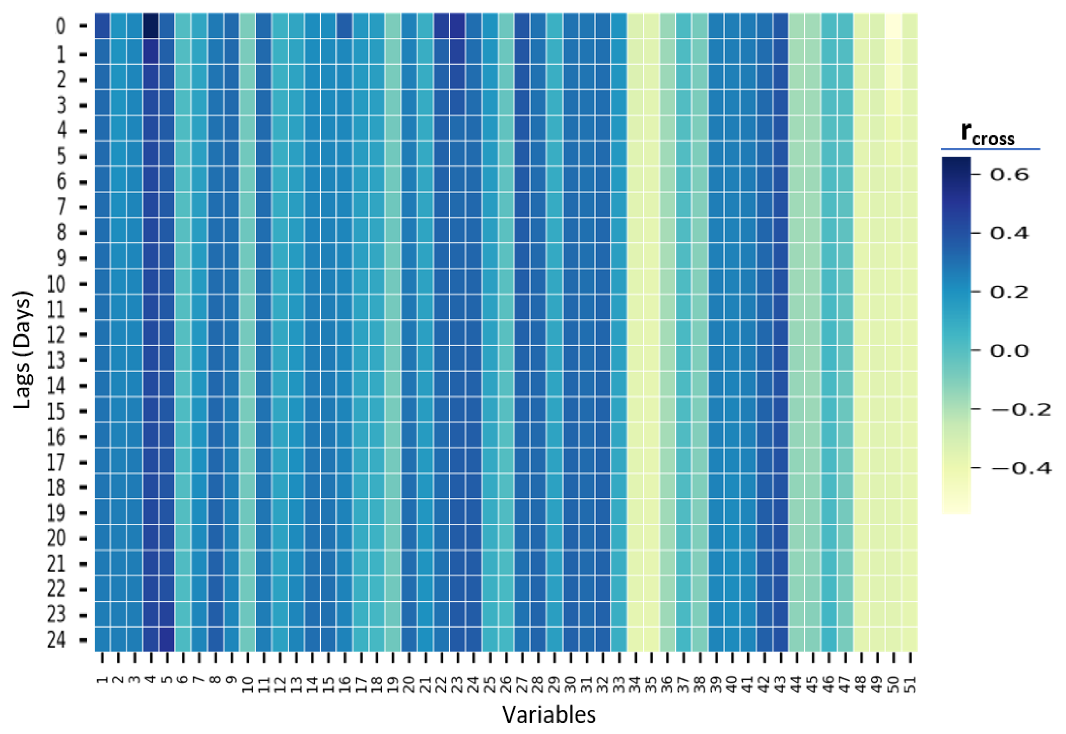
Atmospheric and environmental variables are inter-related and play major roles in sea level variations [19]. When observed data are not available, satellite based data with an associated variable can be effective to estimate trends of environmental variables due to climate change [20,21]. The hydrologically based dataset from GLDAS 2.0 (https://ldas.gsfc.nasa.gov/gldas, accessed on 5 February 2021) is associated with the changes in sea level. This is supported by the results of Ref. [22], which claims that variability in hydrological variables are linked to the sea level change through water held in soil, surface waters and aquifers. The MODIS-Terra and MERA-2 (https://terra.nasa.gov/data/modis-data, accessed on 5 February 2021) dataset variables provide valuable information on atmospheric precipitation, pressure, and temperature. Global warming and sea level changes are directly related as shown by many studies [23,24,25,26]. Studies on predictions of sea level rise have produced many controversial findings and arguments [27,28,29,30] and the studies undertaken confirms that precipitation and temperature have much more of an impact than initially thought on sea level variability. The inclusion of these variables helped to achieve a better fit with observed sea level variation [29]. Figure A1 in Appendix A shows the correlogram to illustrate the covariance between the mean sea level and the predictor variables in terms of cross-correlation for the Fiji Islands. The dark shades indicate a higher cross-correlation value.
A total of 53 predictor variables were extracted from a global pool for data modelling. These are satellite (MODIS, GLDAS-2.0, MODIS TERRA, MERRA-2)-based data. Table A1 in Appendix A describes each of these in more detail. Each predictor variable is correlated with the objective variable to determine the degree of correlation before they are further screened using decomposition and feature selection. Table A2 in Appendix A provides the relevant information on optimum hyperparameters. Using the conventional models, the traditional antecedent lagged matrix of the daily predictors’ variables was applied. The prior application of the NCA feature selection algorithm was made before using CCF and PACF and before significant predictors were removed from the model. NCA was applied to highlight the most pertinent features from the lag in predictors that the antecedent experienced for the hybrid model.

3. Materials and Methods

The mean sea level is the target variable in this study. The dataset for this is obtained from the Bureau of Meteorology (BOM) (Pacific Sea Level and Geodetic Monitoring Project File information and Instructions (bom.gov.au, 10 May 2021)). These are hourly data and measured as observed sea level in meters above the tide gauge zero. The sea level data recording is part of the Pacific and Geodetic monitoring (PSLGM) which comes under the Climate and Oceans Support Program in the Pacific (COSPPac). The selected countries (Fiji, PNG and Marshall Islands) for this study are participating nations in this program. These countries host a permanent tide gauge facility which records the observations on sea levels and tides. Tide gauges are fitted with sensors which record the height of the surrounding water level [31,32]. The design has been improved over the years to protect sensitive electronics, transmitting devices, backup power and storage components. The satellite data is generated using remote sensing technologies such as sensors and radars which collect the measurements [33,34,35].
Firstly, we used the harmonic analysis method for sea level trend observation. The procedure involved fitting the observations with a function using a least-square computation [36,37,38]:
m ( t ) = a 0 + a t t + a cos 1 cos ω 1 t + a sin 1 sin ω 1 t + a cos 2 cos ω 2 t + a sin 2 sin ω 2 t
where t is the sampling interval, ω 1 and ω 2 are the yearly and half-yearly angular frequencies. a 0 ,   a 1   , a 2 ,   a t ,   a cos 1 ,   a sin 1 , a cos 2 and a sin 2 are unknown coefficients that can be estimated through least squares. The sea level residual was assumed to have a zero mean and it follows Gaussian distribution [37,38,39]. The quality of the tide gauge data was screened by the Pope Blunder Test [40] to remove any spurious changes in the data.
The coefficients were used to find the amplitudes of the annual (A):
A = ( a cos 1 ) 2 + ( a sin 1 ) 2
and semi-annual (SA):
S A = ( a cos 2 ) 2 + ( a sin 2 ) 2
The analysis and computation of the large dataset from 1994 to 2020 for the trend and increase in sea level was performed in MATLAB.
Secondly, we combined the Convolutional Neural Network (CNN) and Gated Recurrent Unit (GRU) and developed the hybrid models for MSL forecasting. The standalone models were used for benchmarking the objective model. These were Decision Tress (DT) and Support Vector Regression (SVR). Complete Ensemble Empirical Mode Decomposition with Adaptive Noise (CEEMDAN) was used for input signal decomposition with the machine learning algorithms to further improve the accuracy in forecasting. Feature selection of the predictor inputs was generated by cross-correlation and Neighbourhood Component Analysis (NCA).
It was critical to optimise the objective model’s architecture to incorporate the relationship between predictors and model for the deep learning models. A multi-phase CNN-GRU and GRU models were developed using Python-based deep learning packages of TensorFlow and Keras. Reliable statistical metrics were used to investigate the forecasting robustness of the incorporated models. Deep learning libraries of Keras [41,42] and TensorFlow [43] were used to implement the algorithms for the proposed models. Finally, the matplotlib [44] and seaborn [45] packages were used to visualise the forecasted MSL. Three methods for selecting lagged memories of MSL and predictors for an optimal model are used in this study. These include the Auto Correlation Function (ACF), Partial Auto Correlation Function (PACF) and the cross-correlation function (CCF). PACF was specifically used to determine significant antecedent behaviour in terms of the lag of MSL [46,47].
Figure 2 shows the decomposed intrinsic mode functions (IMFs) and residual of MSL variable. Complete Ensemble Empirical Mode Decomposition with Adaptive Noise (CEEMDAN) is an improved algorithm of Empirical Mode Decomposition (EMD) and Ensemble Empirical Model Decomposition (EEMD). It can adaptively decompose signals into IMFs in order. CEEMDAN algorithms effectively analyse nonlinear and non-stationary signals. EMD and its variant algorithms have been applied to many data modelling studies [10,48,49].
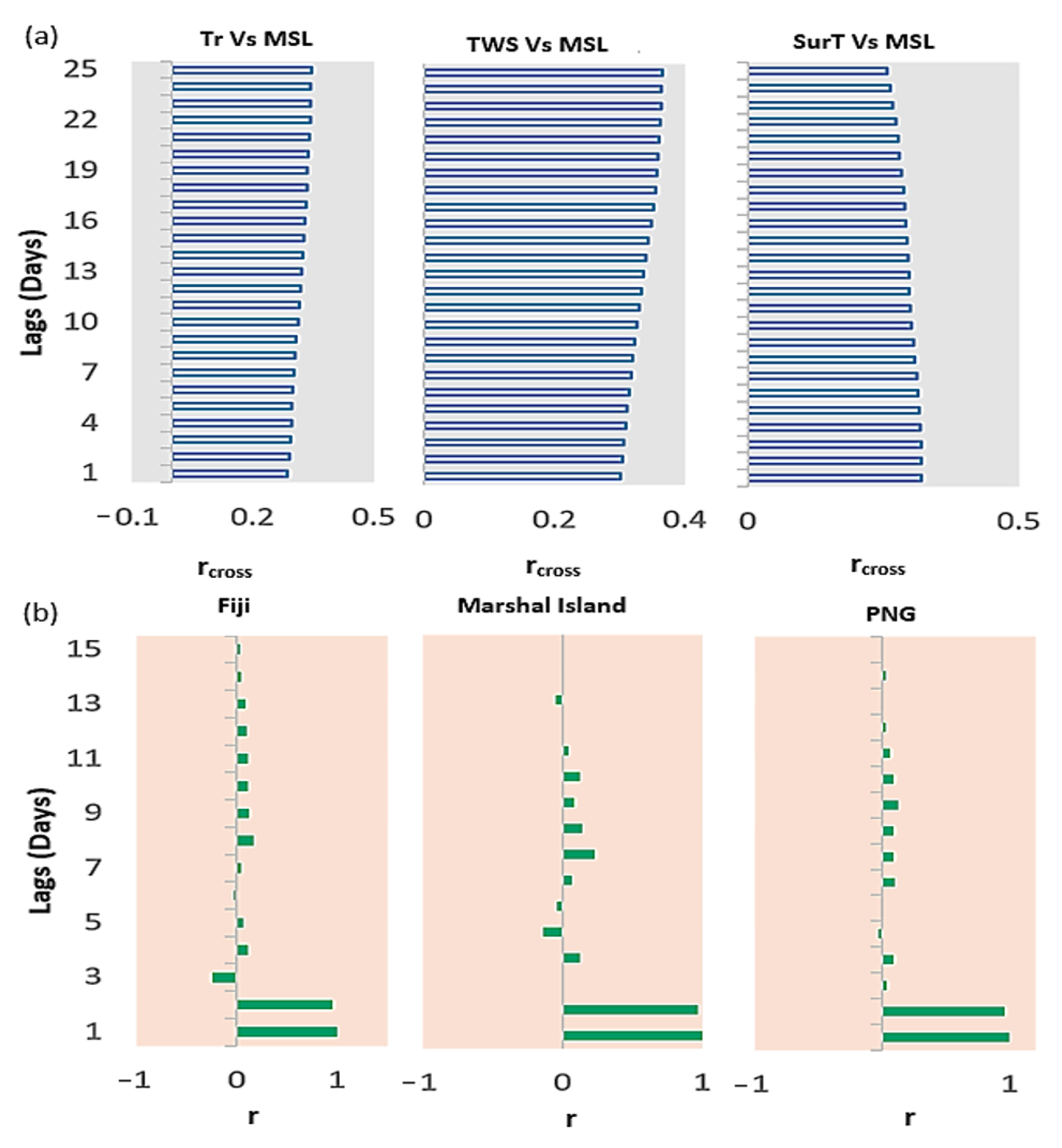
The cross-correlation function selected the input signal pattern based on the predictors’ antecedent lag [50] and determined the predictors’ statistical similarity to the target variable. Antecedent daily delays are shown in Figure 3.
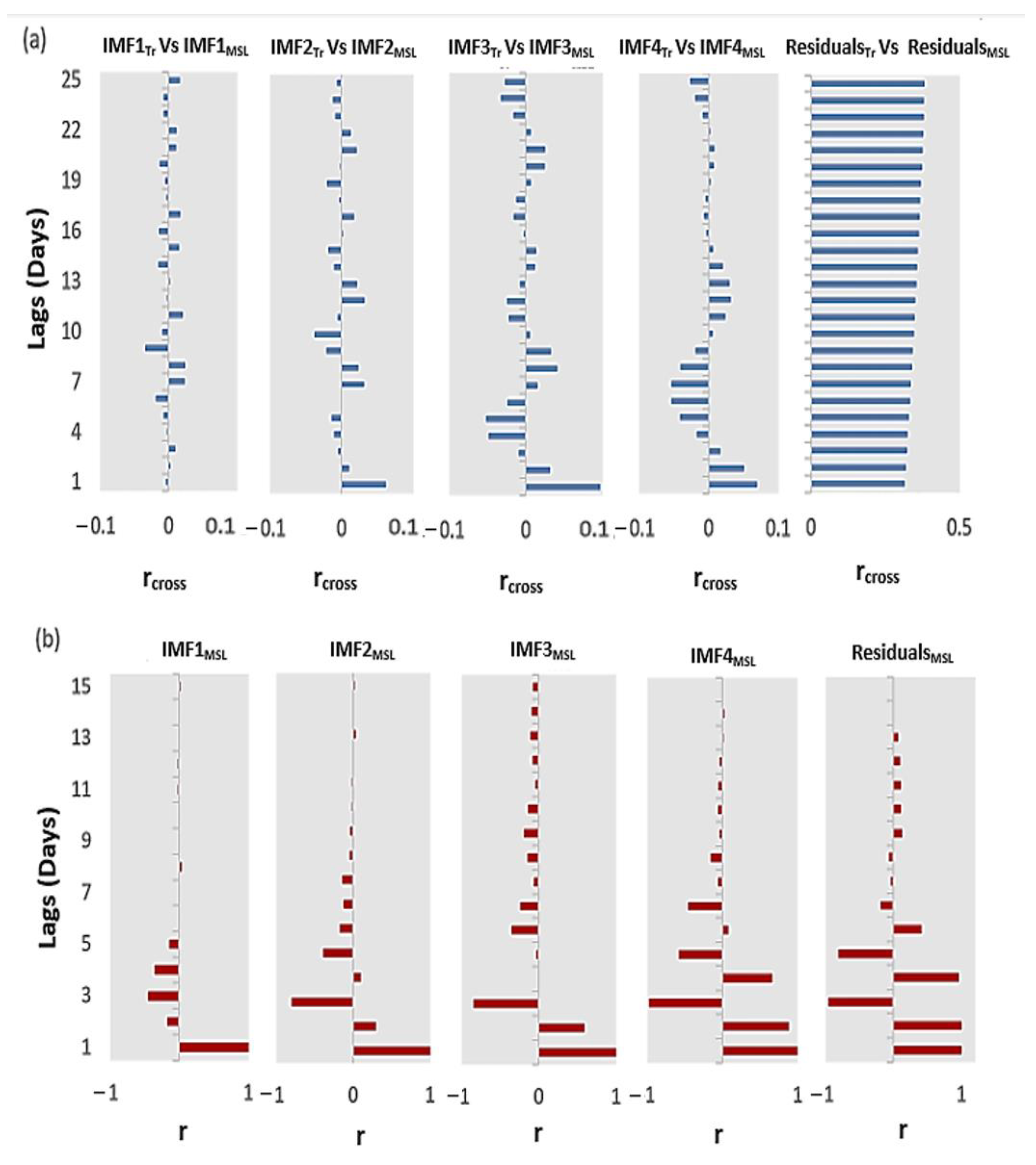
A set of significant input combinations were determined by evaluating each predictor’s rcross with MSL. As shown in Figure 4, the highest correlation between the data and MSL was found for all stations at lag zero (rcross 0.22 to 0.75). For Tr and TWS, both demonstrated significant rcross from 0.25 to 0.40 and 0.30 to 0.38, respectively. To increase the predictors’ diversity, some predictors with insignificant lags such as Cloud Top Pressure (CP), Cloud Top Temperature (CTm), and Snow evaporation (Sn) were also considered. These lags were screened by the NCA process before MSL prediction.
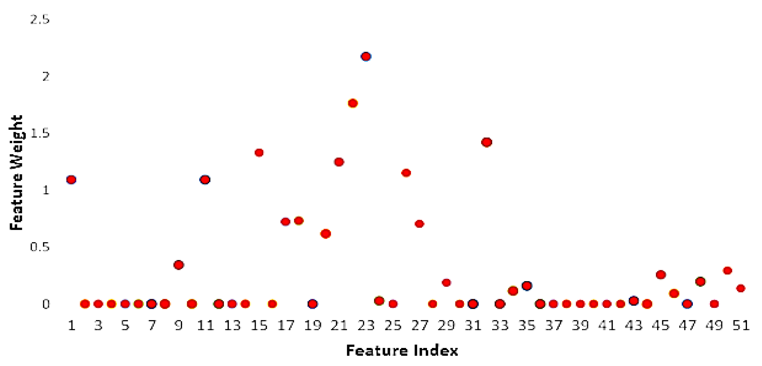
The strategy for selecting lags from the cross-correlation function for all sites are identical to what is used for the Fiji Islands. Figure 5 shows the graph of feature index and feature weight for the case of Fiji Island using the NCA method. NCA is a non-parametric feature selection method that helps maximise the prediction accuracy [51,52] and reduce the computational load by selecting the significant inputs. The weights of the irrelevant features are zero as shown in Figure 5. The algorithm is performed in MATLAB by fsrnca function for regression using the predictors. The function, fsrnca learns the feature weights by a diagonal adaptation of Neighbourhood Component Analysis with regularisation.
The predictor variable data sets are normalised between 0 and 1 to minimise the overestimation of one variable to another.
A n o r m = A A m i n A m a x A m i n
In Equation (4), A is the respective predictor, A m i n is the minimum value for the predictor, A m a x is the maximum value of the data and A n o r m is the normalised value of the data. After normalising the predictor variables, the data sets were partitioned as follows: 70% of the data sets for training, 15% of the data for testing, and the remaining 15% of the data were used for validation as shown in Table 2.
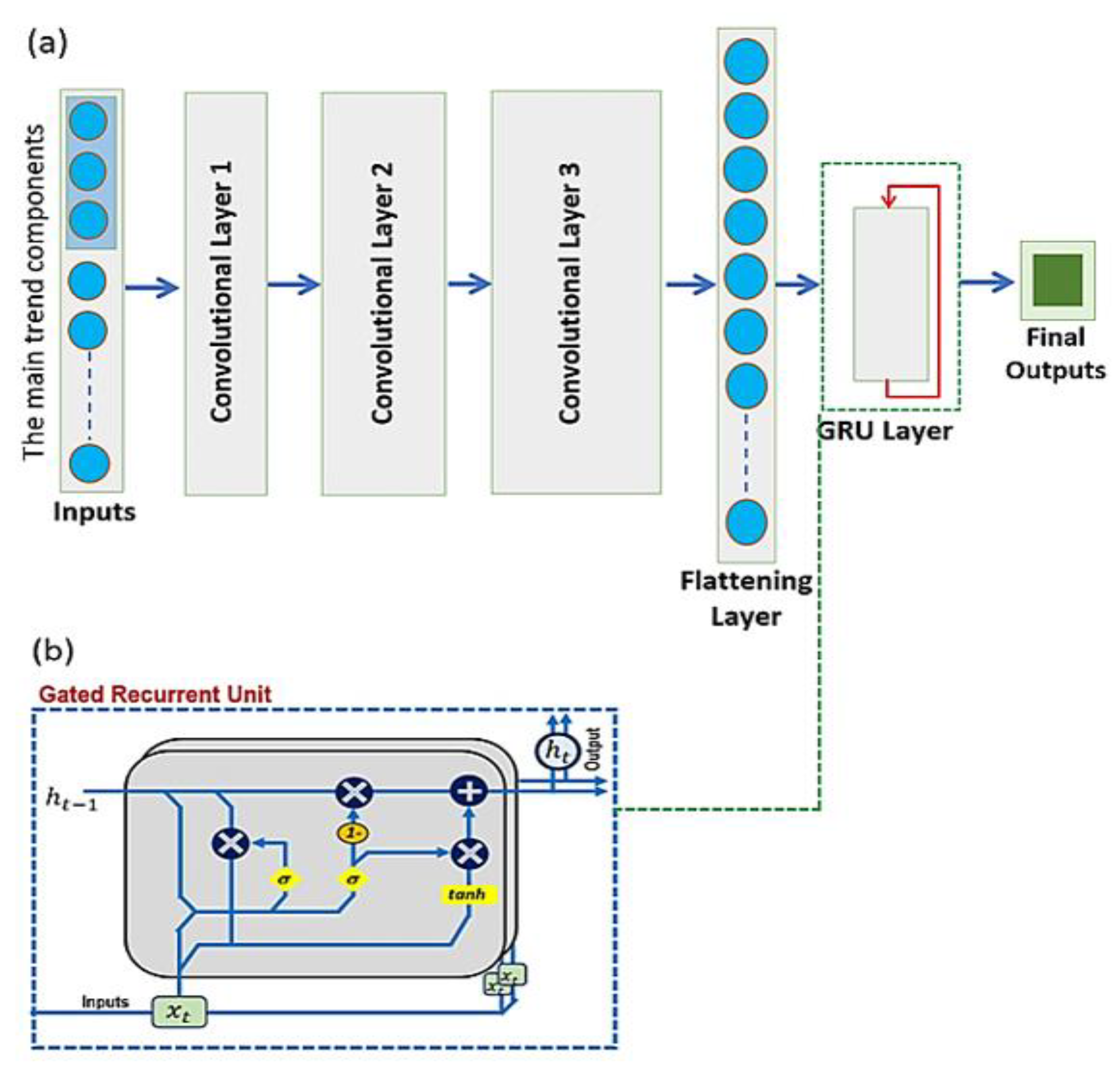
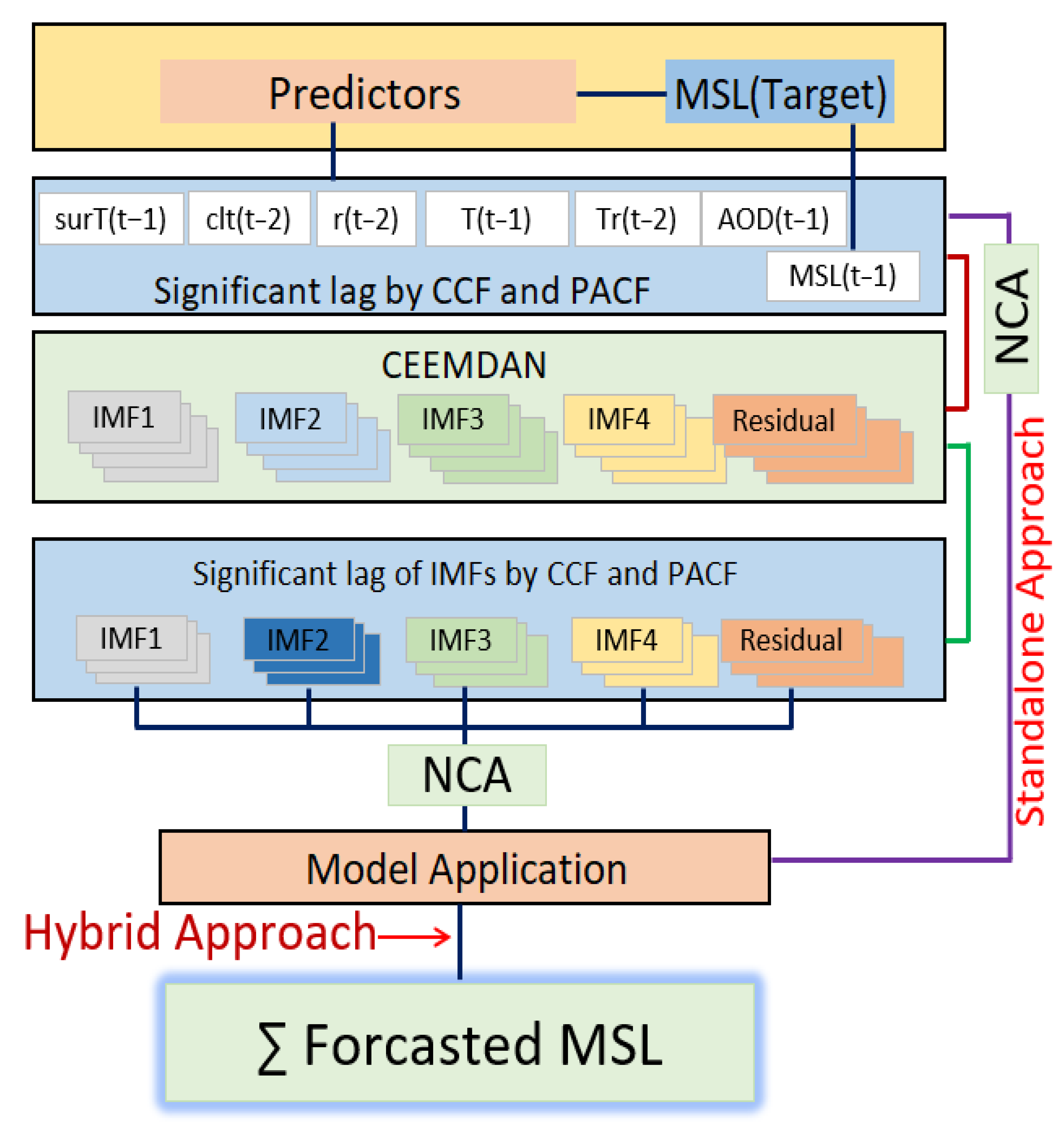
The GRU model was followed by the development of a hybrid GRU model with 3-layered CNN and 3-layered GRU, as illustrated in Figure 6. Note: ( x t is the new input, h t is the hidden state, h t 1 is the last hidden state, C ˜ t is the cell state, C ˜ t 1 is the previous cell state, t a n h is the hyperbolic tangent function, O t is the output gate and σ is the logistic sigmoid function). The overall modelling process is shown in Figure 7. The predictors and MSL target variable pass through the CEEMDAN algorithm for IMF breakdown whereby significant lags were selected by the NCA feature selection as the significant model inputs. This was carried out for both hybrid and standalone models.

4. Results

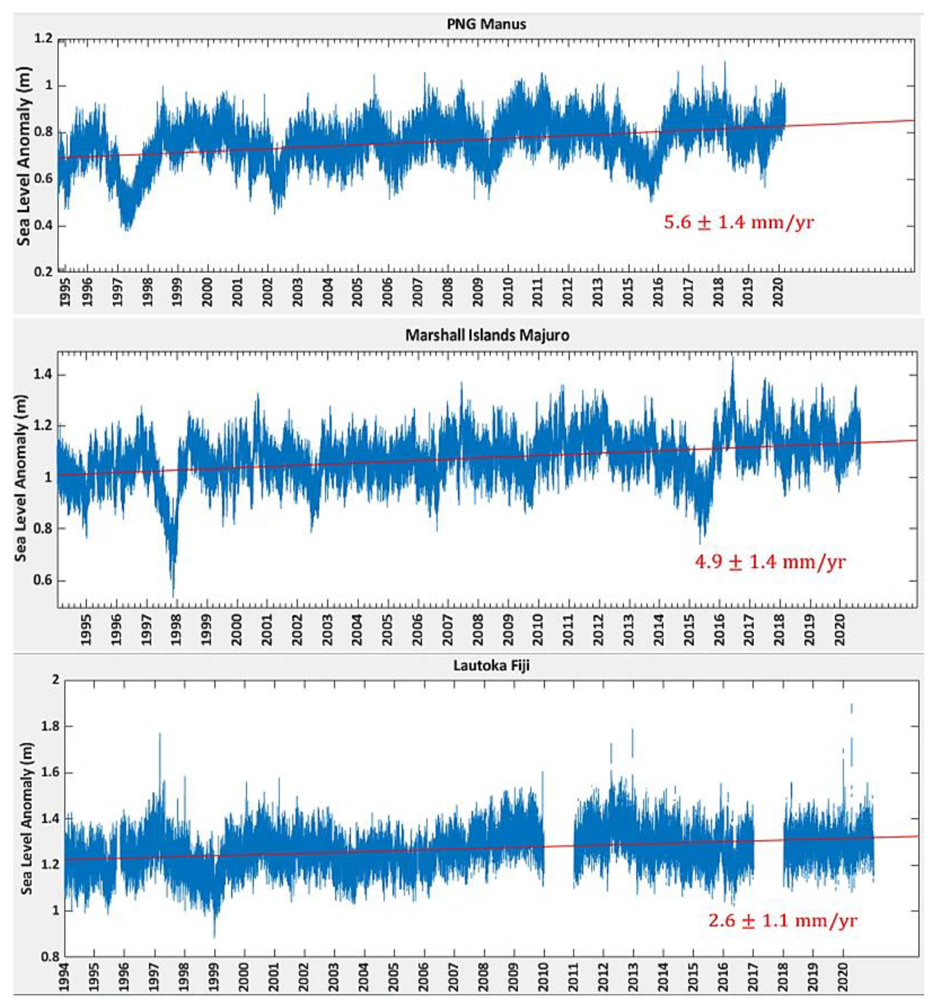
This section presents the results of the sea level trend analysis and the performance of the proposed hybrid deep learning (i.e., CEEMDAN-CNN-GRU), benchmark hybrid (i.e., CEEMDAN-GRU, CEEMDAN-SVR, CNN-GRU), and the standalone models (GRU, DT and SVR). The tables and figures demonstrate substantial information obtained from the trend and deep learning forecasting of MSL. Figure 8 shows the trend of the MSL increase for the past 26 years. The trends shown in these figures with error uncertainty agree with what was obtained in Ref. [53] for the rate of Black Sea level increase over 100 years, which is 3 mm/yr on average for all stations of the northern coast of the Black Sea. This estimate also agrees with the studies in [54,55,56,57] whereby it is also claimed that the global average sea level has been rising by about 3 mm a year.
The models were evaluated based on the testing dataset using eight statistical metrics from Equations (5)–(11) of the predicted results. The models were evaluated by comparing the model predictions to the observed data.
  • Correlation Coefficient (r)
    r = [ i = 1 n ( D O i M D O ) ( D S i M D S ) i = 1 n ( D O i M D O ) 2 i = 1 n ( D S i M D S ) 2   ] 2
  • Nash–Sutcliffe Coefficient (NS)
    N S = 1 [ i = 1 n ( D O i D S i ) 2 i = 1 n ( D O i M D O ) 2 ] , N S 1
  • Legates and McCabe index (LM)
    L M = 1 [ i = 1 n | ( D S i D O i ) |                 i = 1 n | D O i M D S |   ] ,   0 L 1
  • Willmott’s Index of agreement (d)
    d = 1 [ i = 1 n ( D O i D S i ) 2 i = 1 n ( | D S i M D O | + | D O i M D S | ) 2 ]
  • Root Mean Square Error (RMSE)
    R M S E = ( 1 n ) i = 1 n ( D S i D O i ) 2  
  • Mean Absolute Error (MAE)
    M A E = 1 n i = 1 n | ( D S i D O i ) |
  • Root Mean Absolute Error (RMAE)
    M A E = 1 n i = 1 n | ( D S i D O i ) | 1 n i = 1 n | ( D O i ) |
  • Relative Root Mean Square Error (RRMSE)
    R R M S E = ( 1 n ) i = 1 n ( D S i D O i ) 2 1 n i = 1 n D O i × 100
    w h e r e :   D O i O b s e r v e d   d a t a ,   D S i S i m u l a t e d   d a t a ,   M D O i O b s e r v e d   d a t a ,   M D S i M e a n   S i m u l a t e d   d a t a
Correlation coefficient (r) analysis is widely used to determine the relationship between two different variables [58]. It also indicates the strength or the degree of association between the considered variables. In this case, the observed and predicted values from the test dataset. Nash–Sutcliffe (NS) [59] is used to determine model accuracy and assess the goodness of fit [60,61]. The Wilmott Index (d) or index of agreement developed by Wilmott [62] is a standardised measure of the degree of model prediction error. It represents the ratio of the mean square error and the potential error with the ability to detect additive and proportional differences in the means and variances of observed and predicted datasets [63]. Equations (9)–(11) are used to compute error values between the observed and predicted mean sea level values. The eight evaluation metrics provide a reliable means of comparison. Table 3 compares the hybrid deep learning models (i.e., CEEMDAN-CNN-GRU) to their respective standalone models in terms of the statistical metrics r, NS, RMSE, RMAE and MAE.

5. Discussion

Firstly, the harmonic analysis of the mean sea level trend showed an estimated increase of 5.6 mm/yr for PNG, 4.9 mm/yr for the Marshall Islands and 2.6 mm/yr for Fiji. For an estimated 20-year period, this is a considerable rise, 112 mm for PNG, 98 mm for Marshall Island and 52 mm for Fiji. According to a fourth assessment report [64], the rate of global average sea level rise has risen from 1.8 mm/yr to 3.1 mm/yr from 1961 to 1993. Given most settlements in these small islands are around the coastal areas, and taking into account that the land slope in the coastal zone is usually relatively small, ~1/10 or even less, this rise has caused many problems for people in these areas [65]. The major effects of sea level rise include loss of land, coastal erosion and flooding [66,67].
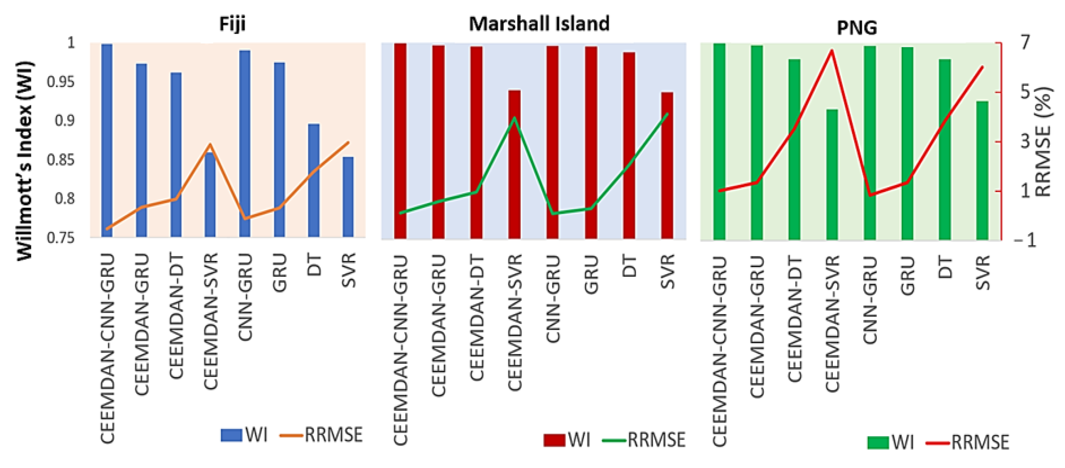
Secondly, the developed CEEMDAN-CNN-GRU prediction model implemented for the testing phase captures high values of correlation coefficient (r), Nash–Sutcliffe efficiency (NS), Willmott’s Index (WI), and notable lower values of root mean square error (RMSE), mean absolute error (MAE) and Relative Root Mean Square Error. The highest performance value was recorded for the station in Fiji by the CEEMDAN-CNN-GRU model, r (0.996), RMSE (0.004), NS (0.993), MAE (0.003) and RMAE (0.239) comparing with CEEMDAN-GRU (r = 0.959, NS = 0.907 and RMAE = 0.844%) and CNN-GRU (r = 0.982, NS = 0.964 and RMAE = 0.513%) models. The standalone models (i.e., SVR and DT) were outperformed by the single deep learning and hybrid deep learning models. However, the hybrid DT model (CEEMDAN-DT) showed a better performance, obtaining a value of r = 0.927, NS = 0.850 and RMAE = 1.075%. The CEEMDAN-CNN-GRU model with other two stations (i.e., Marshal Island and PNG) also showed the respective superior performance, with values of r (0.995–0.996), NS (0.989–0.991), RMSE (0.007–0.010) and RMAE (0.650–0.628%). The performance metrics of this model are followed by the CNN-GRU, CEEMDAN-GRU and GRU model accordingly. The proposed hybrid deep learning (i.e., CEEMDAN-CNN-GRU) was further assessed based on Willmott’s Index (WI) and RRMSE for all tested models, as shown in Figure 9.
Figure 9 shows the low magnitude of RRMSE and high magnitude of WI for the objective model at the three monitoring stations. The RRMSE value between 6.8% to 7% is far better than the other associated benchmark models, while the WI value ranges from 0.993 to 0.996. Additionally, the Marshall Island and PNG stations also show better WI value for CEEMDAN-GRU and CNN-GRU models.
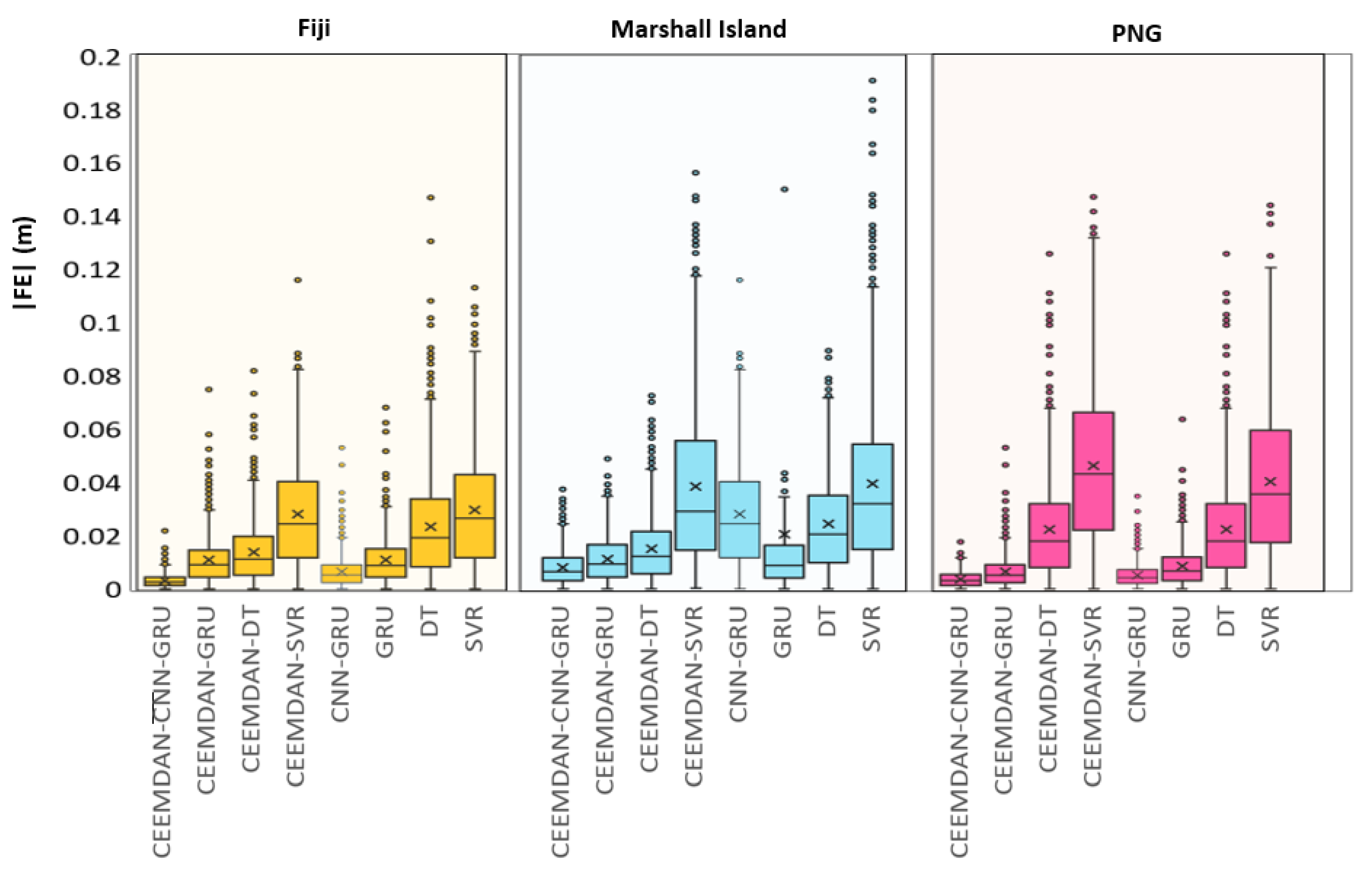
With further analysis through box plot, the forecasted-to-observed MSL and absolute forecasting errors of all hybrid models (CEEMDAN-CNN-GRU, CEEMDAN-GRU and CNN-GRU) for three stations are shown in Figure 10. The dispersion of the absolute forecasted error (|FE| = MSLfor − MSLobs) depicts the amount of maximum error. Figure 10 illustrates the data by quartiles to show the distinct outliers. The plot is precisely situated between the 25th percentile and the 75th percentile. The CEEMDAN-CNN-GRU provides a closed distribution of error values for Fiji and PNG stations. The lower end of the plot for |FE| is situated within the lower quartile and upper quartile. Furthermore, the CNN-GRU model shows comparable prediction when applied to both locations. The error dispersion of Marshall Island was found to be higher when compared with the other two stations. More analysis of the absolute forecasted error (|FE|) from the hybrid CEEMDAN-GRU-GRU model further confirms the suitability of the hybrid GRU approach in forecasting the MSL of three selected Pacific islands with the narrowest distribution.
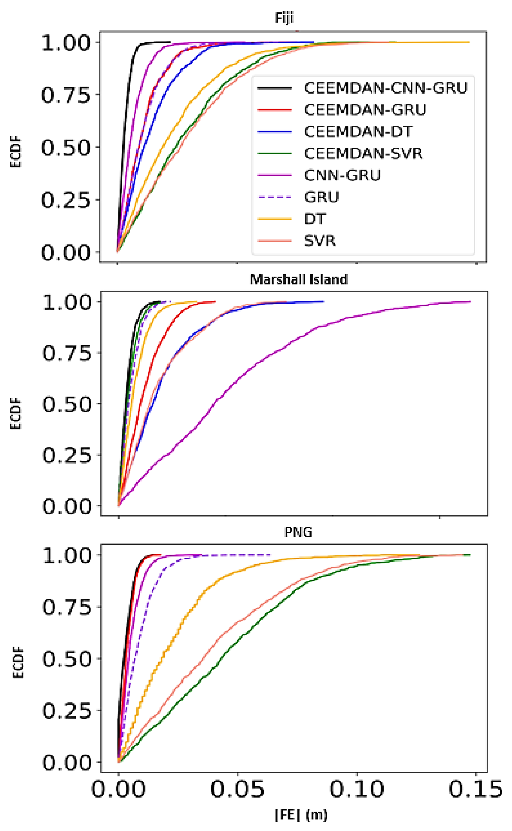
We have also used empirical cumulative distribution functions (ECDF) of absolute forecast error (|FE|) to further evaluate the objective model. Figure 11 at Fiji station indicates that 95% of the results from the CEEMDAN-CNN-GRU model fall within the 0.01 m error bracket, followed by a considerably larger error associated with CNN-GRU (0.025 m), GRU (0.05 m) and the RF model (0.06 m). Similar performance was found for the other stations as well. The objective model was favoured by predictions ranging between the 95th and 98th percentile, which was the best for the current forecast.
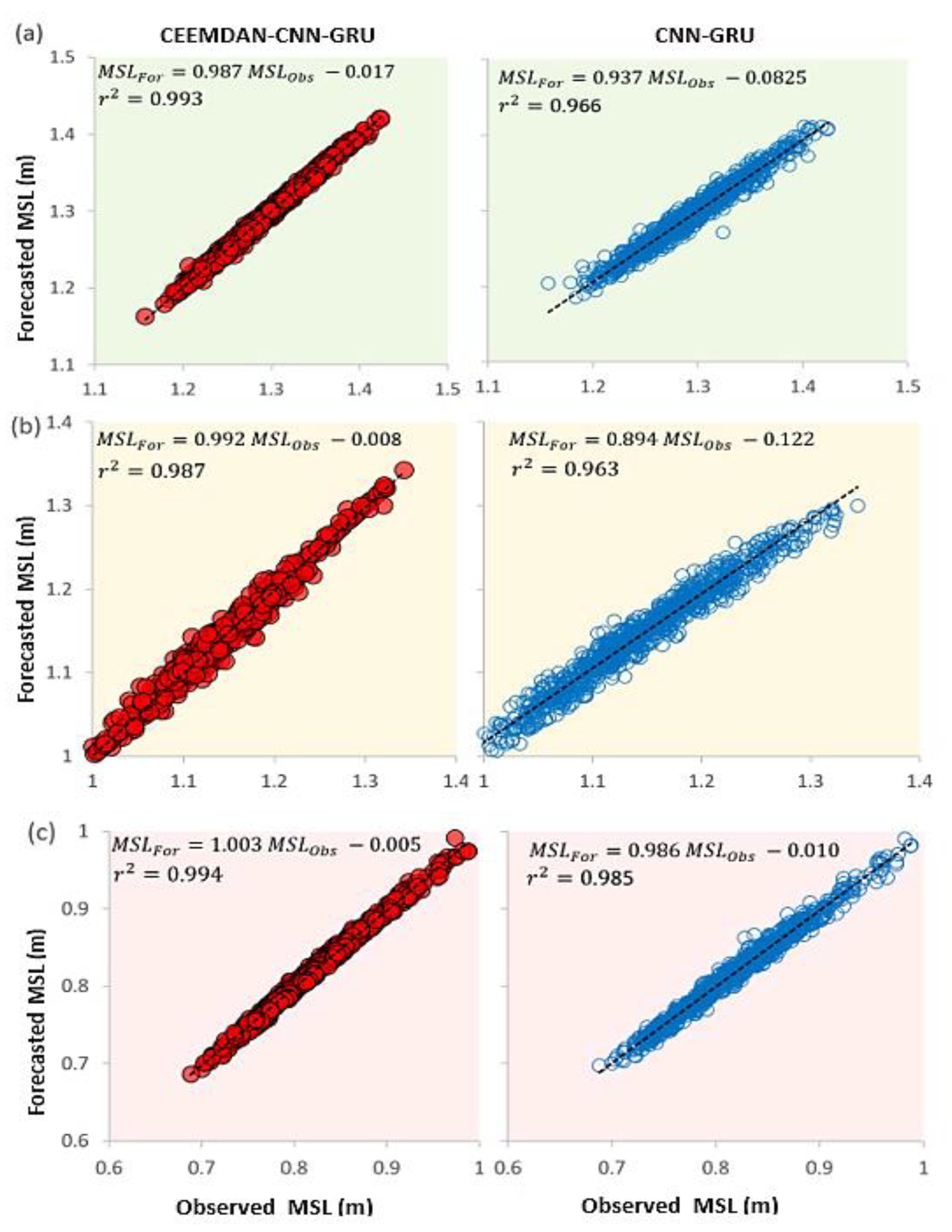
Next, the scatterplot of the forecasted (MSLfor) and observed (MSLobs) MSL for three stations using eight models show a precise comparison of MSL forecasting (Figure 12). The scatter plots show the coefficient of determination (r2) with goodness-of-fit between predicted vs. observed MSL and a least-square fitting line with the corresponding equation; MSLfor = (mxMSLobs) + C, where ‘m’ is referred to as the gradient, and ‘C’ is denoted as the y-intercept. Figure 12 shows that the proposed model displays significant performance with a higher r2 value. The MSL forecasting using the objective model (i.e., CEEMDAN-CNN-GRU) for the PNG station performed better than the other stations and models. The magnitudes registered from the hybrid CEEMDAN-CNN-GRU model for three stations were the closest to unity, which, in pairs (m|r2), are 1.003|0.994 for PNG, followed by Fiji Island (0.993|0.987) and Marshall Island (0.992|0.987). Moreover, the CNN-GRU model provided a comparatively better pair, such as 0.986|0.985 for PNG, 0.937|0.966 for Fiji and 0.894|0.963 islands, accordingly. Alternatively, the y-intercepts [ideal value = 0] were found to be closer to zero, i.e., 0.005 (PNG), 0.008 (Marshall Island) and 0.017 (Fiji).
In terms of accuracy, the hybrid deep learning model (i.e., CEEMDAN-CNN-GRU) confirmed the MSL forecasting model’s superiority as shown in Table 4.
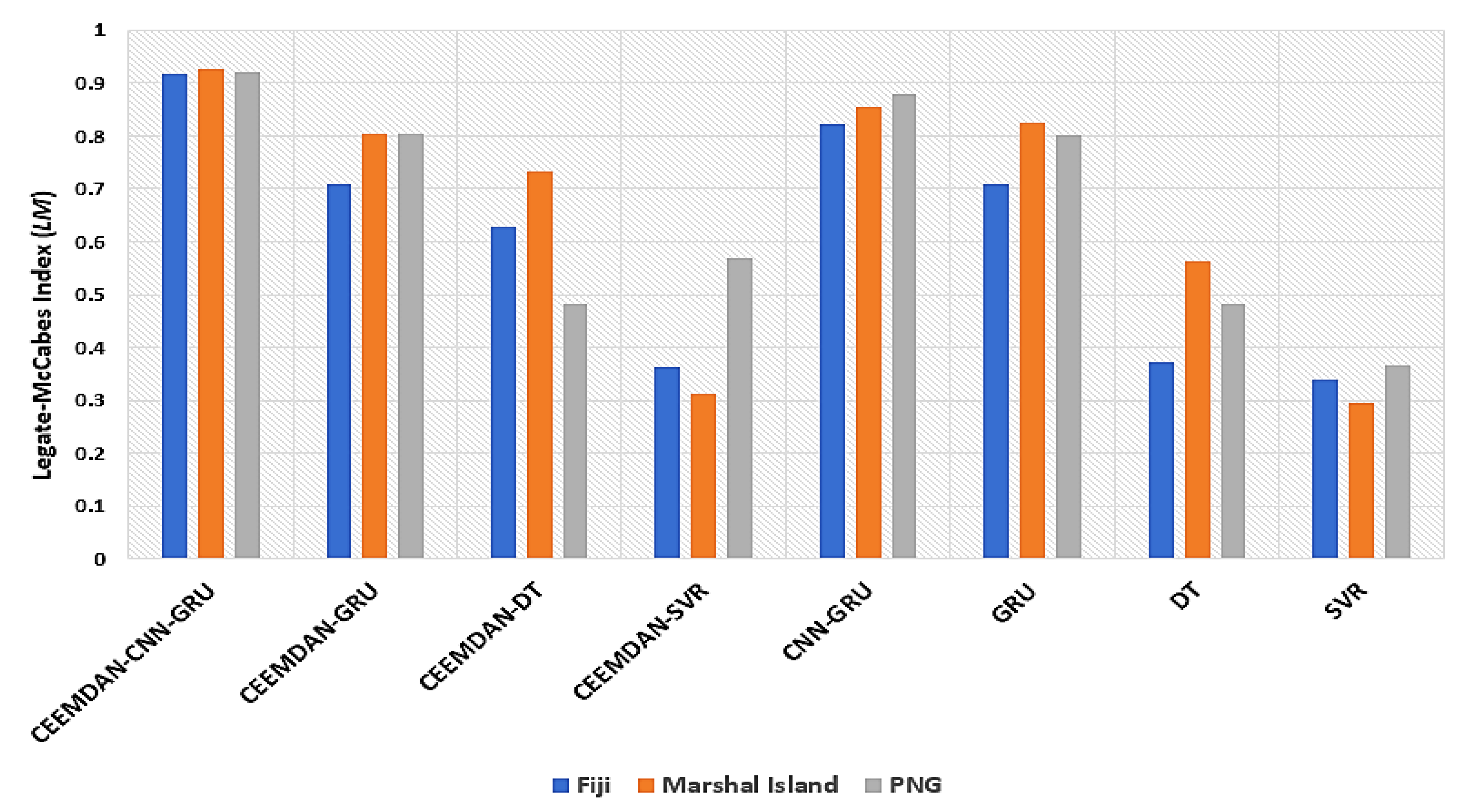
When values tend to be high, the Legates and McCabe Index (0 ≤ LM ≤ 1.0) offers an advantage over WI as outliers can increase the value of WI. It is also noted that the LM value of GRU is higher than the CEEMDAN-SVR/DT value which can happen due to redundancy in the input data. Figure 13 shows the visualisation of LM values of the hybrid deep learning approach (i.e., CEEMDAN–CNN-GRU), the benchmark models (i.e., CEEMDAN-GRU, CNN-GRU, and CEEMDAN-DT, etc.) and standalone models (GRU, DT and SVR) for the three Pacific Island countries. For the hybrid deep learning model, the LM index indicates a notably better result. Figure 12 shows that for PNG, the maximum value of LM was 0.927, and the least value was 0.917 for Fiji Island. The CEEMDAN-CNN-GRU model ranges from 0.916 to 0.927, while the CNN-GRU model’s range is 0.821 to 0.878. The standalone models (GRU, DT, and SVR) show lower LM values than the hybrid deep learning models. Combining the feature extraction algorithm (i.e., CEEMDAN) and feature selection algorithm (i.e., NCA) with significant lags with the CNN-GRU model significantly improves MSL for the Pacific islands. However, the hybrid DL models have a high computational cost when compared to standalone models. The numerical simulations take more time as it needs to be processed through three different algorithms (CEEMDAN-CNN-GRU).
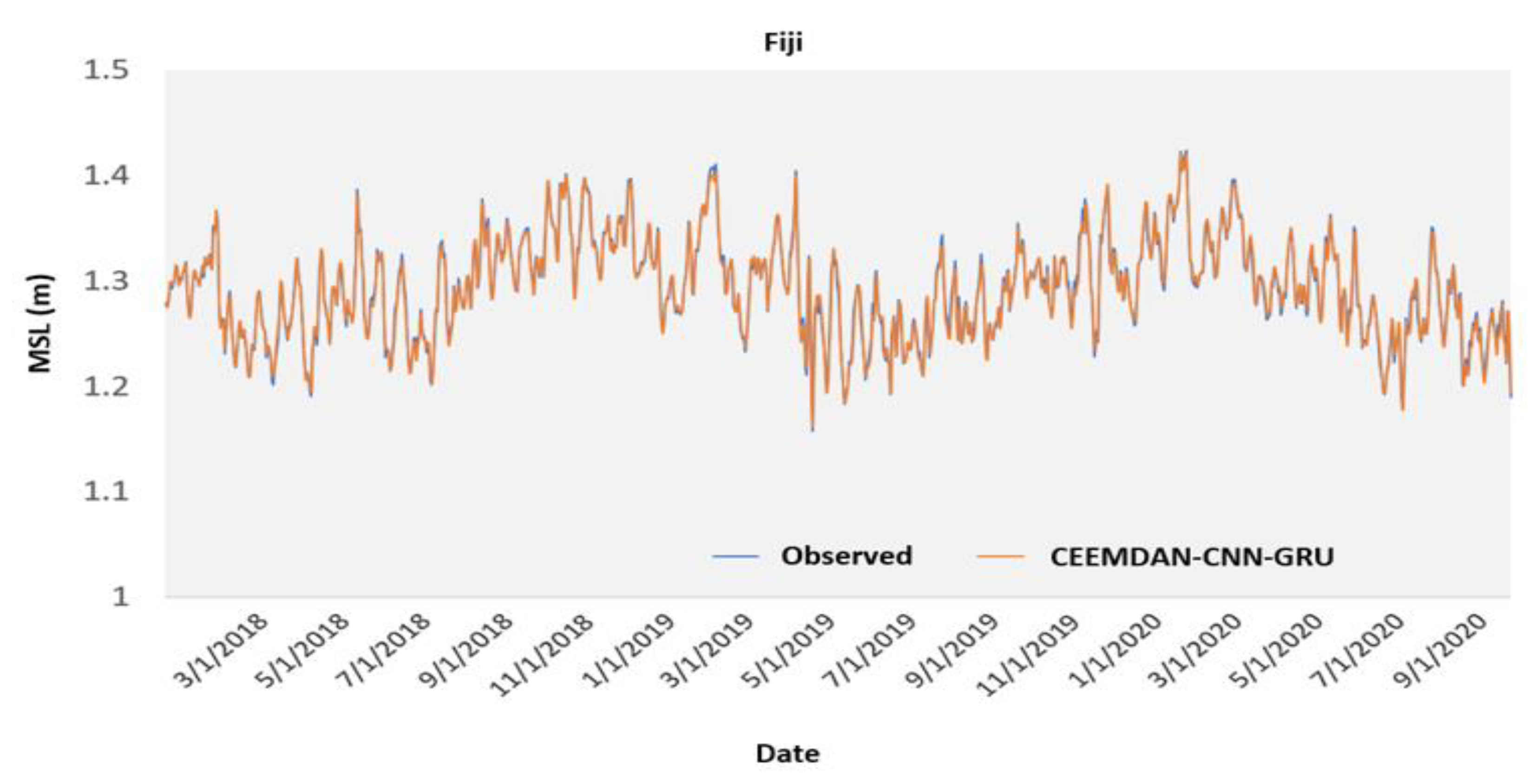
Time series plots were used to understand forecasting ability and the comparison between standalone and hybrid models. Figure 14 represents the forecasted and observed MSL time series plot. It shows the forecasted and observed MSL of the Fiji station with CEEMDAN-CNN-GRU. The research results indicate that the proposed CEEMDAN-CNN-GRU model is closer to the observed MSL. The application of the NCA and CEEMDAN algorithm showed notable MSL improvement.

6. Conclusions

To study the effectiveness of aggregated significant antecedent satellite-driven variables and tide gauge mean sea level data, this study has successfully implemented a trend assessment to determine the mean sea level rise from 1994 to 2020 and forecasted daily mean sea level (MSL) for three Pacific Island States. Firstly, the harmonic trend analysis has shown an increase in the past 26 years. This increase is significant and coincides with the global trend on sea level rise with climate change. This study can help to estimate what the rise might be in the next decade in these small islands and will be very useful for stakeholders in planning and taking important decisions on adaptation strategies.
Secondly, artificial intelligence models can also use climate and environment variables can also be used to forecast the mean sea level values as shown for the testing phase in this study. The NCA feature selection algorithm was able to screen the crucial features of the study’s dataset to optimise the predictor inputs. The findings have shown superior performance by the objective model of CEEMDAN-CNN-GRU for each station when compared to all other benchmark models. NCA feature selection algorithm has shown to be an effective option for extracting the useful features of the predictors. It should be noted that the hybrid models do have a high computational cost as the data inputs are processed through more than one modelling platform. The performance metrics show that the NCA and CEEMDAN-optimised models had better performance and higher efficiency metrics (i.e., r, NS, and WI) and lower error metrics (i.e., MSE and RMSE). In MSL forecasting, the performance of the standalone models (GRU, DT and SVR) was poor when compared to the hybrid models. GRU performed better on three stations among the standalone models, with correlation coefficients ranging from 0.955 to 0.984. The proposed harmonic mean sea level trend analysis and DL hybrid model can also be used for other Pacific Island counties for MSL forecasting.

Author Contributions

Conceptualisation, N.R. and Z.G.; methodology, N.R.; software, N.R., A.A.M.A.; validation, N.R.; formal analysis, N.R.; investigation, N.R., Z.G., Y.S., A.A.M.A.; resources, N.R., A.A.M.A.; data curation, A.A.M.A., writing—original draft preparation, N.R., Z.G., Y.S., A.A.M.A.; writing—review and editing, N.R., Z.G., Y.S., A.A.M.A.; visualisation, N.R., A.A.M.A.; supervision, N.R.; project administration, N.R.; funding acquisition, N.R., Z.G., Y.S. All authors have read and agreed to the published version of the manuscript.

Funding

This research was funded by the Faculty Collaboration Grant, University of Southern Queensland (USQ). Y.S. acknowledges the funding of this study provided by the grant No. FSWE-2020-0007 through the State Task Programme in the Sphere of Scientific Activity of the Ministry of Science and Higher Education of the Russian Federation and the funding provided by Grant of President of the Russian Federation for the state support of Leading Scientific Schools of the Russian Federation (grant No. NSH-70.2022.1.5).

Data Availability Statement

Publicly available datasets were analysed in this study. The data can be found here: Pacific Sea Level and Geodetic Monitoring Project File information and Instructions (bom.gov.au, 10/30 May 2021).

Conflicts of Interest

The authors declare no conflict of interest.

Abbreviations

MSLMean Sea Level
CEEMDANComplete Ensemble Empirical Mode Decomposition with Adaptive Noise
GRUGated Recurrent Unit
CNNConvolutional Neural Network
DLDeep Learning (DL)
NCANeighbourhood Component Analysis
BOMBureau of Mereology
ACFAuto Correlation Function
PACFPartial Auto Correlation Function
CCFCross-Correlation Function
rCorrelation Coefficient
NSNash–Sutcliffe Coefficient
LLegates and McCabe Index

Appendix A

Appendix A.1. Figures

Figure A1. Correlogram showing the covariance between the objective variable (MSL) and the predictor variables in terms of the cross-correlation coefficient (rcross) for Fiji Islands for the lags between 0 and 24.
Remotesensing 14 00986 g0a1

Appendix A.2. Tables

Table A1. Description of the global pool of 53 predictor variables used to design and evaluate the hybrid CEEMDAN-CNN-GRU predictive model for mean sea level forecasting.
Variable IDDescription of VariablesAcronymsUnits
Model: GLDAS 2.0
1Average Surface Skin temperature SurTK
2Plant canopy surface waterPkg m−2 s−1
3Canopy water evaporationCwkg m−2 s−1
4Direct evaporation from bare soil EvW m−2
5Snow evaporationSnW m−2
6EvapotranspirationEvpW m−2
7Ground water storageGWSW m−2
8Net long-wave radiation fluxLwkg m−2 s−1
9Ground heat fluxGhm
10Sensible heat net fluxShK
11Latent heat net flux Latkg m−2
12Baseflow-groundwater runoff BgW m−2
13Snow melt daily 0.25 Snmkg m−2 s−1
14Storm surface runoff SSRkg m−2 s−1
15Snow depth daily Skg m−2
16Snow surface temperature Stkg m−2 s−1
17Profile soil moisture PSMkg m−2
18Root zone soil moisture Sznkg m−2
19Surface soil moisture Ssmkg m−2
20Snow depth water equivalent Sdwkg m−2 s−1
21Net short-wave radiation flux Swrkg m−2 s−1
22Transpiration Trmm
23Terrestrial water storage TWSmm
Model: MODIS-Terra
24Aerosol optical depth 550 nm (Dark Target)AOD-
25Scattering angle: mean of daily meanSdegrees
26Combined dark target and deep blue AOD at 0.55 µ for land C-
27Precipitable water vapor 440 to 10 mb: Meanrcm
28Precipitable water vapor surface to 680 mb rwcm
29Precipitable water vapor total col: Mean of level-3 QA weighted rvpcm
30Cirrus reflectance: Daily meanCr-
31Ice Cloud Effective Particle Radius: Daily meanIce-
32Liquid Water Cloud Effective Particle Radius: Daily meanLW-
33Cloud Fraction from Cloud Mask: Day MeanCF-
34Cloud Fraction from Cloud Mask: MeanCFm-
35Cloud Fraction from Cloud Mask: Night MeanCnm-
36Combined Cloud Optical Thickness: Mean CC-
37Ice Cloud Optical Thickness: Mean ICmicrons
38Liquid Water Cloud Optical Thickness: Mean Lmmicrons
39Cloud Top Pressure (Day): MeanCPhPa
40Cloud Top Pressure: MeanCPmhPa
41Cloud Top Pressure (Night): Mean CPnmhPa
42Cloud Top Temperature: Mean CTmK
43Cloud Top Temperature (Day): Mean CTdmK
44Cloud Top Temperature (Night): Mean CTnmK
45Ice Cloud Water Path: Mean ICg/m2
46Liquid Water Cloud Water Path: MeanLQg/m2
47Aerosol Optical Depth 550 nm (Deep Blue, Land-only)A550-
48Deep Blue Angstrom Exponent for land (0.412–0.47µ): MeanD-
49Water vapor near-infrared—clear column (bright land and ocean sunlight only)Wvicm
50Water vapor near infrared—cloudy column: Mean Wvmcm
Model: MERRA-2
512 m air temperature—daily max TmaxK
522 m air temperature—daily mean TrK
532 m air temperature—daily min TminK
Objective Variable
54Mean sea levelMSLm
Table A2. (a) The full range of tested hyperparameters in designing the hybrid CNN-GRU and the GRU predictive model through an extensive grid search process. (b) Optimally selected hyperparameters. ReLU stands for Rectified Linear Units, SGD stands for stochastic gradient descent optimiser.
ModelModel Hyper-Parameter NamesSearch Space for Optimal Hyper-Parameters
(a) Tested Range of Model Hyper-Parameters
CNN-GRUFilter 1[70, 80, 100, 150]
Filter 2[70, 80, 100, 150]
Filter 3[70, 80, 100, 150]
GRU Cell Units [40, 50, 70, 80, 100, 150]
Epochs[500, 800, 1000]
Activation function [ReLU]
Optimiser [Adam], [SGD]
Batch Size[5, 10, 20, 50, 100]
GRUGRU Cell1[70, 80, 100, 110]
GRU Cell 2[70, 80, 100,150, 200, 210]
Epochs[500, 800, 1000]
Activation function [ReLU]
Optimiser [Adam], [SGD]
Batch Size[5, 10, 20, 50, 100]
(b) Optimally Selected Hyper-parameters
CNN-GRUConvolution Layer 1 (C1)80
C1- Activation functionReLU
C1-Pooling Size1
Convolution Layer 2 (C2)70
C2- Activation functionReLU
C2-Pooling Size1
Convolution Layer 3 (C3)80
C3- Activation functionReLU
C3-Pooling Size1
GRU Layer 1 (L1) 200
L1- Activation functionReLU
GRU Layer 2 (L2) 60
L2- Activation functionReLU
Dropout rate 0.2
Optimiser Adam
PaddingSame
Batch Size5
Epochs 1000
GRUGRU Cell 1 (G1)110
G1- Activation functionReLU
GRU Cell 2 (G2)250
G2- Activation functionReLU
Epochs
Optimiser SGD
Dropout rate 0.2
Batch Size15
Epochs 1000

References

  1. Walsh, K.J.; McInnes, K.L.; McBride, J.L. Climate change impacts on tropical cyclones and extreme sea levels in the South Pacific—A regional assessment. Glob. Planet. Chang. 2012, 80, 149–164. [Google Scholar] [CrossRef]
  2. Barnett, J.; Campbell, J. Climate Change and Small Island States: Power, Knowledge and the South Pacific; Earthscan: London, UK, 2010. [Google Scholar]
  3. Tadesse, M.; Wahl, T.; Cid, A. Data-driven modeling of global storm surges. Front. Mar. Sci. 2020, 7, 260. [Google Scholar] [CrossRef] [Green Version]
  4. Scicchitano, G.; Scardino, G.; Monaco, C.; Piscitelli, A.; Milella, M.; De Giosa, F.; Mastronuzzi, G. Comparing impact effects of common storms and Medicanes along the coast of south-eastern Sicily. Mar. Geol. 2021, 439, 106556. [Google Scholar] [CrossRef]
  5. Crain, C.M.; Halpern, B.S.; Beck, M.W.; Kappel, C.V. Understanding and managing human threats to the coastal marine environment. Ann. N. Y. Acad. Sci. 2009, 1162, 39–62. [Google Scholar] [CrossRef] [PubMed]
  6. Nunn, P.D.; Mimura, N. Vulnerability of South Pacific island nations to sea-level rise. J. Coast. Res. 1997, 12, 133–151. [Google Scholar]
  7. Vacchi, M.; Marriner, N.; Morhange, C.; Spada, G.; Fontana, A.; Rovere, A. Multiproxy assessment of Holocene relative sea-level changes in the western Mediterranean: Sea-level variability and improvements in the definition of the isostatic signal. Earth-Sci. Rev. 2016, 155, 172–197. [Google Scholar] [CrossRef] [Green Version]
  8. Lambeck, K.; Antonioli, F.; Purcell, A.; Silenzi, S. Sea-level change along the Italian coast for the past 10,000 yr. Quat. Sci. Rev. 2004, 23, 1567–1598. [Google Scholar] [CrossRef]
  9. Cazenave, A.; Nerem, R.S. Present-day sea level change: Observations and causes. Rev. Geophys. 2004, 42. [Google Scholar] [CrossRef]
  10. Raj, N.; Brown, J. An EEMD-BiLSTM Algorithm Integrated with Boruta Random Forest Optimiser for Significant Wave Height Forecasting along Coastal Areas of Queensland, Australia. Remote Sens. 2021, 13, 1456. [Google Scholar] [CrossRef]
  11. Gharineiat, Z.; Deng, X. Application of the multi-adaptive regression splines to integrate sea level data from altimetry and tide gauges for monitoring extreme sea level events. Mar. Geod. 2015, 38, 261–276. [Google Scholar] [CrossRef]
  12. Imani, M.; Kao, H.-C.; Lan, W.-H.; Kuo, C.-Y. Daily sea level prediction at Chiayi coast, Taiwan using extreme learning machine and relevance vector machine. Glob. Planet. Chang. 2018, 161, 211–221. [Google Scholar] [CrossRef]
  13. Ahmed, A.M.; Deo, R.C.; Ghahramani, A.; Raj, N.; Feng, Q.; Yin, Z.; Yang, L. LSTM integrated with Boruta-random forest optimiser for soil moisture estimation under RCP4. 5 and RCP8. 5 global warming scenarios. Stoch. Environ. Res. Risk Assess. 2021, 35, 1851–1881. [Google Scholar] [CrossRef]
  14. Ahmed, A.M.; Deo, R.C.; Feng, Q.; Ghahramani, A.; Raj, N.; Yin, Z.; Yang, L. Deep learning hybrid model with Boruta-Random forest optimiser algorithm for streamflow forecasting with climate mode indices, rainfall, and periodicity. J. Hydrol. 2021, 599, 126350. [Google Scholar] [CrossRef]
  15. Ahmed, A.M.; Deo, R.C.; Feng, Q.; Ghahramani, A.; Raj, N.; Yin, Z.; Yang, L. Hybrid Deep Learning for Week-Ahead Evapotranspiration Forecasting. Research Square. Available online: https://assets.researchsquare.com/files/rs-424493/v1_covered.pdf?c=1631863211 (accessed on 10 November 2021).
  16. Ghimire, S.; Deo, R.C.; Downs, N.J.; Raj, N. Global solar radiation prediction by ANN integrated with European Centre for medium range weather forecast fields in solar rich cities of Queensland Australia. J. Clean. Prod. 2019, 216, 288–310. [Google Scholar] [CrossRef]
  17. Sharma, E.; Deo, R.C.; Prasad, R.; Parisi, A.V.; Raj, N. Deep Air Quality Forecasts: Suspended Particulate Matter Modeling With Convolutional Neural and Long Short-Term Memory Networks. IEEE Access 2020, 8, 209503–209516. [Google Scholar] [CrossRef]
  18. Moishin, M.; Deo, R.C.; Prasad, R.; Raj, N.; Abdulla, S. Designing deep-based learning flood forecast model with ConvLSTM hybrid algorithm. IEEE Access 2021, 9, 50982–50993. [Google Scholar] [CrossRef]
  19. Thomson, S.W. The tide gauge, tidal harmonic analyser, and tide predicter. In Minutes of the Proceedings of the Institution of Civil Engineers; Thomas Telford-ICE Virtual Library: London, UK, 1881; Volume 65, pp. 2–25. [Google Scholar]
  20. Emery, K. Relative sea levels from tide-gauge records. Proc. Natl. Acad. Sci. USA 1980, 77, 6968–6972. [Google Scholar] [CrossRef] [Green Version]
  21. Zubier, K.M.; Eyouni, L.S. Investigating the role of atmospheric variables on sea level variations in the Eastern Central Red Sea using an artificial neural network approach. Oceanologia 2020, 62, 267–290. [Google Scholar] [CrossRef]
  22. Watson, C.S.; White, N.J.; Church, J.A.; King, M.A.; Burgette, R.J.; Legresy, B. Unabated global mean sea-level rise over the satellite altimeter era. Nat. Clim. Chang. 2015, 5, 565–568. [Google Scholar] [CrossRef]
  23. Ablain, M.; Meyssignac, B.; Zawadzki, L.; Jugier, R.; Ribes, A.; Spada, G.; Benveniste, J.; Cazenave, A.; Picot, N. Uncertainty in satellite estimates of global mean sea-level changes, trend and acceleration. Earth Syst. Sci. Data 2019, 11, 1189–1202. [Google Scholar] [CrossRef] [Green Version]
  24. Bindoff, N.L.; Willebrand, J.; Artale, V.; Cazenave, A.; Gregory, J.M.; Gulev, S.; Hanawa, K.; Le Quere, C.; Levitus, S.; Nojiri, Y. Observations: Oceanic Climate Change and Sea Level. Available online: http://nora.nerc.ac.uk/id/eprint/15400/1/ar4-wg1-chapter5.pdf (accessed on 15 April 2007).
  25. Shukla, J.; Verma, M.; Misra, A. Effect of global warming on sea level rise: A modeling study. Ecol. Complex. 2017, 32, 99–110. [Google Scholar] [CrossRef]
  26. Levermann, A.; Clark, P.U.; Marzeion, B.; Milne, G.A.; Pollard, D.; Radic, V.; Robinson, A. The multimillennial sea-level commitment of global warming. Proc. Natl. Acad. Sci. USA 2013, 110, 13745–13750. [Google Scholar] [CrossRef] [PubMed] [Green Version]
  27. Rahmstorf, S. A semi-empirical approach to projecting future sea-level rise. Science 2007, 315, 368–370. [Google Scholar] [CrossRef] [PubMed] [Green Version]
  28. Douglas, B.C.; Kearney, M.S.; Leatherman, S.P. Sea level rise: History and consequences. In International Geophysics Series; Academic Press: San Diego, CA, USA, 2001. [Google Scholar]
  29. Houston, J.R.; Dean, R.G. Sea-level acceleration based on US tide gauges and extensions of previous global-gauge analyses. J. Coast. Res. 2011, 27, 409–417. [Google Scholar]
  30. Houston, J. Reply to: Donoghue, J.F. and Parkinson, R.W. 2011. Discussion of: Houston, J.R.; Dean, R.G. Sea-Level Acceleration Based on US Tide Gauges and Extensions of Previous Global-Gauge Analyses. J. Coast. Res. 2011, 27, 409–417. J. Coast. Res. 2011, 27, 997. [Google Scholar]
  31. Tomasicchio, G.R.; Lusito, L.; D’Alessandro, F.; Frega, F.; Francone, A.; De Bartolo, S. A direct scaling analysis for the sea level rise. Stoch. Environ. Res. Risk Assess. 2018, 32, 3397–3408. [Google Scholar] [CrossRef]
  32. Hünicke, B.; Zorita, E. Influence of temperature and precipitation on decadal Baltic Sea level variations in the 20th century. Tellus A Dyn. Meteorol. Oceanogr. 2006, 58, 141–153. [Google Scholar] [CrossRef] [Green Version]
  33. Vadrevu, K.P.; Lasko, K.; Giglio, L.; Justice, C. Analysis of Southeast Asian pollution episode during June 2013 using satellite remote sensing datasets. Environ. Pollut. 2014, 195, 245–256. [Google Scholar] [CrossRef]
  34. Xu, Y.; Ho, H.C.; Wong, M.S.; Deng, C.; Shi, Y.; Chan, T.-C.; Knudby, A. Evaluation of machine learning techniques with multiple remote sensing datasets in estimating monthly concentrations of ground-level PM2.5. Environ. Pollut. 2018, 242, 1417–1426. [Google Scholar] [CrossRef]
  35. Dardel, C.; Kergoat, L.; Hiernaux, P.; Mougin, E.; Grippa, M.; Tucker, C. Re-greening Sahel: 30 years of remote sensing data and field observations (Mali, Niger). Remote Sens. Environ. 2014, 140, 350–364. [Google Scholar] [CrossRef]
  36. Maul, G.A.; Martin, D.M. Sea level rise at Key West, Florida, 1846-1992: America’s longest instrument record? Geophys. Res. Lett. 1993, 20, 1955–1958. [Google Scholar] [CrossRef]
  37. Gharineiat, Z.; Deng, X. Spectral analysis of satellite altimeter and tide gauge data around the Northern Australian Coast. Remote Sens. 2020, 12, 161. [Google Scholar] [CrossRef] [Green Version]
  38. Gharineiat, Z.; Deng, X. Description and assessment of regional sea-level trends and variability from altimetry and tide gauges at the northern Australian coast. Adv. Space Res. 2018, 61, 2540–2554. [Google Scholar] [CrossRef] [Green Version]
  39. Parker, R.L.; Parker, R.L. Geophysical Inverse Theory; Princeton University Press: Princeton, NJ, USA, 1994; Volume 1. [Google Scholar]
  40. Pope, A.J. The Statistics of Residuals and the Detection of Outliers; US Department of Commerce, National Oceanic and Atmospheric Administration: Silver Spring, MD, USA, 1976. [Google Scholar]
  41. Ketkar, N. Introduction to keras. In Deep Learning with Python; Springer: Berlin/Heidelberg, Germany, 2017; pp. 97–111. [Google Scholar]
  42. Brownlee, J. Deep Learning with Python: Develop Deep Learning Models on Theano and TensorFlow Using Keras; Machine Learning Mastery: San Juan, PR, USA, 2016. [Google Scholar]
  43. Abadi, M.; Barham, P.; Chen, J.; Chen, Z.; Davis, A.; Dean, J.; Devin, M.; Ghemawat, S.; Irving, G.; Isard, M. Tensorflow: A system for large-scale machine learning. In Proceedings of the 12th Symposium on Operating Systems Design and Implementation ({OSDI} 16), Savannah, GA, USA, 2–4 November 2016; pp. 265–283. [Google Scholar]
  44. Barrett, P.; Hunter, J.; Miller, J.T.; Hsu, J.-C.; Greenfield, P. Matplotlib—A Portable Python Plotting Package. In Proceedings of the Astronomical Data Analysis Software And Systems XIV, Pasadena, CA, USA, 24–27 October 2004; p. 91. [Google Scholar]
  45. Waskom, M.; Botvinnik, O.; Gelbart, M.; Ostblom, J.; Hobson, P.; Lukauskas, S.; Gemperline, D.C.; Augspurger, T.; Halchenko, Y.; Warmenhoven, J. Seaborn: Statistical Data Visualization; Astrophysics Source Code Library: College Park, MD, USA, 2020. [Google Scholar]
  46. Tiwari, M.K.; Adamowski, J. Urban water demand forecasting and uncertainty assessment using ensemble wavelet-bootstrap-neural network models. Water Resour. Res. 2013, 49, 6486–6507. [Google Scholar] [CrossRef]
  47. Tiwari, M.K.; Chatterjee, C. A new wavelet–bootstrap–ANN hybrid model for daily discharge forecasting. J. Hydroinformatics 2011, 13, 500–519. [Google Scholar] [CrossRef] [Green Version]
  48. Wang, J.; Cao, J.; Yuan, S.; Cheng, M. Short-term forecasting of natural gas prices by using a novel hybrid method based on a combination of the CEEMDAN-SE-and the PSO-ALS-optimized GRU network. Energy 2021, 233, 121082. [Google Scholar] [CrossRef]
  49. Liu, Y.; Wang, L. Drought Prediction Method Based on an Improved CEEMDAN-QR-BL Model. IEEE Access 2021, 9, 6050–6062. [Google Scholar] [CrossRef]
  50. Adamowski, J.; Fung Chan, H.; Prasher, S.O.; Ozga-Zielinski, B.; Sliusarieva, A. Comparison of multiple linear and nonlinear regression, autoregressive integrated moving average, artificial neural network, and wavelet artificial neural network methods for urban water demand forecasting in Montreal, Canada. Water Resour. Res. 2012, 48. [Google Scholar] [CrossRef]
  51. Yang, W.; Wang, K.; Zuo, W. Neighborhood component feature selection for high-dimensional data. J. Comput. 2012, 7, 161–168. [Google Scholar] [CrossRef]
  52. Goldberger, J.; Hinton, G.E.; Roweis, S.; Salakhutdinov, R.R. Neighbourhood components analysis. Adv. Neural Inf. Processing Syst. 2004, 17. Available online: https://proceedings.neurips.cc/paper/2004/file/42fe880812925e520249e808937738d2-Paper.pdf (accessed on 10 November 2021).
  53. Goryachkin, Y.I.; Ivanov, V.; Stepanyants, Y.A. Oscillations of the Black Sea sea level in the north part of the coast. Phys. Oceanogr. 1999, 10, 123–130. [Google Scholar] [CrossRef]
  54. Nicholls, R.J.; Hanson, S.E.; Lowe, J.A.; Warrick, R.A.; Lu, X.; Long, A.J. Sea-level scenarios for evaluating coastal impacts. Wiley Interdiscip. Rev. Clim. Chang. 2014, 5, 129–150. [Google Scholar] [CrossRef]
  55. Hunter, J. Estimating sea-level extremes under conditions of uncertain sea-level rise. Clim. Chang. 2010, 99, 331–350. [Google Scholar] [CrossRef]
  56. Willis, J.K.; Chambers, D.P.; Kuo, C.-Y.; Shum, C. Global sea level rise: Recent progress and challenges for the decade to come. Oceanography 2010, 23, 26–35. [Google Scholar] [CrossRef]
  57. Sweet, W.V.; Kopp, R.E.; Weaver, C.P.; Obeysekera, J.; Horton, R.M.; Thieler, E.R.; Zervas, C. Global and Regional Sea Level Rise Scenarios for the United States (No. CO-OPS 083); National Oceanic and Atmospheric Administration: Washington, DC, USA, 2017. [Google Scholar]
  58. Taylor, R. Interpretation of the correlation coefficient: A basic review. J. Diagn. Med. Sonogr. 1990, 6, 35–39. [Google Scholar] [CrossRef]
  59. Nash, J.E.; Sutcliffe, J.V. River flow forecasting through conceptual models part I—A discussion of principles. J. Hydrol. 1970, 10, 282–290. [Google Scholar] [CrossRef]
  60. McCuen, R.H.; Knight, Z.; Cutter, A.G. Evaluation of the Nash–Sutcliffe efficiency index. J. Hydrol. Eng. 2006, 11, 597–602. [Google Scholar] [CrossRef]
  61. Knoben, W.J.; Freer, J.E.; Woods, R.A. Inherent benchmark or not? Comparing Nash–Sutcliffe and Kling–Gupta efficiency scores. Hydrol. Earth Syst. Sci. 2019, 23, 4323–4331. [Google Scholar] [CrossRef] [Green Version]
  62. Willmott, C.J.; Robeson, S.M.; Matsuura, K. A refined index of model performance. Int. J. Climatol. 2012, 32, 2088–2094. [Google Scholar] [CrossRef]
  63. Willmott, C.J.; Ackleson, S.G.; Davis, R.E.; Feddema, J.J.; Klink, K.M.; Legates, D.R.; O’donnell, J.; Rowe, C.M. Statistics for the evaluation and comparison of models. J. Geophys. Res. Ocean. 1985, 90, 8995–9005. [Google Scholar] [CrossRef] [Green Version]
  64. Pachauri, R.K.; Reisinger, A. IPCC Fourth Assessment Report; IPCC: Geneva, Switzerland, 2007; Volume 2007. [Google Scholar]
  65. Nicholls, R.J.; Mimura, N. Regional issues raised by sea-level rise and their policy implications. Clim. Res. 1998, 11, 5–18. [Google Scholar] [CrossRef] [Green Version]
  66. Anzidei, M.; Scicchitano, G.; Scardino, G.; Bignami, C.; Tolomei, C.; Vecchio, A.; Serpelloni, E.; De Santis, V.; Monaco, C.; Milella, M. Relative Sea-Level Rise Scenario for 2100 along the Coast of South Eastern Sicily (Italy) by InSAR Data, Satellite Images and High-Resolution Topography. Remote Sens. 2021, 13, 1108. [Google Scholar] [CrossRef]
  67. Scardino, G.; Sabatier, F.; Scicchitano, G.; Piscitelli, A.; Milella, M.; Vecchio, A.; Anzidei, M.; Mastronuzzi, G. Sea-level rise and shoreline changes along an open sandy coast: Case study of gulf of taranto, Italy. Water 2020, 12, 1414. [Google Scholar] [CrossRef]
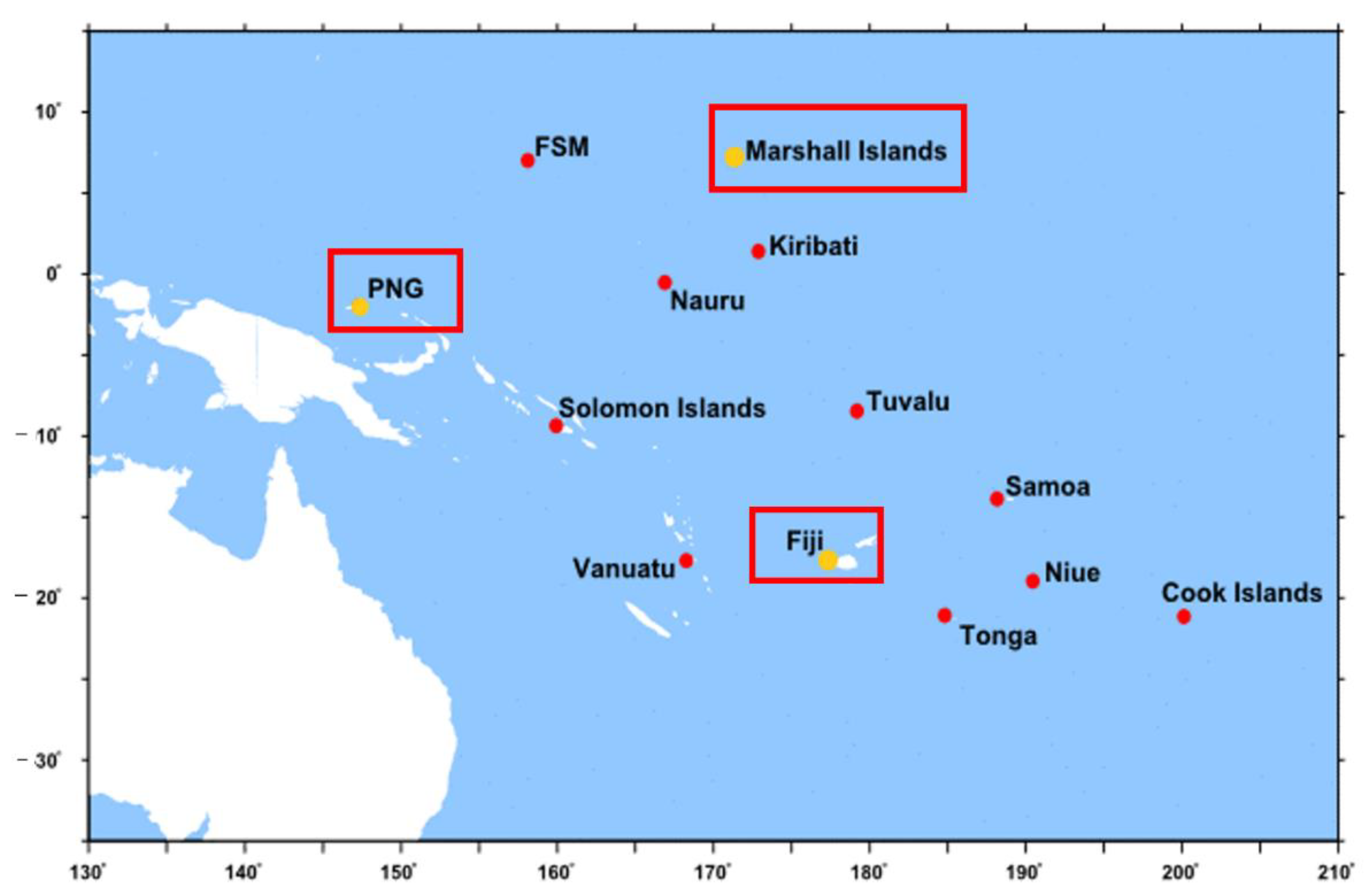
Figure 1. Study region showing the selected Pacific Islands (i.e., Fiji, Marshall Island and PNG). Source: Pacific Sea Level Monitoring Project (bom.gov.au, accessed on 10 May 2021).
Remotesensing 14 00986 g001
Figure 2. Time series of the intrinsic mode functions (IMFs) and the residual components after decomposing the MSL in the testing period using CEEMDAN. The time series of the actual MSL is plotted at the top of the figure.
Remotesensing 14 00986 g002
Figure 3. (a) Correlogram showing the covariance between the objective variable (MSL) and the predictor variables in terms of the cross-correlation coefficient (rcross) for Fiji stations and (b) Partial Auto Correlation Function (PACF) plot of the MSL time series exploring the antecedent behaviour in terms of the lag of MSL for every day (TWS—Terrestrial Water Storage, Tr—Transpiration, SurT—Average Surface Skin Temperature).
Remotesensing 14 00986 g003
Figure 4. An analysis of the statistically significant cross-correlation function plots of (a) IMF(s) and Residuals of Transpiration (Tr) vs. IMF(s) and Residuals of MSL accordingly, (b) Partial Auto Correlation Function (PACF) plot of the IMF(s) of MSL time series.
Remotesensing 14 00986 g004
Figure 5. Feature weight matrix of predictor variables using Neighbourhood Component Analysis (NCA) for MSL in the case of Fiji Islands.
Remotesensing 14 00986 g005
Figure 6. Topographical structure of the objective model used for forecasting MSL (a) 3-layered Convolutional Neural Network (CNN) and (b) 2-layered Gated Recurrent Unit Network (GRU).
Remotesensing 14 00986 g006
Figure 7. Methodological steps used in the model designing phase for the proposed hybrid CEEMDAN-CNN-GRU predictive models. Note: MSL = mean sea level, GRU = Gated Recurrent Unit, IMF = Intrinsic Model Function and NCA = Neighbourhood Component Analysis.
Remotesensing 14 00986 g007
Figure 8. The graphs show the mean sea level trend and computed rise per year for the period 1994–2020.
Remotesensing 14 00986 g008
Figure 9. Comparison of the forecasting ability of proposed models in terms of RRMSE (%) and WI in the testing phase.
Remotesensing 14 00986 g009
Figure 10. Box plots of hybrid models (CEEMDAN-CNN-GRU) along with their respective standalone counterparts (i.e., GRU, DT and SVR) in forecasted error (|FE|) in forecasting MSL of three selected Pacific Islands in the testing phase. The X symbol indicate the position of the mean in the box.
Remotesensing 14 00986 g010
Figure 11. Empirical Cumulative Distribution function (ECDF) of forecasted error |FE| of MSL generated by the proposed CEEMDAN-CNN-GRU along with comparing models for three selected sites in the testing phase.
Remotesensing 14 00986 g011
Figure 12. Scatter plot of forecasted vs. observed MSL of (a) Fiji Island, (b) Marshall Island, and (c) PNG using CEEMDAN-CNN-GRU and CNN-GRU model in the testing phase. A least square regression line and coefficient of determination (r2) with a linear fit equation are shown in each sub-panel.
Remotesensing 14 00986 g012
Figure 13. Bar graphs showing the Legate–McCabe’s Index (LM) with the proposed hybrid deep learning approach (CEEMDAN-CNN-GRU) in comparison with standalone models in the testing phase.
Remotesensing 14 00986 g013
Figure 14. Comparison between Forecasted and Observed MSL during the 2018–2020 period for the CEEMDAN-CNN-GRU model.
Remotesensing 14 00986 g014
Table 1. Description of the location of variables for MSL forecasting.
CountryPlaceLatitudeLongitude
FijiLautoka−2.0420147.3737
Marshall IslandsMajuro 7.1060171.3725
PNG Manus−17.6053177.4381
Table 2. Data partition breakdown with dates for the study sites.
PartitionTraining
(70%)
Validation
(15%)
Testing
(15%)
DatasetJanuary 1994–December 2012January 2013–December 2016January 2017–December 2020
Table 3. Results of the hybrid CEEMDAN-CNN-GRU vs. benchmark (CNN-GRU, CEEMDAN-GRU, GRU) models for three study sites. The correlation coefficient (r), root mean square error (RMSE; m), mean absolute error (MAE; m), relative mean absolute error (RMAE; %) and Nash–Sutcliffe coefficient, NS) are computed between forecasted and observed mean sea level (MSL) in the testing phase. The optimal model is boldfaced (blue).
ModelrNSRMSEMAERMAE
Station: Fiji
CEEMDAN-CNN-GRU0.9960.9930.0040.0030.239
CEEMDAN-GRU0.9590.9070.0140.0110.844
CEEMDAN-DT0.9270.8500.0180.0141.075
CEEMDAN-SVR0.8060.6050.0430.0352.767
CNN-GRU0.9820.9640.0090.0070.513
GRU0.9550.9090.0140.0110.841
DT0.8120.5640.0310.0241.819
SVR0.7930.5860.0440.0362.871
Station: Marshall Island
CEEMDAN-CNN-GRU0.9960.9910.0100.0060.628
CEEMDAN-GRU0.9790.9570.0110.0091.022
CEEMDAN-DT0.9620.9240.0190.0151.301
CEEMDAN-SVR0.8290.4920.0490.0383.289
CNN-GRU0.9890.9770.0110.0080.711
GRU0.9840.9670.0130.0100.851
DT0.9090.8100.0300.0242.133
SVR0.7660.4590.0510.0393.385
Station: PNG
CEEMDAN-CNN-GRU0.9950.9890.0070.0050.650
CEEMDAN-GRU0.9790.9570.0110.0091.022
CEEMDAN-DT0.8460.7080.0290.0222.705
CEEMDAN-SVR0.7210.4590.0550.0465.463
CNN-GRU0.9920.9840.0070.0050.637
GRU0.9790.9580.0110.0091.032
DT0.8460.7080.0290.0222.705
SVR0.7350.4510.0490.0404.759
Table 4. Legates and McCabe Index results of the hybrid CEEMDAN-CNN-GRU vs. benchmark (CNN-GRU, CEEMDAN-GRU, GRU) models for three study sites.
ModelsFijiMarshal IslandPNG
CEEMDAN-CNN-GRU0.91680.92710.9207
CEEMDAN-GRU0.70870.80340.8034
CEEMDAN-DT0.62890.73210.4824
CEEMDAN-SVR0.36260.31390.5702
CNN-GRU0.82130.85450.8778
GRU0.70850.82540.8026
DT0.3720.56310.4824
SVR0.33920.29430.3672
Publisher’s Note: MDPI stays neutral with regard to jurisdictional claims in published maps and institutional affiliations.