Article

An Analysis of Arctic Sea Ice Leads Retrieved from AMSR-E/AMSR2

1
College of Oceanic and Atmospheric Sciences, Ocean University of China, Qingdao 266100, China
2
Key Laboratory of Marine Hazards Forecasting, National Marine Environmental Forecasting Center, Ministry of Natural Resources, Beijing 100081, China
3
Department of Atmospheric and Environmental Sciences, University at Albany, State University of New York, Albany, NY 12222, USA
4
Key Laboratory of Polar Science of Ministry of Natural Resources, Polar Research Institute of China, Shanghai 200136, China
*
Author to whom correspondence should be addressed.
Remote Sens. 2022, 14(4), 969; https://doi.org/10.3390/rs14040969
Submission received: 22 December 2021 / Revised: 8 February 2022 / Accepted: 15 February 2022 / Published: 16 February 2022
(This article belongs to the Special Issue Remote Sensing Monitoring of Arctic Environments)

Abstract

:
In this study, we retrieve an Arctic sea ice lead fraction from AMSR2 passive microwave data in winter from 2012 to 2020 based on an algorithm developed for AMSR-E data. The derived AMSR2 sea ice lead fraction is validated against MODIS images. The results show that the derived AMSR2 sea ice lead detects approximately 50% of the ice leads shown in the MODIS images, which is close to the amount of sea ice lead detected from the AMSR-E data from 2002 to 2011. Utilizing the retrievals from both the AMSR-E and AMSR2, our analysis shows no significant trend, but moderate interannual variation exists for the ice lead fraction in the Arctic basin scale over the past two decades. The maximum width and total length of sea ice lead show a significant decreasing trend for the whole Arctic, but the mean width does not exhibit a significant change over the studied period. In the Beaufort Sea the lead fraction varies from 2.06% to 12.35%, with a mean value of 5.72%. In the Greenland Sea the mean lead fraction over the studied period is 5.77%, and there is a significant increase in the lead fraction, with a rate of 0.13% per year. The maximum width in the Greenland Sea is substantially higher than that of other regions, and the mean width increases significantly.

1. Introduction

Arctic sea ice has undergone an accelerated decline in recent decades. Sea ice extent has decreased at a rate of 3% per decade in the satellite era and up to 10% per decade in summertime sea ice extent [1,2]. Meanwhile, sea ice thickness has also reduced significantly [1,3], with a mean reduction of 2.34 m from 1975 to 2012 [4]. Future climate projections show that Arctic summertime sea ice extent may drop to ∼1.7 million km2 in the mid-2040s and that an ice-free Arctic may occur in the mid-2050s in the scenario of high emissions [5].
Sea ice leads, which are mainly caused by ice divergence or shear motion, are quasi-rectilinear openings in the pack ice zone. In the Arctic the length of sea ice leads varies from a few meters to hundreds of kilometers, and the width of sea ice leads ranges from several meters to several kilometers. Sea ice leads are more prevalent in the Arctic marginal seas than in the central Arctic [6,7,8,9]. In winter, sea ice leads play a very important role in the exchange of heat and moisture between the atmosphere and the ocean, and thus significantly affect the atmospheric state through turbulent heat release by the warm ocean. Studies have pointed out that sea ice leads accounted for more than half of turbulent heat exchange between the atmosphere and the ice zone, which directly changed the oceanic and atmospheric heat balance in the polar region [10,11,12,13,14,15,16,17].
Retrieving sea ice leads from observations provides a reference for sea ice dynamic research and sea ice modeling validation. Many methods have been proposed to detect sea ice leads with different data from different platforms; for example, early observations based on aircraft have long been collected to study the surface energy balance and formation of sea ice leads in the Arctic [18,19,20], but these aircraft-based observations are far from enough. Along with the development of remote sensing technology based on polar-orbiting satellites, attention has been paid to identifying sea ice leads from satellite data [21,22,23,24,25,26,27,28,29,30,31,32,33,34]. Miles and Barry [9] generated a five-year climatological dataset of sea ice leads in the Arctic Ocean using Defense Meteorological Satellite Program optical imagery. Their work provided a first impression of Arctic sea ice leads in the early 1980s; however, retrieving sea ice leads from optical imagery was easily affected by dark seasons and cloudy conditions. Lindsay and Rothrock [6] developed an automatic detection algorithm of sea ice leads based on advanced very-high-resolution radiometer (AVHRR) images. Röhrs and Kaleschke [24] presented an algorithm to detect sea ice leads in the Arctic Ocean based on Advanced Microwave Scanning Radiometer for the Earth Observing System (AMSR-E) microwave imagery. The algorithm was based on the unique signatures of thin ice in the brightness temperature ratio between the 89.0 GHz and 18.7 GHz channels. Following the algorithm, a nine-year climatology of lead orientation and lead frequency in Arctic sea ice was generated from the AMSR-E data [25]. Many studies focused on the detection of sea ice leads from Moderate Resolution Imaging Spectroradiometer (MODIS) data, despite potential cloud contamination. Willmes and Heinemann [26,27,28] presented a sea ice lead detection method utilizing the MODIS ice surface temperature product and generated a dataset of sea ice leads in the Arctic from 2003 to 2015. However, cloud artifacts were present in the lead identification, which were caused by ambiguities in the MODIS cloud mask. Reiser et al. [29] introduced a daily sea ice lead dataset at a resolution of 1 km2 for the winter months—November–April 2002/03–2018/19 (Arctic) and April–September 2003–2019 (Antarctic)—based on MODIS thermal infrared images. Hoffman et al. [30,31] proposed an algorithm that detected sea ice leads from MODIS data using brightness temperature at the ~11 µm waveband with an observational angle of less than 30° and published a climatological dataset of Arctic sea ice leads. Qu et al. [33] proposed a method with multiple thresholds to retrieve the spring sea ice lead distribution in the Beaufort Sea using Terra/MODIS level-1B images and adapted a daily-averaged scheme to minimize the influence of ice motion. Moreover, a new approach that utilized artificial intelligence was also proposed to detect sea ice leads from MODIS thermal infrared images [34]. Furthermore, sea ice leads can be retrieved from synthetic aperture radar (SAR) images as well as satellite altimetry [35,36,37,38,39].
Characterizing the long-term evolution of sea ice leads in the Arctic Ocean provides benefits for the polar climate research community. The family of AMSR sensors provides a suitable platform for long-term sea ice lead identification. The AMSR2 sensor onboard the Global Change Observation Mission 1st-Water (GCOM-W1) satellite was launched in 2012. Since there is no existing open access sea ice lead product based on AMSR2 data, in this study we derive sea ice leads in the Arctic from AMSR2 brightness temperature data based on the algorithm introduced by Röhrs and Kaleschke [24] and analyze the long-term variations in Arctic sea ice leads from 2002 to 2020 utilizing both AMSR-E and AMSR2 data. The rest of this paper is organized as follows: Section 2 briefly introduces the data sources and Section 3 presents the retrieving algorithm for sea ice lead fractions and lead geometry. Section 4 illustrates the validation of derived sea ice lead fractions against MODIS images and analyzes the long-term variations in sea ice lead orientation, length, and width in different Arctic regions during 2002–2020. A discussion is presented in Section 5. Our conclusion is presented in Section 6.

2. Data

2.1. AMSR2 Data

As the successor of the AMSR-E sensor onboard the NASA Aqua satellite, the AMSR2 sensor onboard the JAXA GCOM-W1 satellite was launched in May 2012 and has been delivering data since August 2012. AMSR2 is a multi-frequency microwave radiometer which measures microwave emissions at frequencies between 6.9 GHz and 89.0 GHz from the earth’s surface and the atmosphere. AMSR2 provides highly accurate measurements of microwave emissions and scattering at a height of approximately 700 km above the earth’s surface. The antenna of AMSR2 rotates once per 1.5 seconds and obtains data over a 1450 km swath. thus it has the capacity to acquire a set of daytime and nighttime data every two days with an earth surface coverage of more than 99%. The AMSR2 L1B global swath brightness temperature is available from JAXA (https://gportal.jaxa.jp/gpr/) (accessed on 3 June 2020). The swath data, including ascending and descending orbits, are archived in an HDF5 format. Vertically polarized brightness temperatures at 18.7 GHz and 89.0 GHz are used in this study to retrieve AMSR2 sea ice leads. AMSR2 brightness temperature data cover cold seasons from 2012 to 2020; here, the cold seasons refer to months from November to April of the next year. The AMSR-E sea ice leads in cold seasons from 2002 to 2011 used in Section 4 are accessed from the University of Hamburg (obtained at https://www.cen.uni-hamburg.de/en/icdc/data/cryosphere/lead-area-fraction-amsre.html) (accessed on 3 June 2020).

2.2. MODIS Datasets

We chose three sea ice lead products derived from the MODIS data as references with which to validate the AMSR2 sea ice leads. (1) Willmes and Heinemann [26,27,28] applied a binary segmentation procedure to MODIS thermal imagery to identify sea ice leads on a daily basis and mapped pan-Arctic sea ice lead distributions from January–April in the period of 2003–2015. The derived sea ice leads in the dataset are separated into two uncertainty categories, with high uncertainty being attributed to artifacts that arise from warm signatures of unrecognized clouds. The dataset, denoted by WHD hereafter, is obtained at https://doi.pangaea.de/10.1594/PANGAEA.854411 (accessed on 15 August 2020) with a spatial resolution of less than 2 km2. (2) Hoffman et al. [30,31] developed an algorithm to detect and characterize sea ice leads using a satellite thermal infrared window channel and published an Arctic sea ice lead dataset at a daily resolution since 2002 (obtained at ftp://frostbite.ssec.wisc.edu, accessed on 15 August 2020 and denoted by HD hereafter). The derived sea ice leads are provided at a 1 km spatial resolution and classified into several categories, including positively identified leads and some rejection categories. A cloud mask, a coverage array that reports the number of cloud-free overpasses, and a potential lead array are included in the daily data files. (3) Qu et al. [33] presented a modified algorithm using multiple thresholds and daily scores to retrieve spring sea ice leads in the Beaufort Sea. Their method was based on a temperature anomaly obtained from Terra MODIS thermal images. The spatial resolution of the product is also 1 km, and the product provides a daily sea ice lead fraction in the Beaufort Sea in April from 2001 to 2020 (denoted by QD hereafter).

3. Method

3.1. Retrieve Sea Ice Leads from the AMSR2 Brightness Temperature

Röhrs and Kaleschke found that thin ice has a unique signature in the emissivity radio in the vertically polarized brightness temperature channels at frequencies between 89.0 GHz and 18.7 GHz in winter [24]. The different sea ice classes, especially for water and thin ice, are characterized by emissivity ratios above one. Additionally, a mean filter is used to enhance the signal of the leads. The proposed algorithm exhibits advanced ability in detecting sea ice leads in the pack ice zone. It detects sea ice leads wider than 3 km and resolves about 50% of the lead area compared to MODIS satellite images. Following the proposed algorithm, we derive sea ice lead fractions from AMSR2 brightness temperature data. The following procedures are carried out:
(1)
Interpolate the AMSR2 L1B brightness temperatures at frequencies of 18.7 GHz (TB,18.7V) and 89.0 GHz (TB,89V) onto the National Snow and Ice Data Center (NSIDC) EASE grid with a spatial resolution of 6.25 km. For 89.0 GHz data, a bilinear interpolation scheme is used. For 18.7 GHz data, a nearest-neighbor interpolation scheme is used;
(2)
Calculate the brightness temperature ratio (r) following Equation (1):
r = T B , 89 V T B , 18 . 7 V
(3)
Calculate the brightness temperature ratio anomalies ( r ) according to Equation (2):
r = r M e d i a n w ( r )
where Medianw(r) represents the utilization of a median filter to r in all grid points surrounding the target grid point with a w × w search window. The large AMSR2 sensor’s footprint means that a potential lead signal might be a mixture of narrow lead and thick ice; thus, sea ice leads in the pack ice zone are more representative by r than by r;
(4)
Calculate the lead fraction (LF) following Equation (3). The lead fraction is defined as the area fraction of thin ice compared to the area fraction of other ice classes.
LF = { 1 if   r > r 100 0 if   r < r 0 r r 0 r 100 r 0 if   else
where r 100 denotes the upper tie point and r 0 denotes the lower tie point. Following Röhrs and Kaleschke [24], w, r 100 , and r 0 are set to 7, 0.05, and 0.015, respectively.
After the implementation of the abovementioned steps, some postprocess procedures are applied to the lead fraction field to reduce the unrealistic signal. Isolated lead pixels are removed to reduce the number of fragments, and a near-coastal grid cell, which is one or two grid cells away from the coast, is also removed due to potential land spill/contamination [38], although these grid cells normally have large lead fraction values. Figure 1 shows the spatial patterns of vertically polarized brightness temperatures at the frequencies of 89.0 GHz and 18.7 GHz, the brightness temperature radio and its anomaly, as well as the lead fraction on 23 February 2013. The brightness temperature at the frequency of 89.0 GHz is characterized by a high value over open ocean and a low value over ice packs; the brightness temperature in the pack ice zone north of the Canadian Arctic Archipelago is lower than that in the marginal ice zone on the Eurasian continent side (Figure 1a). The vertically polarized brightness temperature at the frequency of 18.7 GHz is characterized by a high value over ice packs and a low value over open ocean (Figure 1b). The brightness temperature radio between the frequencies of 89.0 GHz and 18.7 GHz shows a relatively smooth pattern with visible large linear shapes in the Beaufort Sea (Figure 1c). The pattern of the brightness temperature radio anomalies clearly presents linear shapes with different sizes, and sea ice leads in the pack ice zone are highly visible in the pattern (Figure 1d). The map of the lead fraction (Figure 1e) generally follows the pattern of the brightness temperature radio anomalies.

3.2. Statistics of Lead Geometry

Sea ice lead geometry on statistics is a mirror of mean-state evolution in sea ice thickness, sea ice age, and sea ice stress driven by oceanic and atmospheric forcing. Lindsay and Rothrock [6] found that the lead width distribution derived from AVHRR imagery follows a power law formula, in which the exponent varies with the change of seasons. Studies have pointed out that the exponent in the power law formula increased along with the finer spatial resolution of target datasets [13,32]. Many approaches were proposed to measure the orientation and length of sea ice leads in previous studies, such as the local gradient in an image (Sobel operator), 2D-Fourier transform, skeleton orientations and direction of maximum extent [6], as well as Hough transform [25,31,40].
We use the algorithm introduced in Qu et al. [33] to identify sea ice lead orientation, width, and length. The algorithm can quickly solve sea ice lead geometry by applying a directional lead extent operator to a sea ice lead field. Basically, the lead orientation is defined as the angle of rotating the 45°W longitudinal line anticlockwise to parallel to the main direction of the target lead. The overall length, Li, for lead width, Xi, can be calculated as follows:
L i = a 0 2 N i X i = a 0 N i i
where a0 is the pixel resolution and Ni is the number of pixels for width X i = a 0 i (I = 1, 2, 3…). The mean width, xm, can be derived from the regional lead area, S, divided by the total length of leads:
x m = S L = S L i
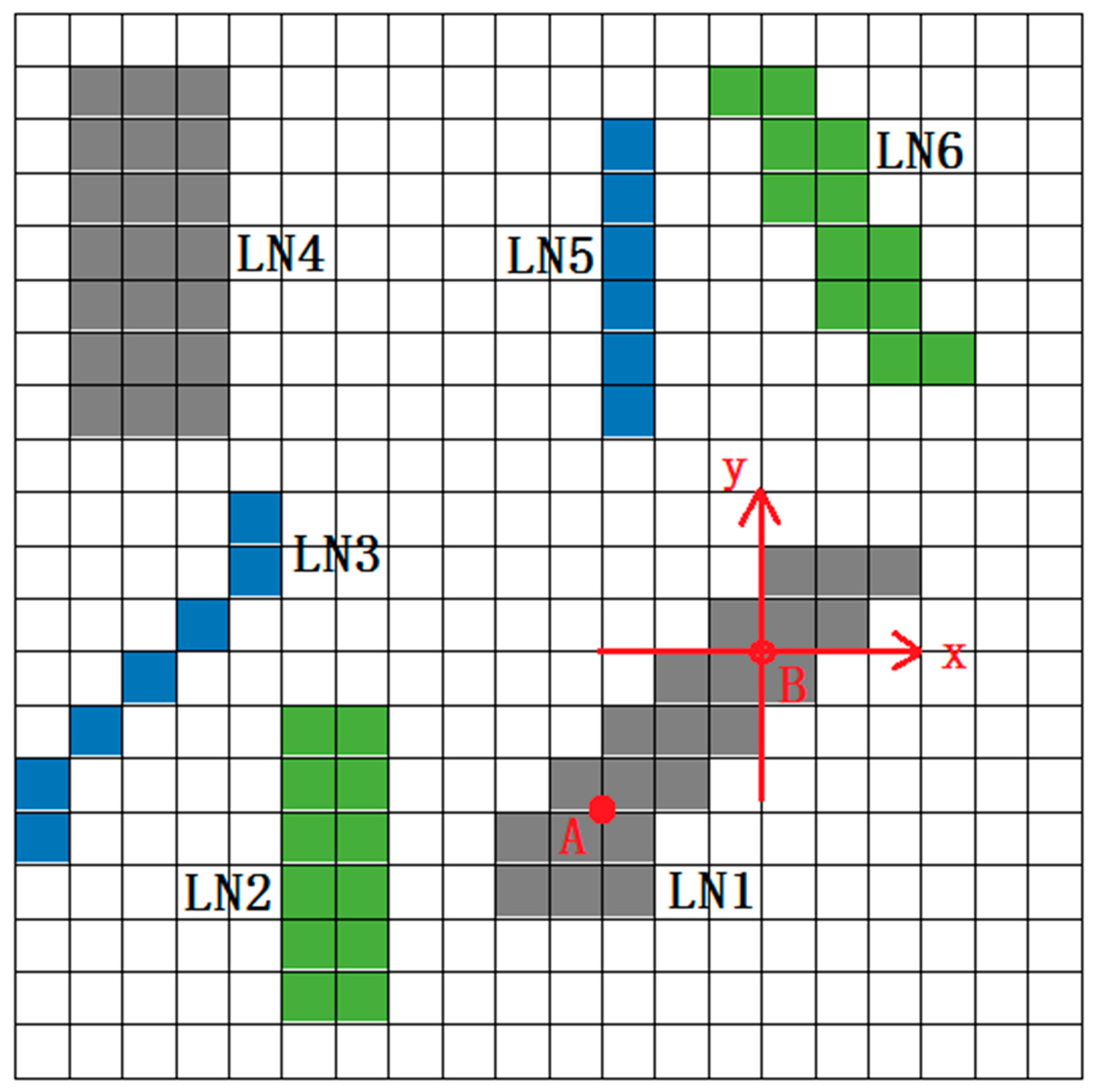
Figure 2 shows a schematic of sea ice geometry. Assume that there are six different sea ice leads in the study domain with an area of 20 × 20 pixels. In the AMSR2 sea ice lead products the resolution of the pixel is 6.25 km. To calculate Li we need to calculate the lead width for each sea ice lead at first. Taking lead number 1 (LN1) as an example, (1) we define orthogonal coordinates (x, y) with the original point located at the left–down corner of one pixel. Note that this pixel should be in LN1. Then, we acquire the short span in x and y directions. In the case of the original point being located at point B, the span in x direction is 3 pixels, the span in y direction is 3 pixels, then the short span is 3 pixels. In the case of the original point being located at point A, the span in x direction is 3 pixels, the span in y direction is 4 pixels, then the short span is 3 pixels. (2) The orthogonal coordinates are iterated with the original point located at the left–down corner of each pixel in LN1, and the lead width of LN1 is the shortest span in all iterations except the iterations at two ends of the length direction of the lead. The lead width of LN1 spans 3 pixels, i.e., 18.75 km.
After acquiring the lead width of all six sea ice leads, we can classify sea ice leads in the study area into several types by lead width. In Figure 2 there are three types: gray leads (LN1 and LN4), with a lead width spanning 3 pixels, green leads (LN2 and LN6), with a lead width spanning 2 pixels, and blue leads (LN3 and LN5), with a lead width spanning 1 pixel. Then, following Equation (4), the overall length, Li, for lead width, Xi, can be calculated as:
L 1 = 6.25 × 6.25 × 13 6.25 × 1 = 81.25   km
L 2 = 6.25 × 6.25 × 24 6.25 × 2 = 75   km
L 3 = 6.25 × 6.25 × 42 6.25 × 3 = 87.5   km
where 13, 24, and 42 are the numbers of blue, green, and gray pixels. Following Equation (5), the mean width, xm, can be derived by:
x m = 6.25 × 6.25 × 79 81.25 + 75 + 87.5 = 12.66   km
where 79 is number of all color pixels in the study domain. It is noteworthy that using orthogonal coordinates to identify the lead width tends to overestimate the lead width due to a mismatch between the preset direction and the orientation of the lead; but the orthogonal system will help contain the error. The derived lead width will be smaller than 2 times the real lead width [32].

4. Results

4.1. Validation of the Derived Sea Ice Leads on 3 April 2013

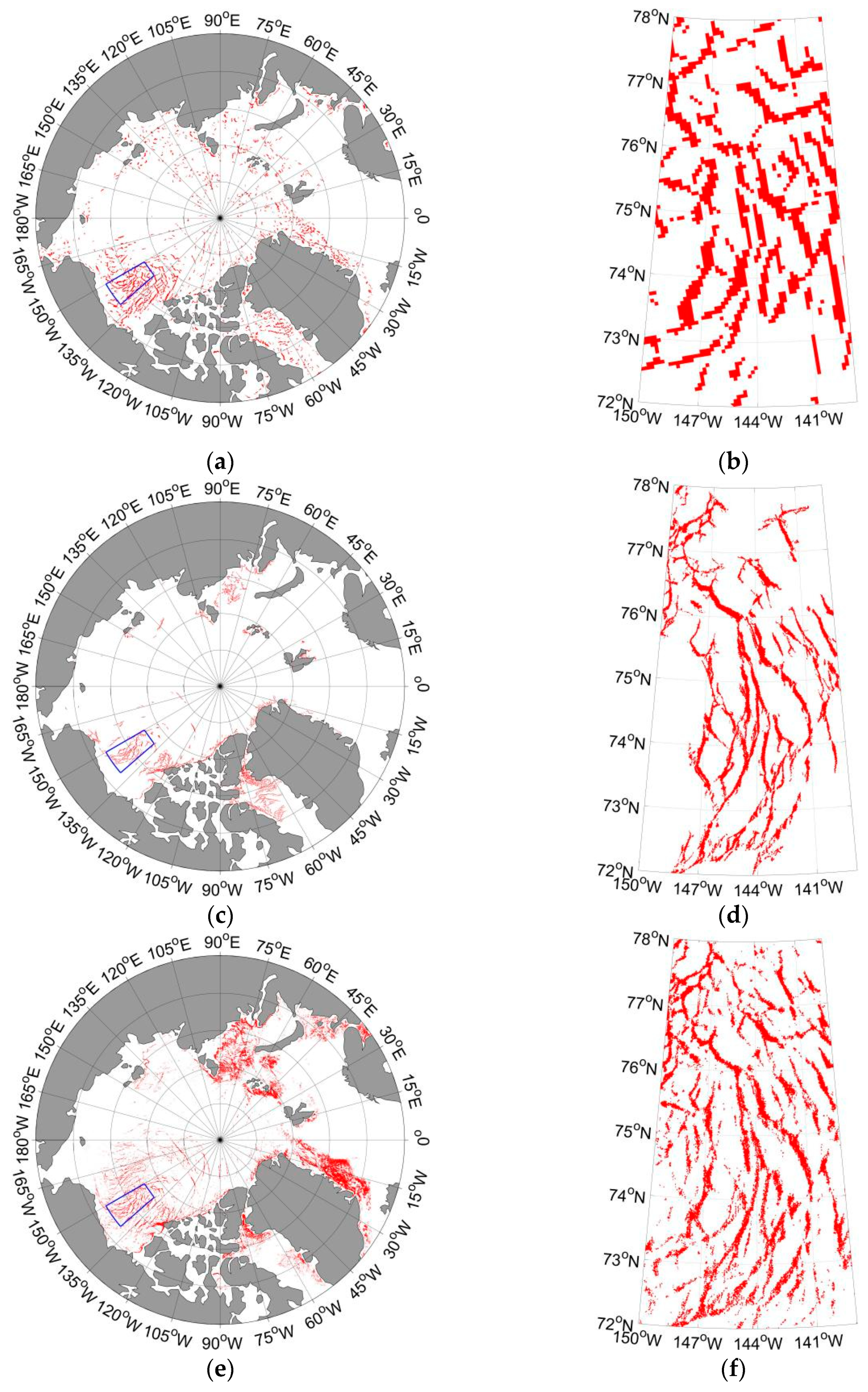
In this section we compare the detected sea ice leads from the AMSR2 data on 3 April 2013 with the three sea ice lead products from the MODIS data (Figure 3). Specifically, we zoom in on the Beaufort Sea to illustrate the details of the derived sea ice leads because that sea ice exhibits strong rheological features in the Beaufort Sea, such as sea ice ridges and leads. The detected sea ice leads with a lead fraction less than 1% in the AMSR2 data are negligible since these leads may come from noise on the daily map. Only completely identified sea ice leads from the MODIS dataset are taken into calculation; potential sea ice leads are excluded.
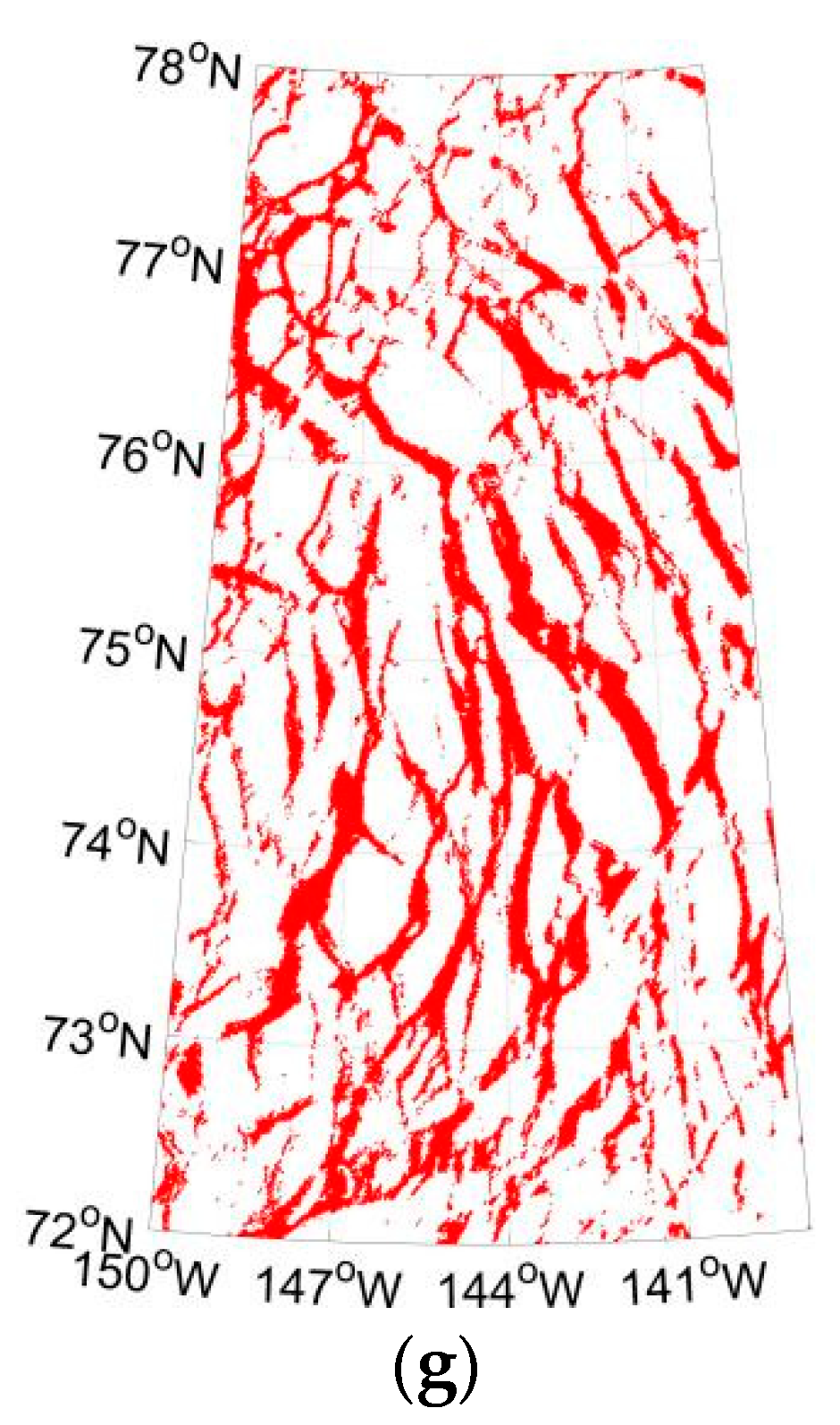
Basically, the derived sea ice leads in the AMSR2 data (Figure 3a) show similar patterns to those in the HD (Figure 3c) and WHD (Figure 3e) products, that is, sea ice leads are prevalent in the Beaufort Sea, Kara Sea, Greenland Sea, and Baffin Bay. The WHD product presents more sea ice leads than the HD product in the Beaufort Sea, Kara Sea, and Greenland Sea. In the Beaufort Sea, the derived sea ice leads in the AMSR2 data (Figure 3b) generally represent typical sea ice geometry, which is identified in the three MODIS datasets (Figure 3d–g). Owing to the relatively coarser resolution in the AMSR2 data, the three MODIS sea ice lead products exhibit finer regional variations. To further quantitatively validate our results these MODIS products have been resampled and remapped with a nearest-neighbor technique to match our product. Statistical comparison shows that the derived AMSR2 sea ice leads in the Beaufort Sea on 3 April 2013 capture 46.91%, 47.53%, and 40.06% of the leads shown in the HD, WHD, and QD products. Since the cloud masks in the three MODIS data are different, these values are acquired after the removal of the AMSR2 grid points, which are covered by cloud in the corresponding MODIS product. These values are comparable with the value of 50% of lead detection for AMSR-E data [24].

4.2. Long-Term Evolution of Lead Fraction and Geometry in the AMSR Family Data

Since the algorithm used in retrieving sea ice leads from the AMSR2 data is consistent with that in the AMSR-E sea ice lead product, we analyze long-term variations in the Arctic sea ice leads utilizing observations during the lifespan of both the AMSR-E and AMSR2 sensors; that is, from November 2002 to April 2020, except for the period with a data gap between November 2011 and April 2012.
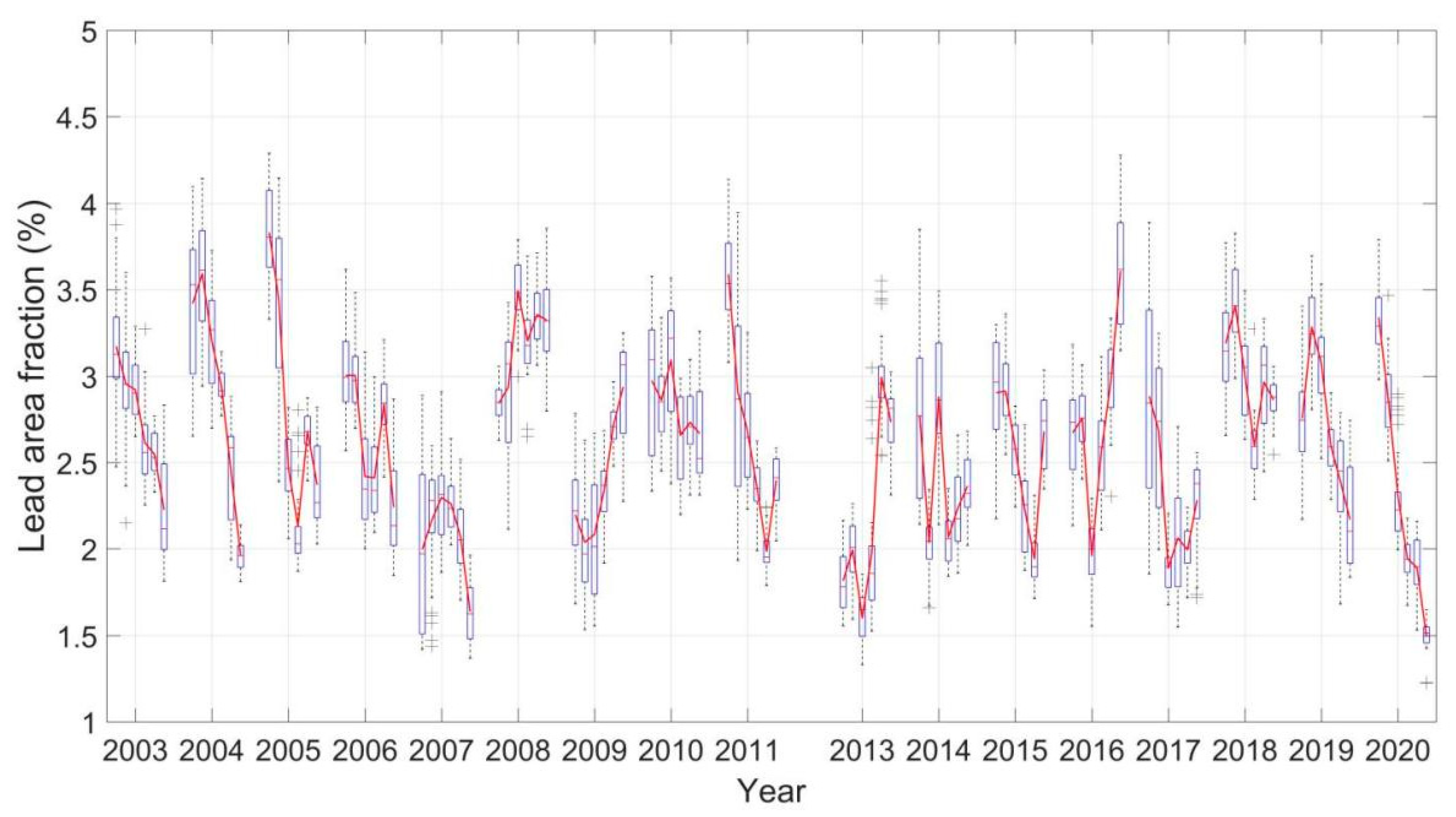
The monthly evolution of the lead fraction in the cold seasons in the Arctic north of 65°N is shown in Figure 4. In general, there is no significant change in the lead fraction between the AMSR-E and AMSR2 periods. Wang et al. [41] found similar results in model simulation during 1985–2014, and they attributed the reason to the absence of a significant trend in the surface wind stress in the Arctic atmosphere. The climatological lead fractions from November to April during the whole observation timespan are 2.87%, 2.79%, 2.56%, 2.39%, 2.49%, and 2.45%, respectively. It is noteworthy that the lead fraction shows moderate interannual variation in the whole Arctic, ranging from 2.06% in 2006/2007 to 3.18% in 2007/2008.
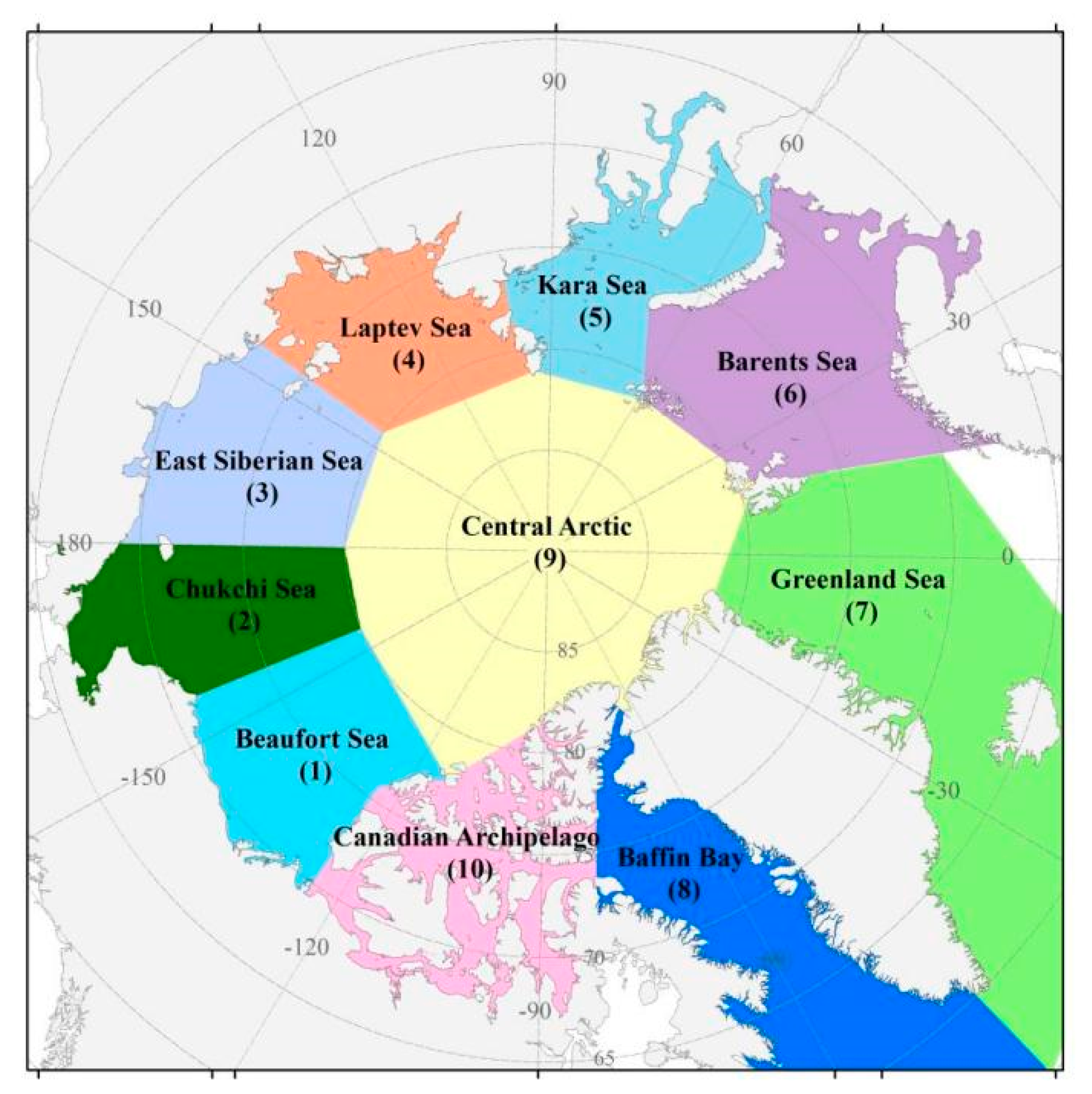
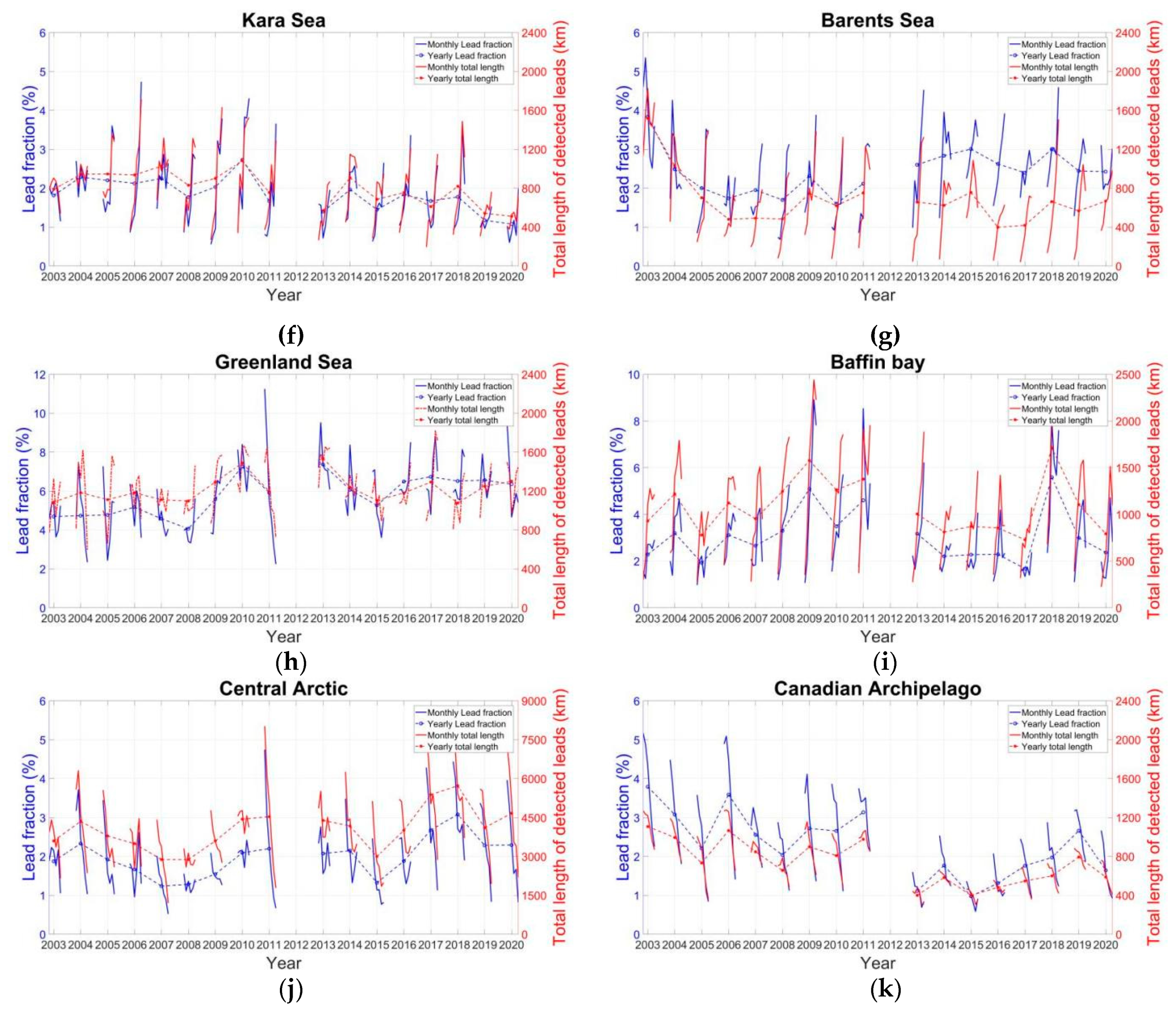
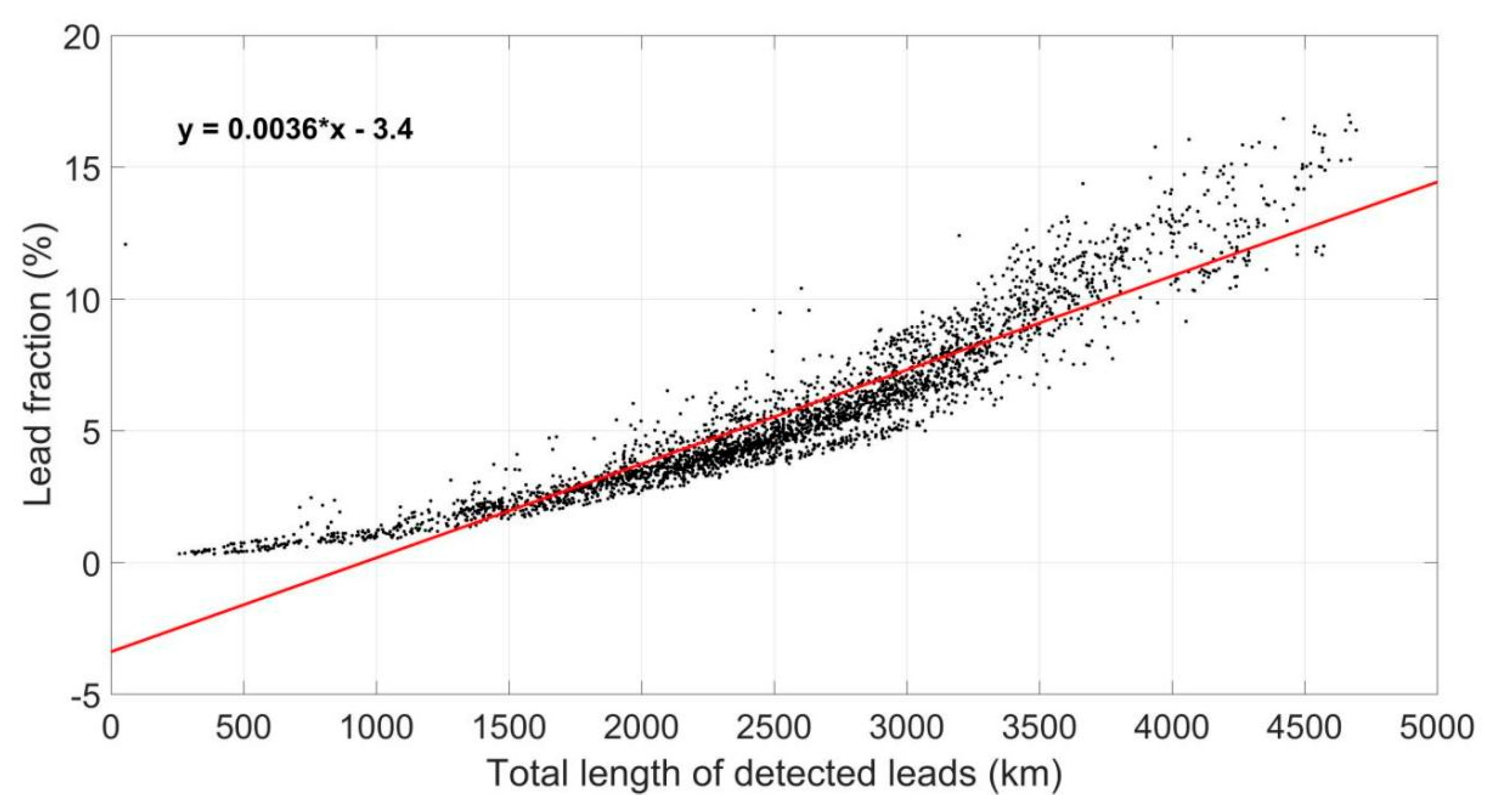
We further divide the Arctic Basin into 10 regions to study the regional differences in the lead fraction (Figure 5). The division of the study areas follows Fetterer et al. [42]. Figure 6 shows the evolution of the sea ice lead fraction and the total length of sea ice leads in different regions in the AMSR family data. The annual values of the sea ice lead fraction retrieved from the AMSR family data are listed in Table 1. In the central Arctic, the annual lead fractions vary from 1.24% to 3.08% during the whole observation timespan, and there is a significant increase in the sea ice lead fraction in the years after 2016 compared to before 2007, indicating that features in sea ice dynamics may have changed substantially in the central Arctic. Compared with other regions, the annual lead fraction shows larger values in the Beaufort Sea and Greenland Sea. In the Beaufort Sea the sea ice lead fraction varies from 2.06% in 2016/2017 to 12.35% in 2007/2008, with a mean value of 5.72%. In the Greenland Sea there is an obvious increase in the sea ice lead fraction, with a rate of 0.13% per year at a 95% significance level; the lead fractions remain stably between 4.06% and 7.37%; and the mean lead fraction over the studying period is 5.77%. It is noteworthy that the sea ice leads in the Baffin Bay increase sharply in 2008/2009, 2010/2011, and 2017/2018. Furthermore, there is a decrease in the sea ice lead fraction in the Eastern Siberia–Laptev–Kara Sea from the AMSR-E period to the AMSR2 period, probably relating to the changes in wintertime sea ice properties in the past two decades. Partly owing to the relative coarser spatial resolution, the annual sea ice lead fractions derived from the AMSR2 data are comparable to the results in Hoffman et al. [31] but smaller than those in Willmes and Heinemann [26]. The total length of sea ice leads is highly correlated to the sea ice lead fraction in all regions (Figure 7). The correlation coefficient is as high as 94% in daily maps.
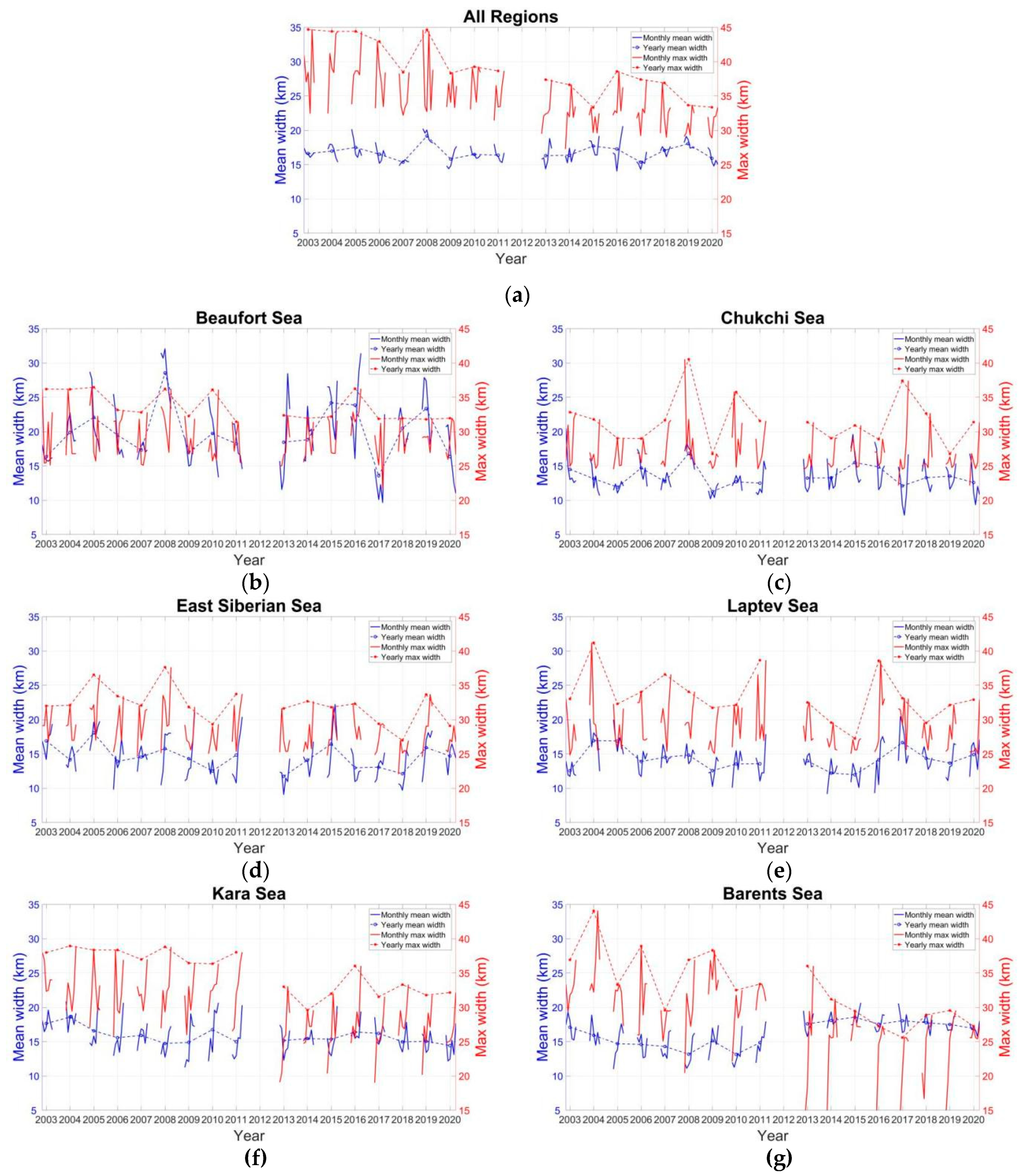
Figure 8 shows the evolution of the maximum width and mean width of Arctic sea ice leads in different regions in the AMSR family data. Both the maximum width and total length of the sea ice leads show a clearly decreasing trend in the whole Arctic by 0.62 ± 0.08 km/year and 130 ± 50 km/year, respectively. However, mean width does not exhibit a significant change over the studied period. The maximum width of sea ice leads in the Greenland Sea, which ranges from 31.9 km to 44.7 km, is substantially higher than that of other regions. The mean width of sea ice leads in the Greenland Sea increases significantly by 0.16 ± 0.04 km per year at a 95% confidence level. The total length of sea ice leads in the Greenland Sea does not show any significant trend. In the Beaufort Sea the mean width and total length of sea ice leads do not evidently change, but a slightly decreasing trend in the maximum width is identified. Note that the mean width of sea ice leads in the Greenland Sea and Beaufort Sea is usually larger than that of other seas. Main lead orientations lie in 0°–10°, 40°–50°, 90°–100°, and 130°–140° in most seas (not shown).
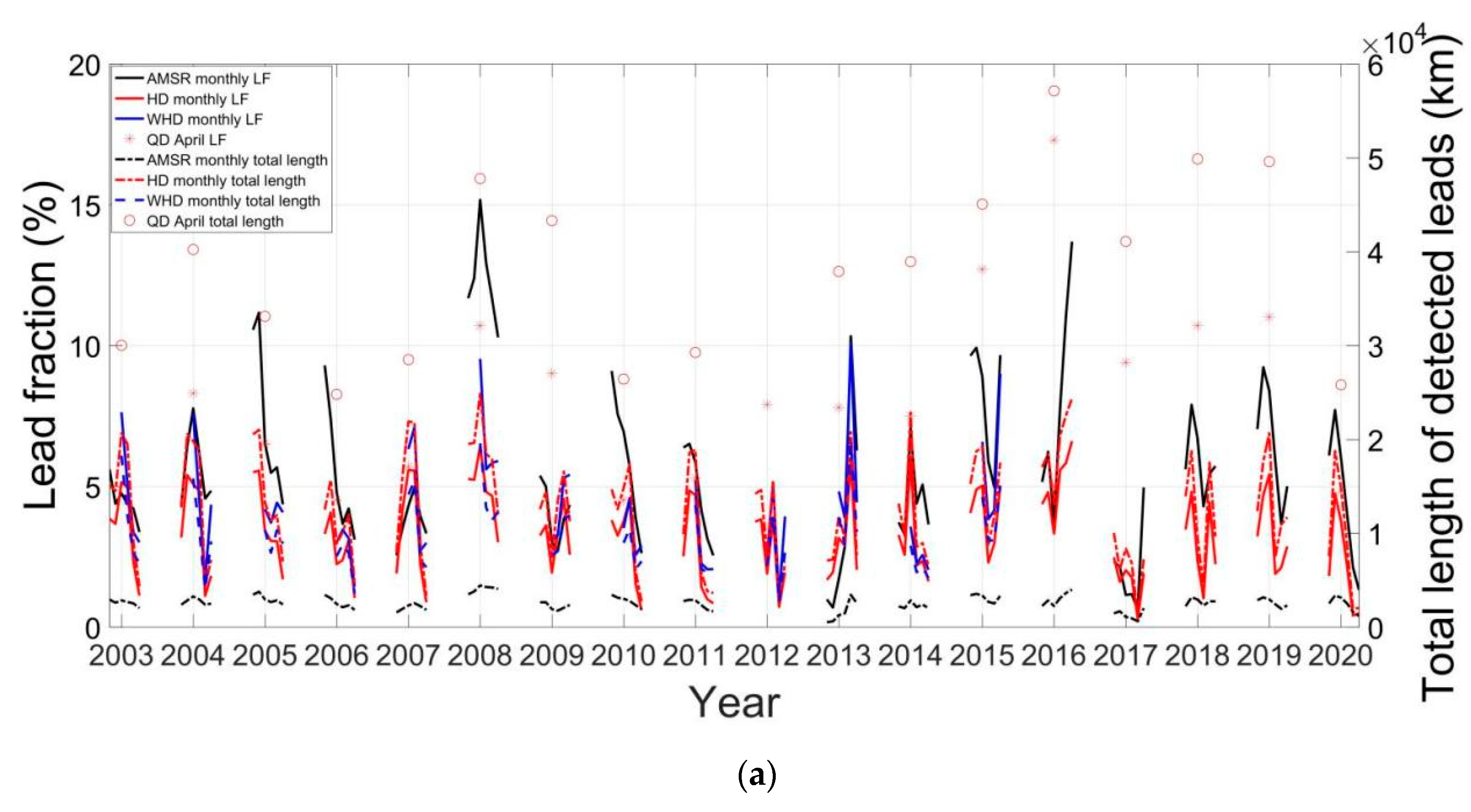
Finally, we compare our results in the Beaufort Sea with those values identified from the three MODIS datasets. The Beaufort Sea is selected because sea ice leads are prevalent in this region and the QD product only covers this region. The comparison shows that the sea ice lead fraction in the AMSR family data is generally larger than that of the WHD and HD products, but smaller than the QD product in years after 2010. However, the total length of sea ice leads (1.17 × 10³ km to 4.07 × 10³ km) in the AMSR family data is much smaller than the three MODIS data (Figure 9a). This result probably comes from the fact that sea ice leads with a width less than 6.25 km cannot be retrieved from the AMSR family data. The maximum width (25.4 km to 36.3 km) in the AMSR family data is generally smaller than the WHD product but larger than the HD and QD products. The mean width (11.0 km to 31.4 km) in the AMSR family data is larger than the three MODIS datasets, probably owing to the relatively coarse resolution.

5. Discussion

Detecting sea ice leads from microwave passive data can avoid or be less affected by the influence of cloud, but they nevertheless have a coarse resolution. Although the thermal infrared images have a finer resolution, retrieving sea ice leads from thermal infrared data is heavily affected by cloud. In this study we present a preliminary analysis of the long-term evolution of sea ice leads in the Arctic derived from the AMSR family microwave data. The presented result is basically reliable under several preconditions: (1) The threshold values r 100 and r 0 used in Equation (3) in deriving the sea ice lead fraction from the AMSR2 data are consistent with those used in AMSR-E data [24]. (2) The derived sea ice leads from the AMSR family data are less affected by weather conditions, although the brightness temperature at the frequency of 89.0 GHz still suffers from some weather conditions. (3) The analysis of the long-term evolution is conducted on the basis of annual mean values, which reduce the uncertainty of daily maps owing to data quality problems on a single date.
The sea ice leads are determined by the anomaly in brightness temperature ratio between the frequencies of 89.0 GHz and 18.7 GHz. Since the footprint of the brightness temperature at the frequency of 89.0 GHz is 3 × 5 km, while that of 18.7 GHz is 14 × 22 km, different interpolation schemes are used in interpolating the original data onto the EASE grids with a resolution of 6.25 km. For the 89.0 GHz data a bilinear interpolation scheme is used. For the 18.7 GHz data a nearest-neighbor interpolation scheme is used. The selection of the different interpolation schemes potentially reduces the uncertainty in the derived AMSR2 sea ice leads, which may be induced by a difference in the resolutions of the original data. Besides, the scans at the frequency of 89.0 GHz have two channels: 89.0A and 89.0B. We compared the derived sea ice leads on 3 April 2013 utilizing 89.0A, 89.0B, and 89.0(A + B), and found that the identification rate of utilizing 89.0(A + B) is close to that of utilizing 89.0A or 89.0B. It is noteworthy that the time spent generating a sea ice lead field from the 89.0B data is shorter than that from the 89.0A or 89.0(A + B) data. From the consideration of computation efficiency, we decided to use 89.0B data in our final procedure.
On the other hand, since the resolution of the AMSE family data used in this work is 6.25 km, the sea ice lead width and length identified in the AMSR family data are multiples of 6.25 km; thus, our analyses are restricted to the Arctic sea ice leads with a relatively large size. Fine leads with a width less than 5 km are not resolved in the AMSR sea ice lead product. Our result shows that the mean width of sea ice leads in the Arctic does not exhibit a significant change over the past two decades. This result may not be solid because the change in the mean width may be too small for the instrument to resolve.

6. Conclusions

In this study we retrieved Arctic sea ice leads from the AMSR2 brightness temperature data following the algorithm proposed by Röhrs and Kaleschke [24] and briefly analyzed the long-term evolution of the Arctic sea ice leads utilizing data from the AMSR family. The comparison between the derived AMSR2 sea ice leads and MODIS products shows similarity in most prominent lead structures throughout the entire Arctic, with small differences at a regional scale owing to the different spatial resolutions.
Over the past two decades there is no significant trend in the sea ice lead fraction in the Arctic, but moderate interannual variation exists in the sea ice lead fraction on the Arctic Basin scale. Variations in the wintertime sea ice lead fraction can be largely explained by sea ice divergence variations, which are driven by surface winds associated with variations in atmospheric circulation. The interannual variations in wintertime atmospheric circulation may play an important role in driving the interannual variations in the sea ice lead fraction. The total length of sea ice leads is highly correlated to the sea ice lead fraction. Both the maximum width and total length of the sea ice leads show a clearly decreasing trend in the whole Arctic by 0.62 ± 0.08 km/year and 130 ± 50 km/year, respectively. However, the mean width does not exhibit a significant change over the whole interested period. At a regional scale, the annual lead fractions in the central Arctic vary from 1.24% to 3.08% during the whole observation timespan. In the Beaufort Sea the sea ice lead fraction varies from 2.06% in 2016/2017 to 12.35% in 2007/2008, with a mean value of 5.72% during the studied period. In the Greenland Sea there is an obvious increase in the sea ice lead fraction with a rate of 0.13% per year, and the lead fractions remain stably between 4.06% and 7.37%. The maximum width ranges from 31.9 km to 44.7 km, which is substantially higher than that of other regions. The mean width increases significantly by 0.16 ± 0.04 km per year during the whole observation timespan.
The detection of sea ice leads from passive microwave data is affected by the ice surface condition. Sea ice geometry is also affected by several thresholds in resolving sea ice lead width and orientation. In conclusion, the analysis of long-term variance in the Arctic sea ice leads in this study is quite preliminary. Moreover, apart from the mentioned variables in describing sea ice leads, other variables, such as lead area, are also useful to the characterization of sea ice leads. In the future a detailed study on the Arctic sea ice leads relating to Arctic climate change and sea ice dynamics could be conducted via a combination of numerical modeling and observational statistics.

Author Contributions

M.L. wrote the manuscript; M.L. processed and analyzed the data; J.L., X.L., M.Q. and Z.Z. designed the study and analyzed the results. All authors provided substantial input to the interpretation of the results. All authors have read and agreed to the published version of the manuscript.

Funding

This research was funded by the National Key R&D Program of China (2018YFC1407200, 2019YFE0105700 and 2018YFA0605901).

Data Availability Statement

All analyses in the study will be freely available to the public. Data requests can be sent to M.L. ([email protected]).

Acknowledgments

We thank the JAXA for providing the brightness temperature data, and the University of Hamburg for providing the AMSR-E lead fraction for the Arctic.

Conflicts of Interest

The authors declare no conflict of interest.

References

  1. Parkinson, C.L.; Cavalieri, D.J.; Gloersen, P.; Zwally, H.J.; Comiso, J.C. Arctic Sea ice extents, areas, and trends, 1978–1996. J. Geophys. Res. Earth Surf. 1999, 104, 20837–20856. [Google Scholar] [CrossRef]
  2. Comiso, J.C.; Parkinson, C.L.; Gersten, R.; Stock, L. Accelerated decline in the Arctic Sea ice cover. Geophys. Res. Lett. 2008, 35, L01703. [Google Scholar] [CrossRef] [Green Version]
  3. Kwok, R.; Sulsky, D. Arctic Ocean Sea ice thickness and kinematics: Satellite retrievals and modeling. Oceanography 2010, 23, 134–143. [Google Scholar] [CrossRef]
  4. Lindsay, R.; Schweiger, A. Arctic Sea ice thickness loss determined using subsurface, aircraft, and satellite observations. Cryosphere 2015, 9, 269–283. [Google Scholar] [CrossRef] [Green Version]
  5. Liu, J.; Song, M.; Horton, R.M.; Hu, Y. Reducing spread in climate model projections of a September ice-free Arctic. Proc. Natl. Acad. Sci. USA 2013, 110, 12571–12576. [Google Scholar] [CrossRef] [PubMed] [Green Version]
  6. Lindsay, R.W.; Rothrock, D.A. Arctic Sea ice leads from advanced very high resolution radiometer images. J. Geophys. Res. Earth Surf. 1995, 100, 4533–4544. [Google Scholar] [CrossRef]
  7. Inoue, J.; Kawashima, M.; Fujiyoshi, Y.; Wakatsuchi, M. Aircraft observations of air-mass modification over the sea of Okhotsk during seaice growth. Bound. Layer Meteorol. 2005, 117, 111–129. [Google Scholar] [CrossRef]
  8. Barry, R.G.; Serreze, M.C.; Maslanik, J.A.; Preller, R.H. The Arctic Sea ice climate system: Observations and modeling. Rev. Geophys. 1993, 31, 397–422. [Google Scholar]
  9. Miles, M.W.; Barry, R.G. A 5-year satellite climatology of winter sea ice leads in the western Arctic. J. Geophys. Res. Earth Surf. 1998, 103, 21723–21734. [Google Scholar] [CrossRef]
  10. Makshtas, A.P. The Heat Budget of Arctic Ice in the Winter; International Glaciological Society: Cambridge, UK, 1991; p. 77. [Google Scholar]
  11. Eisen, O.; Kottmeier, C. On the importance of leads in sea ice to the energy balance and ice formation in the Weddell Sea. J. Geophys. Res. Earth Surf. 2000, 105, 14045–14060. [Google Scholar] [CrossRef]
  12. Lüpkes, C.; Vihma, T.; Birnbaum, G.; Wacker, U. Influence of leads in sea ice on the temperature of the atmospheric boundary layer during polar night. Geophys. Res. Lett. 2008, 35, 03805. [Google Scholar] [CrossRef] [Green Version]
  13. Marcq, S.; Weiss, J. Influence of sea ice lead-width distribution on turbulent heat transfer between the ocean and the atmosphere. Cryosphere 2012, 6, 143–156. [Google Scholar] [CrossRef] [Green Version]
  14. Tetzlaff, A.; Lüpkes, C.; Hartmann, J. Aircraft-based observations of atmospheric boundary-layer modification over Arctic leads. Q. J. R. Meteorol. Soc. 2015, 141, 2839–2856. [Google Scholar] [CrossRef]
  15. Chechin, D.G.; Makhotina, I.A.; Lüpkes, C.; Makshtas, A.P. Effect of wind speed and leads on clear-sky cooling over Arctic sea ice during polar night. J. Atmos. Sci. 2019, 76, 2481–2503. [Google Scholar] [CrossRef]
  16. Li, X.; Krueger, S.K.; Strong, C.; Mace, G.G.; Benson, S. Midwinter Arctic leads form and dissipate low clouds. Nat. Commun. 2020, 11, 1–8. [Google Scholar]
  17. Michaelis, J.; Lüpkes, C.; Schmitt, A.U.; Hartmann, J. Modelling and parametrization of the convective flow over leads in sea ice and comparison with airborne observations. Q. J. R. Meteorol. Soc. 2021, 147, 914–943. [Google Scholar] [CrossRef]
  18. Hartmann, J.; Kottmeier, C.; Wamser, C.; Augstein, E. The Polar Oceans and Their Role in Shaping the Global Environment. In Aircraft Measured Atmospheric Momentum, Heat and Radiation Fluxes over Arctic Sea Ice; Johannessen, O.M., Muench, R.D., Overland, J.E., Eds.; American Geophysical Union Geophysical Monograph Series; American Geophysical Union: Washington, DC, USA, 1994; Volume 85, pp. 443–454. [Google Scholar]
  19. Ruffieux, D.; Persson, P.O.G.; Fairall, C.W.; Wolfe, D.E. Ice pack and lead surface energy budgets during LEADEX. J. Geophys. Res. 1995, 100, 4593–4612. [Google Scholar] [CrossRef]
  20. Paluch, I.R.; Lenschow, D.H.; Wang, Q. The Arctic boundary layer in the fall season over open and frozen sea. J. Geophys. Res. 1997, 102, 25955–25971. [Google Scholar] [CrossRef] [Green Version]
  21. Wensnahan, M.; Maykut, G.; Grenfell, T.; Winebrenner, D. Passive microwave remote sensing of thin sea ice using principal component analysis. J. Geophys. Res. 1993, 98, 12453–12468. [Google Scholar] [CrossRef]
  22. Cavalieri, D. A microwave technique for mapping thin sea ice. J. Geophys. Res. Ocean. 1994, 99, 12561–12572. [Google Scholar] [CrossRef]
  23. Jacobi, H.; Kaleschke, L.; Richter, A.; Rozanov, A.; Burrows, J.P. Observation of a fast ozone loss in the marginal ice zone of the Arctic Ocean. J. Geophys. Res. Atmos. 2006, 111, D15309. [Google Scholar] [CrossRef] [Green Version]
  24. Röhrs, J.; Kaleschke, L. An algorithm to detect sea ice leads using AMSR-E passive microwave imagery. Cryosphere 2012, 6, 343–352. [Google Scholar] [CrossRef] [Green Version]
  25. Bröhan, D.; Kaleschke, L. A Nine-Year Climatology of Arctic Sea Ice Lead Orientation and Frequency from AMSR-E. Remote Sens. 2014, 6, 1451–1475. [Google Scholar] [CrossRef] [Green Version]
  26. Willmes, S.; Heinemann, G. Daily Pan-Arctic Sea-Ice Lead Maps for 2003–2015, with Links to Maps in NetCDF Format. PANGAEA, 2015. Available online: https://doi.pangaea.de/10.1594/PANGAEA.854411 (accessed on 15 August 2020).
  27. Willmes, S.; Heinemann, G. Pan-Arctic lead detection from MODIS thermal infrared imagery. Ann. Glaciol. 2015, 56, 29–37. [Google Scholar] [CrossRef] [Green Version]
  28. Willmes, S.; Heinemann, G. Sea-ice wintertime lead frequencies and regional characteristics in the Arctic, 2003–2015. Remote Sens. 2016, 8, 4. [Google Scholar] [CrossRef] [Green Version]
  29. Reiser, F.; Willmes, S.; Heinemann, G. A new algorithm for daily sea ice lead identification in the arctic and antarctic winter from thermal-infrared satellite imagery. Remote Sens. 2020, 12, 1957. [Google Scholar] [CrossRef]
  30. Hoffman, J.; Ackerman, S.; Liu, Y.; Key, J. Sea-Ice Leads in the Arctic Algorithm Theoretical Basis Document; Cooperative Institute for Meteorological Satellite Studies, University of Wisconsin-Madison NOAA/NESDIS: Madison, WI, USA, 2018; pp. 4–22. [Google Scholar]
  31. Hoffman, J.; Ackerman, S.; Liu, Y.; Key, J. The detection and characterization of Arctic Sea ice leads with satellite imagers. Remote Sens. 2019, 11, 521. [Google Scholar] [CrossRef] [Green Version]
  32. Qu, M.; Pang, X.; Zhao, X.; Zhang, J.; Ji, Q.; Fan, P. Estimation of turbulent heat flux over leads using satellite thermal images. Cryosphere 2019, 13, 1565–1582. [Google Scholar] [CrossRef] [Green Version]
  33. Qu, M.; Pang, X.; Zhao, X.; Lei, R.; Ji, Q.; Liu, Y.; Chen, Y. Spring leads in the Beaufort Sea and its interannual trend using Terra/MODIS thermal imagery. Remote Sens. Environ. 2021, 256, 112342. [Google Scholar] [CrossRef]
  34. Hoffman, J.; Ackerman, S.; Liu, Y.; Key, J.; McConnell, I. Application of a convolutional neural network for the detection of sea ice leads. Remote Sens. 2021, 13, 4571. [Google Scholar] [CrossRef]
  35. Kern, S.; Kaleschke, L.; Clausi, D.A. A comparison of two 85-GHz SSM/I ice concentration algorithms with AVHRR and ERS-2 SAR imagery. IEEE Trans. Geosci. Remote Sens. 2003, 41, 2294–2306. [Google Scholar] [CrossRef]
  36. Zakharova, E.A.; Fleury, S.; Guerreiro, K.; Willmes, S.; Rémy, F.; Kouraev, A.V.; Heinemann, G. Sea ice leads detection using Saral/Altika altimeter. Mar. Geod. 2015, 38, 522–533. [Google Scholar] [CrossRef]
  37. Wernecke, A.; Kaleschke, L. Lead detection in arctic sea ice from Cryosat-2: Quality assessment, lead area fraction and width distribution. Cryosphere 2015, 9, 1955–1968. [Google Scholar] [CrossRef] [Green Version]
  38. Ivanova, N.; Rampal, P.; Bouillon, S. Error assessment of satellite-derived lead fraction in the arctic. Cryosphere 2016, 10, 585–595. [Google Scholar] [CrossRef] [Green Version]
  39. Murashkin, D.; Spreen, G.; Huntemann, M.; Dierking, W. Method for detection of leads from Sentinel-1 SAR images. Ann. Glaciol. 2018, 59, 124–136. [Google Scholar] [CrossRef] [Green Version]
  40. Fetterer, F.; Holyer, R. A Hough Transform Technique for Extracting Lead Features from Sea Ice Imagery; Naval Ocean R&D Activity: Stennis Space Center, MS, USA, 1989; pp. 1125–1128. [Google Scholar]
  41. Wang, Q.; Danilov, S.; Jung, T.; Kaleschke, L.; Wernecke, A. Sea ice leads in the Arctic Ocean: Model assessment, interannual variability and trends. Geophys. Res. Lett. 2016, 43, 7019–7027. [Google Scholar] [CrossRef] [Green Version]
  42. Fetterer, F.; Savoie, M.; Helfrich, S.; Clemente-Colón, P. Multisensor Analyzed Sea Ice Extent—Northern Hemisphere (MASIE-NH); Version 1; National Snow and Ice Data Center: Boulder, CO, USA, 2010. [Google Scholar] [CrossRef]
Figure 1. Spatial patterns of the variables involved in the lead detection algorithm on 23 February 2013. (a) Vertically polarized brightness temperature at 89.0 GHz, (b) vertically polarized brightness temperature at 18.7 GHz, (c) brightness temperature ratio, (d) brightness temperature ratio anomaly, and (e) lead fraction. Unit of brightness temperature is K.
Remotesensing 14 00969 g001
Figure 2. A schematic of sea ice geometry. The full domain is composed of 20 × 20 pixels. The enclosed area with same color denotes one of sea ice leads. The red lines with arrows denote orthogonal coordinates used in sea ice lead width identification. A and B denote the locations of the original point of orthogonal coordinates. LN1–6 denotes six sea ice leads.
Remotesensing 14 00969 g002
Figure 3. Spatial distribution of sea ice leads in the whole Arctic (a,c,e) and the Beaufort Sea (b,d,f,g) on 3 April 2013. Panels from top to bottom denote those in the AMSR2 data (a,b), HD (c,d), WHD (e,f), and QD (g) products. Only completely identified sea ice leads in the HD, WHD, and QD products are plotted. The blue boxes in the left panels denote the regions that are zoomed in.
Remotesensing 14 00969 g003aRemotesensing 14 00969 g003b
Figure 4. Evolution of sea ice lead fraction in the Arctic north of 65°N in the AMSR family data. On each blue box the central mark indicates the median, and the bottom and top edges of the box indicate the 25th and 75th percentiles, respectively. The whiskers extend to the most extreme data points and the outliers are plotted using the ‘+’ marker symbol. The red lines denote monthly means.
Remotesensing 14 00969 g004
Figure 5. Division of the study areas in the Arctic north of 65°N.
Remotesensing 14 00969 g005
Figure 6. Evolution of sea ice lead fraction (blue color) and total length of sea ice leads (red color) in km in different regions in the AMSR family data. Solid lines denote monthly mean values. Dashed lines with circles denote annual mean values. (a) Whole Arctic, (b) Beaufort Sea, (c) Chukchi Sea, (d) East Siberian Sea, (e) Laptev Sea, (f) Kara Sea, (g) Barents Sea, (h) Greenland Sea, (i) Baffin Bay, (j) central Arctic, and (k) Canadian Archipelago.
Remotesensing 14 00969 g006aRemotesensing 14 00969 g006b
Figure 7. Correlation between sea ice lead fraction and total length of sea ice leads. Red line is a linear regression line with a fitting equation y = 0.0036x − 3.4.
Remotesensing 14 00969 g007
Figure 8. Evolution of max width (red color) and mean width (blue color) in sea ice leads in different regions in the AMSR family data. Solid lines denote monthly mean values. Dashed lines with circles denote annual mean values. (a) Whole Arctic, (b) Beaufort Sea, (c) Chukchi Sea, (d) East Siberian Sea, (e) Laptev Sea, (f) Kara Sea, (g) Barents Sea, (h) Greenland Sea, (i) Baffin Bay, (j) central Arctic, and (k) Canadian Archipelago. Unit is km.
Remotesensing 14 00969 g008aRemotesensing 14 00969 g008b
Figure 9. Evolution of sea ice lead (a) fraction, total length, (b) mean width, and max width in the Beaufort Sea. The solid lines and * in (a) denote lead fraction. The dashed lines and circle in (a) denote total length of sea ice leads. The solid lines and * in (b) denote lead mean width. The dashed lines and circle in (b) denote lead max width. The black, red, and blue lines denote the AMSR, HD, and WHD products, respectively. The masks denote the QD product. The WHD product is available during 2003–2015. Units for total length, max width, and mean width of sea ice leads are km.
Remotesensing 14 00969 g009aRemotesensing 14 00969 g009b
Table 1. Statistics of lead geometry in the AMSR family data from 2002/2003 to 2019/2020, except 2011/2012. Here, MW1, MW2, and TL represent the max width, mean width, and total length of detected leads, respectively.
Period.All
Regions
Beaufort
Sea
Chukchi SeaEast Siberian SeaLaptev SeaKara SeaBarents SeaGreenland SeaBaffin BayCentral ArcticCanadian Archipelago
MW1 (km) MW1 (km) MW1 (km) MW1 (km) MW1 (km) MW1 (km) MW1 (km) MW1
(km)
MW1 (km) MW1 (km) MW1
(km)
MW2 (km)MW2 (km)MW2 (km)MW2 (km)MW2 (km)MW2 (km)MW2 (km)MW2
(km)
MW2 (km)MW2 (km)MW2
(km)
TL (103 km)TL (103 km)TL (103 km)TL (103 km)TL (103 km)TL (103 km)TL (103 km)TL (103 km)TL (103 km)TL (103 km)TL
(103 km)
LF (%)LF (%)LF (%)LF (%)LF (%)LF (%)LF (%)LF (%)LF (%)LF (%)LF (%)
2002/
2003
44.736.232.832.033.038.036.944.736.240.931.8
16.616.314.516.912.617.617.119.114.415.620.4
16.22.601.671.910.680.791.521.090.933.601.11
2.734.453.013.351.121.813.844.692.281.873.79
2003/
2004
44.436.231.832.141.238.944.144.432.333.431.6
17.019.913.114.116.918.615.918.915.515.518.3
16.72.721.241.361.490.941.031.181.224.350.99
2.915.692.082.013.362.282.494.733.202.333.07
2004/
2005
44.436.529.036.532.338.433.344.433.237.033.8
17.522.111.918.116.916.614.718.314.714.518.0
15.13.020.871.711.280.950.701.110.783.790.73
2.817.301.283.202.862.202.004.771.921.922.20
2005/
2006
42.933.129.033.434.038.438.942.932.139.033.2
16.519.514.713.013.915.614.618.815.913.919.2
15.02.541.631.270.940.940.481.181.123.491.07
2.645.413.071.911.672.121.745.173.111.673.59
2006/
2007
38.432.831.732.136.637.029.638.333.438.431.6
15.417.312.714.514.515.914.317.815.212.817.8
12.52.070.921.210.821.030.491.110.952.880.85
2.063.761.461.861.512.251.954.572.651.242.55
2007/
2008
44.636.240.537.634.138.836.944.632.733.531.8
19.228.616.815.814.814.713.217.015.713.419.0
15.64.051.481.611.100.830.481.101.252.880.66
3.1812.353.202.912.101.771.704.063.291.282.03
2008/
2009
38.332.326.831.831.736.538.333.433.433.433.4
15.817.011.314.312.614.915.119.418.212.917.1
14.32.230.620.961.130.900.751.291.583.600.90
2.374.050.851.491.892.032.315.585.091.542.72
2009/
2010
39.336.135.829.332.136.332.533.336.539.031.9
16.519.712.712.513.516.713.121.215.313.918.8
16.12.771.461.270.611.080.621.491.264.430.81
2.825.972.311.681.082.731.607.253.482.092.65
2010/
2011
38.631.431.633.738.638.033.432.432.734.129.6
16.418.212.514.813.615.014.919.416.213.319.0
15.02.400.961.080.680.760.751.201.384.530.98
2.644.761.511.791.211.672.115.914.602.203.13
2012/
2013
37.432.431.431.632.533.036.032.437.429.629.3
16.318.413.211.714.015.217.621.318.513.615.6
12.21.640.570.570.710.570.661.541.004.390.40
2.153.810.860.701.281.402.607.373.172.071.11
2013/
2014
36.632.029.032.729.629.631.236.632.533.429.2
16.418.813.314.112.215.418.120.516.314.916.7
13.42.271.131.040.470.910.621.240.814.170.58
2.354.531.871.500.791.962.836.072.202.151.77
2014/
2015
33.332.230.931.827.232.029.533.330.932.026.9
17.724.215.516.412.015.318.619.715.413.014.0
13.43.141.531.230.540.680.761.100.872.990.40
2.518.163.102.150.861.453.005.262.271.320.97
2015/
2016
38.636.328.932.338.636.027.232.433.332.525.4
17.323.914.813.014.116.417.520.716.113.715.3
14.33.011.421.240.800.750.401.180.854.000.48
2.727.942.761.701.591.832.626.492.291.881.31
2016/
2017
37.431.937.429.433.131.525.632.528.532.626.9
15.413.612.113.116.616.218.020.913.813.717.1
13.01.300.600.981.010.610.421.290.735.380.55
2.262.060.991.332.201.672.396.731.672.681.76
2017/
2018
36.931.932.627.029.533.328.936.931.929.625.5
17.120.513.312.114.415.017.820.918.915.218.1
15.72.690.990.700.560.820.661.081.715.720.60
2.965.941.680.851.031.773.006.515.583.081.97
2018/
2019
33.731.826.833.732.131.829.532.531.829.627.2
18.023.313.515.913.715.017.520.316.715.818.3
13.72.610.811.250.530.540.571.251.104.100.79
2.706.541.332.110.991.172.446.562.992.282.66
2019/
2020
33.331.931.429.132.932.227.331.926.833.329.5
15.916.312.614.714.914.416.920.516.413.915.2
13.02.390.580.910.520.510.671.300.794.660.59
2.274.551.201.390.991.082.426.352.362.291.64
Publisher’s Note: MDPI stays neutral with regard to jurisdictional claims in published maps and institutional affiliations.