Article

Dominant Modes of Tibetan Plateau Summer Surface Sensible Heating and Associated Atmospheric Circulation Anomalies

1
Key Laboratory of Land Surface Process and Climate Change in Cold and Arid Regions, Northwest Institute of Eco-Environment and Resources, Chinese Academy of Sciences, Lanzhou 730000, China
2
Nagqu Station of Plateau Climate and Environment, Northwest Institute of Eco-Environment and Resources, Chinese Academy of Sciences, Nagqu 851107, China
3
College of Earth and Planetary Sciences, University of Chinese Academy of Sciences, Beijing 100049, China
4
Land-Atmosphere Interaction and Its Climatic Effects Group, State Key Laboratory of Tibetan Plateau Earth System, Resources and Environment (TPESRE), Institute of Tibetan Plateau Research, Chinese Academy of Sciences, Beijing 100101, China
5
National Observation and Research Station for Qomolongma Special Atmospheric Processes and Environmental Changes, Dingri 858200, China
6
College of Atmospheric Science, Lanzhou University, Lanzhou 730000, China
7
Kathmandu Center of Research and Education, Chinese Academy of Sciences, Beijing 100101, China
8
China-Pakistan Joint Research Center on Earth Sciences, Chinese Academy of Sciences, Islamabad 45320, Pakistan
9
Ocean College, Zhejiang University, Zhoushan 316021, China
*
Author to whom correspondence should be addressed.
Remote Sens. 2022, 14(4), 956; https://doi.org/10.3390/rs14040956
Submission received: 5 January 2022 / Revised: 8 February 2022 / Accepted: 12 February 2022 / Published: 16 February 2022

Abstract

:
Based on empirical orthogonal function (EOF) analysis, the dominant modes of variations in summer surface sensible heating (SH) over the Tibetan Plateau (TP), as well as the associated atmospheric circulation anomalies, were investigated in this study. The results show that the first dominant mode of summer SH presents a feature of decadal reduction over the whole TP on an interdecadal time scale, and the second dominant mode is characterized by a zonally asymmetric pattern with positive (negative) SH anomalies in the western (eastern) TP on an interannual time scale. The variations of summer SH are dominated by anomalies in downwelling surface shortwave radiation (DSWR), which are associated with atmospheric circulation changes. The first dominant mode of variation in SH is connected to the interdecadal variation of the Silk Road Pattern (SRP). Further analysis reveals that the interdecadal phase shift of the SRP induces anticyclone circulation to the northeast of the TP, leading to enhanced water vapor supply and convergence over the TP. This can lead to an increase in the total cloud cover, and a reduction in DSWR, contributing to the decadal reduction in SH over the TP. The second dominant mode of variation in SH is related to a stationary teleconnection pattern over the Eurasian continent named the North Atlantic-East and North Asia pattern (NAENA). Corresponding to the positive phase of the NAENA, there is a cyclone anomaly to the west TP, leading to anomalous water vapor convergence (divergence) over the eastern (western) TP. This can result in enhanced (decreased) cloud cover, reduced (increased) DSWR, and therefore, an anomalous decrease (enhancement) in SH over the east (west) of the TP. Furthermore, the southwesterly wind anomaly, which is accompanied by the anomalous cyclone to the west TP, leads to positive SH in the western TP.

1. Introduction

As one of the highest and largest highlands in the world, the Tibetan Plateau (TP) is referred to as “the Third Pole” [1]. It contains abundant water resources with a large number of lakes, rivers, glaciers, frozen soils, and wetlands [2,3,4]. The TP is the source of several major rivers in Asia, which provide water for the surrounding areas, and has crucial impacts on the development of the Asian economy and civilization [1,5]. Thermodynamic forcing is closely connected to the water cycle of the TP through the “CISK-like mechanism” [6]. It also plays a critical role in Asian atmospheric circulations and thus the weather and climatic systems, such as the plateau vortices, Asian monsoon rainfall, and even the tropical signal [7,8,9,10]. As an important component of the atmospheric heat source in warm seasons, surface sensible heating (SH) can regulate the onset and maintenance of Asian summer monsoon systems confirmed by observations and numerical experiments [11,12,13]. In the preceding spring, the variability of SH over the TP is well connected to the onset of the East Asian summer monsoon, as well as the precipitation anomalies of East China [14,15]. In addition, the interannual variation of SH can regulate surface dust concentrations over the East Asian dust source region and the northwestern Pacific through increasing the westerly winds [16].
In consideration of the critical role of SH over the TP on surrounding weather and climate systems, research into variations of SH over the TP has important impacts for improving the understanding of the mechanism of the TP and the variability in Asian climate systems. Trend analysis indicated that SH over the TP presented significant weakening during the 1980s–2000s, which is due to the reduced surface wind speed in connection with the East Asian subtropical westerly jet under global warming [17]. Recent studies have indicated that SH over the TP has been dominated by a slightly increasing trend since the late 1990s as a result of the restored surface wind speed and difference in ground-air temperature [18]. The CMIP6 models demonstrated that SH will continue to increase in the future [19]. Moreover, the long-term trend of SH features elevation dependence with a greater variation trend at a higher elevation [20]. Observational analysis and numerical experimentation indicated that the early spring sea surface temperature anomalies over the North Atlantic can significantly impact the interannual variation of spring SH of the TP by triggering eastward propagating wave trains and intensifying the subtropical westerly jet [21,22]. Based on satellite data and observations, a recent study found that SH over the TP has increased slightly since 2001 [23].
Summer SH over the TP plays a key role in the surrounding weather and climate systems. Numerical simulations indicated that summer SH can enhance both the lower-level convergence and upper-level divergence in the TP, intensify the rising motion, and thus enhance the South Asia High [24]. Chen et al. [25] found that the disappearances of the TP vortices in the sloping terrain of the eastern TP might be attributed to the weakening of SH. Studies also showed that summer SH has crucial impacts on Sichuan-Chongqing areas [26]. However, although the trends of summer SH as a result of climatic change were investigated by previous research [17,18,19], few studies have investigated the interannual and interdecadal variations in summer SH of the TP and their possible causes, which is necessary for us to understand the changes in the Asian weather and climate. Therefore, the present study aims to investigate the interannual and interdecadal variations in summer SH over the TP and their associated mechanisms. This helps us to gain a deep understanding of the land and atmosphere interaction over the TP during warm seasons.

2. Data and Methods

2.1. Data

To study the variations of summer SH over the TP, ERA-interim surface sensible heat flux datasets were used in this paper, which were available at a horizontal resolution of 0.5° × 0.5° from 1981 to 2018. To improve the handling of data bias and background error constraints, ERA-interim uses a 12-h 4D-Varassimilation system. Compared to ERA-40, ERA-Interim has additional input remote data, including Meteosat-2 clear-sky radiances, Global Ozone Monitoring Experiment (GOME) ozone profiles, and radio occultation measurements from the Challenging Mini Satellite Payload (CHAMP), Constellation Observing System for Meteorology, Ionosphere, and Climate (COSMIC), and Gravity Recovery and Climate Experiment (GRACE). Reprocessed ocean wave height data from ERS-1 and ERS-2, as well as upper-level winds from Meteosat-2, were also included. Previous investigations have shown that ERA-interim SH data can accurately reflect the surface heat flux [27]. Element fields such as the surface wind speed, total cloud cover, surface latent heating, and surface radiation data are also provided by ERA-interim.
A remote-sensing product derived from Han et al. [28,29] was also used to analyze summer SH on the TP. A detailed retrieval algorithm of SH can be found in Han et al. [28,29].
To quantify the association between SH and atmospheric circulation, we used the 38-year (1981–2018) monthly mean geopotential height, zonal wind, and meridional wind use from the National Centers for Environmental Prediction-National Center for Atmospheric Research (NCEP/NCAR), with a horizontal grid spacing of 2.5° × 2.5°. The data we used were for the summer season (JJA). Table 1 shows the details of each variables used in this study.

2.2. Methods

2.2.1. Surface Energy Balance Analysis

Surface energy balance analysis was employed to identify the cause of change in SH. It is expressed as follows [30]:
SW − SW + LW − LW = SH + LH + G,
where SW and SW indicate the downwelling and upwelling shortwave solar radiation, respectively; LW and LW indicate the downwelling and upwelling longwave thermal infrared radiation, respectively; SH and LH indicate the upward surface sensible and latent heating; and G is the ground heating. The data were obtained from ERA-Interim. Therefore, the change in SH was determined by the change in the other terms in the equation, which can be expressed as follows:
ΔSH = ΔSW − ΔSW + ΔLW − ΔLW − ΔLH − ΔG,

2.2.2. Wave Activity Flux

The wave activity flux formulated by Takaya and Nakamura [31] was used to determine the features of stationary wave propagation, which is given as follows:
W = 1 2 | U ¯ | { u ¯ ( ψ x 2 ψ ψ x x ) + v ¯ ( ψ x ψ y ψ ψ x y ) u ¯ ( ψ x ψ y ψ ψ x y ) + v ¯ ( ψ y 2 ψ ψ y y ) }
Here,   ψ is the stre-m function, u is the zonal wind v-locity, and v denotes the meridio-al wind velocity. The data were obtained from NCEP/NCAR. The overbars represent the basic states and primes represent perturbations.

2.2.3. Empirical Orthogonal Functions (EOF) Analysis

EOF analysis was used to study the features of interannual and interdecadal variations of summer SH. In addition, the EOF analysis was also used to extract the teleconnection wave trains related to variations of SH. The EOF method is frequently used to investigate potential spatial patterns of climatic variability and how they develop over time. In EOF analysis, the original climatic data were also projected on an orthogonal basis [32]. Moreover, the orthogonal basis was determined by calculating the eigenvector of the spatially weighted anomaly covariance matrix, with the corresponding eigenvalues indicating the percentage variance explained by each pattern. Therefore, the EOFs of spatiotemporal physical processes could represent mutually orthogonal spatial patterns in the data change set, in which the first pattern accounts for most of the variance, the second pattern accounts for most of the residual variance, etc. As the principal component (PC) of an EOF mode shows how the spatial pattern of this mode oscillates over time, we used the corresponding PC of the dominant mode as the reference time series for each summer of SH.

2.2.4. Linear Regression Analysis and Composite Analysis

To investigate the anomalies in surface energy flux and atmospheric circulation associated with SH, linear regression and composite analysis were employed in this study. Using the statistical analysis method of linear regression analysis, the linear relationship between two or more variables can be determined quantitatively. A composite analysis is frequently used in climate change research to explore the salient characteristics of different periods. The positive phase period of SH and the negative phase period were selected first. Second, we investigated the atmospheric circulation differences between the two periods. The significance of the regression coefficient and difference in the composite analysis was evaluated using Student’s t-test.

3. Results

3.1. Dominant Modes of Variation in Summer SH over the TP

Figure 1a,b shows the spatial pattern of summer SH over the TP during the period 2001–2018 obtained from ERA-Interim reanalysis (Figure 1a) and the remote sensing product (Figure 1b). In general, ERA-Interim and remote sensing-based SH presented similar spatial patterns, with a pattern correlation of 0.8, exceeding the 99% confidence test. The values of SH were positive over the whole TP, acting as a gigantic SH air pump and having crucial climatic effects [9]. SH increased from south to north, with the maximum value in the Qaidam Basin over the northern TP. Figure 1c,d shows the spatial distributions of the standard deviation in SH derived from ERA-Interim reanalysis (Figure 1c) and the remote sensing product (Figure 1d). The spatial pattern of ERA-Interim SH standard deviation was close to the remote sensing-based SH standard deviation. In the two datasets, values of the standard deviation in SH over the northern and southern TP were also larger than those in the eastern TP, which were similar to the spatial distributions of summer seasonal-mean SH.
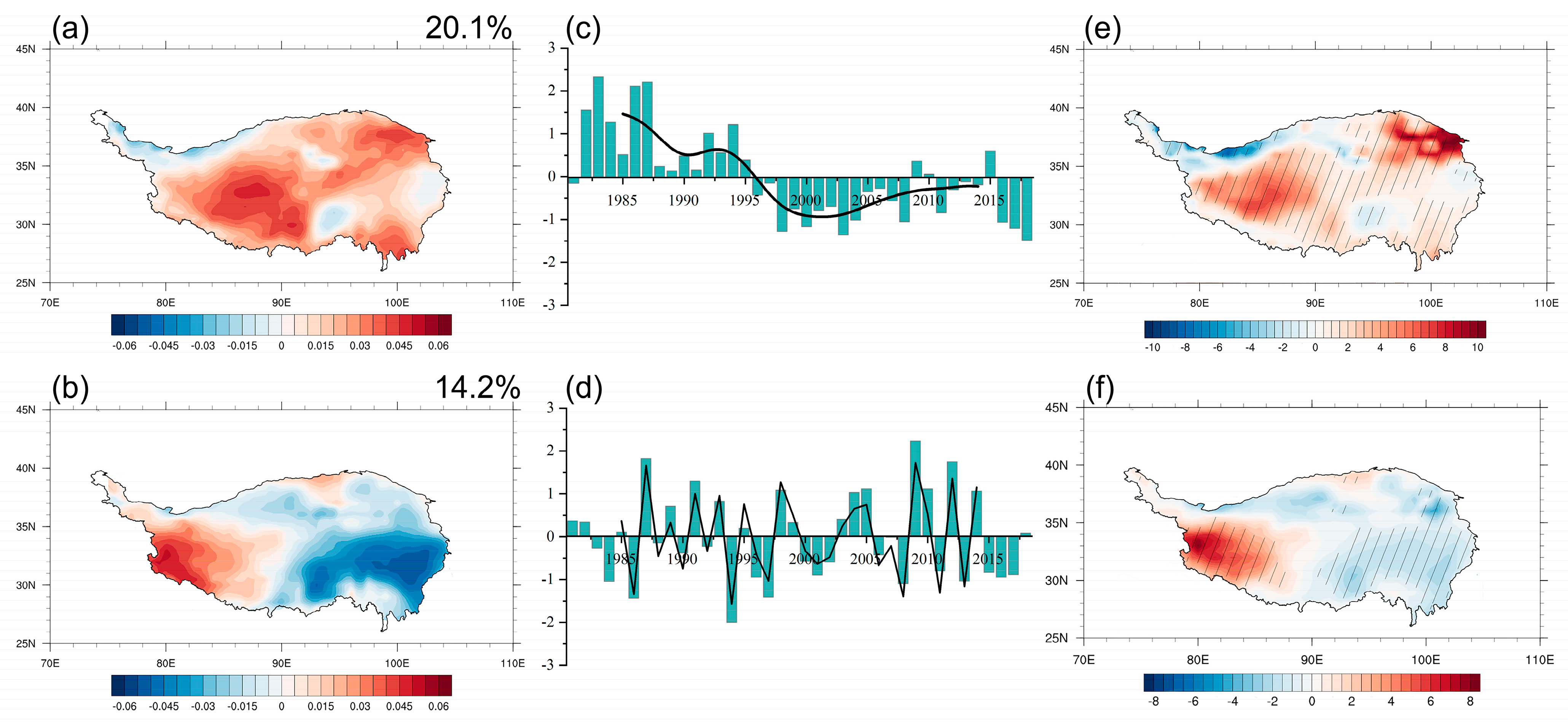
To identify the dominant modes of summer SH anomalies, EOF analysis was performed. The spatial distribution of the first dominant mode (EOF1) was marked by the consistent variations of summer SH over the whole TP, with an explained variance of 20.1% (Figure 2a). EOF1 was set apart from the other modes based on the North test. This means that EOF1 is considered statistically distinguishable and significant. Figure 2b shows the spatial distribution of EOF2. EOF2 accounted for 14.2% of the total variance and passed the North test [32]. A clear zonal seesaw pattern could be observed over the TP. The same analysis based on the remote sensing product derived from Han et al. [28,29] also indicated that the first leading mode of summer SH showed significant consistent variations, and the second leading mode of summer SH showed a zonal dipolar pattern (Figure S1).
Figure 2c shows the PC1 and its interdecadal component (PC1-ID). PC1-ID presented an interdecadal shift from the positive phase to the negative phase from around 1996. From the perspective of long-term trends, SH demonstrated reductions from the 1980s and a slight recovery from the 2000s, which is in agreement with previous studies [24,25]. The spatial distribution of the summer SH interdecadal component anomalies onto PC1-ID is shown in Figure 2e. Significant positive anomalies appeared in almost the entire TP, while weak negative anomalies occurred in the southeastern TP, which was similar to the first leading mode of SH driving from the EOF method, with a pattern correlation of up to 0.96 (Figure 2a). This indicates that the PC1-ID can effectively represent the interdecadal variation of summer SH over the TP.
Figure 2d shows the PC2 and its interannual component (PC2-IA). A remarkable feature of this was that the relation between PC2-IA and PC2 had a correlation coefficient of up to 0.95, which indicates that EOF2 presents the interannual variation of summer SH. The spatial distribution of SH anomalies associated with PC2-IA is shown in Figure 2f. A clear zonal seesaw pattern could be observed over the TP, with negative SH in the east of the TP and positive SH over the western TP. On the interannual time scale, when the PC2-IA was in a positive phase, SH over the TP exhibited a zonal asymmetric spatial mode with anomalous strengthening in SH over the western TP and anomalous weakening in SH over the eastern TP. Anomalies in the interannual component of SH associated with PC2-IA were the same as the second leading mode of SH derived from the EOF method (Figure 2b), which indicates that the EOF2 pattern can effectively represent the dominant mode of interannual variation in summer SH over the TP.

3.2. Physical Mechanisms of Variations in Summer SH

3.2.1. First Dominant Mode of Variation in Summer SH

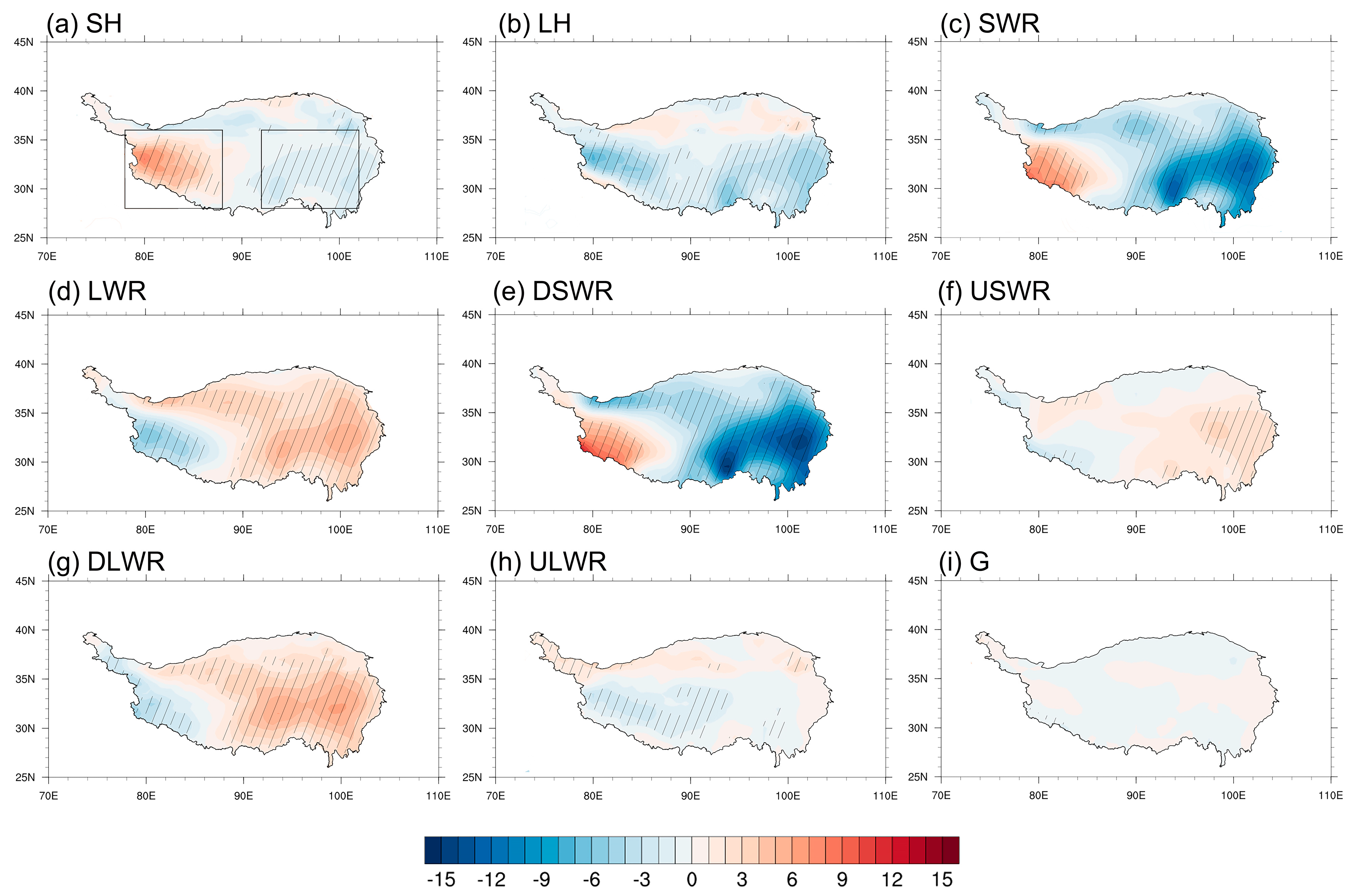
The first dominant mode of variation in summer SH presented an interdecadal weakening. As SH was determined by the local surface energy budget, the local surface energy budget related to anomalies in SH on the interdecadal time scale is investigated below. Considering SH experienced a decadal phase shift around 1996, we used the two periods, 1981–1995 and 1997–2018, to represent the decadal change in SH accordingly. Figure 3 presents the difference in surface fluxes between the two periods. Anomalies in SWR bore a close resemblance to the spatial pattern of SH with negative anomalies over the majority of the TP (Figure 3a,c). The anomalous decrease in SWR corresponded to significantly reduced DSWR over the TP (Figure 3e). This indicates that the DSWR has a positive contribution to the interdecadal variation of SH. The spatial distribution of anomalies in LWR presented strengthening over the TP (Figure 3d), which was dominated by the change in DLWR (Figure 3g). Moreover, the magnitude of anomalies in LH, USWR, ULWR, and G was too small to impact SH (Figure 3b,f,h,i). The contributions of the components to changes in SH are depicted in Figure 4. It was found that the first dominant mode of SH was mainly due to anomalous SWR induced by DSWR, while the LWR anomalies induced by DLWR helped to offset the decadal weakening of SH. The contribution of the other components was insignificant.
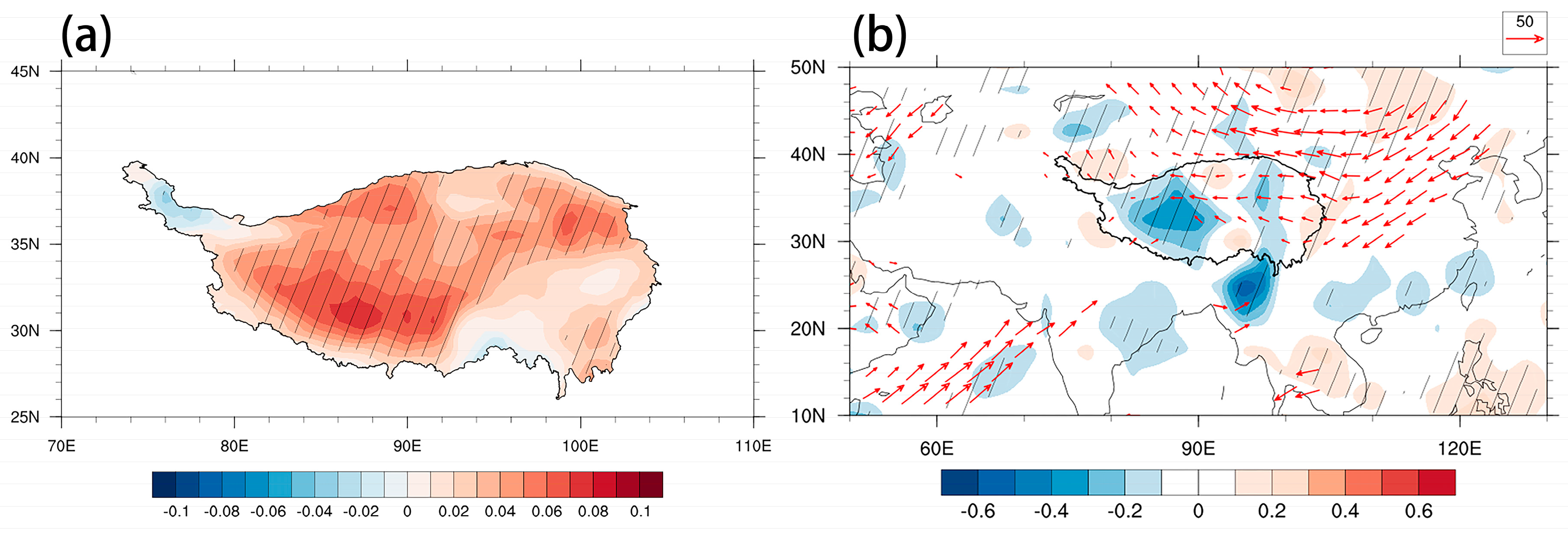
According to previous studies, cloud cover can regulate the DSWR and DLWR [33]. Therefore, the opposite variations of DSWR and DLWR may have been induced by the cloud cover. The total cloud cover variations associated with the interdecadal variation of SH were investigated next. Figure 5a displays the difference in the total cloud cover between 1997–2018 and 1981–1995. The TP was dominated by enhanced cloud cover, which induced more reflection of downwelling solar radiation and resulted in reduced DSWR. A decrease in DSWR can enhance SH owing to the surface energy budget. Figure 5b depicts the difference in water vapor flux and divergence between 1997–2018 and 1981–1995. A large westward water vapor flux emerged over the TP. This can enhance the convergence of water vapor flux over the TP by means of decreasing the water vapor exported from the eastern boundary of the TP. Associated with this increase in water vapor convergence, more summer cloud cover appeared over the TP (Figure 5a), inducing a decadal weakening of SH (Figure 3a).
Large-scale circulation anomalies can usually contribute to regional climatic change. Studying the impact of atmospheric circulation on TP SH can improve our understanding of climatic change over the TP, which is helpful for climate prediction. The atmospheric circulation anomalies linked to the interdecadal weakening of summer SH over the TP were examined further. Figure 6a displays the 500 hPa geopotential height and horizontal wind anomalies between 1997–2018 and 1981–1995. There was a wave train in the Eurasian continent. A considerably positive geopotential height center with an anticyclonic anomaly was located to the northeast of the TP, corresponding to this anomalous wave-like train. This led to a weakened subtropical westerly jet over the TP and less water vapor export from the eastern boundary of the TP. Figure 6b shows the 200 hPa geopotential height anomalies during the two periods. A zonal wave train occurred from the North Atlantic to the Eurasian continent, with two negative-height anomalies over the North Atlantic and West Asia and two positive-height anomalies over eastern Europe and Lake Baikal. The wave activity flux indicated that the wave train’s propagation direction was expected to be from the North Atlantic to the Eurasian continent. Such a circulation anomaly pattern is favorable for a reduced westerly jet and led to anomalous water vapor convergence of the TP (Figure 5b). This conclusion coincides with Zhou et al. [34], who proposed that the interdecadal variation in summer water vapor over the TP is related to a similar teleconnection pattern. Furthermore, the atmospheric circulation anomalies linked to PC1-ID were similar to those related to the interdecadal variation of SRP [35], implying that the SRP pattern may be crucial in the interdecadal variability of summer SH over the TP.

3.2.2. Second Dominant Mode of Variation in Summer SH

We next investigated the surface flux anomalies related to the second dominant mode of variation in TP summer SH. Figure 7 displays the surface flux anomalies related to the PC2-IA of summer SH. The upwelling surface longwave and shortwave radiations ranged from the surface to the atmosphere. In general, a large decrease in surface latent heating (LH) mainly appeared in the southern TP, and an insignificant increase occurred in the northern TP. Corresponding to the EOF2 of SH, a significant increase in the surface net shortwave radiation (SWR) was observed over the western TP and a remarkable reduction appeared in the eastern TP (Figure 7c). Anomalies in SWR were dominated by the zonally asymmetric pattern of downwelling surface shortwave radiation (DSWR) (Figure 7e). However, the contribution of upwelling surface shortwave radiation (USWR) to anomalies in SWR was insignificant (Figure 7f). This means that the DSWR has a positive contribution to anomalies in SH over the TP. On the contrary, anomalies of surface longwave radiation (LWR) (Figure 7d) mainly induced by anomalous downwelling surface longwave radiation (DLWR) (Figure 7g) negatively affected SH due to the opposite spatial pattern anomalies. Moreover, anomalies in upwelling surface longwave radiation (USWR) and the ground heat flux (G) were insignificant and had little impact on the change in SH.
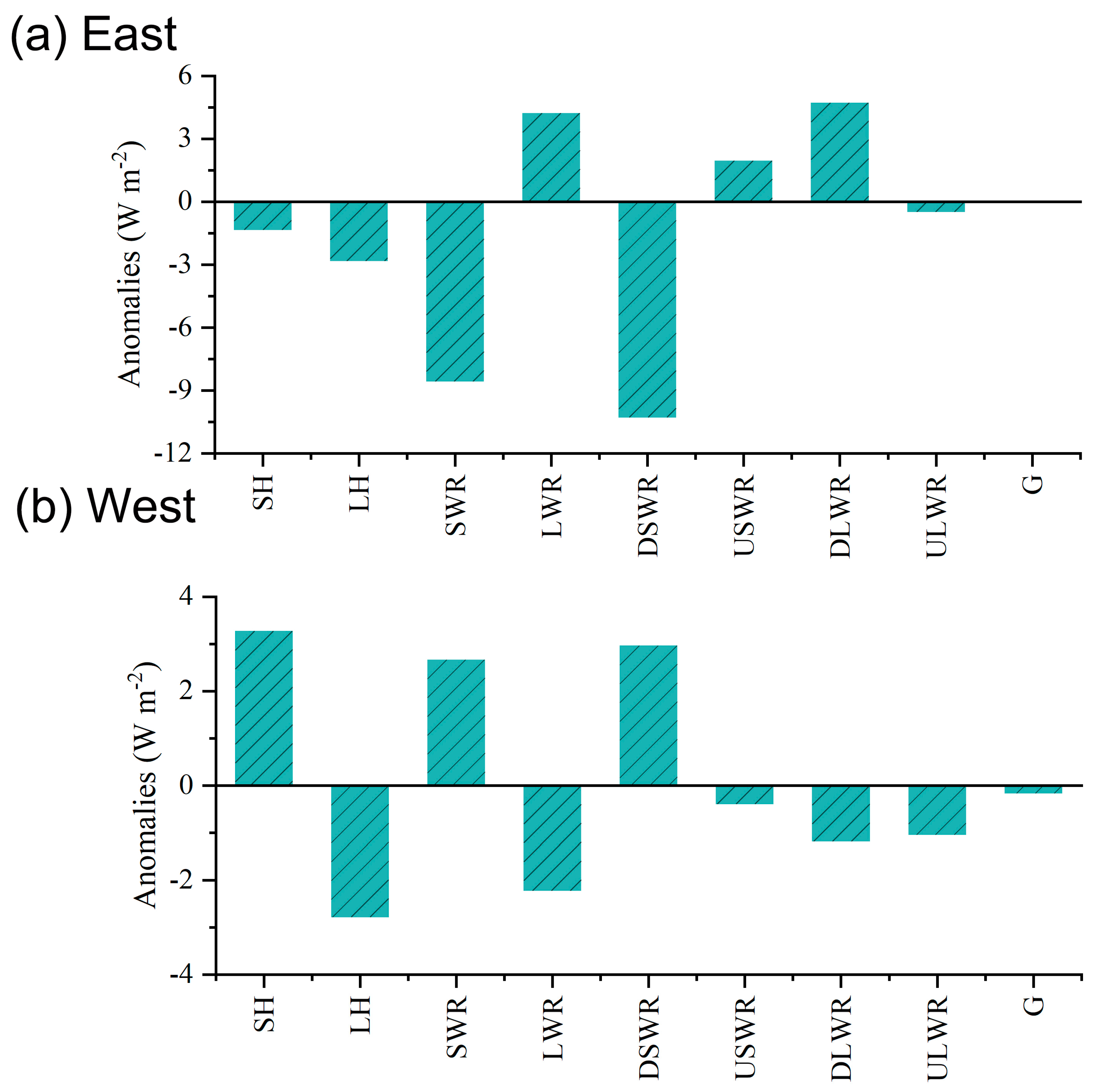
To further examine the contribution of each surface flux to SH anomalies, the average regional anomalies of SH, LH, SWR, LWR, DSWR, USWR, DLWR, ULWR, and G were calculated for the eastern TP (28–36° N, 78–88° E) (Figure 8a) and western TP (28–36° N, 92–102° E) (Figure 8b), respectively. For the eastern TP, a large decrease in SWR of approximately −9 W m−2 contributed to the decrease in SH and LH. The decrease in SWR is mainly attributed to the weakening of DSWR. For the western TP, enhanced SH was consistent with the increase in DSWR and decrease in LH, which means that the increase in SH was mainly due to DSWR and LH. The LWR presented a significant reduction of approximately −2.2 W m−2. Among the contributions to the SH change, the role of DSWR was predominant. Therefore, we investigated the role of DSWR in changing SH on the interannual time scale.
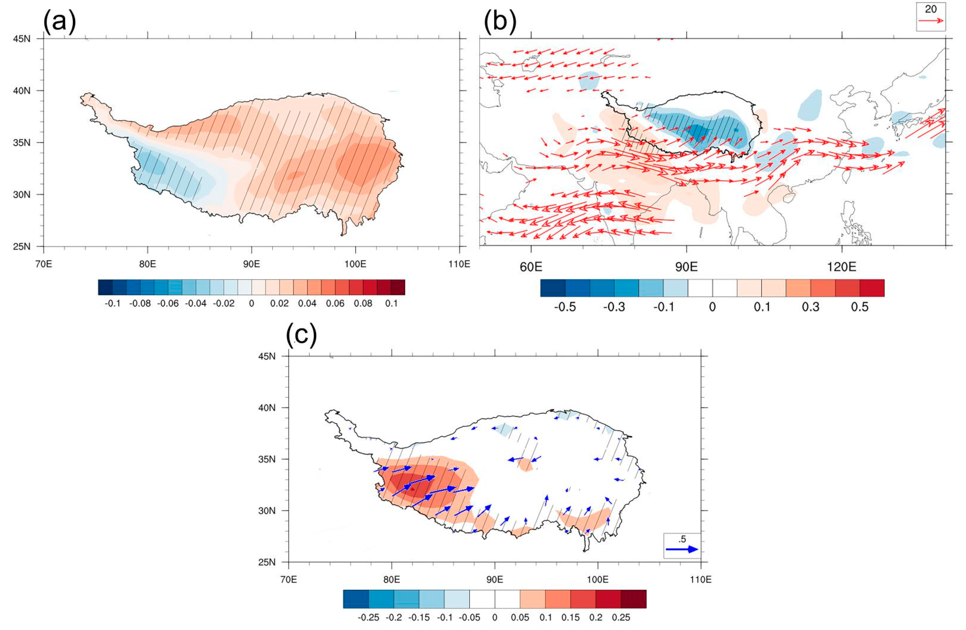
As investigated by previous studies [33], cloud cover has an important influence on the shortwave radiation reaching the surface. Figure 9a shows anomalies in total cloud cover related to the interannual variation of the TP summer SH. In contrast, less cloud cover appeared in the western TP, and more cloud cover appeared in the eastern TP. This indicates that the anomalous DSWR leading to the zonally asymmetric pattern of SH may be partly related to the variations of total cloud cover over the TP. Figure 9b presents the regression of water vapor flux and divergence onto PC2-IA. There was a significant southwesterly vapor supply from the Indian monsoon region to the main body of the TP, which was induced by the southwesterly anomalies. The anomalous water vapor flux divergence also presented a dipole mode with divergence in the west of the TP and convergence in the east of the TP. Sufficient moisture convergence (divergence) is favorable for the increase (decrease) in total cloud cover, and therefore induced weakened (enhanced) SH over the eastern (western) TP. According to previous studies, the variations of SH significantly respond to the changes in surface wind speed [17]. Figure 9c also displays the regression of the surface wind speed on PC2-IA. Remarkable southwesterly anomalies and positive surface wind speed anomalies were located in the western TP, in accordance with the anomalous enhancement in SH of the western TP (Figure 7a). This means that the positive SH of the western TP was also partly due to the strengthened surface wind speed, owing to the southwesterly wind anomalies.
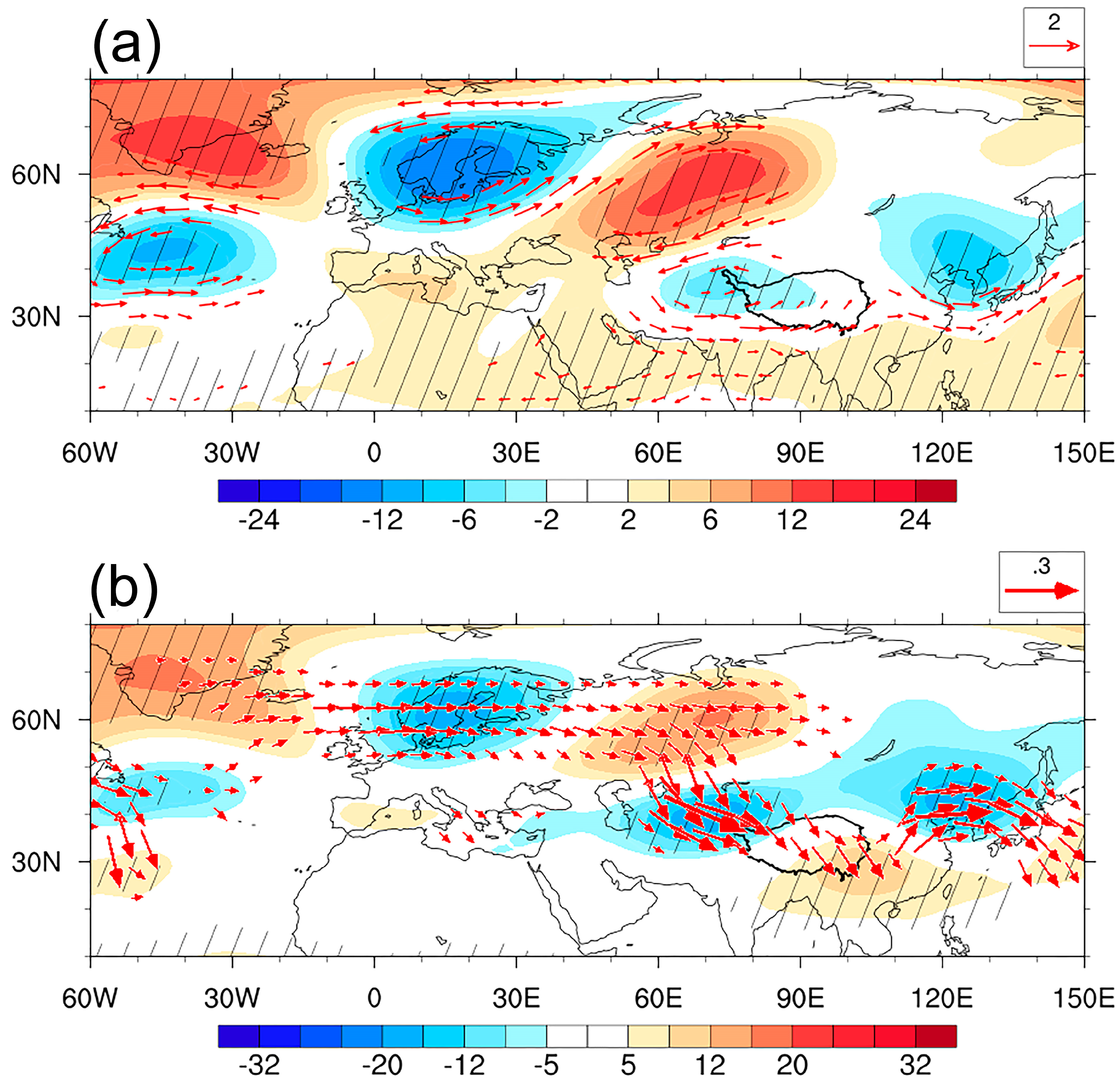
The above result indicates that interannual variation in SH can be mainly explained by the DSWR change, which is associated with moisture convergence and divergence. In addition, the southwesterly wind anomaly can also partly explain the SH anomalies in the western TP. These analyses suggest that atmospheric circulation changes may have an important impact on the SH anomalies by impacting the water vapor convergence and divergence and wind anomalies over the TP. Atmosphere circulation anomalies related to the anomalies in SH were further examined. Figure 10a displays 500 hPa geopotential height and horizontal wind anomalies related to the interannual variation of SH. An evident feature is that there was a significant, negative, high-pressure center to the west of the TP corresponding to the cyclonic anomaly, which led to enhanced southwest wind anomalies at the southwestern boundary of the TP and water vapor convergence (divergence) over the eastern (western) TP. Furthermore, 200 hPa geopotential height regressed against normalized PC2-IA presented a similar spatial pattern of 500 hPa, showing an equivalent barotropic structure in the vertical direction (Figure 10b). According to the horizontal wave activity flux, the teleconnection wave associated with SH anomalies originated in the North Atlantic and traveled eastward across the Eurasian continent. This suggests that atmospheric wave-like patterns originating in the North Atlantic may be important in the interannual variation of SH.

3.2.3. Association between Variations in Summer SH and Atmospheric Wave Trains

The above analysis indicated that the dominant modes of variations in summer SH over the TP had a close connection to atmospheric wave trains. Associations between variations in summer SH and atmospheric wave trains are investigated below.
We first investigated the impact of interdecadal variation in SRP on summer SH. According to previous studies [35,36,37], the SRP pattern is defined as the EOF1 of the summer mean 200 hPa meridional wind within the region 20–60° N, 0–150° E (Figure 11a), and the normalized PC1 is referred to as the SRP index (SRPI) (Figure 11b). A 9-year Lanczos low-pass filter was used to calculate the interdecadal component of SRPI (SRPI-ID), which can be seen in Figure 11c. The temporal correlation coefficient between PC1-ID and the SRPI-ID was up to 0.84, with a significance level of 99% (Figure 11c). Figure 11d shows the spatial distribution of SH anomalies related to the interdecadal variation of SRP. Significantly decreased anomalies occurred in almost the whole TP, while weak negative anomalies appeared in the southeastern TP. The spatial pattern was in good agreement with the distribution of interdecadal weakening of SH (Figure 3a). This suggests that the SRP is closely related to the interdecadal variability of SH. Figure 11e,f depict atmospheric circulation anomalies linked to SRP interdecadal variation. The 500 hPa geopotential height and horizontal wind anomalies regressed upon the SRPI-ID multiplied by −1 are presented in Figure 11e. To the northeast of the TP, significant positive height anomalies arose, which were related to the decadal weakening of SH. The anomalous positive height accompanied the anticyclonic anomaly to the northeast of the TP. In relation to the anticyclonic circulation at 500 hPa, easterly wind anomalies to the south of the anticyclonic center flowed into the TP from the eastern boundary of the TP, resulting in a diminished subtropical westerly jet. Corresponding to the easterly anomalies there was significant water vapor convergence and enhanced cloud cover, which could reduce DSWR and SH in the TP. The above analysis indicated that the interdecadal variation of SRP can significantly induce anomalous weakening in SH over the TP by impacting the circulation anomalies and, therefore, cloud cover and DSWR anomalies.
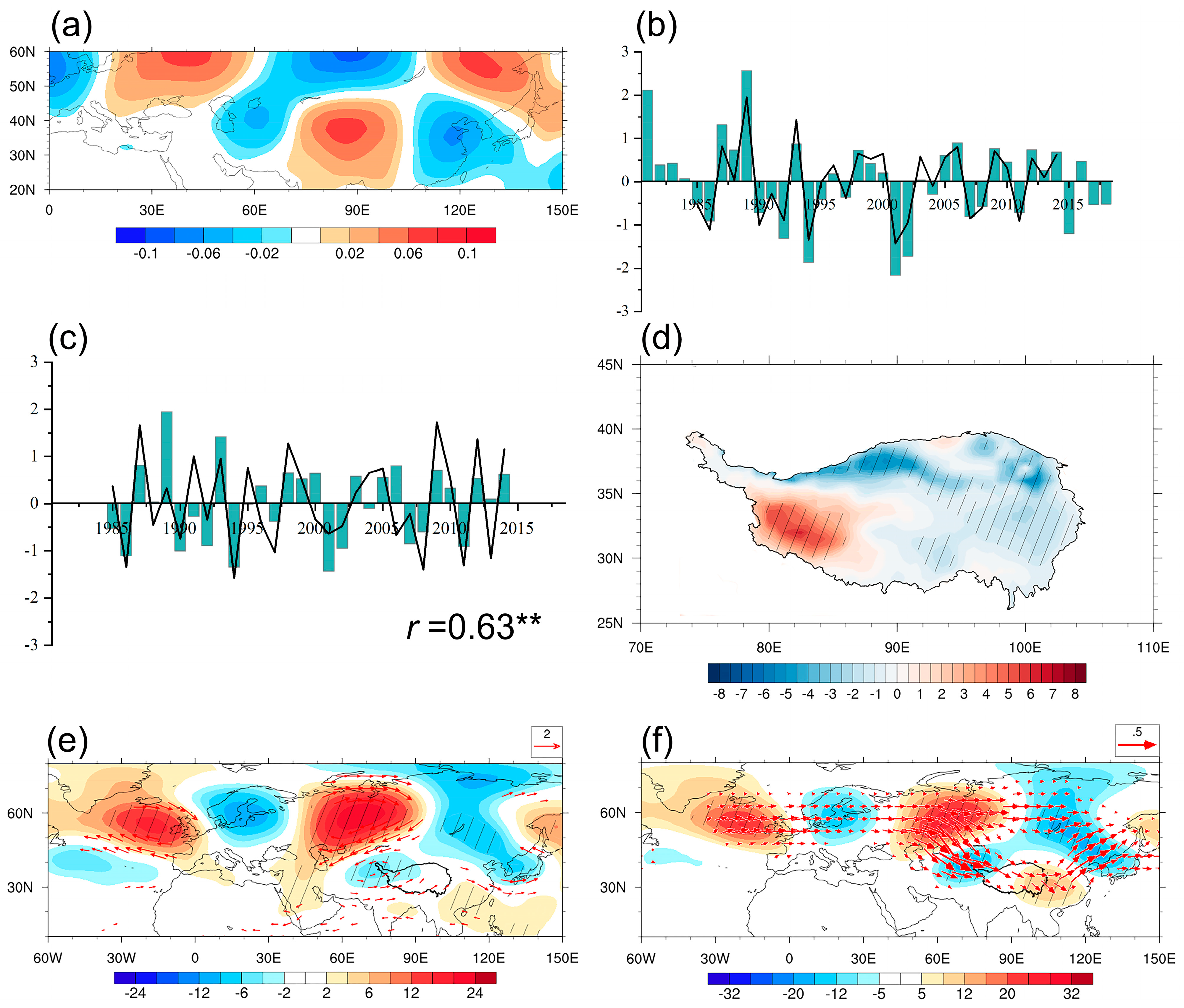
We also found that the second leading mode of the upper-tropospheric 200 hPa meridional wind anomalies in 20–60° N, 0–150° E during summer, which is defined as the North Atlantic-East and North Asia pattern (NAENA), had significant impacts on the interannual variation of SH (Figure 12a). The NAENA index (NAENAI) is defined as the PC2 corresponding to EOF2 of the summer 200 hPa meridional wind over the Eurasian continent (Figure 12b). Figure 12c displays the normalized time series of the interannual component of NAENAI (NAENAI-IA) (column) and PC2-IA (black line). The temporal correlation coefficient between PC2-IA and NAENAI-IA during the period of 1981–2018 was up to 0.63, which indicated that the interannual variation in NAENA could explain approximately 40% of the anomalies in summer SH on the interannual time scale. Figure 12d shows anomalies in SH obtained by regression upon NAENAI. Positive SH anomalies predominated in the west of the TP, whereas weakened SH anomalies arose in the east of the TP, resembling the spatial pattern of EOF2 (Figure 2b). Moreover, the spatial pattern of NAENA showed close similarity to the atmospheric circulation anomalies associated with the interannual variation of SH (Figure 12e,f). The above analysis suggested that NAENA can impact the interannual variation of summer SH over the TP by means of changing the wind speed and water vapor convergence and divergence over the TP.

4. Discussion

Summer SH over the TP had a significant influence on the regional and Asian climate. Therefore, comprehending and predicting the variability of summer SH is of great importance. Using the monthly remote sensing and reanalysis data with a period of 2001–2018, the features of dominant modes of SH were investigated in this study. EOF analysis showed that an interdecadal weakening of SH appeared over almost the whole TP from 1981–2018 in the leading mode. This is in great agreement with previous studies. Duan et al. [17] indicated that SH over the TP exhibited a decreasing trend since the 1980s, which was mainly induced by the weakening of the westerly jet. In recent years, SH has presented an increasing trend as the result of enhanced surface wind speed [18,38]. However, it was thought that the variations of SH were long-term trends due to global warming and its hiatus, while this study considered that the different trends of SH might be a manifestation of the interdecadal variation. Based on satellite data and observations, recent studies [23] have found that SH has increased slightly over the TP from around 2001. To reach more accurate SH over the TP, the introduction of satellite data will be carried out in the future, which would overcome the shortage of accuracy in reanalysis data. The EOF2 pattern of summer SH over the TP was characterized by a zonally asymmetric pattern with positive (negative) SH anomalies in the western (eastern) TP. This indicated that positive SH anomalies in the western TP are usually accompanied by negative SH anomalies in the eastern TP on an interannual time scale. Based on meteorological data and satellite products, a recent study found that the long-term variations of summer evapotranspiration (ET) over the TP present a dipole pattern, with an increasing trend in the eastern TP and a decreasing trend in the western TP [29]. It is worth studying the cause of opposite spatial patterns between SH and ET over the TP.
Further analysis showed that the interannual variation of SH had a tight connection to the stationary teleconnection pattern NAENA, which was the second leading mode of the upper-tropospheric meridional wind anomalies over the Eurasian continent in summer. The interdecadal weakening of summer SH over the TP was mainly due to the decreased westerly wind anomalies over the TP, which were induced by the anticyclonic circulation to the northeast of the TP. The atmospheric circulation anomalies linked to the interdecadal weakening of SH were characterized by a teleconnection wave train, which was similar to that linked to the interdecadal phase shift of SRP. This indicated that the decadal shift of the phase in SRP plays a crucial role in the interdecadal weakening of SH. Han et al. [38] suggested that SRP is a key factor influencing summer atmospheric heat over the inner TP on interdecadal time scales, which is consistent with our conclusion. A recent study proposed that the predictability of the TP rainfall also originates from SRP [39]. Therefore, the interdecadal variation of SRP can significantly impact the climate variations of the TP on interdecadal and multidecadal time scales and acts as a potential predictor for the climate variations for TP. Previous studies have demonstrated that the phase of the AMO is likely to provide some prediction potential for the interdecadal variations of SRP [35]. The impacts of mid-high atmospheric circulation systems on the TP call for further studies.

5. Conclusions

This study examined the dominant modes of variability in summer SH over the TP based on reanalysis and remote sensing data. The role of atmospheric teleconnection patterns in SH was also investigated. The main conclusions are as follows:
(1)
The large value area in SH and its standard deviation was concentrated in the north and west of the TP. The first leading mode of the TP summer SH during the period 1981–2018 presented a decadal shift from a positive phase to a negative phase after around 1996. The second leading mode was characterized by a zonal dipole pattern with enhanced (weakened) SH anomalies in the western (eastern) TP on the interannual time scale.
(2)
The interannual variation of summer SH was dominated by anomalies in DSWR, which was associated with the anomalous cloud cover over the TP. An atmospheric pattern referred to as NAENA induced an anticyclone anomaly to the west of the TP, leading to anomalous water vapor convergence (divergence) and more (less) cloud cover in the eastern (western) TP. Corresponding to the increase (decrease) in cloud cover, DSWR presented anomalous enhancement (reduction) and resulted in a zonal dipole pattern with strengthened (weakened) SH in the western (eastern) TP.
(3)
Interdecadal weakening of summer SH was associated with the interdecadal variation of DSWR induced by the enhancement of cloud cover. The decadal change in cloud cover over the TP was mainly due to the variation of water vapor transport as a result of the decadal phase shift of SRP. An anticyclone circulation to the northeast of the TP associated with SRP led to enhanced water vapor supply and convergence of the TP, which resulted in an increase in cloud cover and a reduction in DSWR, contributing to the interdecadal decrease in SH over the TP.
By investigating the relationship between large-scale circulation and the TP thermodynamic forcing, this study is crucial for us to understand the land-atmosphere interaction and its climatic effects of the TP.

Supplementary Materials

The following supporting information can be downloaded at: https://www.mdpi.com/article/10.3390/rs14040956/s1, Figure S1: The first two EOFs of summer SH over the TP for the period 2001–2018 derived from ERA-Interim (a,d) and remote sensing data (b,e). Normalized time series of PC1 (c) and PC2 (f) derived from ERA-Interim (black line) and remote sensing data (red line).

Author Contributions

Conceptualization, Z.H.; methodology, W.F. and C.H.; software, W.F.; investigation, W.F. and Z.H.; writing—original draft preparation, W.F., X.H., Y.Y. and H.Y.; writing—review and editing, W.F., Z.H., W.M., Y.M., C.H., D.W. and C.F. All authors have read and agreed to the published version of the manuscript.

Funding

This research was supported by the Second Tibetan Plateau Scientific Expedition and Research (STEP) program (grant no. 2019QZKK0103), the National Natural Science Foundation of China (grant no. 91837208, 41830650), the Strategic Priority Research Program of Chinese Academy of Sciences (grant no. XDA20060101) and the National Key Research and Development Program of China (grant no. 2018YFC1505701).

Institutional Review Board Statement

Not applicable.

Informed Consent Statement

Not applicable.

Data Availability Statement

The ERA-Interim reanalysis from the ECMWF used in this study can be accessed online (https://www.ecmwf.int/en/forecasts/datasets/reanalysis-datasets/ (accessed on 1 January 2022)). The NCEP/NCAR reanalysis used in this study can be accessed at https://psl.noaa.gov/data/reanalysis/reanalysis.shtml (accessed on 1 January 2022). The CRU dataset can be accessed at https://data.ceda.ac.uk/ (accessed on 5 January 2022).

Conflicts of Interest

The authors declare no conflict of interest.

References

  1. Xu, X.; Lu, C.; Shi, X.; Gao, S. World water tower: An atmospheric perspective. Geophys. Res. Lett. 2008, 35, L20815. [Google Scholar] [CrossRef]
  2. Kang, S.; Xu, Y.; You, Q.; Flügel, W.A.; Pepin, N.; Yao, T. Review of climate and cryospheric change in the Tibetan Plateau. Environ. Res. Lett. 2010, 5, 015101. [Google Scholar] [CrossRef]
  3. Wang, B.; Ma, Y.; Su, Z.; Wang, Y.; Ma, W. Quantifying the evaporation amounts of 75 high-elevation large dimictic lakes on the Tibetan Plateau. Sci. Adv. 2020, 6, eaay8558. [Google Scholar] [CrossRef] [PubMed]
  4. Zhao, Y.; Zhou, T. Asian water tower evinced in total column water vapor: A comparison among multiple satellite and reanalysis data sets. Clim. Dyn. 2020, 54, 231–245. [Google Scholar] [CrossRef] [Green Version]
  5. Cuo, L.; Zhang, Y.; Zhu, F.; Liang, L. Characteristics and changes of streamflow on the Tibetan Plateau: A review. J. Hydrol. Reg. Stud. 2014, 2, 49–68. [Google Scholar] [CrossRef] [Green Version]
  6. Xu, X.; Zhao, T.; Lu, C.; Guo, Y.; Chen, B.; Liu, R.; Li, Y.; Shi, X. An important mechanism sustaining the atmospheric “water tower” over the Tibetan Plateau. Atmos. Chem. Phys. 2014, 14, 11287–11295. [Google Scholar] [CrossRef] [Green Version]
  7. Yanai, M.; Li, C. Mechanism of heating and the boundary layer over the Tibetan Plateau. Mon. Weather Rev. 1994, 122, 305–323. [Google Scholar] [CrossRef]
  8. Wu, G.; Zhang, Y. Tibetan Plateau forcing and the timing of the monsoon onset over South Asia and the South China Sea. Mon. Weather Rev. 1998, 126, 913–927. [Google Scholar] [CrossRef]
  9. Wu, G.; Liu, Y.; Zhang, Q.; Duan, A.; Wang, T.; Wan, R.; Liu, X.; Li, W.; Zhang, Z.; Wang, Z.; et al. The influence of mechanical and thermal forcing by the Tibetan Plateau on Asian climate. J. Hydrometeorol. 2007, 8, 770–789. [Google Scholar] [CrossRef] [Green Version]
  10. Li, L.; Zhang, R.; Wen, M.; Liu, L. Effect of the atmospheric heat source on the development and eastward movement of the Tibetan Plateau vortices. Tellus A Dyn. Meteorol. Oceanogr. 2014, 66, 24451. [Google Scholar] [CrossRef] [Green Version]
  11. Yanai, M.; Li, C.; Song, Z. Seasonal heating of the Tibetan Plateau and its effects on the evolution of the Asian summer monsoon. J. Meteorol. Soc. Japan. Ser. II 1992, 70, 319–351. [Google Scholar] [CrossRef] [Green Version]
  12. Duan, A.; Li, F.; Wang, M.; Wu, G. Persistent weakening trend in the spring sensible heat source over the Tibetan Plateau and its impact on the Asian summer monsoon. J. Clim. 2011, 24, 5671–5682. [Google Scholar] [CrossRef] [Green Version]
  13. Ye, D.; Wu, G. The role of the heat source of the Tibetan plateau in the general circulation. Meteorol. Atmos. Phys. 1998, 67, 181–198. [Google Scholar] [CrossRef]
  14. Hsu, H.; Liu, X. Relationship between the Tibetan Plateau heating and East Asian summer monsoon rainfall. Geophys. Res. Lett. 2013, 30, 2066. [Google Scholar] [CrossRef] [Green Version]
  15. Wang, Z.; Duan, A.; Wu, G. Time-lagged impact of spring sensible heat over the Tibetan Plateau on the summer rainfall anomaly in East China: Case studies using the WRF model. Clim. Dyn. 2014, 42, 2885–2898. [Google Scholar] [CrossRef]
  16. Xie, X.; Duan, A.; Shi, Z.; Li, X.; Sun, H.; Liu, X.; Cheng, X.; Zhao, T.; Che, H.; Liu, Y. Modulation of springtime surface sensible heating over the Tibetan Plateau on the interannual variability of East Asian dust cycle. Atmospheric Chemistry and Physics. 2020, 20, 11143–11159. [Google Scholar] [CrossRef]
  17. Duan, A.; Wu, G. Weakening trend in the atmospheric heat source over the Tibetan Plateau during recent decades. Part I: Observations. J. Clim. 2008, 21, 3149–3164. [Google Scholar] [CrossRef] [Green Version]
  18. Zhu, L.; Huang, G.; Fan, G.; Qu, X.; Zhao, G.; Hua, W. Evolution of surface sensible heat over the Tibetan Plateau under the recent global warming hiatus. Adv. Atmos. Sci. 2017, 34, 1249–1262. [Google Scholar] [CrossRef]
  19. Wang, M.; Wang, J.; Chen, D.; Duan, A.; Liu, Y.; Zhou, S.; Guo, D.; Wang, H.; Ju, W. Recent recovery of the boreal spring sensible heating over the Tibetan Plateau will continue in CMIP6 future projections. Environ. Res. Lett. 2019, 14, 124066. [Google Scholar] [CrossRef] [Green Version]
  20. Zhu, L.; Huang, G.; Fan, G.; Qü, X.; Wang, Z.; Hua, W. Elevation-dependent sensible heat flux trend over the Tibetan Plateau and its possible causes. Clim. Dyn. 2019, 52, 3997–4009. [Google Scholar] [CrossRef]
  21. Cui, Y.; Duan, A.; Liu, Y.; Wu, G. Interannual variability of the spring atmospheric heat source over the Tibetan Plateau forced by the North Atlantic SSTA. Clim. Dyn. 2015, 45, 1617–1634. [Google Scholar] [CrossRef]
  22. Yu, W.; Liu, Y.; Yang, X.; Wu, G.; He, B.; Li, J.; Bao, Q. Impact of North Atlantic SST and Tibetan Plateau forcing on the seasonal transition of springtime South Asian monsoon circulation. Clim. Dyn. 2021, 56, 559–579. [Google Scholar] [CrossRef]
  23. Ma, Y.; Wang, Y.; Han, C. Regionalization of land surface heat fluxes over the heterogeneous landscape: From the Tibetan Plateau to the Third Pole region. Int. J. Remote Sens. 2018, 39, 5872–5890. [Google Scholar] [CrossRef]
  24. Qian, Y.; Zhang, Y.; Huang, Y.; Huang, Y.; Yao, Y. The effects of the thermal anomalies over the Tibetan Plateau and its vicinities on climate variability in China. Adv. Atmos. Sci. 2004, 21, 369–381. [Google Scholar]
  25. Chen, B.; Qian, Z.; Zhang, L. Numerical simulation of formation and development of vortices over the Qinghai-Xizang Plateau in summer. Chin. J. Atmos. Sci. 1996, 20, 491–502. [Google Scholar]
  26. Liang, L.; Li, Y.; Hu, H.; Jiang, X.; Zhang, E. Numerical study of the influence of sensible heat anomalies in summer over Qinghai-Xizang Plateau on rainfall in Sichuan-Chongqing regions. Plateau Meteorol. 2013, 32, 1538–1545. (In Chinese) [Google Scholar]
  27. Yang, Y.; Liu, Y.; Li, M.; Hu, Z.; Ding, Z. Assessment of reanalysis flux products based on eddy covariance observations over the Tibetan Plateau. Theor. Appl. Climatol. 2019, 138, 275–292. [Google Scholar] [CrossRef]
  28. Han, C.; Ma, Y.; Chen, X.; Su, Z. Trends of land surface heat fluxes on the Tibetan Plateau from 2001 to 2012. Int. J. Climatol. 2017, 37, 4757–4767. [Google Scholar] [CrossRef]
  29. Han, C.; Ma, Y.; Wang, B.; Zhong, L.; Ma, W.; Chen, X.; Su, Z. Long-term variations in actual evapotranspiration over the Tibetan Plateau. Earth Syst. Sci. Data 2021, 13, 3513–3524. [Google Scholar] [CrossRef]
  30. Su, Z. The Surface Energy Balance System (SEBS) for estimation of turbulent heat fluxes. Hydrol. Earth Syst. Sci. 2002, 6, 85–100. [Google Scholar] [CrossRef]
  31. Takaya, K.; Nakamura, H. A formulation of a phase-independent wave-activity flux for stationary and migratory quasigeostrophic eddies on a zonally varying basic flow. J. Atmos. Sci. 2001, 58, 608–627. [Google Scholar] [CrossRef]
  32. North, G.; Bell, T.; Cahalan, R.; Moeng, F.J. Sampling errors in the estimation of empirical orthogonal functions. Mon. Weather Rev. 1982, 110, 699–706. [Google Scholar] [CrossRef]
  33. Chen, S.; Wu, R.; Liu, Y. Dominant modes of interannual variability in Eurasian surface air temperature during boreal spring. J. Clim. 2016, 29, 1109–1125. [Google Scholar] [CrossRef]
  34. Zhou, C.; Zhao, P.; Chen, J. The interdecadal change of summer water vapor over the Tibetan Plateau and associated mechanisms. J. Clim. 2019, 32, 4103–4119. [Google Scholar] [CrossRef]
  35. Wang, L.; Xu, P.; Chen, W.; Liu, Y. Interdecadal variations of the Silk Road pattern. J. Clim. 2017, 30, 9915–9932. [Google Scholar] [CrossRef]
  36. Li, X.; Lu, R.; Ahn, J.B. Combined effects of the British-Baikal Corridor pattern and the Silk Road pattern on Eurasian surface air temperatures in summer. J. Clim. 2021, 34, 3707–3720. [Google Scholar] [CrossRef]
  37. Han, Y.; Ma, W.; Yang, Y.; Ma, Y.; Xie, Z.; Sun, G.; Menenti, M.; Su, B. Impacts of the Silk Road pattern on the interdecadal variations of the atmospheric heat source over the Tibetan Plateau. Atmos. Res. 2021, 260, 105696. [Google Scholar] [CrossRef]
  38. Fan, W.; Ma, W.; Hu, Z.; Ma, Y. Recovery of sensible heating and its elevation amplification over and around the Tibetan Plateau since the 2000s. Theor. Appl. Climatol. 2021, 146, 617–630. [Google Scholar] [CrossRef]
  39. Hu, S.; Zhou, T. Skillful prediction of summer rainfall in the Tibetan Plateau on multiyear time scales. Sci. Adv. 2021, 7, eabf9395. [Google Scholar] [CrossRef]
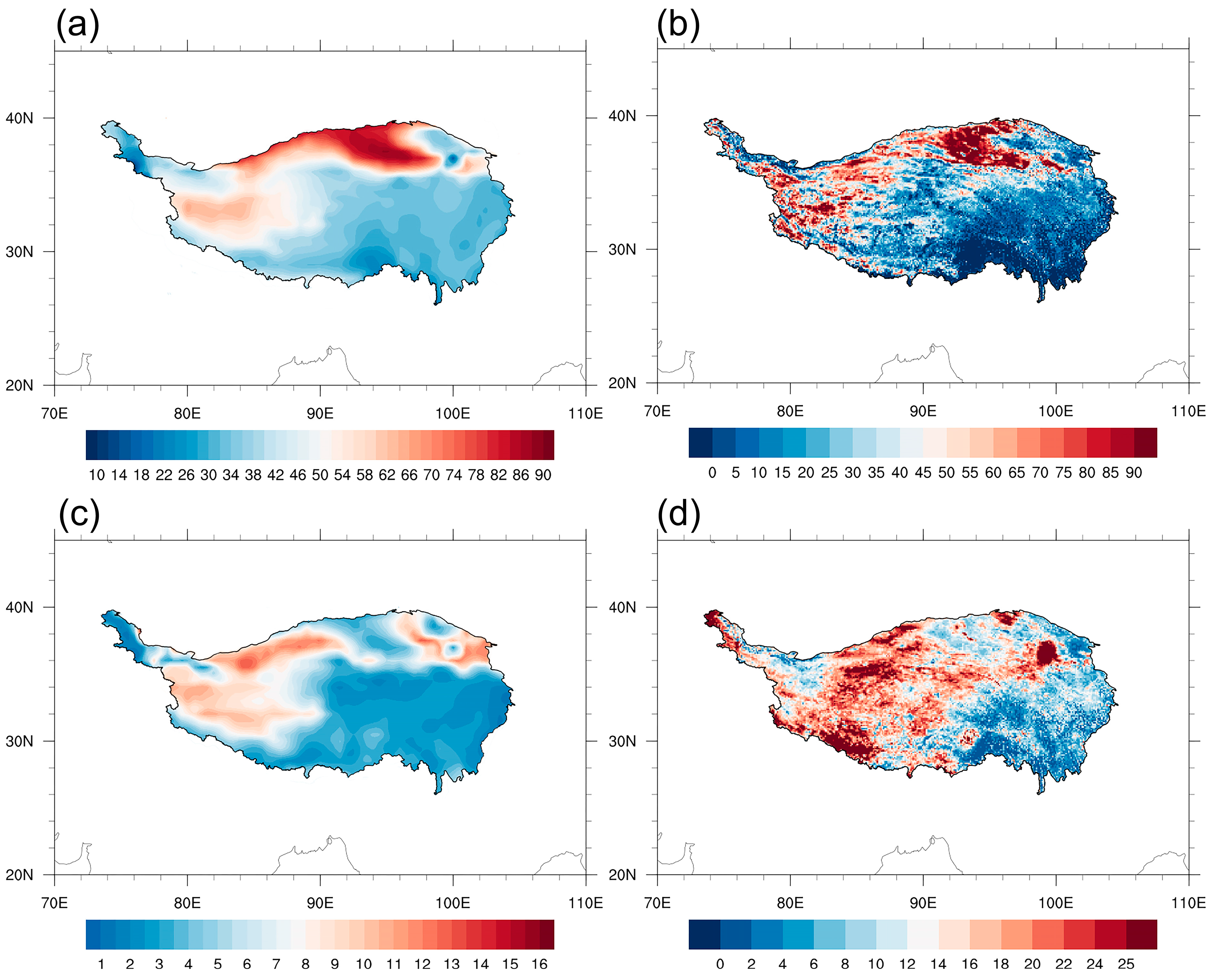
Figure 1. The spatial pattern of the TP summer SH climatology (W m−2) from ERA-Interim (a) and remote sensing product derived from Han et al. [28,29] (b), standard deviation (W m−2) from ERA-Interim reanalysis (c), and remote sensing (d) data.
Remotesensing 14 00956 g001
Figure 2. The first two EOFs of summer SH over the TP for the period 1981–2018 (a,b). The explained variance of EOF is in the upper right of (a,b). Normalized time series of PC1 (column) and its interdecadal component (PC1-ID) (line) (c). Normalized time series of PC2 (column) and its interannual component (PC2-IA) (line) (d). Regression of the interdecadal component of summer SH (shading, W m−2) on PC1-ID (e). Regression of the interannual component of summer SH (shading, W m−2) on PC2-IA (f). Grid points with statistically significant anomalies passing the 95% confidence level are denoted by an oblique line.
Remotesensing 14 00956 g002
Figure 3. Spatial distribution of difference in sensible heating (SH) (a), latent heating (LH) (b), surface net shortwave radiation (SWR) (c), surface net longwave radiation (LWR) (d), downwelling surface shortwave radiation (DSWR) (e), upwelling surface shortwave radiation (USWR) (f), downwelling surface longwave radiation (DLWR) (g), upwelling surface longwave radiation (ULWR) (h), and ground heating (G) (i) between 1997–2018 and 1981–1995 (shading, W m−2). Grid points with statistically significant anomalies passing the 95% confidence level are denoted by an oblique line.
Remotesensing 14 00956 g003
Figure 4. The difference in SH, LH, SWR, LWR, DSWR, LSWR, DLWR, ULWR, and G between 1997–2018 and 1981–1995 over the TP (W m−2).
Remotesensing 14 00956 g004
Figure 5. Spatial distribution of difference in total cloud cover (a), water vapor flux exceeding the 95% confidence level (vector, kg m−1 s−1), and divergence (shading, 10−4 kg m−2 s−1) (b) between 1997–2018 and 1981–1995. Grid points with statistically significant anomalies passing the 95% confidence level are denoted by oblique lines.
Remotesensing 14 00956 g005
Figure 6. Spatial distribution of difference in 500 hPa geopotential height anomalies (shading, gpm) and the wind exceeding the 95% confidence level (vector, m s1) (a), the 200 hPa geopotential height anomalies (shading, gpm), and the wave activity flux (vector, m2 s−2) (b) between 1997–2018 and 1981–1995. Grid points with statistically significant anomalies passing the 95% confidence level are denoted by oblique lines.
Remotesensing 14 00956 g006
Figure 7. Anomalies in the interannual component of SH (a), LH (b), SWR (c), LWR (d), DSWR (e), LSWR (f), DLWR (g), ULWR (h), and G (i) regressed on PC2-IA (shading, W m−2). Grid points with statistically significant anomalies passing the 95% confidence level are denoted by oblique lines. The two black rectangles denote the western TP (28–36° N, 78–88° E) and eastern TP (28–36° N, 92–102° E).
Remotesensing 14 00956 g007
Figure 8. Anomalies in the interannual component of SH, LH, SWR, LWR, DSWR, LSWR, DLWR, ULWR, and G regressed on PC2-IA (W m−2) in the region of eastern TP (a) and western TP (b).
Remotesensing 14 00956 g008
Figure 9. Anomalies in the interannual component of total cloud cover (a), water vapor flux exceeding the 95% confidence level (vector, kg m−1 s−1) and divergence (shading, 10−4 kg m−2 s−1) (b), surface wind vectors passing the 95% confidence level (vector, m s−1), and wind speed (shading, m s−1) (c) regressed on PC2-IA. Grid points with statistically significant anomalies passing the 95% confidence level are denoted by an oblique line.
Remotesensing 14 00956 g009
Figure 10. Anomalies in the interannual component of 500 hPa geopotential height (shading, gpm) and wind passing the 95% confidence level (vector, m/s) (a), the 200 hPa geopotential height (shading, gpm), and the wave activity flux (vector, m2 s−2) (b) regressed on PC2-IA. Grid points with statistically significant anomalies passing the 95% confidence level are denoted by oblique lines.
Remotesensing 14 00956 g010
Figure 11. (a) The first EOF of summer means 200 hPa meridional wind over the region 20–60° N, 0–150° E for the period 1981–2018. (b) Normalized time series of SRPindex (column) and its interdecadal component (line). (c) Normalized time series of interdecadal component of SRP index (column) and PC1-ID (line). (**: significant at 99% confidience level). Anomalies in the interdecadal component of sensible heating (d), 500 hPa geopotential height (shading, gpm) and the wind exceeding the 95% confidence level (vector, m/s) (e), the 200 hPa geopotential height (shading, gpm) (f) regressed on SRPI-ID multiplied by −1. Grid points with statistically significant anomalies passing the 95% confidence level are denoted by oblique lines.
Remotesensing 14 00956 g011
Figure 12. (a) The second EOF of summer mean 200 hPa meridional wind in 20–60° N, 0–150° E for the period 1981–2018. (b) Normalized time series of NAENA index (column) and its interannual component (line). (c) Normalized time series of interannual components of NAENAI (column) and PC2-IA (line), (**: significant at 99% confidience level). Anomalies in the interannual component of sensible heating (d), 500 hPa geopotential height (shading, gpm) and the wind exceeding the 95% confidence level (vector, m/s) (e), the 200 hPa geopotential height (shading, gpm), and the wave activity flux (vector, m2 s−2) (f) regressed on PC2-IA. Grid points with statistically significant anomalies passing the 95% confidence level are denoted by oblique lines.
Remotesensing 14 00956 g012
Table 1. Summary of the datasets used in the study.
VariablesData SourceAvailabilityTemporal ResolutionSpatial Resolution
Sensible heat flux
(Reanalysis)
ERA-Interim1981–2018Daily0.5° × 0.5°
Sensible heat flux
(Remote Sensing)
Han et al. [28,29]2001–2018Monthly0.1° × 0.1°
Surface wind speed
Total cloud cover
Latent heat flux
Surface radiation
ERA-Interim1981–2018Monthly0.5° × 0.5°
Geopotential height
Zonal wind
Meridional wind
NCEP/NCAR1981–2018Monthly2.5° × 2.5°
Publisher’s Note: MDPI stays neutral with regard to jurisdictional claims in published maps and institutional affiliations.