Article

The Determination of the Snow Optical Grain Diameter and Snowmelt Area on the Greenland Ice Sheet Using Spaceborne Optical Observations

by
Baptiste Vandecrux
1,*,
Jason E. Box
1,
Adrien Wehrlé
1,2,
Alexander A. Kokhanovsky
3,
Ghislain Picard
4,
Masashi Niwano
5,
Maria Hörhold
6,
Anne-Katrine Faber
7 and
Hans Christian Steen-Larsen
7
1
Geological Survey of Denmark and Greenland (GEUS), 1350 Copenhagen, Denmark
2
Institute of Geography, University of Zurich, 8057 Zurich, Switzerland
3
Telespazio Belgium, Bratustrasse 7, 64295 Darmstadt, Germany
4
Institut des Géosciences de l’Environnement (IGE), Université Grenoble Alpes, CNRS, UMR 5001, 38041 Grenoble, France
5
Physical Meteorology Research Department, Meteorological Research Institute, Tsukuba 305-0052, Japan
6
Alfred-Wegener-Institut, Helmholtz-Zentrum für Polar-und Meeresforschung, Am Handelshafen 12, 27570 Bremerhaven, Germany
7
Geophysical Institute, Bjerknes Centre for Climate Research, University of Bergen, 5020 Bergen, Norway
*
Author to whom correspondence should be addressed.
Remote Sens. 2022, 14(4), 932; https://doi.org/10.3390/rs14040932
Submission received: 5 January 2022 / Revised: 8 February 2022 / Accepted: 11 February 2022 / Published: 15 February 2022

Abstract

:
The optical diameter of the surface snow grains impacts the amount of energy absorbed by the surface and therefore the onset and magnitude of surface melt. Snow grains respond to surface heating through grain metamorphism and growth. During melt, liquid water between the grains markedly increases the optical grain size, as wet snow grain clusters are optically equivalent to large grains. We present daily surface snow grain optical diameters ( d o p t ) retrieved from the Greenland ice sheet at 1 km resolution for 2017–2019 using observations from Ocean and Land Colour Instrument (OLCI) onboard Sentinel-3A. The retrieved d o p t are evaluated against 3 years of in situ measurements in Northeast Greenland. We show that higher d o p t are indicative of surface melt as calculated from meteorological measurements at four PROMICE automatic weather stations. We deduce a threshold value of 0.64 mm in d o p t allowing categorization of the days either as melting or nonmelting. We apply this simple melt detection technique in Northeast Greenland and compare the derived melting areas with the conventional passive microwave MEaSUREs melt flag for June 2019. The two flags show generally consistent evolution of the melt extent although we highlight areas where large grain diameters are strong indicators of melt but are missed by the MEaSUREs melt flag. While spatial resolution of the optical grain diameter-based melt flag is higher than passive microwave, it is hampered by clouds. Our retrieval remains suitable to study melt at a local to regional scales and could be in the future combined with passive microwave melt flags for increased coverage.

1. Introduction

The darkening of snow and ice surfaces in the industrial era has caused the increased absorption of solar energy by the Earth surface [1] and accelerated the mass loss from polar ice caps and glaciers and their contribution to sea level rise [2,3,4]. On the Greenland ice sheet, a highly reflective snow cover accumulates on the surface each winter. Surface snow then undergoes melt in the spring and summer, until it either melts away and exposes a dark underlying glacial ice [5,6], or until the melt stops. The surface melt intensity is governed by sensible heat flux and absorption of solar radiation at the surface [7] and the latter is largely controlled by the snow optical properties: the shape and size of its grains, the presence of water and the concentration of light-absorbing impurities [8,9,10,11].
Among the snow optical characteristics, the size of the ice grains within the top layer of snow has a direct impact on the snow albedo and on how much solar energy is absorbed by the snowpack [9]. Larger grains increase the incoming light-path length within ice crystals and therefore increase the probability for the light to be absorbed. Conversely, snow with smaller grains increases the probability of light exiting the snowpack. Beyond its importance for the snow shortwave reflectivity, snow grain size can be important for passive microwave remote sensing, radar and laser altimetry and snow physical and hydrological modelling. Indeed, microwave emissivity of snow can be used to estimate snow surface melt [12] or snow wetness [13] but such retrievals are complicated by the development of large grains at or under the surface [14]. Knowledge of snow grain size is also required to interpret radar altimetry data as the penetration of laser and radar signals into snow depends on grain size [15,16,17]. Eventually, multilayer snow models are usually used in combination with climate models to simulate surface melt and meltwater infiltration and runoff. These models need surface snow grain size at the surface as boundary conditions. Therefore, snow models would benefit from increased knowledge and observation of the surface grain size [18].
Due to the diversity of snow grain shapes found in natural snowpacks, the geometrical snow grain size is ambiguous and difficult to determine in the field [19,20,21]. On the contrary, the effective optical grain diameter ( d o p t ) is defined as the diameter of spheres which have the same volume-to-surface ratio as the nonspherical snow particles [22,23]. Those spheres are usually referred to as optically equivalent spheres. d o p t is commonly used in remote sensing [24,25] and as a prognostic variable in snow models [26]. d o p t is interchangeable with the snow-specific surface area (SSA) through:
S S A = 6 d o p t   ρ i c e ,
where ρ i c e is the ice density (917 kg m−3). d o p t increases and SSA decreases with time through dry and wet metamorphisms [27]. Under the action of wind, large snow grains can be broken into smaller grains resulting in a decrease of d o p t and increase in SSA [28]. When surface melt occurs, some meltwater is held between the surface snow grains. Since water and ice have similar refractive index, this sudden appearance of water around the grain reduces air/ice interface scattering and translates into a sharp increase in d o p t . The potential of using remotely sensed d o p t to map surface melt has been mentioned in previous studies (e.g., [24,29]) but no grain-diameter-based surface melt detection method has been presented to date.
Retrievals of snow grain size and albedo from spaceborne multispectral observations usually rely on snow radiative transfer models [30]. These models can directly, or after inversion, calculate the snow grain size and impurity concentration from reflectance measurements at certain wavelengths given certain assumptions about the snow surface. For instance, numerous models assumed spherical snow grains and used Mie scattering theory and radiative transfer equation to retrieve the snow optical characteristics [21,31,32,33,34,35,36]. The spherical grain assumption was motivated by the successful estimation of spectral hemispherical reflectances of snow with nonspherical ice particles when representing them as spherical grains of a similar volume-to-surface-area [37]. While this technique has been widely applied, it has been noted that the spherical assumption was limited in accounting for the directional variation of snow reflectance [38,39,40,41,42,43,44,45] and therefore would lead to errors when used on remotely sensed directional reflectance. Several models using the nonspherical grains assumption have been applied to snow characteristics retrievals, for example on data from the Sea and Land Surface Temperature Radiometer (SLSTR) onboard the Sentinel-3 satellites [43,44] or on data from the Moderate Resolution Imaging Spectroradiometer (MODIS) onboard the Terra and Aqua satellites [29,38]. The asymptotic radiative transfer theory allows the retrieval of the snow albedo and optical grain diameter for snow with nonspherical grains and has been applied to MODIS data [24,30,46,47,48], AATSR and MERIS data from the ENVISAT satellite [47,49] and OLCI data from Sentinel-3 satellites [50,51]. These studies have carefully presented the theoretical background of their snow retrieval algorithms and validated their output against the available in situ measurements. However, little emphasis was brought to the description of estimated d o p t , its temporal and spatial variations and its capacity to indicate surface melt.
The detection of surface melt on the Greenland ice sheet has been performed using passive microwave remote sensing [12,52,53,54,55]. The evaluation of these surface melt detection algorithms was nevertheless limited by the scarcity of in situ surface melt estimation. Remotely sensed melt maps consequently relied on positive air temperature periods at few automatic weather station locations and regional climate model output for evaluation [12,54]. Additionally, the spacing of passive microwave observations along a scan is coarse (2.5–25 km, [56]) and requires grid enhancement to achieve higher spatial resolution [55]. The use of optical remote sensing to map surface melt, using the response of grain size to the presence of meltwater, can achieve a much higher spatial resolution (10 m–1 km) than from passive microwave observations.
Here, we present the d o p t retrieved via the Pre-operational Sentinel-3 Snow and Ice (SICE) toolchain [57] from the OLCI instrument onboard the Sentinel-3A satellite. We present the SICE d o p t dataset in Greenland for 2017–2019 and evaluate it against ground observations. We describe the response of d o p t to surface warming and melt using Automatic Weather Stations (AWS) observations and build a surface melt flag based on d o p t at a 1 km spatial resolution. Eventually, we compare our melt flag with available melt maps derived from passive microwave measurements.

2. Methods

2.1. OLCI Instrument and Data Pre-Processing

The OLCI instrument, onboard the European Space Agency (ESA) Sentinel-3 A and B satellites, is an along-track multispectral imager recording the Earth’s radiance in the visible to near-infrared spectrum at 21 bands ranging from 400 to 1020 nm with a 2% radiometric accuracy [58]. It is composed of 5 cameras arranged in fan with a combined field of view of 68.6°, producing a 1270 km across-track image swath on the ground. To minimize sun glint, OLCI is tilted across track 12.58° away from the sun. The cameras cumulate 3700 detectors across-track, allowing a spatial resolution of ~350 m at nadir. Scenes containing Greenland between years 2017 and 2019 are identified and the corresponding OLCI L1B products [59] are obtained through the Copernicus Open Access Hub (https://scihub.copernicus.eu/, accessed on 3 January 2022).
We convert the satellite top of the atmosphere (TOA) radiance measurement L ( λ ) into TOA reflectances R T O A ( λ ) via SNAP software [60] as:
R T O A ( λ ) = π L ( λ )   z 2 z 0 2 F 0 ( λ ) c o s θ s ,
where the reference solar irradiance F 0 ( λ ) is from [61], adjusted for the wavelength and sensitivity of each of the OLCI detectors and for the Earth–Sun distance [62]. In Equation (2), F 0 ( λ ) which is measured at solar noon, is scaled by the cosine of the solar zenith angle θ s and adjusted for the Earth–Sun distance z at acquisition day compared to the reference solar irradiance measurement at the reference distance z 0 [63]. F 0 ( λ ) z 0 2 / z 2 is provided for each pixel in the L1B product.

2.2. Cloud Identification

Cloud masking is performed after the Simple Cloud Detection Algorithm (SCDA) v2.0 that consists of five tests using reflectances at 0.55 µm (R1) and 1.6 μm (R5) and brightness temperatures at 11 µm (BT8), 12 µm (BT9), 3.7 µm (BT7) from the Sentinel-3 Sea and Land Surface Temperature Radiometer (SLSTR) after [64], implemented in the SICE toolchain after [65]. A main cloud discrimination test exploits the brightness–temperature (BT) difference between 11 µm and 3.7 µm that yields negative values for clouds given the strong 3.7 µm solar reflection. A radiometric “vicarious calibration” factor of 1.12 was applied to R5 after [66].
The Normalized-Difference Snow Index is taken as:
N D S I = R 1 R 5 R 1 + R 5 ,
Then, a pixel is considered cloudy if at least one of the following four tests is positive:
[ 1 ]   R 1 > 0.30   a n d   N D S I R 1 < 0.8   a n d   B T 9 290   K
[2] BT8BT7 < −13 K and R1 > 0.15 and NDSI ≥ −0.30 and R16 > 0.10 and BT9 ≤ 293 K
[3] BT8BT7 < −30 K
[ 4 ]   BT 8 BT 7 < THR   and   N D S I R 1 < S   and 0.02 NDSI 0.75   and   BT 9 270   K   and   R 1 > 0.18
with
S = 1.1 if R1 > 0.75; 1.5 otherwise
THRmax = −5.5 K if (R1 < 0.75 and BT9 > 265); −8 K otherwise
THR = min (0.5 × BT9 − 133, THRmax)
The OLCI TOA reflectances are filtered from the identified clouds with an additional buffer radius of 5 km in effort to remove shadows and reflected illumination due to the presence of clouds.

2.3. Mosaic Construction

Swath data are combined into 1 km EPSG:3413 projection daily mosaics over the Greenland ice sheet. When a region is covered by multiple OLCI scenes the same day, the pixel that is cloud-free and presents the minimal solar zenith angle is used in the mosaic. A lookup table identifies the scene ID of each pixel in each daily mosaic. Grids of solar zenith and azimuth angles, viewing zenith and azimuth angles and ozone are extracted from each OLCI scene and assembled according to the same look-up table as the daily reflectance mosaics [57].

2.4. The SICE Retrieval of Snow Albedo and Optical Grain Size

The SICE d o p t retrieval uses the asymptotic radiative transfer (ART) theory [50,51,67]. The ART considers a vertically homogeneous, semi-infinite snow layer seen as a horizontally homogeneous plane parallel turbid medium, where geometrical optics can be used to derive local optical snow characteristics. Only pixels completely covered by snow are considered. Impurities (dust, soot, etc.) are assumed to be located outside of ice grains. Given those assumptions, the ART provides an analytical solution to the radiative transfer equation and relates the snow surface reflectance and albedo to the snow-grain diameter d o p t and impurity concentration and type [39,45,68,69].
The SICE retrieval uses wavelengths that are not significantly affected by water vapor, ozone or oxygen light-absorption effects. The TOA reflectances measured by OLCI at λ 1 = 865 nm (band 17) and λ 2 = 1020 nm (band 21) wavelengths are well suited for this purpose and can be used as estimation of surface reflectance after the correction for the minor light absorption by ozone:
R T O A , c o r   O 3 ( λ ) = R T O A   T O 3 ( λ ) ,
where the ozone transmittance T O 3 ( λ ) is estimated from the European Centre for Medium-range Weather Forecasts (ECMWF) total column ozone level provided for each OLCI pixel and a reference ozone optical depth spectrum defined by [51].
The pure snow reflectance R s , which for our two wavelengths of interest equals R T O A , c o r   O 3 , can be decomposed into the reflectance R0 of a nonabsorbing snow surface and a factor that accounts for the light absorption in ice, for the shape of the ice crystals, and for the dependence of reflectance on illumination and observation angles [39,45,50,67,68,69,70]:
R s ( λ ) = R 0   e x p ( u ( μ 0 ) u ( μ ) R 0   y ( λ ) ) ,
where u, the escape function, is evaluated at the cosine of the solar or observation zenith angles ( μ 0 and μ , respectively). We use the following approximation [71]
u ( μ ) = 3 7 ( 1 + 2 μ ) .
The similarity parameter y can be presented as
y = 4 k a b s / k e x t 3   ( 1 g ) ,
for weakly absorbing media in the visible and near infrared regions of the electromagnetic spectrum such as snow. In Equation (7), k a b s and k e x t are the coefficients of absorption and extinction of the snow and g is the asymmetry parameter defined as the average cosine of the scattering angle inside the snowpack. k a b s and k e x t can be expressed, using the geometrical optics approximation for weakly absorbing grains [69], as: k a b s = B   α ( λ )   C v and k e x t = 3   C v d o p t where Cv is the volumetric concentration of ice grains, dopt is the effective optical diameter, B is the absorption enhancement factor that accounts for the grain shape and α ( λ ) is the bulk absorption coefficient of ice. α ( λ ) is calculated at a given wavelength ( λ ) from the imaginary part of the ice’s refractive index ( χ ) compiled by [72]:
α ( λ ) = 4 π χ λ .
In our formulation, the effective optical diameter dopt is defined as dopt = 3v/2s [69], where v is the average volume of ice grains and s is their geometrical cross section perpendicular to the incident light direction (equal to A/4 for convex particles in random orientation, where A is the surface area of particles). For monodispersed spherical snow grains, dopt equals the physical grain diameter while for other shapes dopt is the diameter of spheres that have similar volume to surface ratio (also called Sauter diameter). Using the definitions of k a b s and k e x t , Equation (7) can be rewritten as:
y = α ( λ ) 16   B 9   ( 1 g )   d o p t = α ( λ )   l ,
where
l = 16   B 9   ( 1 g )   d o p t ,
is the effective absorption length as used by [50,51,67]. It is the effective absorption length l that is retrieved from the OLCI reflectance measurements. Indeed, using the ozone-corrected observed surface reflectance R s and Equation (5) at λ 1 = 865 nm and λ 2 = 1020 nm we can derive R 0 and l as [50]:
R 0 = R s ( λ 1 ) 1 1 α ( λ 1 ) / α ( λ 2 )   R s ( λ 2 ) 1 1 α ( λ 2 ) / α ( λ 1 ) ,
l = [ l n (   R s ( λ 2 ) R 0 ) u ( μ 0 ) u ( μ ) R 0 ] 2   1 α ( λ 2 ) .
In Equations (11) and (12) above, the snow reflectances R s are derived from satellite measurements, α can be calculated using Equation (8), u ( μ 0 ) u ( μ ) can be calculated using Equation (6). Eventually, the optical grain diameter d o p t can be calculated from Equation (12):
d o p t = l   9   ( 1 g ) 16   B = [ l n (   R s ( λ 2 ) R 0 ) u ( μ 0 ) u ( μ ) R 0 ] 2   1 α ( λ 2 )   9   ( 1 g ) 16   B ,
While l in Equation (13) is derived from the OLCI measurements, the fraction B ( 1 g ) cannot be retrieved from the observed reflectances. The value of B ( 1 g ) depends on the grain shape and ranges from 7.4 for fractal particles to 11.5 for spherical grains [73]. The author of [74] derived the value of B ( 1 g ) from an experiment conducted by [75]: simultaneous measurements of shortwave infrared reflectance and specific surface area of snow samples (spanning from fresh dendritic to aged faceted grains) allowed the calculation of both l and d o p t and consequently the ratio B ( 1 g ) , which had an average value of 9.2. We use this value as in [50]. Similar values were also used by [39].
The SICE retrievals also include surface albedo, which variation can then be compared to the variation in retrieved d o p t . The planar (blue sky) albedo is the integral of Rs for all viewing zenith and azimuthal angles and for a given angle of incident light from the Sun, i.e. for clear sky conditions, when remote sensing is possible. The planar albedo can be simplified to a function of the bulk absorption coefficient α ( λ ) and absorption length l :
r p = e x p ( α ( λ )   l   u ( μ 0 ) )
If the retrieved grain size is smaller than 0.1 mm, a residual cloud contamination is possible, and we flag the pixel accordingly. Due to limitation of the ART for low sun conditions, pixels that have a solar zenith angle greater than 75° are not considered for retrieval. We also limit our retrieval to the snow covered part of the ice sheet and for the pixels that have been classified as “clean snow” by the SICE retrieval [51]. An extension of this retrieval for polluted snow pixels [50] is also included in the SICE dataset.

2.5. Comparison with Ground Optical Measurements of Snow Grain Diameter

As part of the surface program at EastGRIP in Northeast Greenland [76], the SSA was measured daily using the IceCube instrument [77] in the summers of 2017 (81 days), 2018 (92 days) and 2019 (65 days). The IceCube device measures the reflectance of a 6.0 cm diameter, 2.5 cm depth cylindrical surface snow sample when illuminated with a 1310 nm laser diode underneath an integrating sphere. The reflectance is then converted into SSA and d o p t (see Equation (1)). The snow samples were taken every 10 m along a 90 m-long transect, producing 10 daily samples. The IceCube has a reported accuracy of 10–12% for SSA [77]. The IceCube d o p t measurements are compared the retrieved d o p t .

2.6. Surface Melt and Snowfall Detection

2.6.1. Automatic Weather Station Data and Surface Energy Balance Modelling

To study the response of d o p t to the meteorological forcing and surface melt, we used data from the PROMICE AWSs [78]. Out of the 20 PROMICE AWSs on the Greenland ice sheet, we could not use: (i) the AWSs located in cloudy regions such as eastern Greenland, because retrievals are infrequent in those regions; (ii) the AWSs that are buried during the winter and that cannot capture the onset of melt; (iii) the AWSs located in regions where either a thin snowpack or intense melt expose the underlying glacial ice shortly after the onset of melt. The highest elevation AWSs (KPC_U, KAN_U, EGP and CEN, Table 1) were therefore selected and provided data over 3 years (2017–2019) to evaluate the response of d o p t to surface melt.
The surface melt rates are calculated using the GEUS surface energy balance (SEB) and firn model [79]. This used, as input, a gapless time series of air temperature, humidity, wind speed, downward and upward shortwave radiation and downward longwave radiation, along with instrument heights and snowfall. To increase the coverage of the AWS during 2017–2019, we gap-filled the AWS data with adjusted data from the nearest cell of the regional climate model RACMO2.3p2 [4]. We did not account for rainfall as no in situ data are currently available. Snowfall was calculated from increments in surface height and adjusted to springtime snow pit measurements as detailed in [79,80].
The SEB model initially developed by [81] was then used and evaluated in [79,80,82]. The model closes the energy budget iteratively by adapting the surface temperature. The budget at the surface is defined as the sum of downward and upward shortwave radiation, downward and upward longwave radiation, latent and sensible heat fluxes, and subsurface conductive heat flux. The first three energy fluxes are given as input while the other energy fluxes are calculated as a function of surface temperature and other input meteorological variables, according to, respectively, the Stefan–Boltzmann Law, Monin–Obukhov similarity theory and Fourier law across the top layer of the firn model. Subsurface shortwave radiation penetration is neglected, as the top layer of the snow model has a minimum water equivalent (w.e.) thickness of 4 cm. If it is not possible to find a subfreezing surface temperature that nullifies the sum of energy fluxes, then surface temperature is set to 0 °C and the sum of all energy fluxes is then used to melt surface snow or ice. The SEB model is coupled to the GEUS firn model, a multilayer snow and firn model that calculates the temperature, density, grain size and water content for each model layer. At each time step, the model column is updated for snow accumulation, temperature diffusion, firn compaction, grain growth and meltwater infiltration. Further SEB and firn model details appear in [79,80,82] and references therein.

2.6.2. Passive Microwave Remote Sensing of Surface Melt and Melt Flag Comparison

To map surface melt over the Greenland ice sheet between 2017 and 2019, we used the MEaSUREs Greenland daily surface melt flag [12,83]. It used, for that period, data from the SSM/I F17 and F19 sensors on board the Defense Meteorological Satellite Program (DMSP) satellites [84] and a snowpack microwave emission model and dynamic threshold adjusted for each year to detect melting/nonmelting surface conditions. It is available at a 25 km resolution on an EASEv2 grid and only fully glaciated pixels are considered.
For each year, between 1st of May and 30th of September, we compared the detected melt from remotely sensed d o p t and MEaSUREs melt flag to the reference melt calculated at the PROMICE AWS, using four metrics. The yearly coverage of a melt flag is the fraction of days between 1st of May and 30th of September for which a flag value is available. The accuracy of a melt flag is the fraction of available days that is accurately classified, either as melt or nonmelt. The omission error is the fraction of true melt days, as estimated from AWS data, that are not detected by a given flag. The commission error is the fraction of true nonmelt days, as estimated from AWS data, that are classified as melt by a given flag.

3. Results

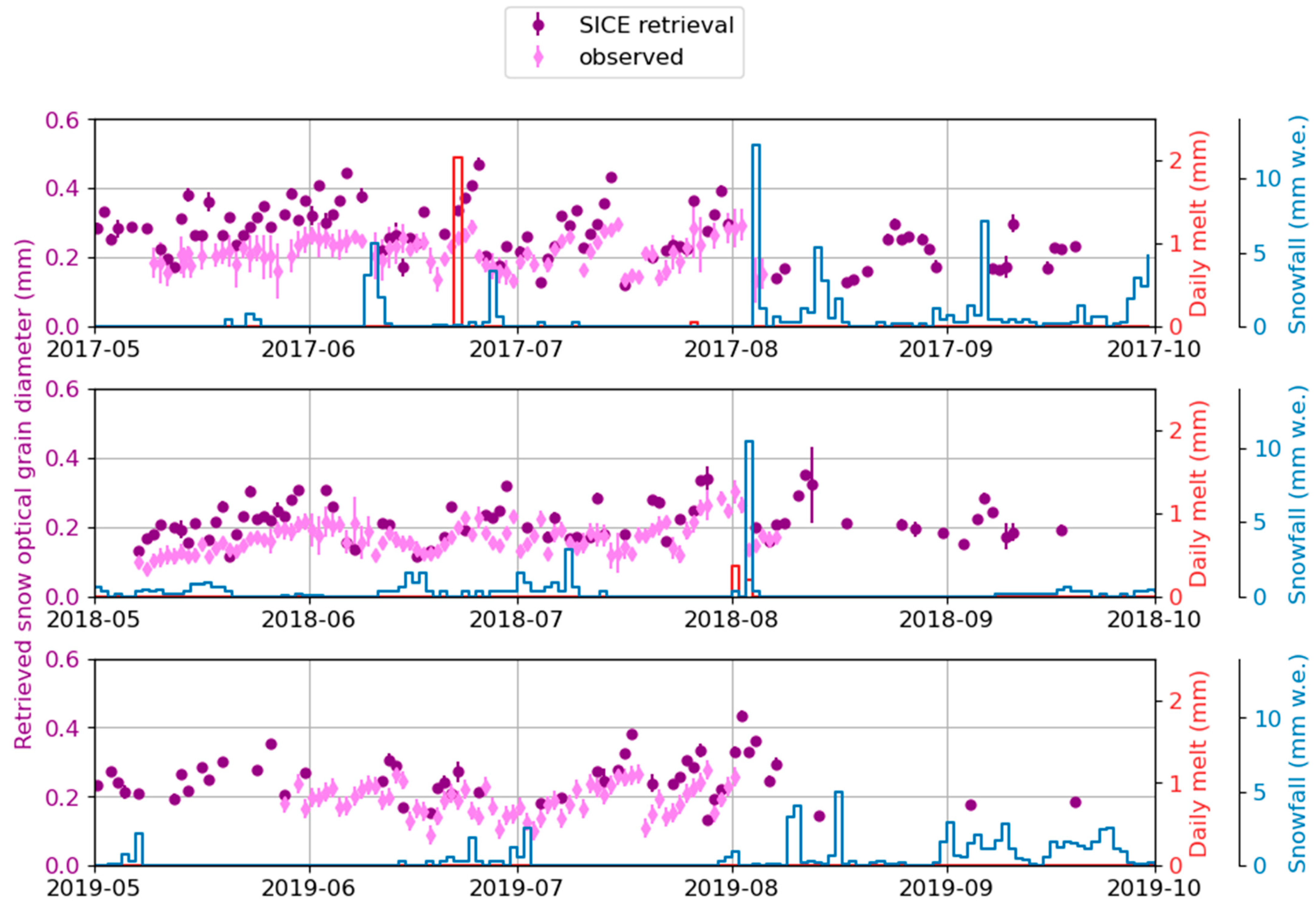
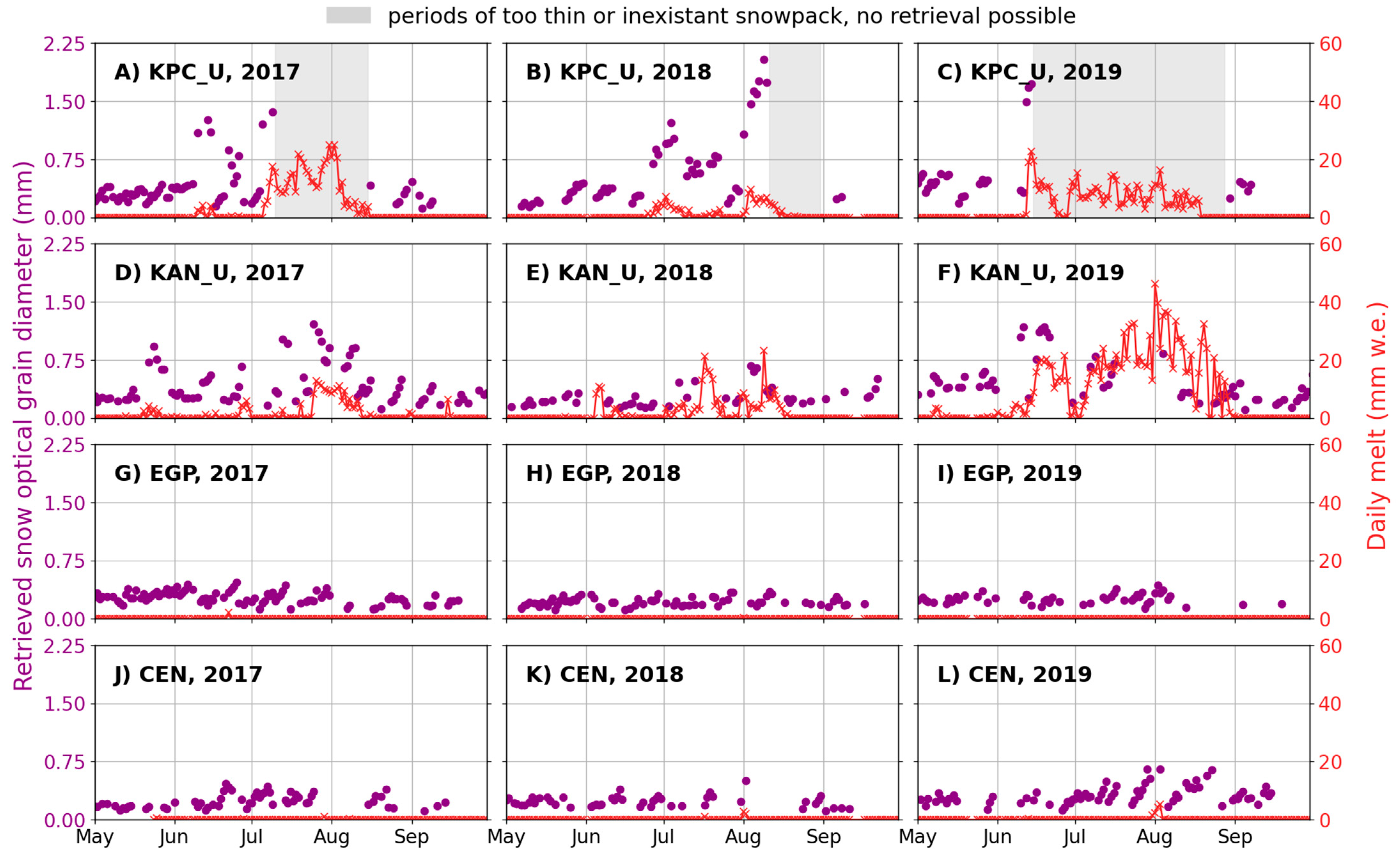
3.1. Evaluation of the Grain Size Rretrieval

The SICE retrievals of d o p t ranged from 0.10 to 0.47 mm while the measured d o p t derived from in situ SSA measurements at EGP ranged from 0.08 to 0.30 mm corresponding to SSA between 22 and 85 m2 kg−1 (Figure 1). The retrieved d o p t is on average 0.06 mm (30%) larger than the in situ measurements (Table 2, Figure 1). The daily standard deviation of measurements (error bars in Figure 1) relates to the spatial variability of d o p t along the 90 m transect and has an average of 0.03 mm. The spatial variability within the 90 m transect is therefore insufficient to explain the difference between the in situ measurements and retrieved d o p t . This difference could also be due to the deeper penetration of light within the snow at the 865 nm wavelength used for the SICE retrieval (down to ~3 cm, Figure 1 in [85]). The IceCube device uses a laser at a wavelength (1310 nm) corresponding to a sampling depth of less than 2 cm below the surface. In springtime, d o p t is minimal at the surface and increases with depth when snow grains have time to undergo metamorphism [29,86,87]. Consequently, a systematic difference of sampling depth in the SICE retrieval and IceCube measurement will lead to a systematic difference in the grain size they estimate. Measurements and retrievals show linear correlation with Pearson’s correlation (r) ranging from 0.50 to 0.62 depending on the year (Table 2).
A short and low intensity (2 mm w.e.) surface melt episode on 22 June 2017 is associated with an increase in both the ground observation and the satellite retrieval optical snow grain diameter (Figure 1). The ground observation and retrieved d o p t continued to increase for the 2–3 following days when melt was not calculated but warm temperatures continued to heat the surface. This melt event is small, with less than 2 mm w.e. for the full day. Such surface melt rates represent minor changes at the surface and limited generation of liquid water. Consequently, the d o p t increases on 22 June 2017 were only slightly more pronounced than other increases that occurred during periods when melt was not calculated at the weather station. Major snowfall events recorded by the AWS led to a decrease of grain size by a factor of two or more (Figure 1). In some occurrences (e.g., 18 July 2018), the d o p t decreased without the AWS recording any precipitation. A possible cause is wind transporting small grains to the site, as also hypothesized by [29]. However, no clear covariation of d o p t and wind speed measured at the AWS could be found at EastGRIP.

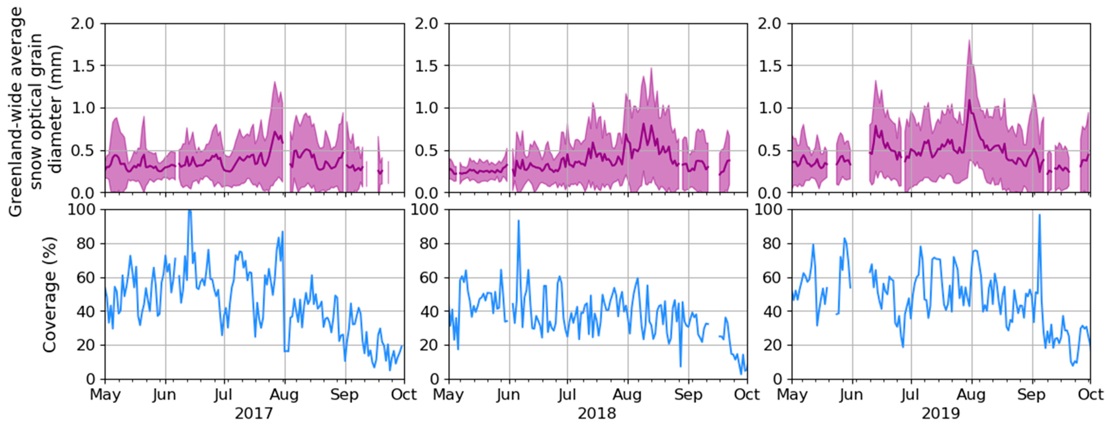
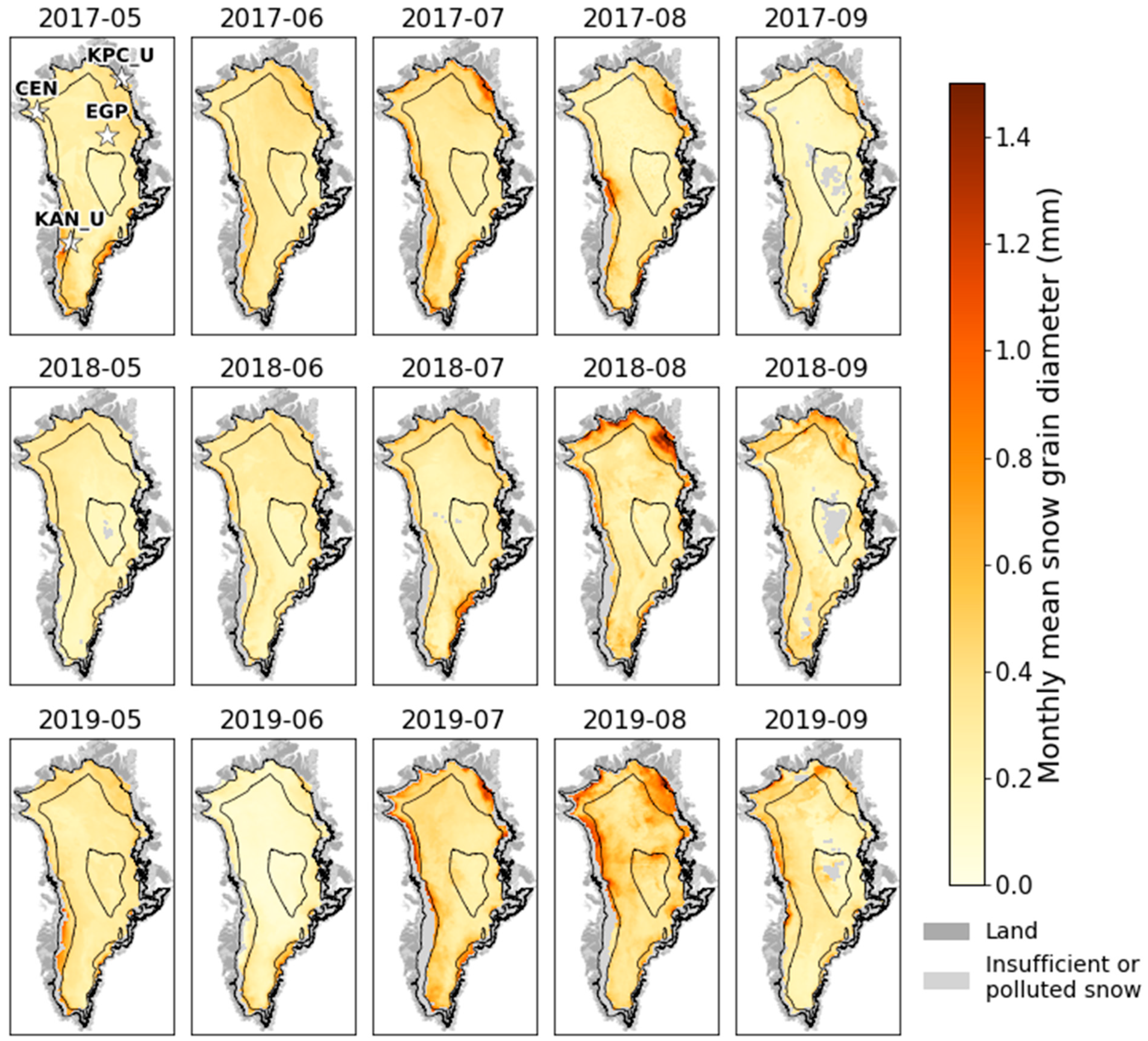
3.2. The SICE Snow Optical Grain Diameter Dataset

The SICE toolchain provides daily snapshots of optical snow grain diameter at a 1 km resolution. The main challenge for shortwave optical remote sensing is the impossibility of retrieval during cloudy conditions. The average cloud-free coverage was 45% in 2017, 31.8% in 2018 and 40% in 2019 (Figure 2). The ice-sheet-wide snow-covered area-only mean d o p t was around 0.3 mm at the beginning of the season and peaked above 0.6 mm around late July or early August, when surface melt is widespread. The smaller standard deviation in May indicates the relative homogeneity of cold, dry snow grains at the surface in the early melt season. As melt starts on the southern and low-lying ice sheet, the standard deviation increases and reaches its maximum synchronously with the average d o p t , at the peak of the melt season. The warm year of 2019, during which melt was well above average [88], also had the highest Greenland-wide average d o p t : 0.45 mm compared to 0.36 mm for both 2017 and 2018. That year (2019) also has the maximum daily mean value (1.08 mm on 31 July 2019; Figure 2), as compared to a respective maximum of 0.71 mm and 0.81 mm in 2017 and 2018.
During the melting season, the melt is triggered initially in southern and low-elevation areas before it spreads northward and to more-elevated areas. d o p t follows a similar evolution (Figure 3 and Supplementary Figure S1). At the beginning of the season, before the melt onset, the retrieved d o p t is relatively low and homogeneous across the ice sheet (e.g., low standard deviation of grain diameters in May 2018, Figure 2) and does not show a visible gradient with elevation (e.g., northern and western regions in Figure 3 and Supplementary Figure S1). Where and when surface warming and melting started, the lowermost areas saw an increase of d o p t and of its spatial heterogeneity (Figure 3 and Supplementary Figure S1), while higher areas still had a relatively low and homogeneous d o p t . In the southern areas and in warm years such as 2019, the grain diameter spatial gradients are visible already in May, when the first retrievals are available (e.g., southwestern regions in Figure 3). As the surface heating and melt progresses to higher elevations, the d o p t increase propagates to the ice sheet interior (Figure 3 and Supplementary Figure S1).

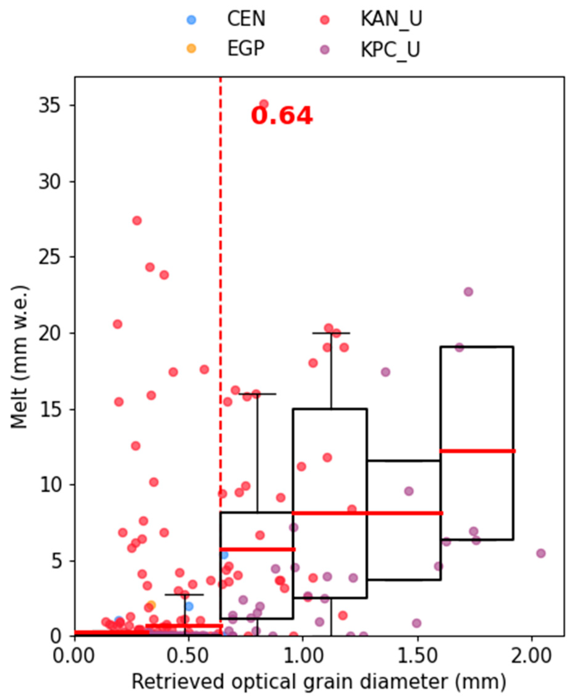
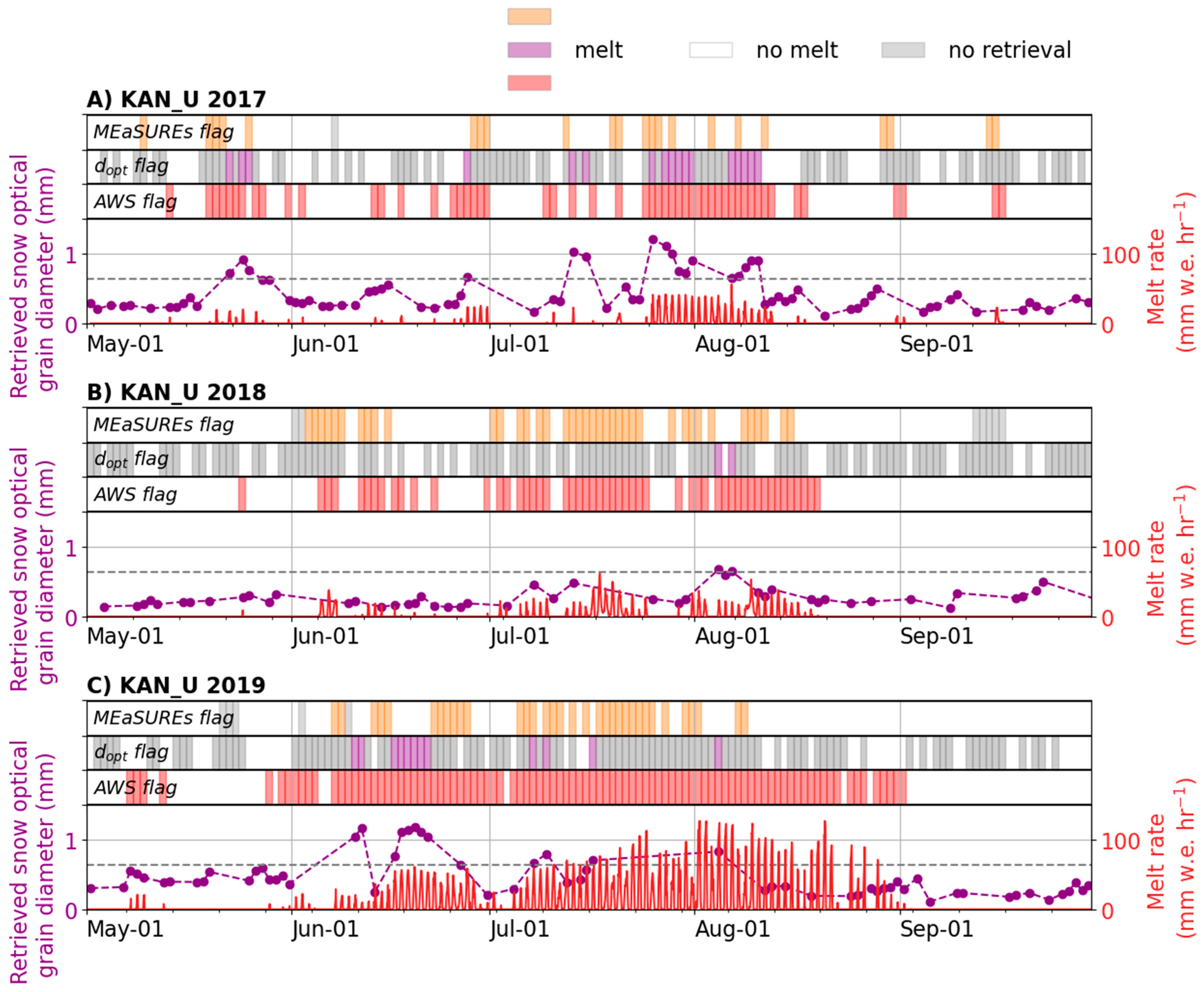
3.3. Optical Grain Diameter as an Indicator of Melt Affected Snow

At the four PROMICE AWS (Table 1), the calculated melt rates can be compared to the median d o p t retrieved within a 2 km radius of each AWS (Figure 4). The magnitude of melt calculated from the AWSs allows a better understanding of the covariation of d o p t and surface melt than at EastGRIP alone (Figure 1). The retrieved d o p t reacted closely to the presence and absence of surface melting. At most sites, the d o p t had values at or below 0.5 mm at the beginning of the season, when no melt was calculated. At melt onset, d o p t jumps above its premelt values at all sites (Figure 4). Some exceptions such as large d o p t in the absence of melt or small d o p t retrieved during the melt period can be noticed. These punctual decoupling of surface grain diameter and surface melt can be caused by errors in the retrieval, for instance due to cloud contamination or errors in the melt calculation due to inaccurate AWS measurements. A last potential explanation for mismatch cases is that the satellite retrieval may have been taken at an hour of the day when the surface was not melting, (Sentinel 3 overpass time is 10 am local time at nadir), but surface melt occurred later on that day.
The relation between the retrieved snow d o p t and the surface melt rate is complex. Pearson’s coefficient of correlation is 0.49, which reveals a co-variation of the two variables although a linear regression is incomplete in explaining the relationship. As an alternative, we look for the d o p t value that is most representative of melting conditions and so plot the calculated daily melt as a function of retrieved d o p t for our four sites over 2017–2019 (Figure 5). An analysis of variance indicates that a threshold of 0.64 mm in d o p t splits the samples into two coherent classes. The samples that have retrieved d o p t below 0.64 mm have a median melt of 0 mm w.e. and an average that is not significantly different from zero. The samples that have a retrieved d o p t > 0.64 mm have an average daily melt of 7.11 mm w.e., significantly greater than zero and greater than the average of the first class (p-value < 0.001, Figure 5). Additionally, 81.3% of the dopt retrieval above 0.64 mm corresponds to daily melt greater than 1 mm w.e. and 95.2% of the d o p t retrieval below or equal to 0.64 mm corresponds to daily melt lower than 1 mm w.e. This simple threshold approach classifies appropriately the majority of the days, either as melt days, when the retrieved d o p t is above that threshold, and non- or low-melt days when the retrieved d o p t is below that threshold. This stepwise approach nevertheless misclassifies 18.8% (12 out of 64) of samples as melt days when no or little melt was calculated those days. Similarly, 4.8% (32 out of 660) of days classified as non- or low-melt actually had more than 1 mm of melting calculated from the AWS data.
To assess the robustness of this threshold, we fitted similar stepwise functions to (i) each station-year (except CEN and EGP which did not present sufficient melt), (ii) all samples but removing each station iteratively and (iii) 2017, 2018 and 2019 separately (Supplementary Table S1). The thresholds found in these test cases have an average of 0.61 mm and a standard deviation of 0.10 mm, consistent with the threshold found when pooling all samples. However, the threshold found for these subsets are more sensitive to the errors that occur at each site arising from the difference of footprint between the satellite retrieval and the AWS measurements, erroneous measurements from the AWS that lead to improper melt calculation as well as cloud contamination that leads to improper d o p t estimation. We expect that by pooling all these measurements, random noise will be reduced, and a more robust threshold value can be found.

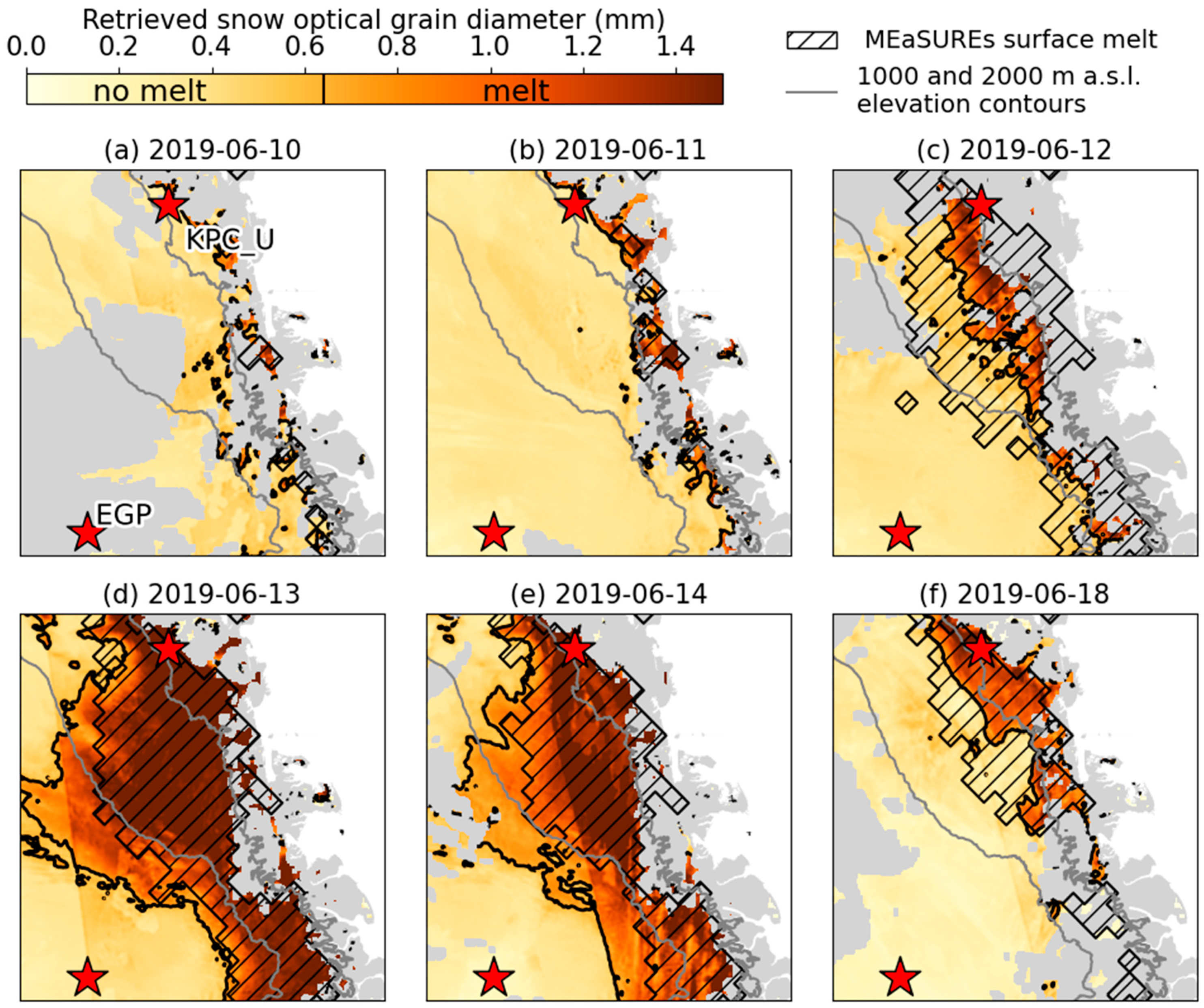
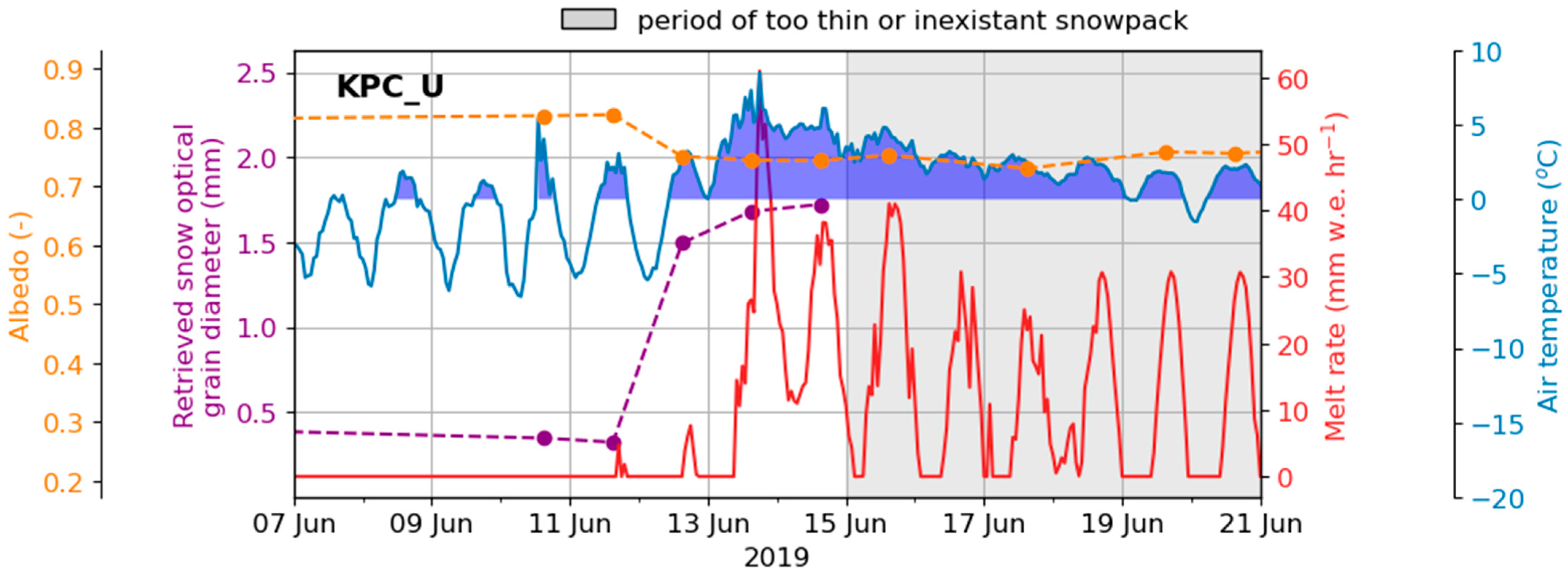
3.4. Application to a Heat Wave in Northeast Greenland and Comparison to the MEaSUREs Melt Flag

We now focus on the 10–18 July 2019 in Northeast Greenland (Figure 6), in the vicinity of the Northeast Greenland Ice Stream (NEGIS). In this area, warm air masses from the northern Atlantic are being pushed onto the Greenland ice sheet through the surface depression created by the NEGIS [90]. As an independent estimate of melting areas, the MEaSUREs melt flag, derived from passive microwave remote sensing, is also considered and compared to our d o p t -based melt flag.
On the 10th, the majority of the area shows relatively small d o p t . Only a narrow band below 650 m a.s.l. has a larger d o p t (Figure 6). KPC_L is located below that elevation and already showed a too thin snowpack by this point of the season and could not be used for this analysis. KPC_U is located at 870 m a.s.l. and was still snow-covered and untouched by melt as can be seen from the high albedo (~0.8) and the subfreezing air temperature measured before the start of the event (Figure 7). The MEaSUREs melt flag also indicates nonmelting conditions at KPC_U (Figure 6). On the 11th, both melt flags indicate nonmelting conditions at KPC_U. However, the AWS starts to detect minor melt for that day (Figure 7). This amount of melt is either below the detection limit of both melt flags or occurred during a narrow timespan and was missed by both satellites. On the 12th and the following days, the warming continues and the AWS, the d o p t -based flag and the MEaSUREs flag all indicate melt at KPC_U (Figure 6 and Figure 7). However, different spatial patterns can be seen in the two melt flags. On the 12th, MEaSUREs flag reaches altitudes up to 2000 m a.s.l. The d o p t -based flag shows a main melting area reaching up to 1600 m a.s.l. and isolated melting patches up to 1800 m a.s.l. On the 13th and 14th, it is in turn the d o p t -based melt flag that reaches the highest altitudes (up to 2400 m a.s.l.) while the MEaSUREs melting area does not reach higher than 2200 m a.s.l. (Figure 6). On the 18th, the melt stops at higher elevation and continues at below 1600 m a.s.l. According to the MEaSUREs flag and below 1200 m a.s.l. for the d o p t -based flag. During the entire period, the EGP AWS did not show any sign of melt either as calculated from the AWS data (Figure 1) or according to the two melt flags (Figure 6).
From this specific case, the SICE d o p t -based flag agrees with MEaSUREs melt flag on the overall spatial variation of the surface melting area. However, substantial differences between the two were highlighted. Unfortunately, no in situ melt data is available in the area where the two melt flags disagree. Additionally, the KPC_U AWS quickly loses its snowpack which limits the number of days for which both d o p t -based and MEaSUREs melt flags are available. At KAN_U however, melt is frequent, and the snow never melts out, making it an appropriate location to evaluate the two melt flags against the melt estimated from AWS data (Figure 8). As expected, there are more days where retrieval was impossible for the d o p t -based flag because of cloud cover: retrieval was possible for only 45% of days during May-September of 2017–2019. Considering the AWS-derived melt estimate as ground truth, accurate melt flagging, false positives and false negatives can be found for both melt flags (Figure 8, Table 3). The d o p t -based melt flag has a very low commission error, indicating very few false positives. The higher omission error indicate that some melt events are not flagged, but apart for 2018, omissions of the d o p t flag are comparable with the ones of MEaSUREs flag.

4. Discussion

To achieve a reasonable processing time and memory use, we resampled the OLCI images from ~350 m to a 1 km resolution. This spatial resolution is comparable to other snow optical grain diameter or SSA products [24,44]. When using the retrieved dopt to identify surface melt, the resulting 1 km resolution melt map represents a significant improvement compared to the 25 km resolution of surface melt maps produced from passive microwave data [12,53]. Recent efforts were made to enhance the resolution of the passive microwave observations [55]. Nevertheless, the in situ validation, at one AWS in [55], remained limited and the contamination of coarse passive microwave observations by land near the ice sheet margin remains problematic.
Our approach reveals spatially discontinuous and patchy melt areas (Figure 6). Nevertheless, even at the relatively fine 1 km resolution, melt may be spatially inhomogeneous within a pixel. This spatial heterogeneity complicates the comparison with pointwise AWS observations. Additionally, the nonmelting/melting binary flagging cannot represent the transformation of a melt-free pixel to a pixel where different snow patches can be melting at various intensities and finally to a fully melting pixel. Further, most of the PROMICE stations are located in lower ablation areas where the snowpack rapidly ablates and glacial ice is revealed, reducing the time over which spaceborne retrieval is relevant. CEN and EGP AWS are exceptional by being in the accumulation area and rarely seeing melt. Only two AWS, KPC_U and KAN_U, are located close to the equilibrium line and allow to assess the response of d o p t to surface melt. Future in situ estimation of surface melt, from AWS or other techniques, at the equilibrium line altitude could help to further document the relation between d o p t and either the presence or the intensity of surface melt.
The threshold that was found to identify melting conditions, d o p t = 0.64 mm, corresponds to an SSA of 0.11 m2 kg−1. It is consistent with previous values identified for melting surfaces such as 0.6 mm by [29] and ~0.5 mm in [24] (Figure 6 therein). Previous studies also used the optical characteristics of snow, such as albedo, as a proxy for melt and mass loss [91,92]. But such an approach only worked on annual averages. In our study, we have related daily changes in d o p t as a response to the presence or absence of meltwater at the surface estimated using the high-temporal-resolution AWS data.
In theory, it is possible that large melt-affected snow grains remain at the surface after the melt stops and consequently that our melt flag would show false positives after the end of the melt event. Although it is a plausible scenario, we do not see this occurring often in our dataset, potentially for two reasons. First, the pervasive action of wind on the ice sheet may quickly erode the surface layer. Small windblown snow grains then cover the melted snow and the d o p t -based flag is reset to nonmelting. Second, the end of the melt period coincides with cooler temperatures and consequently solid precipitation. The reflective fresh snow deposited at the surface has the potential to shut down the melt. In that situation, once the site becomes cloud-free again, our retrieval will identify fine grained fresh snow and nonmelting conditions. We note again that the presented flag only works for snow surfaces with low light-absorbing particle concentrations. More in situ observation will be needed to assess the performance of our d o p t retrieval for melting and non-melting polluted snow and to assess whether the same threshold on d o p t can be used to identify melt. Little is known about the optical properties of natural glacier ice surfaces, even less under melting conditions, and further research is needed to constrain radiative transfer models in those areas.
The penetration of solar radiation into surface snow implies that the SICE retrieval samples the first centimeters below the surface. The penetration depth also depends on the grain size [86] and shape [40] and on snow density. As a result, the thickness of the layer that is being sampled by our retrieval evolves throughout the season. Our retrieval assumes a vertically homogeneous snowpack, but since the near-surface snow grain size may vary vertically [21], multilayer snow models may be more suitable [38]. Nevertheless, multilayer radiative transfer models are computationally expensive and not convenient for near-real-time retrievals. Our retrieval also assumes a nonspherical grain shape (characterized by a shape factor B ( 1 g ) = 9.2 as in [50]). Although this assumption has been producing satisfactory results, it is far from the diversity of snow grain shapes in natural snowpacks [20,43,44]. Recent remote sensing efforts have included diverse grain shapes within the radiative transfer model [38,43,44]. Unfortunately, in situ measurements of grain shape at the relevant spatial scale for remote sensing product evaluation are not readily available to this day. In this absence of ground truth, the grain shape could only be used as a tuning parameter within radiative transfer models to minimize the difference between calculated and observed surface reflectances.
A recent report from the European Organisation for the Exploitation of Meteorological Satellites (EUMETSAT) evaluated the accuracy of the OLCI instruments onboard Sentinel-3A and B when measuring ocean reflectance [93]. They concluded that the OLCI measurements of surface reflectance at wavelength 865 nm were within the 2% accuracy defined in the mission requirements. However, the measured reflectances at 1020 nm were ~9% and ~6% too bright for Sentinel-3A and Sentinel-3B, respectively. These biases have been derived over dark ocean surfaces and cannot be used over bright snowy surfaces. No reference dataset is currently available for a vicarious calibration of OLCI over bright surfaces. The magnitude of this systematic bias should be subject of future research. However, since our melt detection threshold is chosen empirically, the melt maps derived here should remain unchanged by any future change of calibration, as the threshold could be accordingly re-evaluated.
When comparing our retrievals at 1 km resolution to in situ measurements, either for d o p t or for surface melt, the spatial representativity of these observations can be questioned. At EastGRIP, the surface type is relatively homogeneous, stemming from a smooth topography: the elevation does not vary by more than 7 m and the slope by more than 0.24° in the 1 km2 surrounding the station (derived from the GIMP DEM, [89]) suggesting uniform temperatures and incident shortwave radiation. At this site, the standard deviation of the d o p t along the 90 m observation transect, representative of the spatial heterogeneity, was 0.03 mm, which is significantly smaller than the difference between the observed and retrieved d o p t : 0.06 mm on average. Capturing the spatial heterogeneity in these dry snow regions is therefore less important than addressing the assumptions made in the retrieval procedure (e.g., grain shape or radiometric calibration). In the areas where surface melting is more prevalent, no in situ observation of d o p t , and of its spatial heterogeneity, is currently available for the Greenland ice sheet. Regarding the detection of surface melt, no observation currently allows bridging between point estimations at AWS sites and microwave melt flags at 12–25 km resolution [12,54]. We consequently compare point observations to gridded retrievals and let to future work bridging these scale gaps such as recently done for surface albedo measurements [94,95].

5. Conclusions

We presented the optical snow grain diameter ( d o p t ) retrieved for 3 years of Sentinel-3 OLCI observations over the Greenland ice sheet. After ensuring that the remotely sensed d o p t matches with in situ observations at EastGRIP, we analyzed the response of retrieved d o p t to surface warming and melt at four PROMICE automatic weather stations where melt can be calculated from meteorological measurements. We established that the retrieved d o p t and the in situ estimation of melt covary, which leads to a binary melt flag that can be constructed around the threshold d o p t of 0.64 mm with a high likelihood of melting above this threshold. We applied this threshold to our d o p t dataset and derived melt maps for daily 1 km mosaics of Greenland. We found that the spatiotemporal evolution of our melt flag compares well with the passive microwave MEaSUREs melt flag during a heat wave in Northeast Greenland and at the KAN_U PROMICE AWS. Although the two flags identify the same general periods and areas as melting, some spatial and temporal mismatches remain. For the dates when d o p t and the melt flag could be retrieved, it showed comparable accuracy (fraction of correct flags, 76%), omission (fraction of false negative, 51%) and commission (fraction of false positive, 1%) as the MEaSUREs melt flag (74%, 50% and 7% for the same metrics). Although our retrieval is not possible under cloud cover, which limits the coverage of the dataset, its 1 km spatial resolution is a great improvement compared to the MEaSUREs melt flag. d o p t can therefore be used at a regional scale or in combination with passive microwave to describe melt dynamics on the Greenland ice sheet at high spatial resolution.

Supplementary Materials

The following supporting information can be downloaded at: https://www.mdpi.com/article/10.3390/rs14040932/s1. Reference [96] is cited in the Supplementary Materials. Our Supplementary Figure S1 presents the retrieved optical snow grain diameter distribution on 1 June 2017 and 14 June 2017 for different elevation bins and in different drainage basins of the ice sheet.

Author Contributions

B.V. conceptualized the project, conducted the formal analysis, investigation and visualization. J.E.B. secured funding and administered the project and its resources. A.A.K. developed the retrieval methodology. B.V., J.E.B., A.W. and A.A.K. developed the retrieval software. A.W. curated data. M.H., A.-K.F., H.C.S.-L. and M.N. provided in situ data for retrieval validation. B.V., J.E.B., M.N. and G.P. drafted the original manuscript and all authors reviewed and edited the final manuscript. All authors have read and agreed to the published version of the manuscript.

Funding

This research was funded by the European Space Agency project “Scientific Exploitation of Operational Missions, Sentinel-3 Snow (Sentinel-3 for Science, Land Study 1: Snow)” (ESRIN contract No. 4000118926/16/I-NB, 2016–2019) EO Sci for Society (ESRIN contract No. 4000125043—ESA/AO/1-9101/17/I-NB, 2018–2020, and CCN 4000125043/18/I-NB, 2022–2023) and PRODEX, (2020–2022, technical officer: T. Ridder). Additional support came from the Program for the Monitoring of the Greenland Ice Sheet (PROMICE.dk), funded by the Danish Energy Agency through the DANCEA program. HCSL received funding from the European Research Council (ERC) under the European Union’s Horizon 2020 research and innovation program: Starting Grant-SNOWISO (grant agreement 759526).

Data Availability Statement

The daily mosaics of retrieved optical grain diameter, SSA and albedo are available at https://doi.org/10.22008/FK2/OIAJVO [97]. The scripts of the retrievals are available at https://doi.org/10.5281/zenodo.5179529 [57]. The PROMICE AWS data are available at https://doi.org/10.22008/promice/data/aws [78] and the scripts of the SEB model are available at https://doi.org/10.5281/zenodo.4542767 [98].

Acknowledgments

We thank Alexandra Zuhr, Sonja Wahl, Sepp Kipfstuhl and Melanie Behrens for their participation in the measurements of SSA at EastGRIP, Ken Mankoff for his contribution to the SICE project and our ESA technical officer Michael Kern.

Conflicts of Interest

The authors declare no conflict of interest.

References

  1. Flanner, M.G.; Shell, K.M.; Barlage, M.; Perovich, D.K.; Tschudi, M.A. Radiative forcing and albedo feedback from the Northern Hemisphere cryosphere between 1979 and 2008. Nat. Geosci. 2011, 4, 151–155. [Google Scholar] [CrossRef]
  2. Van Den Broeke, M.R.; Enderlin, E.M.; Howat, I.M.; Kuipers Munneke, P.; Noël, B.P.Y.; Jan Van De Berg, W.; Van Meijgaard, E.; Wouters, B. On the recent contribution of the Greenland ice sheet to sea level change. Cryosphere 2016, 10, 1933–1946. [Google Scholar] [CrossRef] [Green Version]
  3. Fettweis, X.; Box, J.E.; Agosta, C.; Amory, C.; Kittel, C.; Lang, C.; Van As, D.; Machguth, H.; Gallée, H. Reconstructions of the 1900–2015 Greenland ice sheet surface mass balance using the regional climate MAR model. Cryosphere 2017, 11, 1015–1033. [Google Scholar] [CrossRef] [Green Version]
  4. Noël, B.; van de Berg, W.J.; Lhermitte, S.; van den Broeke, M.R. Rapid ablation zone expansion amplifies north Greenland mass loss. Sci. Adv. 2019, 5, 2–11. [Google Scholar] [CrossRef] [PubMed] [Green Version]
  5. Ryan, J.C.; Smith, L.C.; As, D.V.; Cooley, S.W.; Cooper, M.G.; Pitcher, L.H.; Hubbard, A. Greenland Ice Sheet surface melt amplified by snowline migration and bare ice exposure. Sci. Adv. 2019, 5, eaav3738. [Google Scholar] [CrossRef] [Green Version]
  6. Wehrlé, A.; Box, J.E.; Niwano, M.; Anesio, A.M.; Fausto, R.S. Greenland bare-ice albedo from promice automatic weather station measurements and sentinel-3 satellite observations. Geol. Surv. Den. Greenl. Bull. 2021, 47. [Google Scholar] [CrossRef]
  7. Wang, W.; Zender, C.S.; van As, D.; Fausto, R.S.; Laffin, M.K. Greenland Surface Melt Dominated by Solar and Sensible Heating. Geophys. Res. Lett. 2021, 48, e2020GL090653. [Google Scholar] [CrossRef]
  8. Warren, S.G.; Wiscombe, W.J. A model for the spectral albedo of snow. II: Snow containing atmospheric aerosols. J. Atmos. Sci. 1980, 37, 2734–2745. [Google Scholar] [CrossRef]
  9. Wiscombe, W.J.; Warren, S.G. A model for the spectral albedo of snow. I: Pure snow. J. Atmos. Sci. 1980, 37, 2712–2733. [Google Scholar] [CrossRef] [Green Version]
  10. Gardner, A.S.; Sharp, M.J. A review of snow and ice albedo and the development of a new physically based broadband albedo parameterization. J. Geophys. Res. Earth Surf. 2010, 115, F01009. [Google Scholar] [CrossRef]
  11. Dumont, M.; Brun, E.; Picard, G.; Michou, M.; Libois, Q.; Petit, J.R.; Geyer, M.; Morin, S.; Josse, B. Contribution of light-absorbing impurities in snow to Greenland’s darkening since 2009. Nat. Geosci. 2014, 7, 509–512. [Google Scholar] [CrossRef]
  12. Mote, T.L. Greenland surface melt trends 1973–2007: Evidence of a large increase in 2007. Geophys. Res. Lett. 2007, 34, L22507. [Google Scholar] [CrossRef]
  13. Houtz, D.; Naderpour, R.; Schwank, M.; Steffen, K. Snow wetness and density retrieved from L-band satellite radiometer observations over a site in the West Greenland ablation zone. Remote Sens. Environ. 2019, 235, 111361. [Google Scholar] [CrossRef]
  14. Abdalati, W.; Steffen, K. Accumulation and hoar effects on microwave emission in the Greenland ice-sheet dry-snow zones. J. Glaciol. 1998, 44, 523–531. [Google Scholar] [CrossRef] [Green Version]
  15. Smith, B.E.; Gardner, A.; Schneider, A.; Flanner, M. Modeling biases in laser-altimetry measurements caused by scattering of green light in snow. Remote Sens. Environ. 2018, 215, 398–410. [Google Scholar] [CrossRef]
  16. Davis, C.H.; Zwally, H.J. Geographic and seasonal variations in the surface properties of the ice sheets by satellite-radar altimetry. J. Glaciol. 1993, 39, 687–697. [Google Scholar] [CrossRef] [Green Version]
  17. Larue, F.; Picard, G.; Aublanc, J.; Arnaud, L.; Robledano-Perez, A.; LE Meur, E.; Favier, V.; Jourdain, B.; Savarino, J.; Thibaut, P. Radar altimeter waveform simulations in Antarctica with the Snow Microwave Radiative Transfer Model (SMRT). Remote Sens. Environ. 2021, 263, 112534. [Google Scholar] [CrossRef]
  18. Verjans, V.; Leeson, A.A.; Max Stevens, C.; MacFerrin, M.; Noël, B.; Van Den Broeke, M.R. Development of physically based liquid water schemes for Greenland firn-densification models. Cryosphere 2019, 13, 1819–1842. [Google Scholar] [CrossRef] [Green Version]
  19. Fily, M.; Bourdelles, B.; Dedieu, J.P.; Sergent, C. Comparison of In situ and Landsat thematic mapper derive snow grain characteristics in the Alps. Remote Sens. Environ. 1997, 59, 452–460. [Google Scholar] [CrossRef]
  20. Fierz, C.; Armstrong, R.L.R.L.; Durand, Y.; Etchevers, P.; Greene, E.; McClung, D.M.D.M.; Nishimura, K.; Satyawali, P.K.; Sokratov, S.A. The International Classification for Seasonal Snow on the Ground. IHP-VII Tech. Doc. Hydrol. 2009, 83, 90. [Google Scholar]
  21. Aoki, T.; Hori, M.; Motoyoshi, H.; Tanikawa, T.; Hachikubo, A.; Sugiura, K.; Yasunari, T.J.; Storvold, R.; Eide, H.A.; Stamnes, K.; et al. ADEOS-II/GLI snow/ice products—Part II: Validation results using GLI and MODIS data. Remote Sens. Environ. 2007, 111, 274–290. [Google Scholar] [CrossRef]
  22. Grenfell, T.C.; Perovich, D.K.; Ogren, J.A. Spectral albedos of an alpine snowpack. Cold Reg. Sci. Technol. 1981, 4, 121–127. [Google Scholar] [CrossRef]
  23. Warren, S.G. Optical properties of snow. Rev. Geophys. 1982, 20, 67–89. [Google Scholar] [CrossRef]
  24. Lyapustin, A.; Tedesco, M.; Wang, Y.; Aoki, T.; Hori, M.; Kokhanovsky, A. Retrieval of snow grain size over Greenland from MODIS. Remote Sens. Environ. 2009, 113, 1976–1987. [Google Scholar] [CrossRef]
  25. Carlsen, T.; Birnbaum, G.; Ehrlich, A.; Freitag, J.; Heygster, G.; Istomina, L.; Kipfstuhl, S.; Orsi, A.; Schäfer, M.; Wendisch, M. Comparison of different methods to retrieve effective snow grain size in central Antarctica. Cryosphere Discuss. 2017, 6, 1–20. [Google Scholar] [CrossRef]
  26. Carmagnola, C.M.; Morin, S.; Lafaysse, M.; Domine, F.; Lesaffre, B.; Lejeune, Y.; Picard, G.; Arnaud, L. Implementation and evaluation of prognostic representations of the optical diameter of snow in the SURFEX/ISBA-Crocus detailed snowpack model. Cryosphere 2014, 8, 417–437. [Google Scholar] [CrossRef] [Green Version]
  27. Brun, E. Investigation on wet-snow metamorphism in respect of liquid-water content. Ann. Glaciol. 1989, 13, 22–26. [Google Scholar] [CrossRef] [Green Version]
  28. Domine, F.; Taillandier, A.S.; Cabanes, A.; Douglas, T.A.; Sturm, M. Three examples where the specific surface area of snow increased over time. Cryosphere 2009, 3, 31–39. [Google Scholar] [CrossRef] [Green Version]
  29. Xiong, C.; Shi, J. Snow specific surface area remote sensing retrieval using a microstructure based reflectance model. Remote Sens. Environ. 2018, 204, 838–849. [Google Scholar] [CrossRef]
  30. Mary, A.; Dumont, M.; Dedieu, J.-P.; Durand, Y.; Sirguey, P.; Milhem, H.; Mestre, O.; Negi, H.S.; Kokhanovsky, A.A.; Lafaysse, M.; et al. Intercomparison of retrieval algorithms for the specific surface area of snow from near-infrared satellite data in mountainous terrain, and comparison with the output of a semi-distributed snowpack model. Cryosphere 2013, 7, 741–761. [Google Scholar] [CrossRef] [Green Version]
  31. Dozier, J.; Schneider, S.R.; McGinnis, D.F. Effect of grain size and snowpack water equivalence on visible and near-infrared satellite observations of snow. Water Resour. Res. 1981, 17, 1213–1221. [Google Scholar] [CrossRef] [Green Version]
  32. Dozier, J. Spectral signature of alpine snow cover from the landsat thematic mapper. Remote Sens. Environ. 1989, 28, 9–22. [Google Scholar] [CrossRef]
  33. Bourdelles, B.; Fily, M. Snow grain-size determination from Landsat imagery over Terre Adelie, Antarctica. Ann. Glaciol. 1993, 17, 1723–1738. [Google Scholar] [CrossRef] [Green Version]
  34. Painter, T.H.; Rittger, K.; McKenzie, C.; Slaughter, P.; Davis, R.E.; Dozier, J. Retrieval of subpixel snow covered area, grain size, and albedo from MODIS. Remote Sens. Environ. 2009, 113, 868–879. [Google Scholar] [CrossRef] [Green Version]
  35. Stamnes, K.; Li, W.; Eide, H.; Aoki, T.; Hori, M.; Storvold, R. ADEOS-II/GLI snow/ice products—Part I: Scientific basis. Remote Sens. Environ. 2007, 111, 258–273. [Google Scholar] [CrossRef]
  36. Hori, M.; Aoki, T.; Stamnes, K.; Li, W. ADEOS-II/GLI snow/ice products—Part III: Retrieved results. Remote Sens. Environ. 2007, 111, 291–336. [Google Scholar] [CrossRef]
  37. Grenfell, T.C.; Warren, S.G. Representation of a nonspherical ice particle by a collection of independent spheres for scattering and absorption of radiation. J. Geophys. Res. Atmos. 1999, 104, 31697–31709. [Google Scholar] [CrossRef]
  38. Jin, Z.; Charlock, T.P.; Yang, P.; Xie, Y.; Miller, W. Snow optical properties for different particle shapes with application to snow grain size retrieval and MODIS/CERES radiance comparison over Antarctica. Remote Sens. Environ. 2008, 112, 3563–3581. [Google Scholar] [CrossRef]
  39. Zege, E.P.; Katsev, I.L.; Malinka, A.V.; Prikhach, A.S.; Heygster, G.; Wiebe, H. Algorithm for retrieval of the effective snow grain size and pollution amount from satellite measurements. Remote Sens. Environ. 2011, 115, 2674–2685. [Google Scholar] [CrossRef]
  40. Libois, Q.; Picard, G.; France, J.L.; Arnaud, L.; Dumont, M.; Carmagnola, C.M.; King, M.D. Influence of grain shape on light penetration in snow. Cryosphere 2013, 7, 1803–1818. [Google Scholar] [CrossRef] [Green Version]
  41. Yang, Y.; Marshak, A.; Han, M.; Palm, S.P.; Harding, D.J. Snow grain size retrieval over the polar ice sheets with the Ice, Cloud, and land Elevation Satellite (ICESat) observations. J. Quant. Spectrosc. Radiat. Transf. 2017, 188, 159–164. [Google Scholar] [CrossRef] [Green Version]
  42. Tanikawa, T.; Kuchiki, K.; Aoki, T.; Ishimoto, H.; Hachikubo, A.; Niwano, M.; Hosaka, M.; Matoba, S.; Kodama, Y.; Iwata, Y.; et al. Effects of Snow Grain Shape and Mixing State of Snow Impurity on Retrieval of Snow Physical Parameters from Ground-Based Optical Instrument. J. Geophys. Res. Atmos. 2020, 125, e2019JD031858. [Google Scholar] [CrossRef]
  43. Mei, L.; Rozanov, V.; Pohl, C.; Vountas, M.; Burrows, J.P. The retrieval of snow properties from SLSTR Sentinel-3-Part 1: Method description and sensitivity study. Cryosphere 2021, 15, 2757–2780. [Google Scholar] [CrossRef]
  44. Mei, L.; Rozanov, V.; Jäkel, E.; Cheng, X.; Vountas, M.; Burrows, J.P. The retrieval of snow properties from SLSTR Sentinel-3-Part 2: Results and validation. Cryosphere 2021, 15, 2781–2802. [Google Scholar] [CrossRef]
  45. Kokhanovsky, A. Snow Optics; Springer Nature: Cham, Switzerland, 2021. [Google Scholar]
  46. Tedesco, M.; Kokhanovsky, A.A. The semi-analytical snow retrieval algorithm and its application to MODIS data. Remote Sens. Environ. 2007, 111, 228–241. [Google Scholar] [CrossRef]
  47. Kokhanovsky, A.; Rozanov, V.V.; Aoki, T.; Odermatt, D.; Brockmann, C.; Krüger, O.; Bouvet, M.; Drusch, M.; Hori, M. Sizing snow grains using backscattered solar light. Int. J. Remote Sens. 2011, 32, 6975–7008. [Google Scholar] [CrossRef]
  48. Wiebe, H.; Heygster, G.; Zege, E.; Aoki, T.; Hori, M. Snow grain size retrieval SGSP from optical satellite data: Validation with ground measurements and detection of snow fall events. Remote Sens. Environ. 2013, 128, 11–20. [Google Scholar] [CrossRef]
  49. Kokhanovsky, A.; Schreier, M. The determination of snow specific surface area, albedo and effective grain size using AATSR space-borne measurements. Int. J. Remote Sens. 2009, 30, 919–933. [Google Scholar] [CrossRef]
  50. Kokhanovsky, A.; Lamare, M.; Danne, O.; Brockmann, C.; Dumont, M.; Picard, G.; Arnaud, L.; Favier, V.; Jourdain, B.; Meur, E.L.E.L.; et al. Retrieval of snow properties from the Sentinel-3 Ocean and Land Colour Instrument. Remote Sens. 2019, 11, 2280. [Google Scholar] [CrossRef] [Green Version]
  51. Kokhanovsky, A.; Box, J.E.; Vandecrux, B.; Mankoff, K.D.; Lamare, M.; Smirnov, A.; Kern, M. The determination of snow albedo from satellite measurements using fast atmospheric correction technique. Remote Sens. 2020, 12, 234. [Google Scholar] [CrossRef] [Green Version]
  52. Tedesco, M. Assessment and development of snowmelt retrieval algorithms over Antarctica from K-band spaceborne brightness temperature (1979–2008). Remote Sens. Environ. 2009, 113, 979–997. [Google Scholar] [CrossRef]
  53. Abdalati, W.; Steffen, K. Greenland ice sheet melt extent: 1979–1999. J. Geophys. Res. Atmos. 2001, 106, 33983–33988. [Google Scholar] [CrossRef]
  54. Fettweis, X.; Tedesco, M.; Van Den Broeke, M.; Ettema, J. Melting trends over the Greenland ice sheet (1958–2009) from spaceborne microwave data and regional climate models. Cryosphere 2011, 5, 359–375. [Google Scholar] [CrossRef] [Green Version]
  55. Colosio, P.; Tedesco, M.; Ranzi, R.; Fettweis, X. Surface melting over the Greenland ice sheet derived from enhanced resolution passive microwave brightness temperatures (1979–2019). Cryosphere 2021, 15, 2623–2646. [Google Scholar] [CrossRef]
  56. Long, D.G.; Daum, D.L. Spatial resolution enhancement of SSM/I data. IEEE Trans. Geosci. Remote Sens. 1998, 36, 407–417. [Google Scholar] [CrossRef] [Green Version]
  57. Vandecrux, B.; Mankoff, K.; Wehrlé, A.; Kokhanovsky, A.A.; Box, J.E. GEUS-SICE/SICE: SICE: Sentinel-3 Snow and Ice Properties Retrieval (2.0). Zenodo 2021. [Google Scholar] [CrossRef]
  58. ESA SENTINEL-3 OLCI User Guide. Available online: https://sentinel.esa.int/web/sentinel/user-guides/sentinel-3-olci (accessed on 3 January 2022).
  59. Copernicus Sentinel Data. Available online: https://www.esa.int/Applications/Observing_the_Earth/Copernicus (accessed on 3 January 2022).
  60. SNAP. Available online: http://step.esa.int (accessed on 3 January 2022).
  61. Thuillier, G.; Hersé, M.; Labs, D.; Foujols, T.; Peetermans, W.; Gillotay, D.; Simon, P.C.; Mandel, H. The solar spectral irradiance from 200 to 2400 nm as measured by the SOLSPEC spectrometer from the ATLAS and EURECA missions. Sol. Phys. 2003, 214, 1–22. [Google Scholar] [CrossRef]
  62. Lamquin, N.; Clerc, S.; Bourg, L.; Donlon, C. OLCI A/B Tandem Phase Analysis, Part 1: Level 1 Homogenisation and Harmonisation. Remote Sens. 2020, 12, 1804. [Google Scholar] [CrossRef]
  63. Sentinel-3 OLCI Level-0 and Level-1B ATBD. Available online: https://sentinel.esa.int/documents/247904/2702575/Sentinel-3-OLCI-Level-0-and-1B-ATBD.pdf (accessed on 3 January 2022).
  64. Metsämäki, S.; Pulliainen, J.; Salminen, M.; Luojus, K.; Wiesmann, A.; Solberg, R.; Böttcher, K.; Hiltunen, M.; Ripper, E. Introduction to GlobSnow Snow Extent products with considerations for accuracy assessment. Remote Sens. Environ. 2015, 156, 96–108. [Google Scholar] [CrossRef]
  65. Wehrlé, A.; Box, J. SICE implementation of the Simple Cloud Detection Algorithm (SCDA) v2.0. GEUS Dataverse V1 2021. [Google Scholar] [CrossRef]
  66. Sentinel-3 Product Notice—SLSTR. Available online: https://www.eumetsat.int/media/42788 (accessed on 3 January 2022).
  67. Kokhanovsky, A.; Lamare, M.; Di Mauro, B.; Picard, G.; Arnaud, L.; Dumont, M.; Tuzet, F.; Brockmann, C.; Box, J.E. On the reflectance spectroscopy of snow. Cryosphere 2018, 12, 2371–2382. [Google Scholar] [CrossRef] [Green Version]
  68. Zege, E.P.; Kokhanovsky, A.A. Analytical solution to the optical transfer function of a scattering medium with large particles. Appl. Opt. 1994, 33, 6547. [Google Scholar] [CrossRef] [PubMed]
  69. Kokhanovsky, A.A.; Zege, E.P. Scattering optics of snow. Appl. Opt. 2004, 43, 1589. [Google Scholar] [CrossRef]
  70. Zege, E.P.; Ivanov, A.; Katsev, I. Image Transfer through a Scattering Medium; Springer: Berlin, Germany, 1991. [Google Scholar]
  71. Sobolev, V.V. Light Scattering in Planetary Atmospheres; Pergamon Press: Oxford, UK, 1975; ISBN 9781483187280. [Google Scholar]
  72. Warren, S.G.; Brandt, R.E. Optical constants of ice from the ultraviolet to the microwave: A revised compilation. J. Geophys. Res. Atmos. 2008, 113, D14220. [Google Scholar] [CrossRef]
  73. Kokhanovsky, A.A.; Macke, A. Integral light-scattering and absorption characteristics of large, nonspherical particles. Appl. Opt. 1997, 36, 8785. [Google Scholar] [CrossRef] [PubMed]
  74. Kokhanovsky, A.A. Scaling constant and its determination from simultaneous measurements of light reflection and methane adsorption by snow samples. Opt. Lett. 2006, 31, 3282. [Google Scholar] [CrossRef]
  75. Domine, F.; Salvatori, R.; Legagneux, L.; Salzano, R.; Fily, M.; Casacchia, R. Correlation between the specific surface area and the short wave infrared (SWIR) reflectance of snow. Cold Reg. Sci. Technol. 2006, 46, 60–68. [Google Scholar] [CrossRef]
  76. Madsen, M.V.; Steen-Larsen, H.C.; Hörhold, M.; Box, J.; Berben, S.M.P.; Capron, E.; Faber, A.-K.; Hubbard, A.; Jensen, M.F.; Jones, T.R.; et al. Evidence of Isotopic Fractionation During Vapor Exchange Between the Atmosphere and the Snow Surface in Greenland. J. Geophys. Res. Atmos. 2019, 124, 2932–2945. [Google Scholar] [CrossRef] [Green Version]
  77. Gallet, J.C.; Domine, F.; Zender, C.S.; Picard, G. Measurement of the specific surface area of snow using infrared reflectance in an integrating sphere at 1310 and 1550 nm. Cryosphere 2009, 3, 167–182. [Google Scholar] [CrossRef] [Green Version]
  78. Fausto, R.S.R.S.; van As, D. Programme for monitoring of the Greenland ice sheet (PROMICE): Automatic weather station data. Version: v03. Geol. Surv. Den. Greenl. 2019. [Google Scholar] [CrossRef]
  79. Vandecrux, B.; Fausto, R.S.; Van As, D.; Colgan, W.; Langen, P.L.; Haubner, K.; Ingeman-Nielsen, T.; Heilig, A.; Stevens, C.M.; MacFerrin, M.; et al. Firn cold content evolution at nine sites on the Greenland ice sheet between 1998 and 2017. J. Glaciol. 2020, 66, 591–602. [Google Scholar] [CrossRef]
  80. Vandecrux, B.; Fausto, R.S.; Langen, P.L.; van As, D.; MacFerrin, M.; Colgan, W.T.; Ingeman-Nielsen, T.; Steffen, K.; Jensen, N.S.; Møller, M.T.; et al. Drivers of Firn Density on the Greenland Ice Sheet Revealed by Weather Station Observations and Modeling. J. Geophys. Res. Earth Surf. 2018, 123, 2563–2576. [Google Scholar] [CrossRef]
  81. Van As, D.; van den Broeke, M.; Reijmer, C.; van de Wal, R. The summer surface energy balance of the high Antarctic plateau. Boundary-Layer Meteorol. 2005, 115, 289–317. [Google Scholar] [CrossRef]
  82. Vandecrux, B.; Mottram, R.; Langen, P.L.; Fausto, R.S.; Olesen, M.; Stevens, M.; Verjans, V.; Leeson, A.; Ligtenberg, S.; Munneke, P.K.; et al. The firn meltwater Retention Model Intercomparison Project (RetMIP): Evaluation of nine firn models at four weather station sites on the Greenland ice sheet. Cryosphere 2020, 14, 3785–3810. [Google Scholar] [CrossRef]
  83. Mote, T.L. MEaSUREs Greenland Surface Melt Daily 25 km EASE-Grid 2.0, Version 1; NASA National Snow and Ice Data Center Distributed Active Archive Center: Boulder, CO, USA, 2014. [CrossRef]
  84. Meier, W.N.; Stewart, J.S. Assessment of the Stability of Passive Microwave Brightness Temperatures for NASA Team Sea Ice Concentration Retrievals. Remote Sens. 2020, 12, 2197. [Google Scholar] [CrossRef]
  85. Picard, G.; Libois, Q.; Arnaud, L.; Verin, G.; Dumont, M. Development and calibration of an automatic spectral albedometer to estimate near-surface snow SSA time series. Cryosphere 2016, 10, 1297–1316. [Google Scholar] [CrossRef] [Green Version]
  86. Li, W.; Stamnes, K.; Chen, B.; Xiong, X. Snow grain size retrieved from near-infrared radiances at multiple wavelengths. Geophys. Res. Lett. 2001, 28, 1699–1702. [Google Scholar] [CrossRef]
  87. Matoba, S.; Niwano, M.; Tanikawa, T.; Iizuka, Y.; Yamasaki, T.; Kurosaki, Y.; Aoki, T.; Hashimoto, A.; Hosaka, M.; Sugiyama, S. Field activities at the SIGMA-A site, northwestern Greenland Ice Sheet, 2017. Bull. Glaciol. Res. 2018, 36, 15–22. [Google Scholar] [CrossRef]
  88. Tedesco, M.; Fettweis, X. Unprecedented atmospheric conditions (1948–2019) drive the 2019 exceptional melting season over the Greenland ice sheet. Cryosphere 2020, 14, 1209–1223. [Google Scholar] [CrossRef] [Green Version]
  89. Howat, I.M.; Negrete, A.; Smith, B.E. The Greenland Ice Mapping Project (GIMP) land classification and surface elevation data sets. Cryosphere 2014, 8, 1509–1518. [Google Scholar] [CrossRef] [Green Version]
  90. Turton, J.V.; Mölg, T.; Van As, D. Atmospheric processes and climatological characteristics of the 79N glacier (Northeast Greenland). Mon. Weather Rev. 2019, 147, 1375–1394. [Google Scholar] [CrossRef]
  91. Colgan, W.; Box, J.E.; Fausto, R.S.; van As, D.; Barletta, V.R.; Forsberg, R. Surface albedo as a proxy for the mass balance of Greenland’s terrestrial ice. Geol. Surv. Denmark Greenl. Bull. 2014, 31, 91–94. [Google Scholar] [CrossRef] [Green Version]
  92. Davaze, L.; Rabatel, A.; Arnaud, Y.; Sirguey, P.; Six, D.; Letreguilly, A.; Dumont, M. Monitoring glacier albedo as a proxy to derive summer and annual surface mass balances from optical remote-sensing data. Cryosphere 2018, 12, 271–286. [Google Scholar] [CrossRef] [Green Version]
  93. Mazeran, C.; Ruescas, A. Ocean colour system vicarious calibration tool: Tool documentation (DOC-TOOL). EUMETSAT 2020. Report EUM/19/SVCT/D2. Available online: https://www.eumetsat.int/media/47502 (accessed on 3 January 2022).
  94. Ryan, J.C.; Hubbard, A.; Irvine-Fynn, T.D.; Doyle, S.H.; Cook, J.M.; Stibal, M.; Box, J.E. How robust are in situ observations for validating satellite-derived albedo over the dark zone of the Greenland Ice Sheet? Geophys. Res. Lett. 2017, 44, 6218–6225. [Google Scholar] [CrossRef] [Green Version]
  95. Irvine-fynn, T.D.L.; Bunting, P.; Cook, J.M.; Hubbard, A.; Barrand, N.E.; Hanna, E.; Hardy, A.J.; Hodson, A.J.; Holt, T.O.; Huss, M. Temporal Variability of Surface Reflectance Supersedes Spatial Resolution in Defining Greenland’s Bare-Ice Albedo. Remote Sens. 2022, 14, 62. [Google Scholar] [CrossRef]
  96. Zwally; Jay, H.; Giovinetto, M.B.; Beckley, M.A.; Saba, J.L. Antarctic and Greenland Drainage Systems, GSFC Cryospheric Sciences Laboratory. 2012. Available online: http://icesat4.gsfc.nasa.gov/cryo_data/ant_grn_drainage_systems.php (accessed on 3 January 2022).
  97. Vandecrux, B.; Box, J.; Mankoff, K.; Wehrlé, A. Snow broadband albedo, specific surface area and optical grain diameter from Sentinel-3’s OLCI, daily 1 km mosaics, Greenland. GEUS Dataverse V1 2021. [Google Scholar] [CrossRef]
  98. Vandecrux, B. BaptisteVandecrux/SEB_Firn_model: GEUS surface energy balance and firn model v0.3 (v0.3). Zenodo 2021. [Google Scholar] [CrossRef]
Figure 1. Observed and retrieved snow optical grain diameter ( d o p t ) at EastGRIP during May–October 2017–2019. Error bars indicate the daily standard deviation along the 90 m transect for observation and within a 2 km radius for the retrieval. Sonic ranger-derived snowfall and melt rate calculated from the PROMICE EGP AWS data.
Remotesensing 14 00932 g001
Figure 2. Greenland-wide average snow optical grain diameter ( d o p t ), ±1 standard deviation, and retrieval coverage as percent of Greenland ice sheet pixels for which retrieval was possible.
Remotesensing 14 00932 g002
Figure 3. Monthly average of retrieved snow optical grain diameter (dopt). Black lines indicate 1000 m elevation contours [89].
Remotesensing 14 00932 g003
Figure 4. Retrieved snow optical grain diameter (dopt, purple dots) and melt (red line and crosses) calculated from PROMICE AWS measurements.
Remotesensing 14 00932 g004
Figure 5. Daily melt calculated at the PROMICE AWSs and the retrieved snow optical grain diameter. Boxplots present statistics for 0.32 mm wide bins of optical grain diameter. The optical grain diameter threshold for melt detection is the dashed red line. In each boxplot, the whiskers represent the 5th and 95th percentiles, the edge of the box the 25th and 75th percentile and the solid red line represents the mean.
Remotesensing 14 00932 g005
Figure 6. Optical snow grain diameter retrieval and associated surface melt flag (areas within the black line) and MEaSUREs melt flag for a 10–18 June 2019 heat wave in Northeast Greenland along with AWS locations (red stars) and elevation contours (gray lines, 1000 and 2000 m a.s.l.).
Remotesensing 14 00932 g006
Figure 7. Retrieved snow grain optical diameter, plane broadband albedo, melt and air temperature at KPC_U AWS during the Northeast Greenland heat wave of June 2019.
Remotesensing 14 00932 g007
Figure 8. Comparison of three melt flags at KAN_U: (i) from MEaSUREs dataset; (ii) derived from a 0.64 mm threshold on the retrieved snow optical grain diameter ( d o p t ); and (iii) derived from the energy budget at the KAN_U AWS. The melting/nonmelting binary flag is shown in the upper part of each panel while retrieved snow optical grain diameter (purple dots), its 0.64 mm threshold value (dashed gray line) and the hourly AWS-derived melt (red line) are shown in the lower part of each panel.
Remotesensing 14 00932 g008
Table 1. Automatic weather station used for the investigation of surface melt.
StationLatitude (deg. N)Longitude (deg. E)Elevation (m a.s.l.)
KAN_U67.0003−47.02431840
KPC_U79.8345−25.1665870
EGP75.6247−35.97482700
CEN77.1826−61.11271886
Table 2. Comparison statistics between the measured and retrieved snow optical grain diameter at EastGRIP: Mean difference (MD), Root Mean Squared Difference (RMSD), Pearson’s correlation coefficient (r) and number of days used for comparison (N).
YearMD (mm)RMSD (mm)rN
all0.060.170.68145
20170.070.200.6259
20180.050.140.5957
20190.050.160.5029
Table 3. Comparison statistics of dopt-based and MEaSUREs melt flags. AWS-derived daily melt greater than 1 mm w.e. is taken as ground reference. The coverage is the fraction of days between 1st May and 30th of September for which a flag value is available. The accuracy is the fraction of days correctly classified by a flag. The omission error is the fraction of true melt days not detected by a flag. The commission error is the fraction of nonmelt days classified as melt by a flag.
MEaSUREs Melt Flag d o p t Melt Flag
YearCoverage (%)Accuracy (%)Omission Error (%)Commission Error (%)Coverage (%)Accuracy (%)Omission Error (%)Commission Error (%)
201799.277.765.66.751.690.527.82.2
201894.382.626.812.231.176.381.80
201998.463.356.4052.560.953.20
All97.374.450.37.345.175.851.31.1
Publisher’s Note: MDPI stays neutral with regard to jurisdictional claims in published maps and institutional affiliations.

