1. Introduction
Due to mass production and increasing affordability, the use of unmanned aerial vehicles (UAV) for forest monitoring is no longer the prerogative of advanced scientific teams. A similar trend has been observed in the software used for processing the data acquired by UAVs into 3D point clouds representing forest trees during laser scanning (light detection and ranging-Lidar) operations or its surface in the case of photogrammetry. Still, subsequent steps are necessary for extracting relevant information from forest point clouds, which tends to be quite fragmented, and it often requires intensive fitting for differing situations.
The detection of individual tree tops from UAV-based photogrammetry point clouds is a frequently discussed procedure, and different methods have been reviewed by several authors, for example [
1]. The local maximum filter (LMF) is one of the most commonly used methods. Several studies suggest that using LMF with a variable window size produces more promising results, especially in more diverse conditions [
2]. Nevertheless, the correct size of the window, whether fixed or variable, is critical for the results, and an incorrect size can lead to serious errors. Determining the window size is often a trial-and-error process for particular stands or situations. The R-project [
3] LidR package [
4] allows for a variable LMF window size based on the chosen function of the Z-coordinate of the point clouds in which the tree tops are identified. The tree crown width might serve as a good parameter for setting the window size based on the tree height [
2]. Using this method, a model is built using tree height to predict the crown diameter.
Several studies have concluded that the correlation between crown diameter and tree height is rather low; therefore, crown diameter prediction models are usually built using the tree stem diameter and several other independent variables [
5,
6,
7]. Because these variables are not available in our particular case, a linear mixed-effects model with NFI plots treated as a random effect was used. The local calibration [
8,
9] of this model was expected to provide an ideal means of establishing an appropriate LMF variable window size for a given area of interest. The Czechia National Forest Inventory (NFI) [
10] data provide a great opportunity to build such a model at the country level. Unmanned aerial laser scanning (ULS) point clouds together with the field survey results of tree counts on sample plots represent a promising means to assess the performance of local calibration based on different numbers of samples.
Although other individual tree detection methods that use, for example, info on the internal forest structure derived from ULS or airborne laser scanning (ALS) point clouds have started to emerge more recently [
11,
12], LMF represents one of the most common methods, especially for photogrammetry point clouds that are limited to the forest surface and that lack information on the internal structure. As stated above, using the correct window size in LMF applications is crucial for results. This study tries to confirm, whether local calibrated prediction of crown width might serve as a viable universal approach that can be used to determine the correct window size.
2. Materials and Methods
2.1. Study Site
Our study site, Skorkov (Lat: 50.2143906N, Lon: 14.7160739E; Position WGS 84), which is northeast of Prague, was established in a mixed forest stand comprising mostly flat terrain (188–190 m AMSL) and a species composition dominated by Pinus silvestris L. and Quercus robur L. Different age classes were present in 9.31 ha in rather rectangular arrangements, which is typical for Pinus management in this region.
2.2. Data Acquisition
The ULS point clouds were acquired using the UAV VUX-SYS setup (RIEGL Laser Measurement System GmbH, Horn, Austria) for UAV-borne data acquisition, which consisted of the UAV RiCOPTER, the VUX-1UAV laser scanner, and the AP-20 inertial measurement unit [
13]. The laser scanner was set to its maximum pulse frequency of 550 kHz and had a registration of 200 scanning lines per second. The flight was performed at a constant altitude of 90 m aboveground at a constant ground speed of 6 m·s
−1. This setup reached an average point density of 200 points·m
−2 for each scanning line. Due to the overlap between the individual scanning lines, the final mean point density was around 600 points·m
−2. All UAV flights complied with the national requirements stated in [
14] that were valid at the time of flight (September 2020), namely a maximum flight height below 300 m, a visual line of sight, airspace restrictions, and a minimal distance from people and buildings.
2.3. Laser Point Cloud Generation
The ULS point cloud was prepared from the data acquired by an UAV Ricopter equipped with a Riegl VUX-SYS1 sensor. The smoothed best trajectory estimates, which were based on the reference station post-processing kinematics with the virtual base station from Trimble VRS Now (Trimble Inc., Sunnyvale, CA, USA), were used and were prepared in the RiPROCESS environment using the RiPRECISSION module [
13]. Point cloud classification (for ground and non-ground points) was conducted in the same software environment.
2.4. Sample Plot Surveys
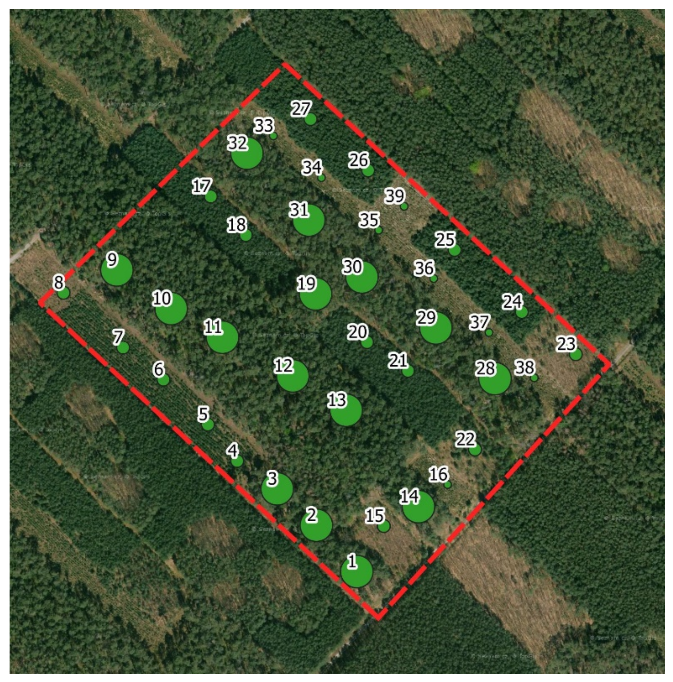
To gather relevant data to evaluate individual tree identification using an LMF procedure, a field survey was conducted. A total of 39 circular plots were established
Figure 1, with a variable plot radius related to the average tree height within the main canopy, which is shown in
Table 1.
On each sample plot, all of the trees over the minimal register limit were counted. A randomly chosen tree was also sampled for its height and crown parameters. In the class 1 plots, maximum and minimum crown projection diameters were measured by tape, and crown width was calculated as an average of these two measurements. For the class 2 and 3 plots, a procedure similar to the one used during NFI surveys [
10] was used, including measuring the position of the ground projection of at least five points defining the crown extent. The field survey was conducted using the Field-Map software/hardware set (IFER—Monitoring and Mapping Solutions Ltd., Jílové u Prahy, Czechia), which combines a flexible GIS software Field-Map with electronic equipment (Mapstar compass and ForestPro range-finder with inclinometer) for mapping and dendrometric measurements.
2.5. Crown Width Model Data
The NFI data acquired by the Forest Management Institute since 2001 were used to build linear mixed-effects models for the tree crown width predictions of individual trees based on height. The intended use of the model within the LMF procedure was limited to a single predictor variable, height; thus, other frequently employed variables [
5,
6,
7], such as diameter at breast height (DBH), were not employed to construct the crown prediction models. The NFI dataset included data on more than ninety-four thousand trees measured on more than twenty-two thousand plots, as seen in
Table 2. Only trees from the upper tree layer, which was determined as defined by the International Union of Forest Research Organizations and according to observed crown projection area and height measurements, were selected. The NFI field surveys [
10] identified tree crowns in the form of a horizontal projection area. For the purposes of this study, the crown width was calculated as a function of crown area by assuming a circular shape centered on the tree stem.
2.6. Model
A simple linear mixed-effects model was built iteratively with different predictor or predicted variable transformations to achieve optimal results. The best performing model was:
where
CWki is the crown width of tree
i in the stand/plot
k (m),
Hki is the height of tree
i in the stand/plot
k (m),
β0 and
β1 are fixed population parameters to be estimated,
α0k and
α1k are the random parameters to be estimated with zero expectations for stand
k, and
eki is the random residual error for tree
i on stand/plot
k. The
Hki variable had to be scaled, or else the model would not converge. This model is basically the same as the one described by Lappi [
8], which used height-DBH data.
The model parameters were first estimated using all of the trees from the NFI dataset with crown width and height measurements (n = 94,066), regardless of species, and the NFI plots were treated as a random parameter. This model was called f1. The model was developed in this manner in an effort to account for parameters other than height, as represented all together by individual inventory plot.
Based on the field surveys of the study site, a limited number of tree species are present, with three species representing the majority—P. sylvestris, Q. robur, and Quercus rubra L. Therefore, it was decided to create a subset of the NFI dataset to limit it to only the P. sylvestris and Quercus species, and this subset was then used to construct model f2.
2.7. Model Calibration
The use of a linear mixed-effects model allows for calibration within particular stands. Based on the sample data of crown widths and tree heights obtained at the stand of interest, the values of random parameters from equation Equation (1) can be estimated [
9] according to Equation (2).
where
is the matrix of estimated random parameters;
Z is the design matrix associated with random parameters;
is an estimate of
the variance–covariance matrix for the random parameters;
is the estimated variance–covariance matrix for residual errors of individual trees where
is the square of the residual standard error;
is a vector of predicted values from the fixed effect model; and
y is a vector of observations of the dependent variable from the particular stand.
To evaluate this calibration method on our model, one random plot from the NFI dataset was iteratively taken out as a calibration plot. The LME model (Equation (1)) was fitted to the NFI dataset without the calibration plot. Calibration was performed repeatedly based on the height and crown width data of 1, 3, 5, and 10 random trees from the calibration plot according to Equation (2).
The crown width was then estimated based on both the marginal model (without random parameters) and the calibrated model with estimated random parameters. Both estimates were compared to field-measured crown width values from the calibration plot using the normalized root mean squared error (
nRMSE; Equation (3)). This procedure was repeated one hundred times to assess the performance of the calibrated models.
where
n is the number of observations,
y is the observed value,
is mean of observed values, and
is the estimated value.
2.8. Study Site Calibration
For calibration of global models explained in the previous section, data that were obtained for the crown widths and heights in sample plots were used. A total of 39 trees were measured for this calibration. To evaluate the influence of the different number of calibration measurements both models were calibrated with randomly chosen 3, 5, 10, and all 39 calibration samples. Together with the uncalibrated marginal models, a total of 10 formulas were prepared for use during the LMF procedure. Model function names are identified by the model used (f1; f2) and the number of sample trees used to calibrate the model (e.g., cal3 = 3 sample trees used); for example, Model f2 calibrated with 10 sample trees is identified as f2_cal10. The details of both models, which are necessary for local calibration, are presented in
Appendix A.
2.9. Trees Identification
The ULS point cloud was processed through the following pipeline performed using the R statistical package [
3] with the LidR [
4] and ForestTools [
15] packages:
Then, for each of the 10 model functions:
- 3.
Run the LMF procedure to identify the local maximum within a circular window. The diameter of the window is defined by the crown width predicted according to model function using Z coordinate as the height variable.
- 4.
Intersect the resulting tree tops with the sample plots.
- 5.
Compare the number of trees identified by the LMF procedure and the number of trees from our field survey. Comparisons were made based on the percentage error (PE) determined using Equation (4) and the mean percentage error (MPE) determined using Equation (5).
where
n is the number of sample plots,
y is the observed number of trees at sample plot
i, and
is the estimated number of trees at sample plot
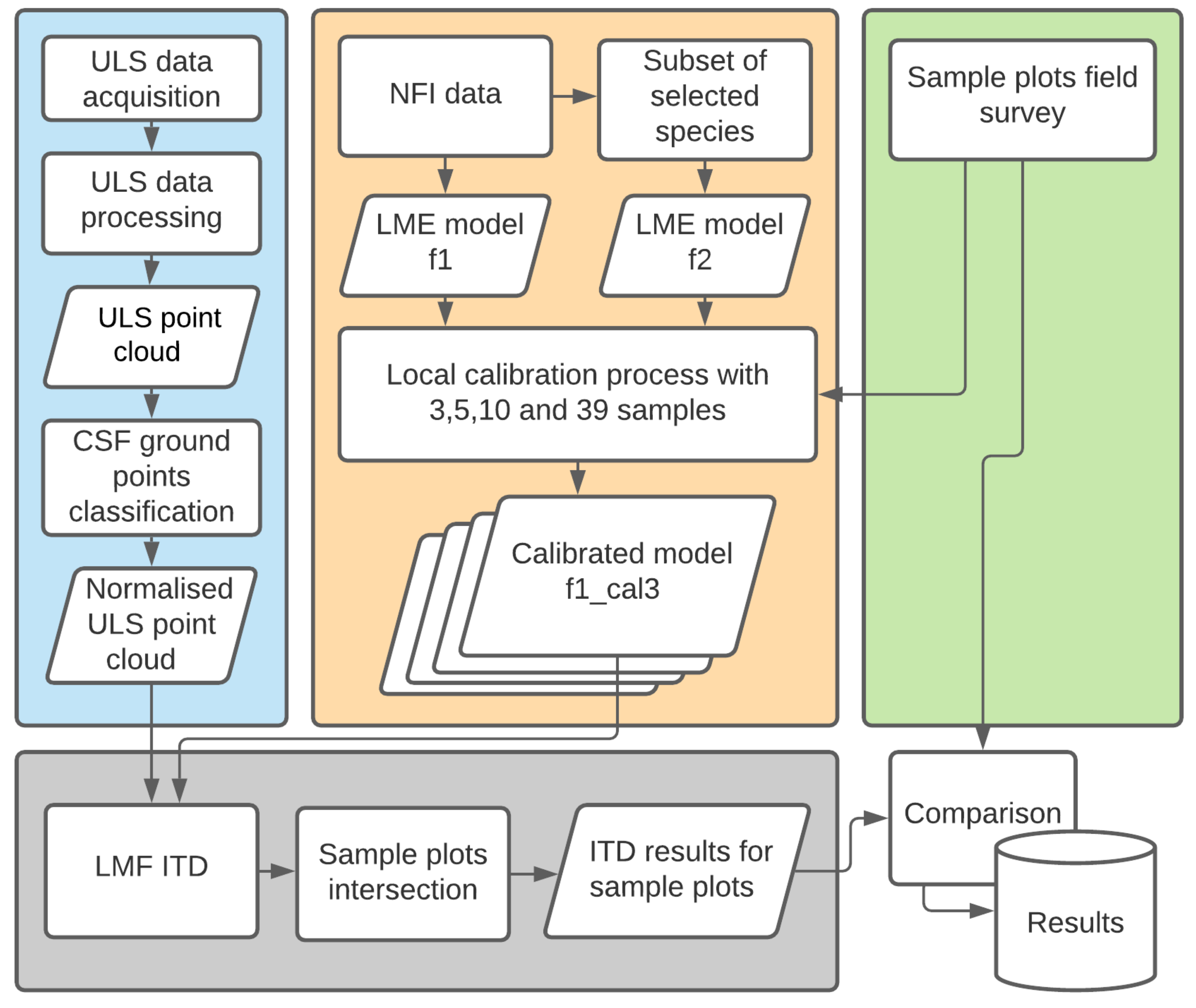
i.An overview of all of the processes described above part by part, leading to final results, is provided in
Figure 2. The model calibration test is not included in this flow chart.
All of the analyses were conducted in R-Studio version 1.4.1103 [
17] with R version 4.0.3 [
3] and using the following libraries: LidR [
4], ForestTools [
15], sjPlot [
18], JTools [
19], Readr [
20], GGplot2 [
21], and gtsummary [
22].
3. Results
3.2. Model Calibration Test
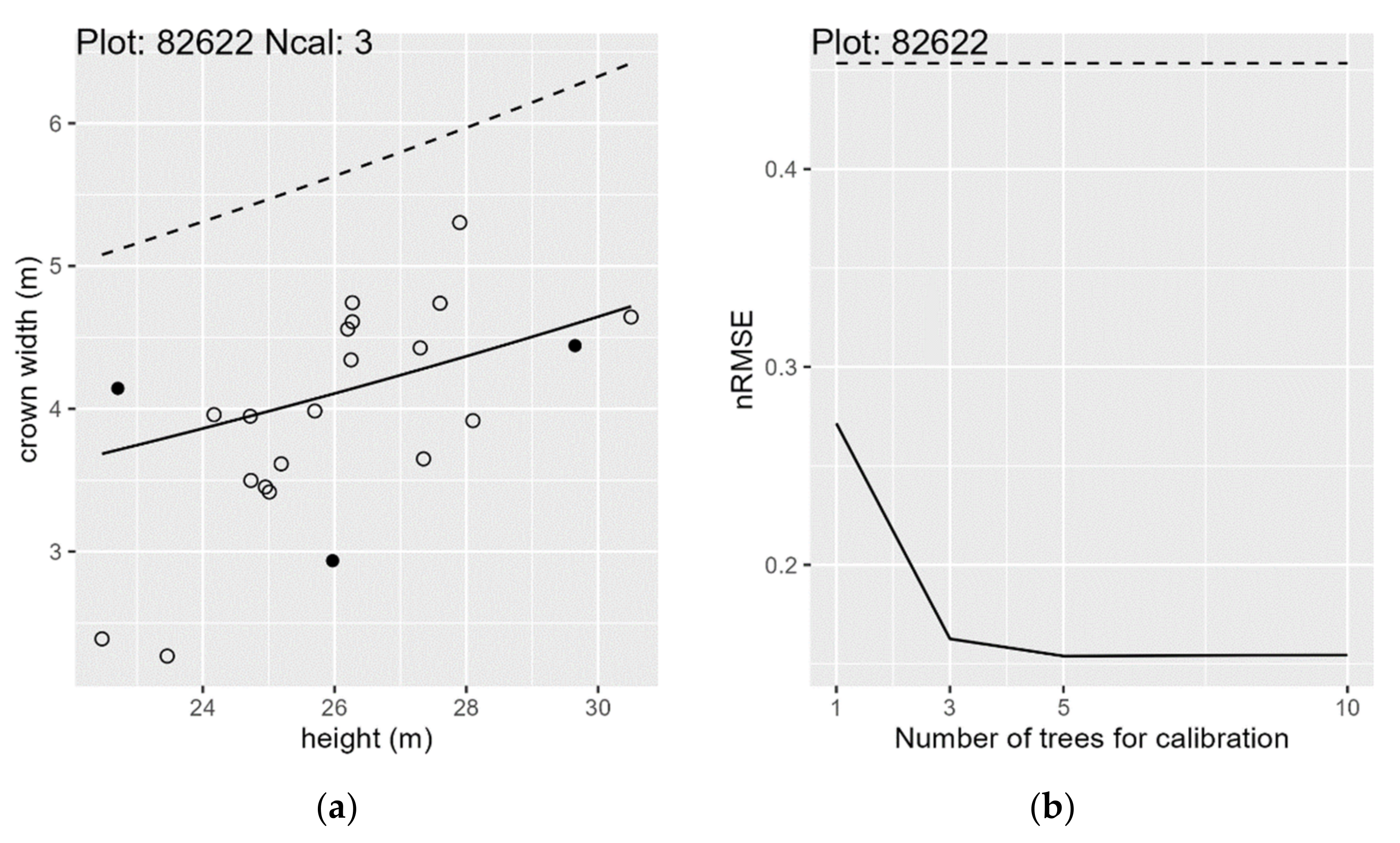
Using the local calibration procedure, a single plot from the NFI dataset (randomly selected from plots with more than 15 trees measured) was used as a hypothetical new plot. The model was calibrated repeatedly so that the model could be fit to the rest of the data set using 1, 3, 5, or 10 trees from the calibration plot. For each of these calibrated models, the crown width was estimated and compared to the original values from the NFI dataset
Figure 3.
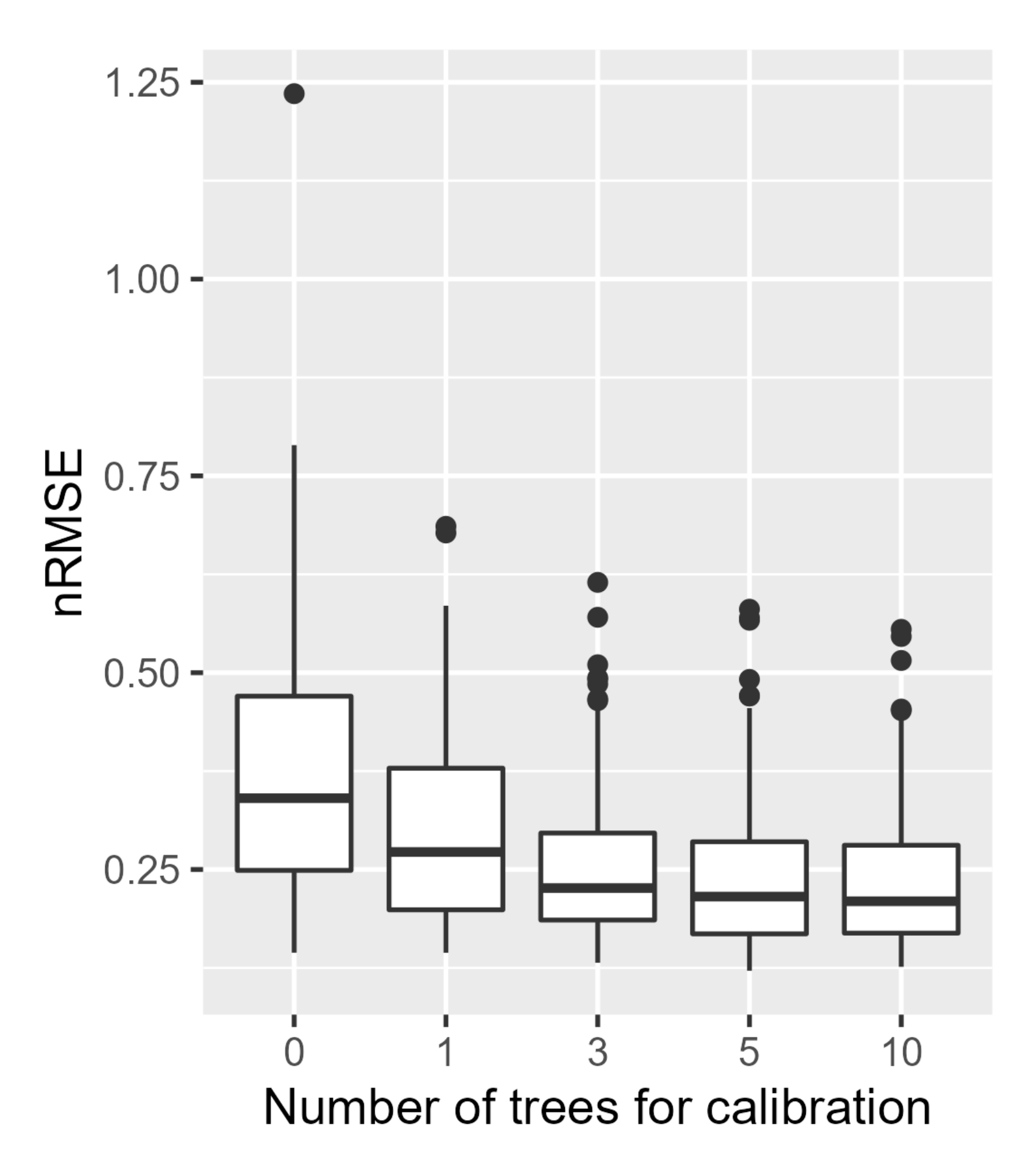
This procedure was repeated one hundred times. The overall performance of the calibration process is evident in
Figure 4, which shows that the model has a better fit when calibrated with more sample trees, although differences when using 3, 5, and 10 sample trees were relatively small. Using this procedure, it is evident that the fixed-effects model could be improved by the calibration process.
A Kruskal–Wallis test was conducted on the
nRMSE values based on the number of samples used for calibration and demonstrated a significant difference between groups (
p-value = 1.219 × 10
−13). Subsequently, Dunn’s test confirmed the optimal use of at least three samples for calibration; further increases in the sample numbers did not contribute any significant improvements, as seen in
Table 4.
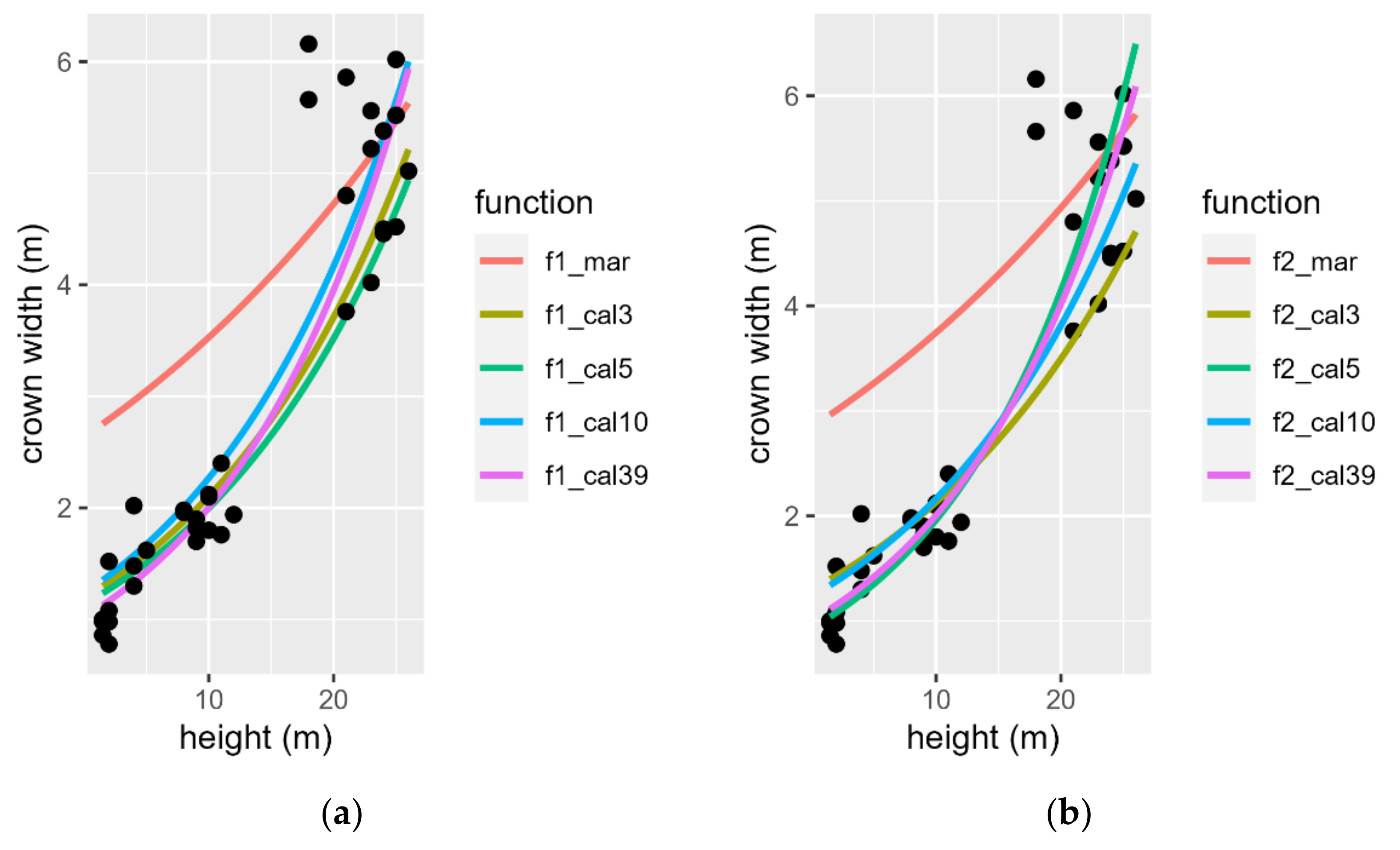
3.3. Study Site Model Calibration
A similar procedure was used for the local calibration of model f1 and f2 based on the data obtained from the sample plots at the study site. Again, several versions with 3, 5, 10, and the complete set of field-measured tree samples (39) were assessed. Together with the uncalibrated fixed-effects model, 10 formulas were produced overall to model crown widths based on tree heights, as seen in
Figure 5 and
Appendix A.
3.4. Tree Identification
The
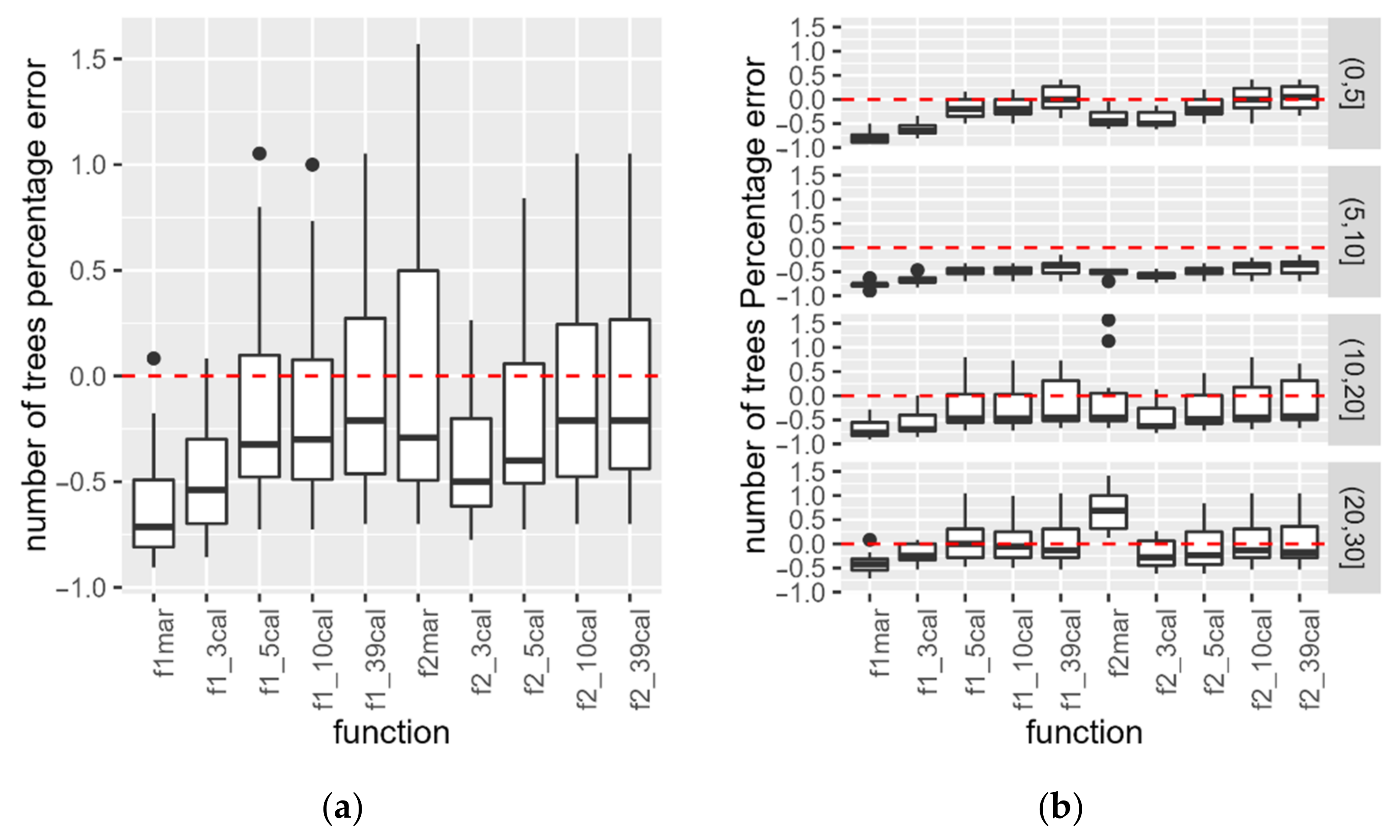
MPE between the field survey-observed and LMF-identified number of trees on the sample plots was −0.23 on average, varying from −0.62 to 0.04 (standard deviation of 0.21). The
nRMSE had values between 0.50 and 0.78. The MPE distribution determined by the function used for the LMF procedure is described in
Figure 6a, which indicates better results for calibrated functions overall, with the surprising exception of the fixed-effects only model for
Pinus and
Quercus spp., f2mar.
To better asses the influence of tree height, sample plots were divided into four consecutive categories according to max height of the trees observed in the plots.
Figure 6b and
Table 5 reveal that the unexpectedly good performance demonstrated by the f2mar function is the result of overestimating the number of the tallest trees on one hand and underestimating the number of the smallest trees on the other.
Table 5 also displays the increased accuracy of the calibrated models—with 5- and 10-sample calibrations showing comparable performance to the full 39-sample calibration. According to
nRMSE, the best performing model, f2_39cal, is closely followed by all models when 5 or more samples are used for calibration. In terms of height categories, the most underestimated category was the number of trees that were 5 to 10 m in height.
A Kruskal–Wallis test suggested significant differences in the tree count error determined by the model functions used for LMF (
p-value = 9.302 × 10
−6). A subsequent Dunn’s test revealed a significant improvement in the results when at least five samples were used for calibration (
Table 6). Using model f2, which was only fitted to data from the tree species present in the study site, did not bring expected improvements to any of the models.
4. Discussion
Iterative local calibration tests of a global LME model revealed significant improvements in model performance, even when only a single calibration sample was used. Three samples were interpreted to be the optimal amount because further increases in the number of samples did not create significant improvements. Several studies have similarly recommended only a limited number of samples for the calibration of mixed-effect height–diameter models [
24,
25,
26].
The local maximum filter belongs to one of the most commonly used approaches for individual tree top detection in point clouds [
1]. Determining the appropriate window size for LMF is often a trial-and-error process for particular stands or situations. The presented study tries to improve this situation by using a tree crown width that is to set the LMF window size.
Most reported approaches use other predictor variables, most often DBH, for crown projection rather than height [
5,
27,
28] and thus disqualifies using those models for local maximum filter techniques to detect individual tree tops.
Our suggested approach using a linear mixed-effects model to predict the tree crown width based on tree height using a few samples (results at our study site suggested at least five) that were obtained at the study site for local calibration might serve as a viable option. Our presented model reached a conditional R-square value of 0.70, which seems more promising than that obtained for a similar model built on a much smaller data sample, which had an R-square value of 0.51 [
2].
With the proposed LMF individual tree-detection method based on the crown width-determined window size using ULS point cloud data, an
nRMSE of around 0.50 was achieved. The
MPE metric, ranging between −0.62 and +0.03, revealed that in most cases, our approach led to a lower number of trees identified compared to the field survey. This can be attributed to the problematic distinction of single trees in
Pinus and
Quercus forest types, in our study site with a diverse tree structure. Not all of the trees have grown into the canopy layer, and the distinction of those trees is rather difficult, especially with broadleaved species. This is also supported by the poor performance of trees between 5 and 10 m. Somewhat similar tree detection results ranging from 50% to 140% using different ITD on ULS point cloud methods were reported by Wang et al. [
12]. A study by Grznárová et al. [
29] produced a detection rate of 95% for coniferous forests and a rate of 71% in broadleaved forests. Nevalainen et al. [
30] achieved tree identification rates between 64 and 97%. Results with 38 to 85% of trees undetected across plots were also reported by Jeronimo et al. [
31], who also reported that smaller trees were unable to be detected with the same level of success. Throughout the cited studies, it is clearly visible that ITD precision decreases with increased forest structure complexity.
5. Conclusions
The idea of using crown width to set the LMF window size seems to be logically justified. Still, correctly estimating the crown width based on tree height alone poses a significant challenge, as other influential factors, such as tree species, genetic variability, DBH, stand and site characteristics, etc. cannot be directly addressed in LMF. The locally calibrated mixed-effects model built on an extensive NFI dataset represents an approach that strives to cover all these other factors using the plot itself as a random effect.
Our individual tree top detection results only reached limited accuracy in terms of the number of trees identified in the sample plots. On the other hand, these results are comparable to those obtained in other research and suggest that the presented approach using a local maximum filter with a variable window size governed by locally calibrated models predicting crown width from tree height might serve as a universal point of departure when searching for optimal window size settings in LMF procedures and can provide reasonable accuracy, even in more complex forest structure.
Author Contributions
Conceptualization, J.K. and P.S.; methodology, J.K.; software, J.K.; validation, J.K. and P.S.; formal analysis, J.K. and P.S.; investigation, J.K.; resources, J.K.; data curation, J.K.; writing—original draft preparation, J.K.; writing—review and editing, J.K. and P.S.; visualization, J.K.; supervision, P.S.; project administration, J.K.; funding acquisition, P.S. All authors have read and agreed to the published version of the manuscript.
Funding
NAZV QK21010354 Progressive methods of forest management planning to support sustainable forest management.
Institutional Review Board Statement
Not applicable.
Informed Consent Statement
Not applicable.
Data Availability Statement
Not applicable.
Acknowledgments
The authors would like to thank the Forest Management Institute for providing data from the National Forest Inventory, and, from the same organization, Radim Adolt, for consultations regarding the mixed-effect models as well as to Jiří Nechvíle, Jan Máslo, Zdeněk Link, and Josef Málek for surveying the sample plots. Additionally, our colleagues from the Faculty of Forestry and Wood Sciences, namely Martin Slavík and Karel Kuželka, are thanks for the airborne laser scanning data acquisition.
Conflicts of Interest
The authors declare no conflict of interest.
Appendix A. Models Results
Table A1.
Model f1 (all species) details.
Table A1.
Model f1 (all species) details.
| | ln(CW) |
|---|
| Predictors | Estimates | CI | p |
|---|
| (Intercept) | 0.969152827 | 0.9551970430–0.9831086099 | <0.001 |
| H/100 | 2.919216056 | 2.8670704505–2.9713616608 | <0.001 |
| Random Effects |
| σ2 | 0.057922577 |
| τ00 | 0.324824782 |
| τ11 | 3.035113571 |
| ρ01 | −0.8865128648 |
| ICC | 0.609006432 |
| N pid | 22,532 |
| Observations | 94,066 |
| Marginal R2/Conditional R2 | 0.226/0.697 |
Table A2.
Model f2 (pine and oaks only) details.
Table A2.
Model f2 (pine and oaks only) details.
| | ln(CW) |
|---|
| Predictors | Estimates | CI | p |
|---|
| (Intercept) | 1.047111777 | 1.0140393762–1.0801841773 | <0.001 |
| H/100 | 2.749403592 | 2.6133807717–2.8854264117 | <0.001 |
| Random Effects |
| σ2 | 0.058775643 |
| τ00 | 0.379190163 |
| τ11 | 4.70297563 |
| ρ01 | −0.8577703035 |
| ICC | 0.666283129 |
| N pid | 7009 |
| Observations | 20,419 |
| Marginal R2/Conditional R2 | 0.129/0.709 |
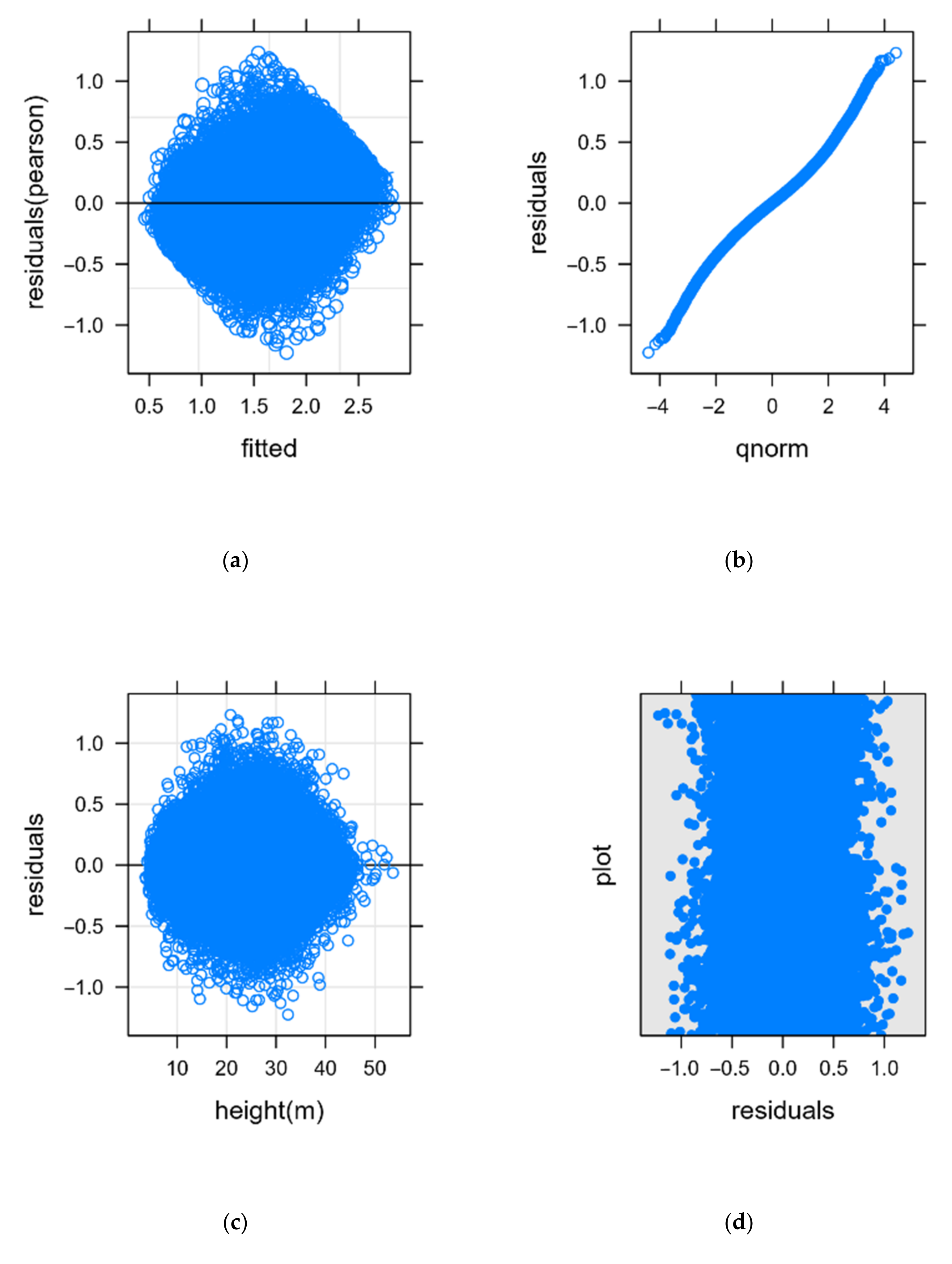
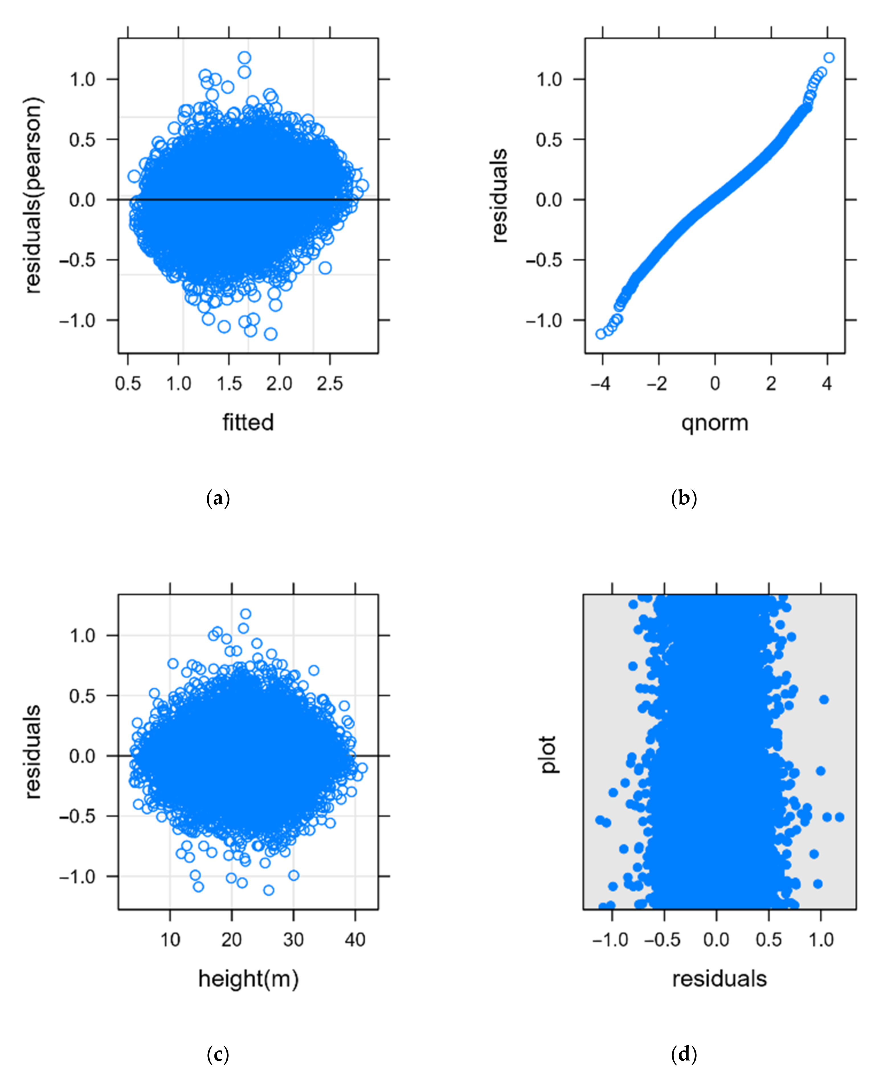
Figure A1.
Model f1 diagnostic plots (a) Tukey-Anscombe plot; (b) Q-Q plot; (c) residuals against fixed effect (height); (d) residuals against random effect (plot id).
Figure A1.
Model f1 diagnostic plots (a) Tukey-Anscombe plot; (b) Q-Q plot; (c) residuals against fixed effect (height); (d) residuals against random effect (plot id).
Figure A2.
Model f2 diagnostic plots (a) Tukey-Anscombe plot; (b) Q-Q plot; (c) residuals against fixed effect (height); (d) residuals against random effect (plot id).
Figure A2.
Model f2 diagnostic plots (a) Tukey-Anscombe plot; (b) Q-Q plot; (c) residuals against fixed effect (height); (d) residuals against random effect (plot id).
References
- Ke, Y.; Quackenbush, L.J. A Review of Methods for Automatic Individual Tree-Crown Detection and Delineation from Passive Remote Sensing. Int. J. Remote Sens. 2011, 32, 4725–4747. [Google Scholar] [CrossRef]
- Popescu, S.C.; Wynne, R.H.; Nelson, R.F. Estimating Plot-Level Tree Heights with Lidar: Local Filtering with a Canopy-Height Based Variable Window Size. Comput. Electron. Agric. 2003, 37, 71–95. [Google Scholar] [CrossRef]
- R Core Team R: A Language and Environment for Statistical Computing. Available online: https://www.r-project.org/ (accessed on 11 December 2021).
- Roussel, J.-R.; Auty, D. LidR: Airborne LiDAR Data Manipulation and Visualization for Forestry Applications. Available online: https://cran.r-project.org/package=lidR (accessed on 25 October 2021).
- Fu, L.; Sun, H.; Sharma, R.P.; Lei, Y.; Zhang, H.; Tang, S. Nonlinear Mixed-Effects Crown Width Models for Individual Trees of Chinese Fir (Cunninghamia Lanceolata) in South-Central China. For. Ecol. Manage. 2013, 302, 210–220. [Google Scholar] [CrossRef]
- Gill, S.J.; Biging, G.S.; Murphy, E.C. Modeling Conifer Tree Crown Radius and Estimating Canopy Cover. For. Ecol. Manage. 2000, 126, 405–416. [Google Scholar] [CrossRef] [Green Version]
- Bechtold, W.A. Crown-Diameter Prediction Models for 87 Species of Stand-Grown Trees in the Eastern United States. South. J. Appl. For. 2003, 27, 269–278. [Google Scholar] [CrossRef] [Green Version]
- Lappi, J. Calibration of Height and Volume Equations with Random Parameters. For. Sci. 1991, 37, 781–801. [Google Scholar]
- Lynch, T.B.; Holley, A.G.; Stevenson, D.J. A Random-Parameter Height-Dbh Model for Cherrybark Oak. South. J. Appl. For. 2005, 29, 22–26. [Google Scholar] [CrossRef] [Green Version]
- Adolt, R.; Kučera, M.; Zapadlo, J.; Andrlík, M.; Čech, Z.; Coufal, J. Pracovní Postupy Pozemního Šetření NIL2; Ústav pro Hospodářskou Úpravu Lesů Brandýs nad Labem: Brandýs nad Labem, Czech Republic, 2013; ISBN 9788090542327. [Google Scholar]
- Kuželka, K.; Slavík, M.; Surový, P. Very High Density Point Clouds from UAV Laser Scanning for Automatic Tree Stem Detection and Direct Diameter Measurement. Remote Sens. 2020, 12, 1236. [Google Scholar] [CrossRef] [Green Version]
- Wang, Y.; Hyyppa, J.; Liang, X.; Kaartinen, H.; Yu, X.; Lindberg, E.; Holmgren, J.; Qin, Y.; Mallet, C.; Ferraz, A.; et al. International Benchmarking of the Individual Tree Detection Methods for Modeling 3-D Canopy Structure for Silviculture and Forest Ecology Using Airborne Laser Scanning. IEEE Trans. Geosci. Remote Sens. 2016, 54, 5011–5027. [Google Scholar] [CrossRef] [Green Version]
- Riegl RIEGL RIEGL VUX-SYS VUX-SYS Complete Sensor System for Kinematic Laser Scanning. Available online: http://www.riegl.com/uploads/tx_pxpriegldownloads/RIEGL_VUX-SYS_Datasheet_2020-10-02_01.pdf (accessed on 6 August 2021).
- Czech Republic Letecký Předpis L 2 Pravidla Létání; Ministerstvo Dopravy České Republiky: Prague, Czech Republic, 2020.
- Plowright, A.; Roussel, J.-R. ForestTools: Analyzing Remotely Sensed Forest Data. Available online: https://cran.r-project.org/package=ForestTools (accessed on 11 December 2021).
- Zhang, W.; Qi, J.; Wan, P.; Wang, H.; Xie, D.; Wang, X.; Yan, G. An Easy-to-Use Airborne LiDAR Data Filtering Method Based on Cloth Simulation. Remote Sens. 2016, 8, 501. [Google Scholar] [CrossRef]
- RStudio Team. RStudio: Integrated Development Environment for R. Available online: http://www.rstudio.com/ (accessed on 11 December 2021).
- Lüdecke, D. SjPlot: Data Visualization for Statistics in Social Science. Available online: https://cran.r-project.org/package=sjPlot (accessed on 11 December 2021).
- Long, J.A. Jtools: Analysis and Presentation of Social Scientific Data. Available online: https://cran.r-project.org/package=jtools (accessed on 11 December 2021).
- Wickham, H.; Hester, J. Readr: Read Rectangular Text Data. Available online: https://cran.r-project.org/package=readr (accessed on 11 December 2021).
- Wickham, H. Ggplot2: Elegant Graphics for Data Analysis. Available online: https://ggplot2.tidyverse.org (accessed on 11 December 2021).
- Sjoberg, D.D.; Whiting, K.; Curry, M.; Lavery, J.A.; Larmarange, J. Reproducible Summary Tables with the Gtsummary Package. R J. 2021, 13, 570–580. [Google Scholar] [CrossRef]
- Nakagawa, S.; Johnson, P.C.D.; Schielzeth, H. The Coefficient of Determination R2 and Intra-Class Correlation Coefficient from Generalized Linear Mixed-Effects Models Revisited and Expanded. J. R. Soc. Interface 2017, 14, 20170213. [Google Scholar] [CrossRef] [PubMed] [Green Version]
- Trincado, G.; VanderSchaaf, C.L.; Burkhart, H.E. Regional Mixed-Effects Height-Diameter Models for Loblolly Pine (Pinus Taeda L.) Plantations. Eur. J. For. Res. 2007, 126, 253–262. [Google Scholar] [CrossRef]
- Calama, R.; Montero, G. Stand and Tree-Level Variability on Stem Form and Tree Volume in Pinus Pinea L.: A Multilevel Random Components Approach. Investig. Agrar. Sist. Recur. For. 2006, 15, 24. [Google Scholar] [CrossRef] [Green Version]
- Jayaraman, K.; Lappi, J. Estimation of Height-Diameter Curves through Multilevel Models with Special Reference to Even-Aged Teak Stands. For. Ecol. Manage. 2001, 142, 155–162. [Google Scholar] [CrossRef]
- Condés, S.; Sterba, H. Derivation of Compatible Crown Width Equations for Some Important Tree Species of Spain. For. Ecol. Manage. 2005, 217, 203–218. [Google Scholar] [CrossRef]
- Sönmez, T. Diameter at Breast Height-Crown Diameter Prediction Models for Picea Orientalis. African J. Agric. Res. 2009, 4, 215–219. [Google Scholar]
- Grznárová, A.; Mokroš, M.; Surový, P.; Slavík, M.; Pondelík, M.; Merganič, J. The Crown Diameter Estimation from Fixed Wing Type of UAV Imagery. ISPRS-Int. Arch. Photogramm. Remote Sens. Spat. Inf. Sci. 2019, 42, 337–341. [Google Scholar] [CrossRef] [Green Version]
- Nevalainen, O.; Honkavaara, E.; Tuominen, S.; Viljanen, N.; Hakala, T.; Yu, X.; Hyyppä, J.; Saari, H.; Pölönen, I.; Imai, N.N.; et al. Individual Tree Detection and Classification with UAV-Based Photogrammetric Point Clouds and Hyperspectral Imaging. Remote Sens. 2017, 9, 185. [Google Scholar] [CrossRef] [Green Version]
- Jeronimo, S.M.A.; Kane, V.R.; Churchill, D.J.; McGaughey, R.J.; Franklin, J.F. Applying LiDAR Individual Tree Detection to Management of Structurally Diverse Forest Landscapes. J. For. 2018, 116, 336–346. [Google Scholar] [CrossRef] [Green Version]
| Publisher’s Note: MDPI stays neutral with regard to jurisdictional claims in published maps and institutional affiliations. |
© 2022 by the authors. Licensee MDPI, Basel, Switzerland. This article is an open access article distributed under the terms and conditions of the Creative Commons Attribution (CC BY) license (https://creativecommons.org/licenses/by/4.0/).


