High-Resolution ISAR Imaging Based on Plug-and-Play 2D ADMM-Net

Abstract

We propose a deep learning architecture, dubbed Plug-and-play 2D ADMM-Net (PAN), by combining model-driven deep networks and data-driven deep networks for effective high-resolution 2D inverse synthetic aperture radar (ISAR) imaging with various signal-to-noise ratios (SNR) and incomplete data scenarios. First, a sparse observation model of 2D ISAR imaging is established, and a 2D ADMM algorithm is presented. On this basis, using the plug and play (PnP) technique, PnP 2D ADMM is proposed, by combining the 2D ADMM algorithm and the deep denoising network DnCNN. Then, we unroll and generalize the PnP 2D ADMM to the PAN architecture, in which all adjustable parameters in the reconstruction layers, denoising layers, and multiplier update layers are learned by end-to-end training through back-propagation. Experimental results showed that the PAN with a single parameter set can achieve noise-robust ISAR imaging with superior reconstruction performance on incomplete simulated and measured data under different SNRs.

1. Introduction

High-resolution inverse synthetic aperture radar (ISAR) transmits a wide band signal to achieve a high resolution range profile and synthesizes a virtual aperture through the motion of the target, to achieve a high resolution along azimuth direction. Unlike optical imaging, ISAR has been used in various military applications, e.g., space situation awareness and air target surveillance in all-day and all-weather environments [1,2]. Generally, well-focused ISAR imaging can be obtained from high signal-to-noise ratio (SNR) and complete echoes using a range-Doppler (RD) algorithm and the polar formatting algorithm (PFA) [3]. In practice, the long observation distance in a low-elevation angle environment may generate low SNR. Additionally, in complex electromagnetic environments with active interference and passive interference, the non-cooperative nature of target and radar resource scheduling [4] may result in incomplete echoes, and the available imaging algorithms based on Fourier analysis cannot obtain satisfactory results. Considering the sparse nature of the scattering centers in the image domain, high-resolution ISAR imaging based on sparse signal reconstruction has received intensive attention in recent years [5,6].

The sparse signal reconstruction methods convert the sparse ISAR imaging problem into a sparse signal reconstruction problem, and then search the optimal solution by $l_0$-norm and $l_1$-norm optimizations. The $l_0$-norm optimization, such as orthogonal matching pursuit (OMP) [7] and smoothed L0 (SL0) [8] are sensitive to noise and prone to local optima. For $l_1$-norm optimization, a fast iterative shrinkage-thresholding algorithm (FISTA) [9] and alternating direction method of multipliers (ADMM) [10] can guarantee the sparsest solution. However, these methods usually require careful tuning of the regularization parameters, which is still an open problem. For 2D imaging, the vectorized optimization required a long operational time and large memory storage space. To tackle this problem, 2D SL0 [11], 2D FISTA [12], and 2D ADMM [13] based on matrix operations are proposed. Although the abovementioned sparse signal reconstruction methods have a clear physical significance and strong theoretical support, their performance will degrade rapidly, due to improper parameter setup.

Apart from traditional optimization methods, deep networks have recently provided unprecedented performance gains in ISAR imaging. The available deep networks mainly include: (1) model-driven methods, and (2) data-driven methods. Model-driven methods are generally based on the unrolling technique, which was first proposed by expanding the iterative shrinkage-thresholding (ISTA) algorithm, to improve the computational efficiency of sparse coding algorithms through end-to-end training [14]. Specifically, in ISAR imaging, the model-driven methods expand the iterative steps of the sparse signal reconstruction method into a deep network with finite-layers, set the adjustable parameters as network parameters, and then obtain their optimal values by network training. Finally, they output the focused image of an unknown target from the trained network. Typical networks with model-driven methods include AF-AMPNet [15], 2D-ADMM-Net (2D-ADN) [16], and convolution iterative shrinkage-thresholding (CIST) [17], etc. Although model-driven methods have strong interpretability and satisfying reconstruction performance, the optimal parameters are sensitive to SNR. Therefore, to obtain a well-focused image under various SNRs, it is necessary to build a model set, which will increase the time and space complexity.

The data-driven methods directly learn the nonlinear mapping between the input (e.g., the RD image) and the label image, to achieve high-resolution imaging by designing and training deep networks. Facilitated by off-line network training, these methods can reconstruct multiple images rapidly. Typical ones in data-driven methods include fully convolutional neural network (FCNN) [18] and UNet [19], etc. The data-driven methods generally adopt a hierarchical architecture composed of many layers and a large number of parameters (possibly millions); thus, they are capable of learning complicated mappings [14]. Specifically, in ISAR imaging, they have demonstrated robustness to various noise levels, i.e., a single trained network can achieve well-focused imaging of echoes with various SNR. However, the subjective network design process lacks unified criterion and theoretical support, which makes it difficult to analyze the influence of network structure and parameter settings on the reconstruction performance. In addition, they usually suffer from poor generalization performance and fail to obtain satisfying imaging results with incomplete data, as will be demonstrated later in Section 5.

Plug-and-play (PnP) [20] is a non-convex framework that combines proximal algorithms with advanced denoiser priors [21], e.g., block-matching and 3D filtering (BM3D) [22] or deep denoising network DnCNN [23]. Recently, PnP has achieved great empirical success in a large variety of imaging applications [24,25,26,27], owing to its effectiveness and flexibility, especially with the integration of a deep denoising network. Compared with the original iterative methods, PnP methods offer more promising imaging results, due to their powerful denoising performance. However, PnP is highly sensitive to parameter selection. In addition, parameter tuning requires several trials, which is cumbersome and time-consuming.

To tackle the abovementioned issues, this article proposes plug-and-play 2D ADMM-Net (PAN), for high-resolution 2D ISAR imaging in complex environments. The key contributions include the following:

• 2D ADMM algorithm for sparse ISAR imaging is derived. On this basis, PnP 2D ADMM is proposed by combining a deep denoising network DnCNN and the 2D ADMM algorithm, which can significantly improve reconstruction performance.
• To tackle the issues of parameter selection and tuning in PnP 2D ADMM, PAN, which is derived from PnP 2D ADMM, is designed using the ‘unrolling’ technique. Particularly, the adjustable parameters are estimated through end-to-end training. By this means, the sensitivity of the model-driven deep network to noise and the poor performance of the data-driven deep network for incomplete data are effectively addressed.
• Although PAN is only trained by simulated data, experiments have shown that it can be generalized to measured data with different SNRs and obtain well-focused imaging.

The remainder of this article is organized as follows: Section 2 establishes the sparse ISAR observation model, provides the iterative formulae of 2D ADMM, and proposes the PnP 2D ADMM for high-resolution 2D imaging. Section 3 introduces the structure of PAN in detail. Section 4 introduces the training of PAN in detail. Section 5 carries out various experiments to prove the effectiveness of PAN. Section 6 discusses the depth of PAN, and Section 7 concludes the article with suggestions for future work.

2. Modeling and Solving

2.1. Signal Model

In ISAR imaging, the instantaneous range of a target can be seen as a combination of translational and rotational motion, in which the former is not beneficial to imaging and needs to be compensated by range alignment and autofocusing. Therefore, after translational motion compensation, it is supposed that the target is uniformly rotating.

The ISAR transmits a linear-frequency-modulated (LFM) signal with a high time-bandwidth product, which can be modeled as

$$s\left(\widehat{t},t_m\right)=rect\left(\frac{\widehat{t}}{T_p}\right)\exp \left(j2\pi \left(f_{c}t+\frac{1}{2}\gamma {\widehat{t}}^2\right)\right)$$

(1)

where $rect\left(u\right)=\{\begin{array}{c}1,\left|u\right|\le 1/2\\ 0,\left|u\right|>1/2\end{array}$ denotes the window function. $f_c$, $T_p$, and $\gamma$ denote the carrier frequency, pulse width, and chirp rate, respectively. The full time $t=\widehat{t}+t_m$ is expressed in the form of fast time $\widehat{t}$ and slow time $t_m=m/\mathrm{PRF}$, where $m$ is the azimuth index and $\mathrm{PRF}$ represents pulse repetition frequency. Supposing that the target motion only changes with the slow time and there are $P$ scatters on the target, the received echoes can be expressed as

$$\begin{array}{c}{s}_R\left(\widehat{t},t_m\right)={\displaystyle \sum _{p=1}^P{A}_{p}rect\left(\frac{\widehat{t}-\left(2R_p\left(t_m\right)/c\right)}{T_p}\right)}\\ \hspace{1em}\hspace{1em}\hspace{1em}\hspace{1em}\times \exp \left(j2\pi \left(f_c\left(\widehat{t}-\frac{2R_p\left(t_m\right)}{c}\right)+\frac{1}{2}\gamma {\left(\widehat{t}-\frac{2R_p\left(t_m\right)}{c}\right)}^2\right)\right)\end{array}$$

(2)

where $A_p$, $R_p\left(t_m\right)$ denote the backscattering coefficient of the $p$th scatterer and its instantaneous range to the radar, respectively.

After dechirping, the echoes in the range frequency-slow time can be expressed as follows:

$$s\left(f,t_m\right)={\displaystyle \sum _{p=1}^P{A}_{p}rect\left(\frac{f}{B}\right)\exp \left(-j\frac{4\pi }{c}\left(f_c+f\right)R_{ps}\left(t_m\right)\right)}$$

(3)

where $f\in \left[-B/2,B/2\right]$ is the range frequency, $B$ is the bandwidth, and $R_{ps}$ is the instantaneous slant range between the $p$th scattering center and the reference point.

For a target that rotates by a small angle during the imaging interval, or for echoes after migration through range cell correction, we have

$$R_{ps}=x_p+y_p{\omega }_{rot}{t}_m$$

(4)

where $x_p$ and $y_p$ represent the location of the $p$th scattering center on the reference coordinate. ${\omega }_{rot}$ is the angular rotation frequency of the turntable model.

For sparse band and azimuth observation, after translational motion compensation, an echo $s\left(f,t_m\right)$ can be written in a matrix form $Y\in {ℂ}^{M\times N}$ after discretization, and (4) can be rewritten as

$$Y={\Phi }_{1}X{\Phi }_2+N$$

(5)

where ${\Phi }_1\in {ℂ}^{M\times U}$ is the range dictionary with $M<U$, $X\in {ℂ}^{U\times V}$ is the 2D distribution of scattering centers, i.e., the image to be reconstructed, ${\Phi }_2\in {ℂ}^{V\times N}$ is the Doppler dictionary with $N<V$, and $N\in {ℂ}^{M\times N}$ is the complex noise matrix.

2.2. The 2D ADMM Method

Solving $X$ from Equation (6) is a typical linear inverse problem, which can be converted into an $l_1$-norm optimization in a matrix form, i.e.,

$$\underset{X}{\min }\left\{\frac{1}{2}{\Vert Y-{\Phi }_{1}X{\Phi }_2\Vert }_F^2+\lambda {\Vert X\Vert }_1\right\}$$

(6)

where $\lambda$ is the regularization parameter, which has a great impact on imaging performance.

As a commonly used $l_1$-norm optimization method, 2D ADMM has good reconstruction performance for linear inverse problems. By introducing an auxiliary matrix $Z$, (6) can be expressed as

$$\begin{array}{l}\underset{X}{\min }\left\{\frac{1}{2}{\Vert Y-{\Phi }_{1}X{\Phi }_2\Vert }_F^2+\lambda {\Vert Z\Vert }_1\right\}\\ s.t.X-Z=0\end{array}$$

(7)

To solve this constrained optimization problem, 2D ADMM utilizes the augmented Lagrangian method, where the augmented Lagrangian function is

$$ℒ\left(X,Z,\mathbb{A}\right)=\frac{1}{2}{\Vert Y-{\Phi }_{1}X{\Phi }_2\Vert }_F^2+\lambda {\Vert Z\Vert }_1+\langle \mathbb{A},X-Z\rangle +\frac{\rho }{2}{\Vert X-Z\Vert }_F^2$$

(8)

where $\mathbb{A}$ is the Lagrangian multipliers and $\rho$ is the penalty parameter, which should be carefully adjusted to obtain better imaging results.

According to the principles of the 2D ADMM algorithm, Equation (8) was decomposed into three sub-problems by minimizing $ℒ\left(X,Z,\mathbb{A}\right)$ with respect to $X$, $Z$, and $\mathbb{A}$, respectively,

$$\{\begin{array}{c}{X}^{\left(n\right)}=\underset{X}{\arg \min }\frac{1}{2}{\Vert Y-{\Phi }_{1}X{\Phi }_2\Vert }_F^2+\langle {\mathbb{A}}^{\left(n-1\right)},X-Z^{\left(n-1\right)}\rangle +\frac{\rho }{2}{\Vert X-Z^{\left(n-1\right)}\Vert }_F^2\\ Z^{\left(n\right)}=\underset{Z}{\arg \min }\lambda {\Vert Z\Vert }_1+\langle {\mathbb{A}}^{\left(n-1\right)},X^{\left(n\right)}-Z\rangle +\frac{\rho }{2}{\Vert X^{\left(n\right)}-Z\Vert }_F^2\\ {\mathbb{A}}^{\left(n\right)}={\mathbb{A}}^{\left(n-1\right)}+\rho \left(X^{\left(n\right)}-Z^{\left(n\right)}\right)\end{array}$$

(9)

where $n$ is the iteration index. Let $\mathbb{B}=\frac{\mathbb{A}}{\rho }$, then the solution to (9) satisfy,

$$X^{\left(n\right)}=\left(Z^{\left(n-1\right)}-{\mathbb{B}}^{\left(n-1\right)}\right)-\frac{1}{1+\rho }{\Phi }_1^{\mathrm{H}}\left({\Phi }_1\left(Z^{\left(n-1\right)}-{\mathbb{B}}^{\left(n-1\right)}\right){\Phi }_2-Y\right){\Phi }_2^{\mathrm{H}}$$

(10)

$$Z^{\left(n\right)}=S\left(X^{\left(n\right)}+{\mathbb{B}}^{\left(n-1\right)};\lambda /\rho \right)$$

(11)

$${\mathbb{B}}^{\left(n\right)}={\mathbb{B}}^{\left(n-1\right)}+\eta \left(X^{\left(n\right)}-Z^{\left(n\right)}\right)$$

(12)

where $S(\cdot )$ is the shrinkage function, and $\eta$ is the update rate for the Lagrangian multiplier.

It is worth mentioning that the optimal parameters of the 2D ADMM are sensitive to SNR. Therefore, several trials are required to obtain well-focused imaging, making this method impractical and time-consuming.

2.3. PnP 2D ADMM Method

The soft threshold function in Formula (12) can be treated as a denoising procedure and henceforth be replaced by a pre-trained deep denoising network through the PnP framework,

$$Z^{\left(n\right)}=D\left(X^{\left(n\right)}+{\mathbb{B}}^{\left(n-1\right)}\right)$$

(13)

where $D(\cdot )$ represents the pre-trained deep denoising network. In this article, we chose DnCNN due to its satisfying denoising performance.

Algorithm 1 summarizes the high-resolution 2D ISAR imaging method based on PnP 2D ADMM, where $N$ denotes the total number of iterations.

Algorithm 1: High-Resolution ISAR Imaging Based on PnP 2D ADMM.

$1.\mathrm{Initialize}\rho >0,Z^{\left(0\right)},\mathrm{and}{\mathbb{B}}^{\left(0\right)};$

$2.\mathrm{For}n=1:N$

$\hspace{1em}\hspace{1em}\hspace{1em}\mathrm{Update}{X}^{\left(n\right)}\mathrm{by}\left(10\right);$

$\hspace{1em}\hspace{1em}\hspace{1em}\mathrm{Update}{Z}^{\left(n\right)}\mathrm{by}\left(13\right);$

$\hspace{1em}\hspace{1em}\hspace{1em}\mathrm{Update}{\mathbb{B}}^{\left(n\right)}\mathrm{by}\left(12\right);$

End

$3.\mathrm{Output}{X}^{\left(N+1\right)}\mathrm{by}\left(10\right).$

Although the reconstruction performance and noise robustness of the PnP 2D ADMM can be significantly improved by adopting DnCNN as the denoising prior, the choice of $\rho$ and $\eta$ still has a large impact on the image quality, and improper initialization may generate defocused images.

To obtain well-focused imaging, we need to find the optimal parameters manually through several trials. In addition, the internal parameter cannot be adjusted adaptively in each iteration, which lacks flexibility and leads to slow convergence.

3. Structure of PAN

To tackle the issue of the optimal internal parameter selection of the PnP 2D ADMM, we modify the structure of PnP 2D ADMM and expand it into a learnable deep architecture, i.e., the PAN, employing the unrolling technique. As shown in Figure 1, the network has $N$ stages, and Stage $n$, $n\in \left[1,N\right]$, represents the $n$th iteration described by

Table 1. Performance evaluation for the simulated 2D incomplete data under 5 dB condition.

Method	NMSE	PSNR	SSIM	Time(s)
UNet	0.4665	40.9056	0.9579	0.01
2D-ADN	0.1728	49.5218	0.9897	0.09
PnP 2D ADMM	0.2286	47.4149	0.9805	1.12
PAN	0.2035	48.1073	0.9847	0.01

. Typically, one stage consists of three layers, i.e., the reconstruction layer $R\left(\cdot ,\cdot ,\cdot ;{\rho }^{\left(n\right)}\right)$; the denoising layer $D\left(\cdot ,\cdot ;w^{\left(n\right)}\right)$, where $w$ is the network parameter; and the multiplier update layer $U\left(\cdot ,\cdot ,\cdot ;{\eta }^{\left(n\right)}\right)$. The three layers correspond to (10), (13), and (12), respectively. In addition, $(\cdot )$ represents the inputs of each layer. By these means, the penalty parameters and the update rate are trainable and the internal parameters are adjustable in each iteration.

3.1. Reconstruction Layer

The inputs of the reconstruction layer are the output of the denoising layer $Z^{\left(n-1\right)}$ and the multiplier update layer ${\mathbb{B}}^{\left(n-1\right)}$, and the output of the reconstruction layer is

$$X^{\left(n\right)}=\left(Z^{\left(n-1\right)}-{\mathbb{B}}^{\left(n-1\right)}\right)-\frac{1}{1+{\rho }^{\left(n\right)}}{\Phi }_1^{\mathrm{H}}\left({\Phi }_1\left(Z^{\left(n-1\right)}-{\mathbb{B}}^{\left(n-1\right)}\right){\Phi }_2-Y\right){\Phi }_2^{\mathrm{H}}$$

(14)

where ${\rho }^{\left(n\right)}$ is the adjustable network parameter.

For $n=1$, $Z^{\left(0\right)}$ and ${\mathbb{B}}^{\left(0\right)}$ are initialized to zero matrices and, thus, Equation (14) can be rewritten as

$$X^{\left(1\right)}=-\frac{1}{1+{\rho }^{\left(1\right)}}{\Phi }_1^{\mathrm{H}}\left(-Y\right){\Phi }_2^{\mathrm{H}}$$

(15)

For $n\in \left[1,N\right]$, the output of the reconstruction layer serves as the input of the denoising layer $Z^{\left(n\right)}$ and the multiplier update layer ${\mathbb{B}}^{\left(n\right)}$. For $n=N+1$, the output of the reconstruction layer is the input of the loss function.

3.2. Denoising Layer

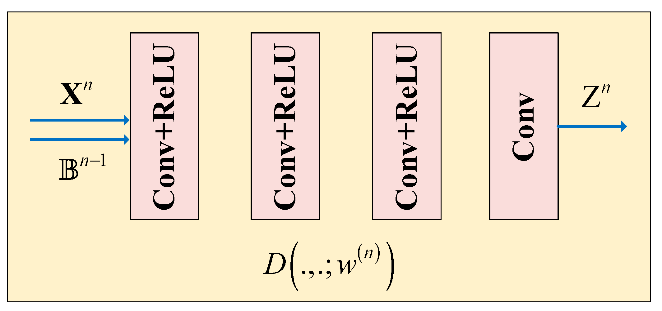
As shown in Figure 2, the inputs of the denoising layer are the output of the reconstruction layer $X^{\left(n\right)}$ and the previous multiplier update layer ${\mathbb{B}}^{\left(n-1\right)}$, and the output of the denoising layer is

$$Z^{\left(n\right)}=D\left(X^{\left(n\right)}+{\mathbb{B}}^{\left(n-1\right)};w^{\left(n\right)}\right)$$

(16)

where the deep network $D\left(\cdot ,\cdot ;w^{\left(n\right)}\right)$ is DnCNN, without residual learning and batch normalization. As shown in Figure 2, the first three layers are convolution layers followed by the ReLU activation function, and each layer has 64 convolution kernels with the same kernel size $3\times 3$. In addition, we add a convolutional layer with one convolution kernel, whose size is $3\times 3$.

For $n=1$, ${\mathbb{B}}^{\left(0\right)}$ is initialized as a zero matrix and Equation (16) can be reduced to the following form,

$$Z^{\left(1\right)}=D\left(X^{\left(1\right)};w^{\left(1\right)}\right)$$

(17)

The output of the denoising layer is the input of the reconstruction layer $X^{\left(n+1\right)}$ and the multiplier update layer ${\mathbb{B}}^{\left(n\right)}$.

3.3. Multiplier Update Layer

The inputs of the multiplier update layer are the output of the previous multiplier update layer ${\mathbb{B}}^{\left(n-1\right)}$, the reconstruction layer $X^{\left(n\right)}$, and the denoising layer $Z^{\left(n\right)}$, and the output of the multiplier update layer is

$${\mathbb{B}}^{\left(n\right)}={\mathbb{B}}^{\left(n-1\right)}+{\eta }^{\left(n\right)}\left(X^{\left(n\right)}-Z^{\left(n\right)}\right)$$

(18)

where the update rate ${\eta }^{\left(n\right)}$ is the adjustable network parameter.

For $n=1$, ${\mathbb{B}}^{\left(0\right)}$ is initialized as a zero matrix and Equation (18) can be expressed as,

$${\mathbb{B}}^{\left(1\right)}={\eta }^{\left(1\right)}\left(X^{\left(1\right)}-Z^{\left(1\right)}\right)$$

(19)

For $n\in \left[1,N-1\right]$, the output of the multiplier update layer is the input of the next reconstruction layer $X^{\left(n+1\right)}$, the next denoising layer $Z^{\left(n+1\right)}$, and the next multiplier update layer ${\mathbb{B}}^{\left(n+1\right)}$. For $n=N$, the output of the multiplier update layer is the input of the next reconstruction layer.

4. Training of PAN

In this article, we train PAN according to the forward-backward propagation method. By this means, the error can be back-propagated to the entire network, to directly update all the adjustable parameters, i.e., the penalty parameters in the reconstruction layers, the parameters of DnCNN in the denoising layers, and the update rate in the multiplier update layers. Below, we will discuss network training in detail.

4.1. Loss Function

In this article, the normalized mean square error (NMSE) is used as the loss function $\mathbb{L}\left(\Theta \right)$, which satisfied,

$$\mathbb{L}\left(\Theta \right)=\frac{1}{\gamma }{\displaystyle \sum _{\left(Y,X^{gt}\right)\in \mathsf{\Gamma }}\frac{\sqrt{{\Vert \widehat{X}\left(Y,\Theta \right)-X^{gt}\Vert }_F^2}}{\sqrt{{\Vert X^{gt}\Vert }_F^2}}}$$

(20)

where $\widehat{X}$ is the network output, $Y$ is the input echoes in the wavenumber domain defined by (5), $\Theta =\left\{{\rho }^{\left(n\right)},w^{\left(n\right)},{\eta }^{\left(n\right)}\right\}$ is the set of adjustable parameters, $X^{gt}$ is the label image, ${\Vert \cdot \Vert }_F$ is the Frobenius norm, and $\mathsf{\Gamma }=\left\{\left(Y,X^{gt}\right)\right\}$ is the training set with $card\left\{\mathsf{\Gamma }\right\}=\gamma$.

4.2. Other Details

DataSet: Limited by the observation conditions, measured ISAR data is usually insufficient for network training in practice. In addition, it is not easy to generalize the network trained by a single category to other categories. To tackle this issue, we trained PAN with simulated data and tested it with both simulated and measured data. Implementation details for simulated data generation are described in Section 5.

Handling Complex Values: It should be noted that the forward and backward propagation formulae in PAN are implemented in the real domain. To deal with the complex-valued model, we concatenate the real and imaginary parts of the complex-valued matrix in the real domain [15]. Specifically, given a complex-valued matrix $A\in {ℂ}^{P\times Q}$, ${\rm B}\in {ℂ}^{P\times U}$ and $\Phi \in {ℂ}^{U\times Q}$, the matrix multiplication can be decomposed and expressed as

$$\left[\begin{array}{c}\mathrm{Re}\left(A\right)\\ \mathrm{Im}\left(A\right)\end{array}\right]=\left[\begin{array}{cc}\mathrm{Re}\left(\Phi \right)& -\mathrm{Im}\left(\Phi \right)\\ \mathrm{Im}\left(\Phi \right)& \mathrm{Re}\left(\Phi \right)\end{array}\right]\left[\begin{array}{c}\mathrm{Re}\left(B\right)\\ \mathrm{Im}\left(B\right)\end{array}\right]$$

(21)

where Re(·) and Im(·) denote taking the real and the imaginary parts, respectively. By this means, PAN can properly deal with the complex-valued matrix multiplication in (6).

Implementation Details: The adjustable parameters of PAN were initialized as ${\rho }^{\left(n\right)}=0.2$ and ${\eta }^{\left(n\right)}=1$. The stage number $N$ was set to 4 and the depth of DnCNN was set to 3. The choice of these parameters will be discussed later in Section 6. Additionally, PAN was trained with 30 epochs. The initial learning rate was set to $2\times {10}^{-4}$, which was then linearly decayed to ${10}^{-5}$. The Adam algorithm [28] was adopted to optimize the network parameters.

5. Experimental Results

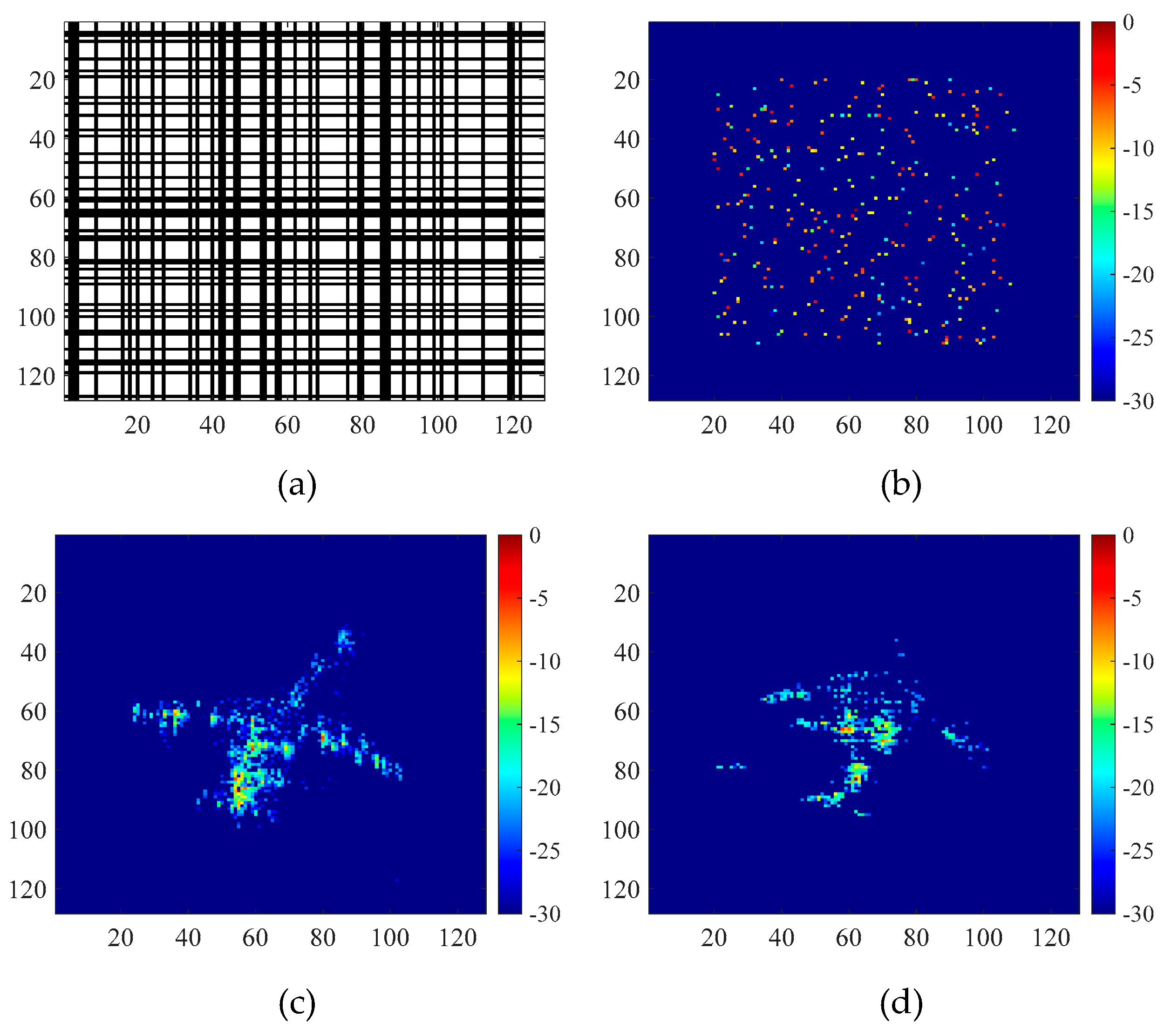
In this section, we will demonstrate the effectiveness of PAN with high-resolution imaging of 2D incomplete data. The missing data pattern of the 2D incomplete data is shown in Figure 3a, where the white bars denote the available data and the black ones denote the missing data, and the loss rate is 50%.

For network training, 1000 image pairs $\left(Y,X^{gt}\right)$ were generated as the simulated data set, where each $X^{gt}$ includes randomly distributed scattering centers with Gaussian amplitude. The training set consisted of 800 samples and the test set consisted of 200 samples. The SNR of the range-compressed echoes of the training set ranged from 2 dB to 20 dB; while the SNR of the range-compressed echoes of the test set was set to 5 dB, 10 dB, and 15 dB, respectively. The label image of a typical noise-free test sample is shown in Figure 3b.

To evaluate the imaging and generalization performance of PAN on measured data, two additional test sets of airplanes were selected. For complete data and high SNR, their RD images are shown in Figure 3c and Figure 3d. Then, the SNR of the range-compressed echoes was set to 5 dB, 10 dB, and 15 dB, respectively, by adding Gaussian noise.

As a comparison, we provide imaging results of the 2D-ADN [16], UNet [19], and PnP 2D ADMM, respectively. According to the analysis given in Section 1, we needed to build a model set for the noise-level dependent, model-driven 2D-ADN, as the SNR is varying among echoes. Therefore, we trained three 2D-ADNs for SNRs of 5 dB, 10 dB, and 15 dB, respectively.

For quantitative performance evaluation, we calculated the normalized mean square error (NMSE), the peak signal-to-noise ratio (PSNR), the structure similarity index measure (SSIM), entropy (ENT), and the running time.

The computing platform was an Intel i9-10920X 3.50-GHz computer with a 12-core processor and 64 GB RAM. In addition, UNet, PnP 2D ADMM and PAN were implemented on an NVIDIA GTX3090 GPU with 24 GB RAM using the framework of Pytorch. The 2D-ADN was implemented on a CPU within the framework of MATLAB.

5.1. 2D Incomplete Data

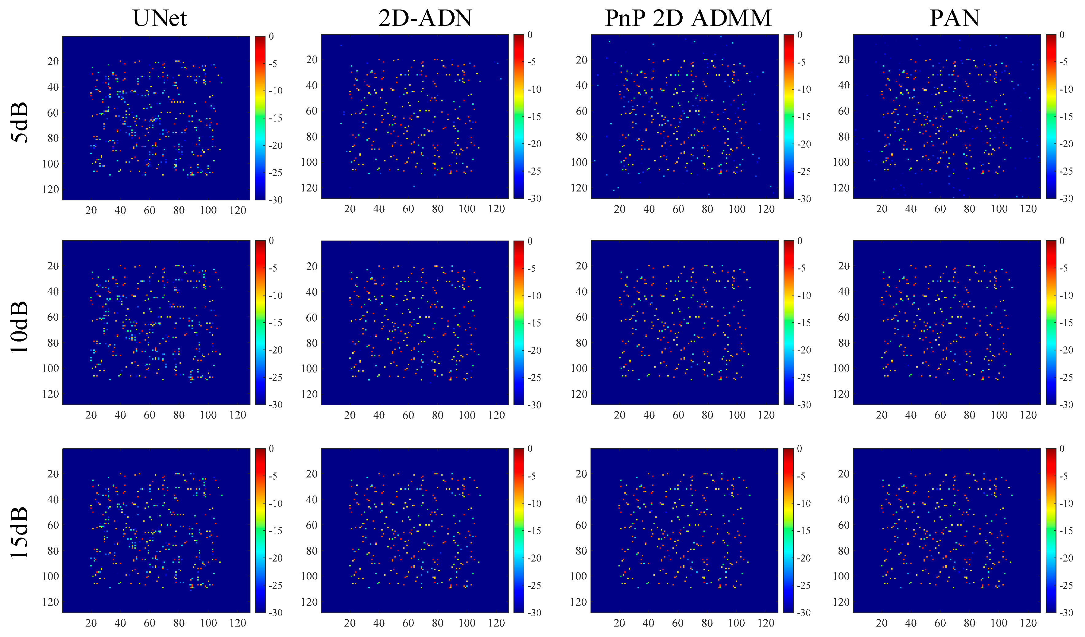
For the test data illustrated in Figure 3b, the imaging results are shown in Figure 4, and for the test set, the average metrics of the 200 samples with SNR of 5 dB, 10 dB, and 15 dB are shown in Table 1,

Table 2. Performance evaluation for the simulated 2D incomplete data under 10 dB condition.

Method	NMSE	PSNR	SSIM	Time(s)
UNet	0.4348	41.5182	0.9648	0.01
2D-ADN	0.0902	55.1677	0.9972	0.09
PnP 2D ADMM	0.1209	52.4912	0.9934	0.96
PAN	0.1104	53.4170	0.9957	0.01

and

Table 3. Performance evaluation for the simulated 2D incomplete data under 15 dB condition.

Method	NMSE	PSNR	SSIM	Time(s)
UNet	0.4243	41.7323	0.9671	0.01
2D-ADN	0.0522	59.9237	0.9991	0.09
PnP 2D ADMM	0.0945	55.0804	0.9966	1.24
PAN	0.0872	55.4826	0.9973	0.01

, respectively. It can be observed that the data-driven model, i.e., the UNet, gives unsatisfying imaging results on incomplete 2D data, due to the lack of theoretical support and sparse constraints. On the contrary, the rest of the methods were based on the 2D ADMM and demonstrated better reconstruction performance on the incomplete data.

In addition, the parameters of the different methods are shown in

Table 4. Parameters of different methods.

Method	UNet	2D-ADN	PnP 2D ADMM	PAN
Parameter No.	7.7M	41	0.04M	0.11M

, although parameters of PAN are 1/70 of the UNet, it is observed that PAN had the highest PSNR, SSIM, and the smallest NMSE (except for 2D-ADN with single SNR), demonstrating its superior imaging performance and robustness to different noise levels. In addition, we adjusted the penalty parameters of PnP 2D ADMM manually to obtain better imaging results, which led to a low efficiency. The PnP 2D ADMM had the longest running time, as more iterations were required to obtain well-focused imaging results.

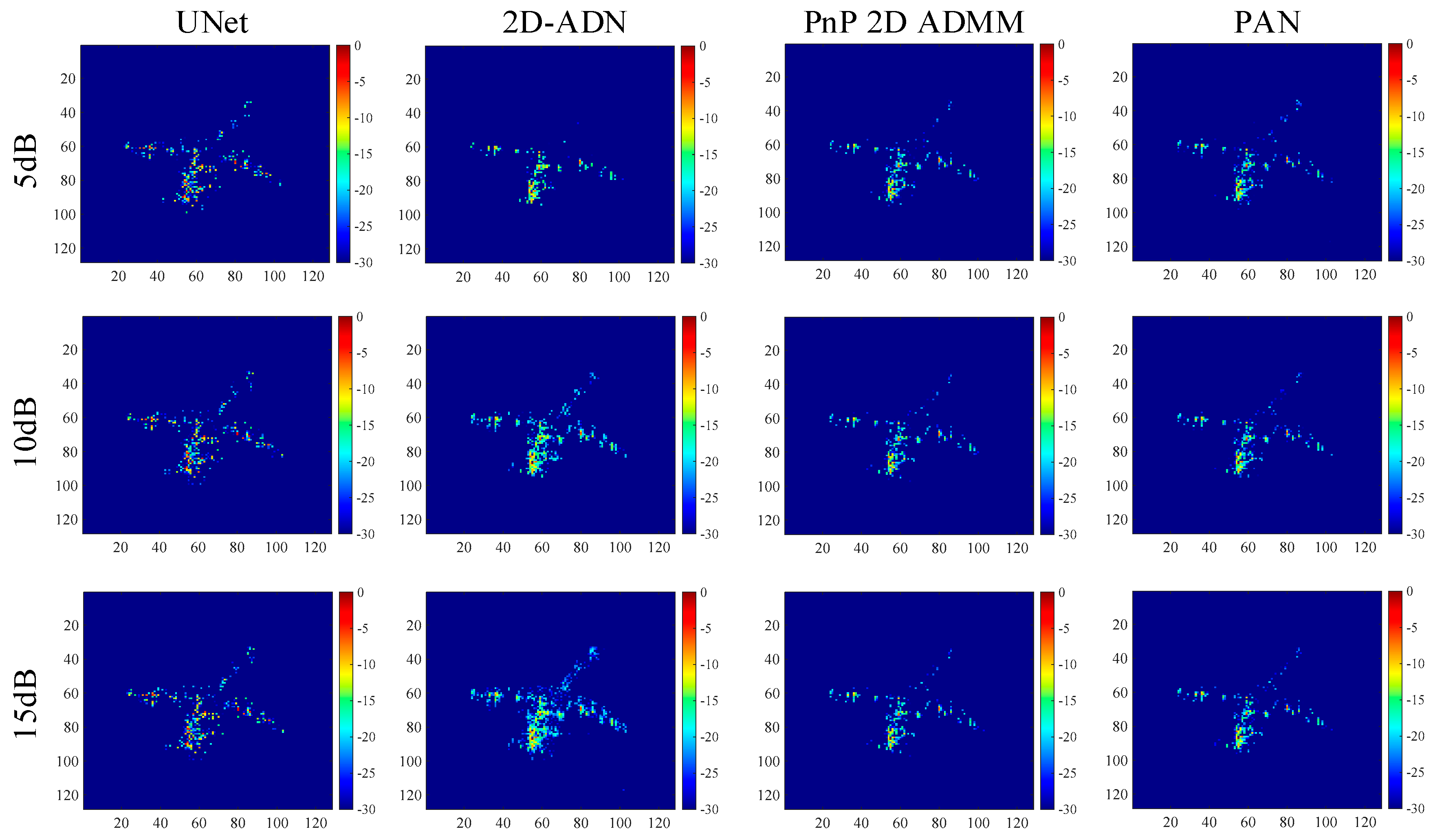
For the measured data illustrated in Figure 3c, the imaging results are shown in Figure 5, and the corresponding entropy (ENT) and running time are shown in

Table 5. Performance evaluation for the measured 2D incomplete data under different SNR conditions.

	5 dB		10 dB		15 dB
	ENT	Time(s)	ENT	Time(s)	ENT	Time(s)
UNet	0.7613	0.01	0.7809	0.01	0.7880	0.01
2D-ADN	0.5543	0.09	1.1620	0.09	1.4854	0.09
PnP 2D ADMM	0.4938	1.16	0.4753	1.47	0.4754	1.93
PAN	1.4245	0.01	1.3236	0.01	1.3063	0.01

. It is observed that although 2D-ADN had a lower entropy in low SNR scenarios, it had a poor generalization performance, as shown in Figure 5. On the contrary, PAN had a more complete structure, demonstrating its superior reconstruction performance on the measured data. In addition, UNet had artifacts, demonstrating its poor generalization performance.

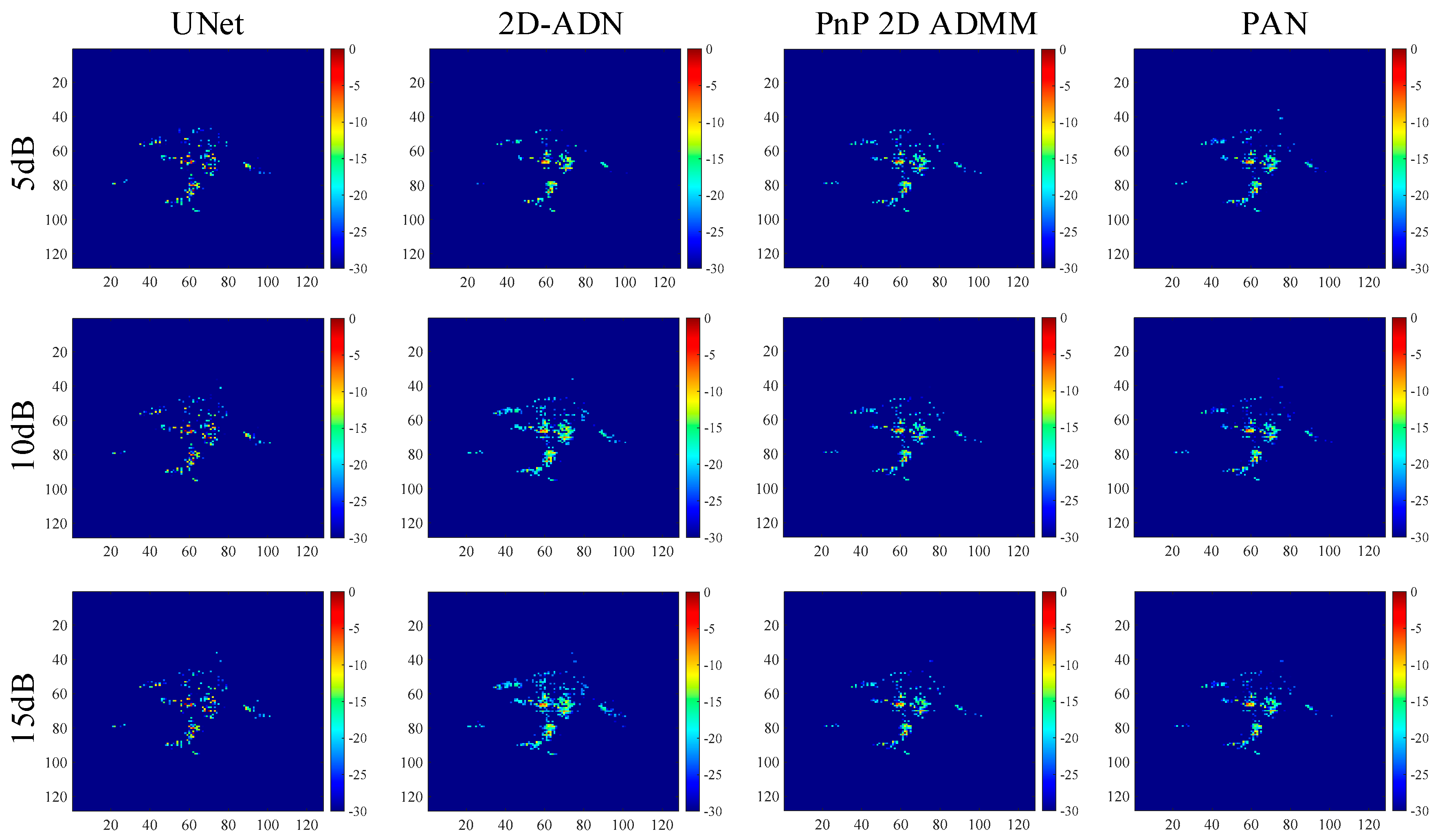
For another set of measured data, illustrated in Figure 3d, the imaging results are shown in Figure 6, and the corresponding entropy and running time are listed in

Table 6. Performance evaluation for another measured 2D incomplete dataset under different SNR conditions.

	5 dB		10 dB		15 dB
	ENT	Time(s)	ENT	Time(s)	ENT	Time(s)
UNet	0.5918	0.01	0.5969	0.01	0.5969	0.01
2D-ADN	0.4115	0.09	0.7905	0.09	0.6836	0.09
PnP 2D ADMM	0.3854	1.18	0.3820	1.71	0.3763	1.82
PAN	1.0400	0.01	0.9465	0.01	0.9319	0.01

. It can be seen that PAN had the best imaging results, indicating its good generalization performance on the measured data.

5.2. Different Loss Rates

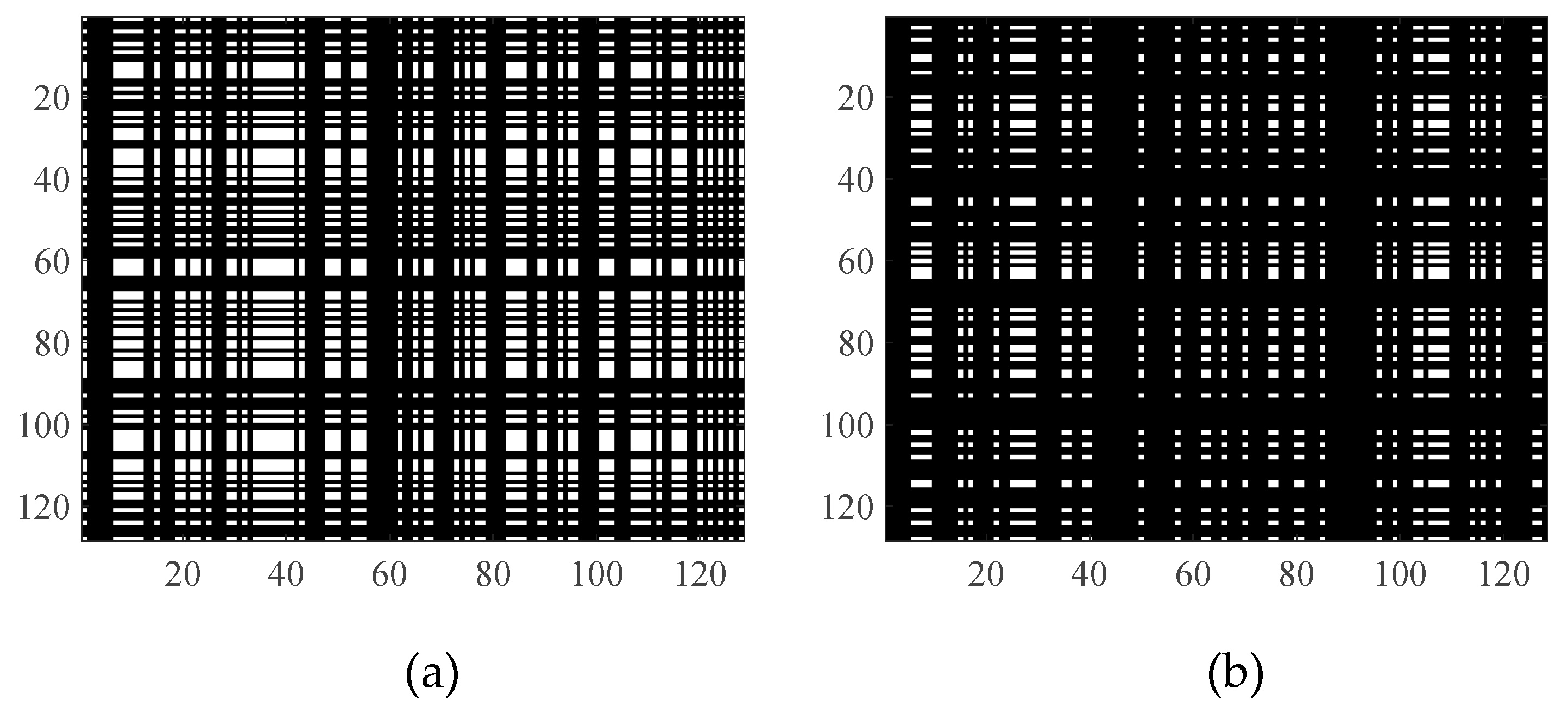
In order to further analyze the imaging performance of PAN with different loss rates, we designed more experiments with only 25% and 10% available data, the data missing patterns of a 75% loss rate and 90% loss rate are shown in Figure 7a and Figure 7b, respectively.

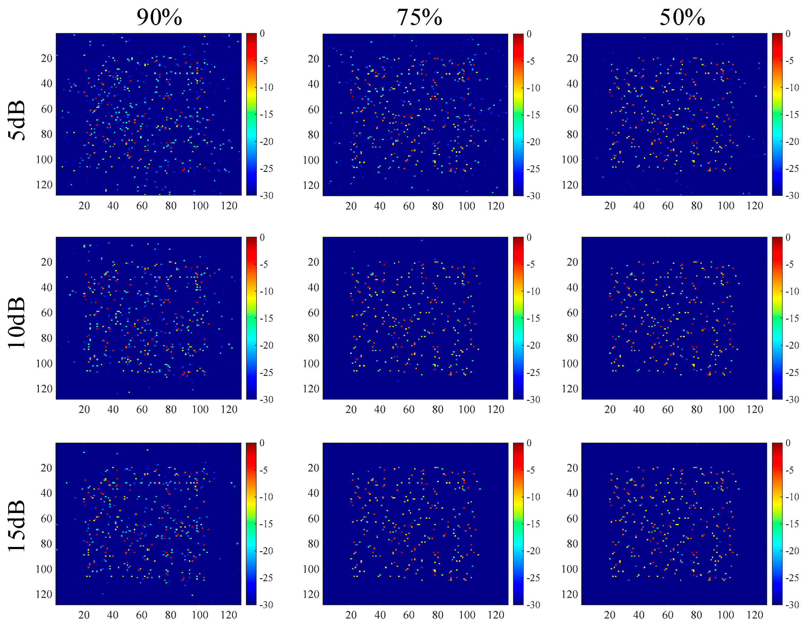
For the test data illustrated in Figure 3b, the imaging results are shown in Figure 8, and for the test set, the average metrics of the 200 samples with SNRs of 5 dB, 10 dB, and 15 dB are shown in

Table 7. Performance evaluation for the simulated data with different loss rates under the 5 dB condition.

Method	NMSE	PSNR	SSIM	Time(s)
50%	0.2035	48.1073	0.9847	0.01
75%	0.3371	43.7168	0.9612	0.01
90%	0.6817	37.5979	0.8779	0.01

,

Table 8. Performance evaluation for the simulated data with different loss rates under the 10 dB condition.

Loss Rate	NMSE	PSNR	SSIM	Time(s)
50%	0.1104	53.4170	0.9957	0.01
75%	0.2066	47.9707	0.9856	0.01
90%	0.5814	38.9823	0.9077	0.01

, and

Table 9. Performance evaluation for the simulated data with different loss rates under the 15 dB condition.

Loss Rate	NMSE	PSNR	SSIM	Time(s)
50%	0.0872	55.4826	0.9973	0.01
75%	0.1717	49.5959	0.9900	0.01
90%	0.5423	39.5876	0.9186	0.01

, respectively. It is observed that the test data with 90% loss rate had the worst imaging result under a 5 dB SNR. However, when we raised the SNR to 10 dB or 15 dB, the imaging performance improved rapidly. In addition, if we reduced the loss rate to 75% or 50%, the imaging performance also improved rapidly.

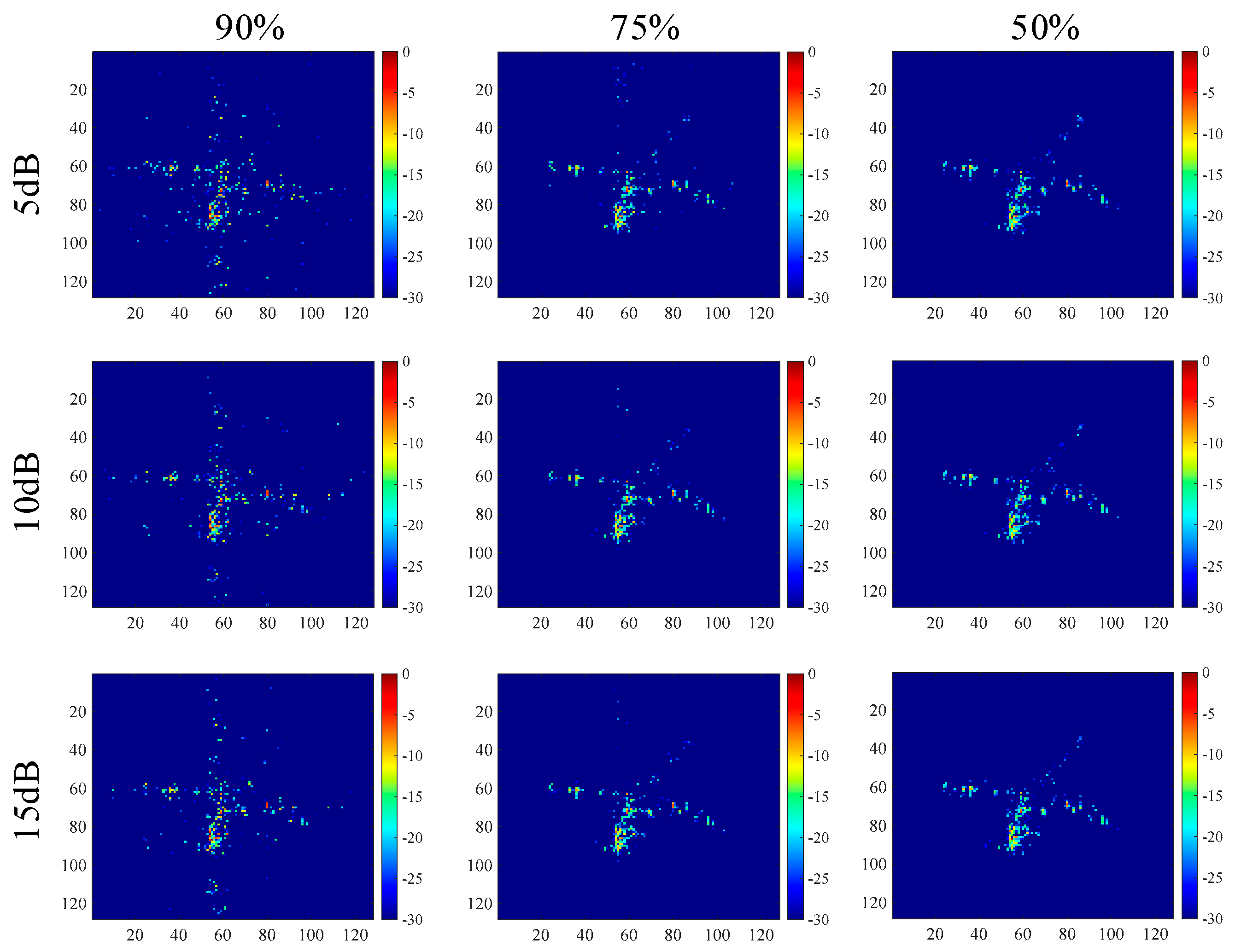
For the measured data illustrated in Figure 3c, the imaging results are shown in Figure 9, and the corresponding entropy (ENT) and running time are shown in

Table 10. Performance evaluation for the measured data with different loss rates under different SNR conditions.

	5 dB		10 dB		15 dB
	ENT	Time(s)	ENT	Time(s)	ENT	Time(s)
50%	1.4245	0.01	1.3236	0.01	1.3063	0.01
75%	1.5640	0.01	1.4885	0.01	1.4854	0.01
90%	1.9654	0.01	1.8782	0.01	1.8522	0.01

. It is observed that the test data with 90% loss rate had a lot of false points and artifacts. However, if we reduced the loss rate to 75% or 50%, the imaging performance improved rapidly.

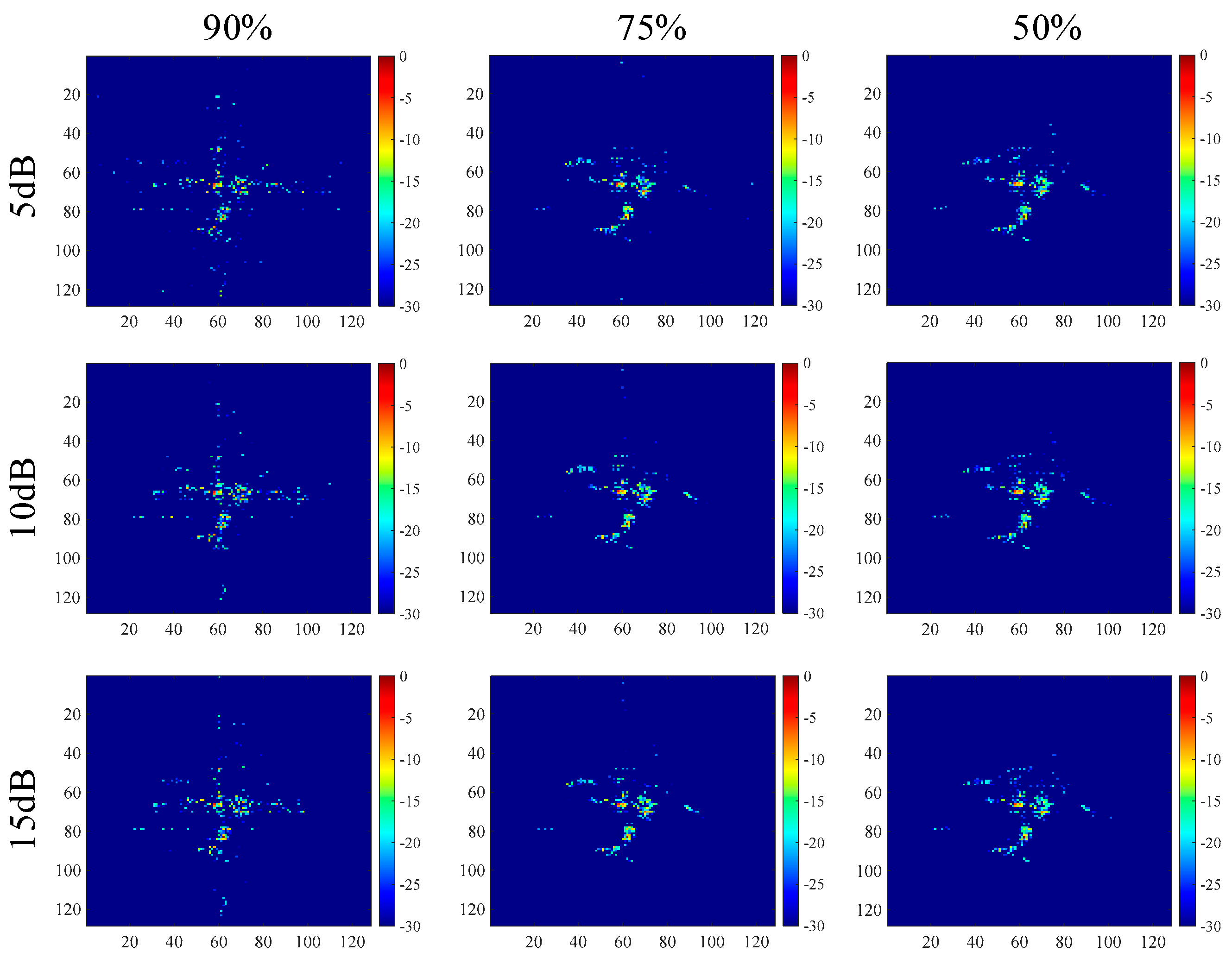
For another measured dataset, illustrated in Figure 3d, the imaging results are shown in Figure 10, and the corresponding entropy and running time are listed in

Table 11. Performance evaluation for another measured dataset with different loss rate under different SNR conditions.

	5 dB		10 dB		15 dB
	ENT	Time(s)	ENT	Time(s)	ENT	Time(s)
50%	1.0400	0.01	0.9465	0.01	0.9319	0.01
75%	1.4168	0.01	1.4174	0.01	1.4264	0.01
90%	1.8238	0.01	1.7711	0.01	1.7366	0.01

. The test data with a 75% loss rate had a better imaging result than the test data with 90% loss rate, demonstrating that the loss rate had a significant impact on the imaging performance.

6. Discussion

To obtain the optimal imaging results, it is necessary to design the structure of PAN in two aspects: (a) the number of stages; and (b) the depth of DnCNN. The discussions below are based on the simulated data presented in Section 5.

6.1. The Number of Stages

For PAN, the number of stages corresponds to the number of iterations in PnP 2D ADMM. As the stage number increases, the runtime becomes longer.

Table 12. Parameters of different stages.

Stage No.	3	4	5	6	7	8
Parameter No.	0.08M	0.11M	0.15M	0.19M	0.23M	0.27M

presents the number of parameters for different stages, and Figure 11 shows the variation of NMSE, PSNR, and SSIM with the number of stages. It is observed that the curve is relatively stable; thus, we set the stage number to 4 in the experiments to reduce the model complexity.

6.2. The Depth of DnCNN

As a denoising layer in PAN, the DnCNN has the most adjustable parameters. When the number of stages is fixed to 4, the number of parameters for different depths are shown in

Table 13. Parameters of different depth.

Stage No.	2	3	4	5	6	7
Parameter No.	3658	0.11M	0.23M	0.34M	0.45M	0.56M

. It is observed that compared with the stage number, the depth of DnCNN has a larger impact on the number of parameters. Figure 12 shows the variation of NMSE, PSNR, and SSIM with the network depth, where the reconstruction performance is stable when the depth of DnCNN is larger than 3.

7. Conclusions

This article proposed a PAN for sparse ISAR imaging of 2D incomplete data with various SNRs. First, PnP 2D ADMM was proposed for 2D ISAR imaging by combining a data-driven deep network DnCNN and sparse signal reconstruction method 2D ADMM. On this basis, the PnP 2D ADMM was generalized and unrolled into PAN, which had robustness to noise and satisfying reconstruction performance for incomplete data. Experiments demonstrated that, compared with the available methods, PAN with a single parameter set could achieve better-focused imaging with a higher computational efficiency for measured data under various SNRs.

To deal with the open problem of optimal parameter selection, future work will be focused on presenting tuning-free algorithms that can determine parameters automatically based on a deep network.

References

1. Luo, Y.; Zhang, Q.; Yuan, N.; Zhu, F.; Gu, F. Three-dimensional precession feature extraction of space targets. IEEE Trans. Aerosp. Electron. Syst. 2014, 50, 1313–1329. [Google Scholar] [CrossRef]
2. Bai, X.R.; Zhou, X.N.; Zhang, F.; Wang, L.; Zhou, F. Robust pol-ISAR target recognition based on ST-MC-DCNN. IEEE Trans. Geosci. Remote Sens. 2019, 57, 9912–9927. [Google Scholar] [CrossRef]
3. Carrara, W.G.; Goodman, R.S.; Majewski, R.M. Spotlight Synthetic Aperture Radar: Signal Processing Algorithms; Artech House: Boston, MA, USA, 1995; Chapter 2. [Google Scholar]
4. Wang, D.; Zhang, Q.; Luo, Y.; Liu, X.; Ni, J.; Su, L. Joint optimization of time and aperture resource allocation strategy for multi-target ISAR Imaging in radar sensor network. IEEE Sens. J. 2021, 21, 19570–19581. [Google Scholar] [CrossRef]
5. Zhao, L.F.; Wang, L.; Yang, L.; Zoubir, A.M.; Bi, G.A. The race to improve radar imagery: An overview of recent progress in statistical sparsity-based techniques. IEEE Signal Process. Mag. 2016, 33, 85–102. [Google Scholar] [CrossRef]
6. Kang, L.; Luo, Y.; Zhang, Q.; Liu, X.W.; Liang, B.S. 3-D Scattering Image Sparse Reconstruction via Radar Network. IEEE Trans. Geosci. Remote Sens. 2022, 60, 1–14. [Google Scholar] [CrossRef]
7. Kang, M.; Lee, S.; Lee, S.; Kim, K. ISAR imaging of high-speed maneuvering target using gapped stepped-frequency waveform and compressive sensing. IEEE Trans. Image Process. 2017, 26, 5043–5056. [Google Scholar] [CrossRef]
8. Hu, P.J.; Xu, S.Y.; Wu, W.Z.; Chen, Z.P. Sparse subband ISAR imaging based on autoregressive model and smoothed 0 algorithm. IEEE Sens. J. 2018, 18, 9315–9323. [Google Scholar] [CrossRef]
9. Li, S.; Amin, M.; Zhao, G.; Sun, H. Radar imaging by sparse optimization incorporating MRF clustering prior. IEEE Geosci. Remote Sens. Lett. 2020, 17, 1139–1143. [Google Scholar] [CrossRef] [Green Version]
10. Bai, X.R.; Zhou, F.; Hui, Y. Obtaining JTF-signature of space-debris from incomplete and phase-corrupted data. IEEE Trans. Aerosp. Electron. Syst. 2017, 53, 1169–1180. [Google Scholar] [CrossRef]
11. Qiu, W.; Zhao, H.; Zhou, J.; Fu, Q. High-resolution fully polarimetric ISAR imaging based on compressive sensing. IEEE Trans. Geosci. Remote Sens. 2014, 52, 6119–6131. [Google Scholar] [CrossRef]
12. Liu, Z.; Liao, X.; Wu, J. Image Reconstruction for Low-Oversampled Staggered SAR via HDM-FISTA. IEEE Trans. Geosci. Remote Sens. 2022, 60, 1–14. [Google Scholar] [CrossRef]
13. Hashempour, H.R. Sparsity-Driven ISAR Imaging Based on Two-Dimensional ADMM. IEEE Sens. J. 2020, 20, 13349–13356. [Google Scholar] [CrossRef]
14. Monga, V.; Li, Y.; Eldar, Y.C. Algorithm Unrolling: Interpretable, Efficient Deep Learning for Signal and Image Processing. IEEE Signal Process. Mag. 2021, 38, 18–44. [Google Scholar] [CrossRef]
15. Wei, S.; Liang, J.; Wang, M.; Shi, J.; Zhang, X.; Ran, J. AF-AMPNet: A Deep Learning Approach for Sparse Aperture ISAR Imaging and Autofocusing. IEEE Trans. Geosci. Remote Sens. 2022, 60, 1–14. [Google Scholar] [CrossRef]
16. Li, X.; Bai, X.; Zhou, F. High-resolution ISAR imaging and autofocusing via 2D-ADMM-Net. Remote Sens. 2021, 13, 2326. [Google Scholar] [CrossRef]
17. Wei, S.; Liang, J.; Wang, M.; Zeng, X.F.; Shi, J.; Zhang, X.L. CIST: An improved ISAR imaging method using convolution neural network. Remote Sens. 2020, 12, 2641. [Google Scholar] [CrossRef]
18. Hu, C.; Wang, L.; Li, Z.; Zhu, D. Inverse synthetic aperture radar imaging using a fully convolutional neural Network. IEEE Geosci. Remote Sens. Lett. 2020, 17, 1203–1207. [Google Scholar] [CrossRef]
19. Yang, T.; Shi, H.Y.; Lang, M.Y.; Guo, J.W. ISAR imaging enhancement: Exploiting deep convolutional neural network for signal reconstruction. Int. J. Remote Sens. 2020, 41, 9447–9468. [Google Scholar] [CrossRef]
20. Venkatakrishnan, S.V.; Bouman, C.A.; Wohlberg, B. Plug-and-Play Priors for Model Based Reconstruction. In Proceedings of the IEEE Global Conference on Signal and Information Processing (Global SIP), Austin, TX, USA, 3–5 December 2013; pp. 945–948. [Google Scholar]
21. Wei, K.; Avilés-Rivero, A.I.; Liang, J.; Fu, Y.; Schönlieb, C.; Huang, H. Tuning-free plug-and-play proximal algorithm for inverse imaging problems. In Proceedings of the 37th International Conference on Machine Learning, Vienna, Austria, 13–18 July 2020; pp. 10158–10169. [Google Scholar]
22. Dabov, K.; Foi, A.; Katkovnik, V.; Egiazarian, K. Image denoising by sparse 3D transform-domain collaborative filtering. IEEE Trans. Image Process. 2007, 16, 2080–2095. [Google Scholar] [CrossRef]
23. Zhang, K.; Zuo, W.; Chen, Y.; Meng, D.; Zhang, L. Beyond a Gaussian Denoiser: Residual Learning of Deep CNN for Image Denoising. IEEE Trans. Image Process. 2017, 26, 3142–3155. [Google Scholar] [CrossRef] [Green Version]
24. Dong, W.; Wang, P.; Yin, W.; Shi, G. Denoising Prior Driven Deep Neural Network for Image Restoration. IEEE Trans. Pattern Anal. Mach. Intell. 2018, 41, 2305–2318. [Google Scholar] [CrossRef] [PubMed] [Green Version]
25. Ahmad, R.; Bouman, C.A.; Buzzard, G.T.; Chan, S.; Liu, S.; Reehorst, E.T.; Schnitter, P. Plug-and-Play Methods for Magnetic Resonance Imaging: Using Denoisers for Image Recovery. IEEE Signal Process. Mag. 2020, 37, 105–116. [Google Scholar] [CrossRef] [PubMed] [Green Version]
26. He, J.; Yang, Y.; Wang, Y.; Zeng, D.; Bian, Z.; Zhang, H.; Sun, J.; Xu, Z.; Ma, J. Optimizing a Parameterized Plug-and-Play ADMM for Iterative Low-Dose CT Reconstruction. IEEE Trans. Med. Imaging. 2019, 38, 371–382. [Google Scholar] [CrossRef] [PubMed]
27. Ryu, E.K.; Liu, J.; Wang, S.; Chen, X.; Wang, Z.; Yin, W. Plug-and-play methods provably converge with properly trained denoisers. arXiv 2019, arXiv:1905.05406. [Google Scholar]
28. Kingma, D.P.; Ba, J. Adam: A method for stochastic optimization. arXiv 2014, arXiv:1412.6980. [Google Scholar]
Figure 1. Structure of the PAN.
Remotesensing 14 00901 g001
Figure 2. Structure of the denoising layer.
Remotesensing 14 00901 g002
Figure 3. Data set illustration. (a) Data missing pattern of the 2D incomplete data. (b) Label image of a test sample. (c) RD image of the measured data with complete data and high SNR. (d) RD image of another measured dataset with complete data and high SNR.
Remotesensing 14 00901 g003
Figure 4. ISAR images of Figure 3b with different SNR.
Remotesensing 14 00901 g004
Figure 5. ISAR images of measured data with different SNRs.
Remotesensing 14 00901 g005
Figure 6. ISAR images of another measured dataset with different SNRs.
Remotesensing 14 00901 g006
Figure 7. The missing data pattern of (a) 75% loss rate and (b) 90% loss rate.
Remotesensing 14 00901 g007
Figure 8. ISAR images of Figure 3b with different loss rates and different SNRs.
Remotesensing 14 00901 g008
Figure 9. ISAR images of measured data with different loss rates and different SNRs.
Remotesensing 14 00901 g009
Figure 10. ISAR images of another measured dataset with different loss rates and different SNRs.
Remotesensing 14 00901 g010
Figure 11. Variation of (a) NMSE, (b) PSNR, and (c) SSIM with the number of stages.
Remotesensing 14 00901 g011
Figure 12. Variation of (a) NMSE, (b) PSNR, and (c) SSIM with the number of layers for DnCNN.
Remotesensing 14 00901 g012