Abstract
Computer vision for large scale building detection can be very challenging in many environments and settings even with recent advances in deep learning technologies. Even more challenging is modeling to detect the presence of specific buildings (in this case schools) in satellite imagery at a global scale. However, despite the variation in school building structures from rural to urban areas and from country to country, many school buildings have identifiable overhead signatures that make them possible to be detected from high-resolution imagery with modern deep learning techniques. Our hypothesis is that a Deep Convolutional Neural Network (CNN) could be trained for successful mapping of school locations at a regional or global scale from high-resolution satellite imagery. One of the key objectives of this work is to explore the possibility of having a scalable model that can be used to map schools across the globe. In this work, we developed AI-assisted rapid school location mapping models in eight countries in Asia, Africa, and South America. The results show that regional models outperform country-specific models and the global model. This indicates that the regional model took the advantage of having been exposed to diverse school location structure and features and generalized better, however, the global model was the worst performer due to the difficulty of generalizing the significant variability of school location features across different countries from different regions.
1. Introduction
Reliable and accurate data about school locations have become vital to many humanitarian agencies and governments to effectively plan, manage, and monitor the provision of quality education and learning in accordance to the UN sustainable development goal 4 (SDG4 [1]) that ensure equal access to opportunity (SDG10 [1]) [2]. For example, UNICEF and ITU (International Telecommunication Union) launched a program named Giga [3] which is a global initiative to connect every school in the world to the internet and every student to information, opportunity, and choice by 2030. Lack of internet connectivity does not just limit students’ ability to connect online, it prevents and isolates them from competing in the modern economy. Connecting schools to the internet starts by mapping the locations and other attributes of these schools. In addition, understanding the location of schools can help governments and international organizations gain critical insights into the needs of vulnerable populations, and better prepare and respond to exogenous shocks such as disease outbreaks or natural disaster development programs aiming to provide internet connection to schools in developing countries which requires accurate and comprehensive datasets of school locations [2]. However, in many countries, data about educational facilities is often inaccurate, incomplete, outdated, or even non-existent. Open data sources such as the OpenStreetMap (OSM) have been very useful for many large-scale land use mapping projects including school locations [4,5], however, we have discovered sparse and even no coverage of OSM school location data in many developing countries of our interest. Some of the available OSM data points formed part of our training dataset as described in Table 1.

Table 1.
School data sources for this study from UNICEF Office of Innovation and OpenStreetMap (OSM). Before and after training dataset validation.
A recent study demonstrated that Deep Neural Network (DNN)-based models can deliver high accuracy and precision in identifying school buildings from high resolution satellite imagery [6]. Studies have shown that humans can be trained to identify school buildings in high resolution image tiles, and they do that effectively with over 90% accuracy, however, to do this at a global scale is unrealistic.
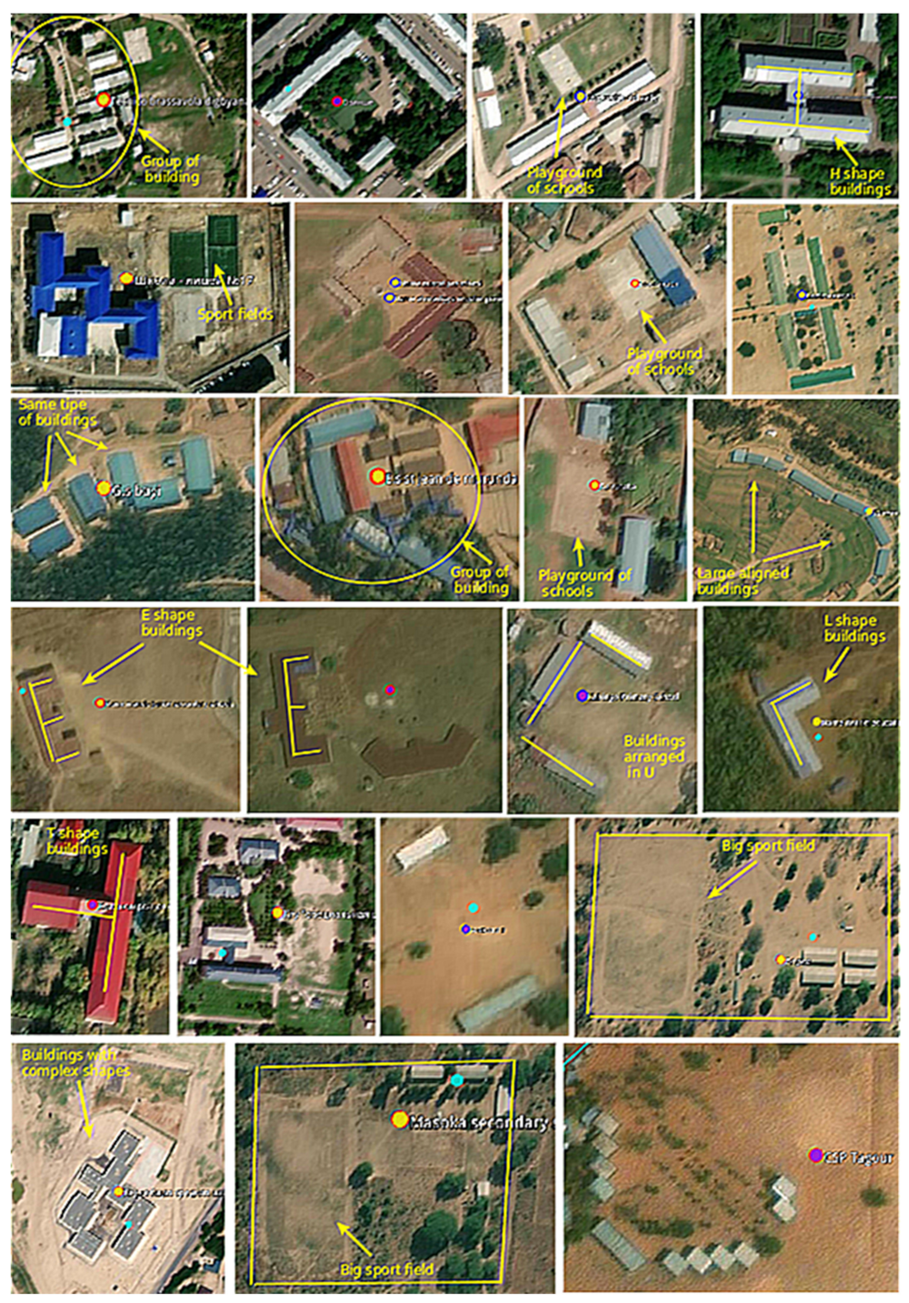
Despite the varying structure of school location features, many school structures have identifiable overhead signatures that make them detectable in high-resolution imagery with modern deep learning techniques. Some of the identifiable features from space include building size, shape, and facilities. Compared to the surrounding buildings, school structures are usually bigger in size, and the shapes vary from U, O, H, E, or L as shown in Figure 1.
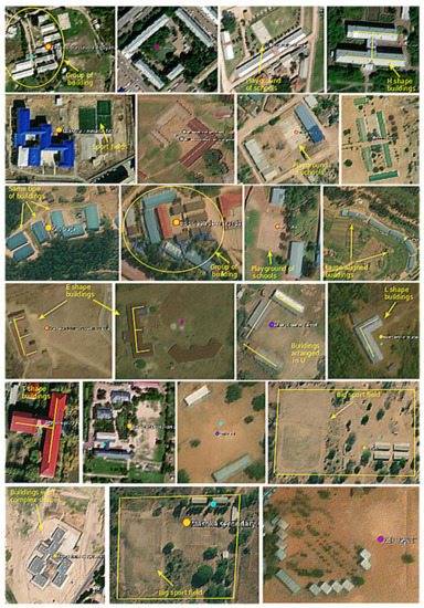
Figure 1.
School location structure showing identifiable signatures on overhead imagery.
This study aims at developing rapid and scalable Artificial Intelligence (AI) models that can deliver automated and swift mapping of schools using high resolution satellite imagery in eight different countries from Asia, Africa, and South America. To achieve this goal, we develop and test DNN models based on the Xception [7] and the MobileNetV2 [8] models modified for application on satellite imagery at country, regional, and global scales.
These models are tile-based classifiers based on high-performance and accurate binary classification Convolutional Neural Network (CNN). The models could scan through 71 million zoom 18 tiles (256 × 256 pixels per tile in 60 cm meter high-resolution Maxar Vivid imagery) and identify schools in near real-time. This study developed and tested six specific country models that were tuned to perform well within the country’s territorial boundaries, two regional models, and a global model. The two regional models were the East African model that was trained with school location data from Kenya and Rwanda, and the West African model that was trained with datasets from Sierra Leone and Niger. The global models were trained with all countries’ school datasets. Both regional and global models were trained to generalize well in the geo-diverse landscape. By testing the East African regional and Kenya tile-based school classifier models in Kenya, we found the regional model outperformed the country-specific model. It indicates that the model that was exposed to diverse looks and school features can outperform the model that only trains with limited features.
In summary, there has recently been a lot of research on the use of DNN to identify and extract different objects and infrastructure from overhead satellite imagery [9,10], however, the applicability, generalizability, and scalability of deep learning techniques on overhead satellite imagery in the context of school mapping at scale especially in developing countries has not yet been explored which is indeed the gap that inspires this paper. The major contributions of this study are two-fold:
- The development of scalable deep learning models to automatically map school locations at global, regional, and country-level scales in near real-time considering the variability in school structure from rural to urban and from country to country. From our literature review, no study has been carried out in this area with the context of providing a contribution to the research communities and school infrastructure mapping at scale for humanitarian and open-source projects.
- Exploring the generalizability of deep learning models in the context of transfer learning of school features where a DNN model trained in a given geolocation can generalize to detect schools in another geolocation without been re-trained with new datasets.
2. Background
Deep Neural Networks (DNNs) have proven to be very effective compared to traditional approaches, particularly object extraction from overhead satellite imagery at scale and speed [11,12,13,14,15,16]. On the other hand, the traditional approaches for object detection depend majorly on manual extraction processes which are inefficient and inadequate for generalization requirements and computationally exhausting. For deep learning algorithms, visual perception to extract feature hierarchies and generalization ability is enhanced on several levels [12]. These algorithms have shown that traditional techniques are slow and erroneous; they require extensive post-processing to differentiate infrastructure [17]. However, automatic school detection and mapping from overhead imagery requires very advanced DNN classifiers that work beyond task-based methods for object recognition and can carry out adaptive and deep learning from multi-resolution imagery for object detection.
Methods utilizing DNNs are now deemed to be conventional for image segmentation [18,19,20] based on the wide adoption and many studies utilizing different DNN architecture for object detection such as in [21,22,23,24,25,26,27]. This is an evolving area, and new studies are frequently published on different approaches to deal with some of the shortcomings of DNNs. These include, for example, methods for evaluating biases in DNN for infrastructure mapping [6], the large computing and memory requirements [28], large training data requirement, difficulty in generalizing and adapting models to varying conditions [29], and so on. The U-Net DNN [30] architecture became very popular and the standard model for semantic segmentation in many applications won the IEEE International Symposium on Biomedical Imaging cell tracking challenge in 2015. The popularity of this DNN architecture stems from its contracting path for capturing context and the symmetric expanding path that enables precise localization, partly due to its speed, and its ability to be trained end-to-end with very few images [6]. Different variants of U–Net have been developed for different applications including for building and road detection [31,32,33,34]. However, new DNN architecture with greater speed and accuracy requiring less training images have emerged in recent times as described below.
Amongst the earliest works on object detection based on deep learning that achieved a mean Average Precision (mAP) of 98.7% with pre-trained AlexNet on a 1000 image set is the work of Zhao et al. [35].
One fundamental issue in school building detection using DNN is training data inadequacy because for DNN models to generalize efficiently, there is a large number of school structure variants to train on. Different approaches have been proposed in the literature to deal with deficiency in training samples such as in [36,37,38,39,40,41]. Other studies have explored the use of transfer learning and few-shot learning to boost training sample variation. Examples include Bai et al. [42] where they utilized the transfer learning technique on the ImageNet data kit, however, these studies dealt with items that have well defined structures, colors, shapes, and sizes such as insulator faults, road cracks, solar farms, etc., unlike school buildings that have varying structures, colors, sizes, and shapes.
One interesting approach for specific object detection from a group of objects is the two-step object detection technique. First is to identify, for example, buildings from non-buildings afterwards to detect the building structure of interest from a group of detected buildings. In view of this, Tao et al. [43] developed two separate backbone models for electricity transmission line fault detection, namely Defect Detector Network (DDN) and Insulator localizer Network (ILN) for insulator detection based on the Visual Geometry Group (VGG) model and Residual Network (ResNet) model. respectively. We explored this approach further in this study.
Convolutional Neural Networks (CNNs) have emerged as one of the most popular DNN architectures developed for 2D images. CNNs have become very popular for many deep learning tasks including image classification, object detection [21], and image segmentation, as well as edge detection [44]. The Deep CNN was initially utilized for image classification problems due to the capabilities of deep convolution layers to recognize edges, patterns, context, and shapes which gives rise to more features with spatial dimensions smaller and deeper than the original [45]. AlexNet feature extractor developed by Krizhevsky et al. [46] with an 8-layer CNN, 5 convolutional layers + 3 fully connected layers won the ImageNet challenge of 2012 and could be seen as the precursor to image classification architecture. Different variants of Krizhevsky et al. architecture have been developed over the years to improve the model based on narrower receptive windows and increasing the network depth.
The ImageNet challenge 2014 gave rise to the VGGNet deep learning network architecture which is deemed to be an improvement to the Krizhevsky et al. model. The VGG won the challenge in the object localization task and gained second place in the classification task [47]. Convolutional network has achieved high performance accuracy in image classification and object identification through the gradient-based learning process, especially through the use loss computation and the loss function [42]. The complexity in image classification problems such as in this case study of school building detection increasingly calls for deeper CNNs. However, deeper CNNs with tens of layers can be difficult to train because of the problem of vanishing and exploding gradients. To deal with this problem of exploding and vanishing gradients, the residual network architecture called the ResNet started to gain attention. Residual network architecture is designed based on the skipping concept to the VGG networks [48]. ResNet proposes a shallower network depth using shortcut connections, directly connecting the early layer’s input to a later layer. This creates a significant capability to train very deep CNNs of up to 50, 101, and 152 layers with improved speed [49], thanks to the regular cut-off’s connection (skipping) among the Deep CNN blocks.
Based on these CNN performances in image classification and the necessity to utilize the method for more complex image classification problems such as in this case study, the object detection variant of the CNN was developed [21]. The Faster R-CNN came to light as a region-based CNN for discrete object detection. Faster R-CNN carries out object detection based on two modules: the Regional Proposal Network (RPN) for detecting regions, and the Region-CNN (R-CNN) detector for classifying regions and refining bounding boxes [50,51]. This DNN architecture utilizes the CNN model pretrained for classification to generate the necessary activation feature map [52]. Afterwards, the extracted feature maps are passed through the RPN to generate the object proposal [21]. Each object proposal is then employed by the network to generate the fixed feature maps of objects of interest. Thereafter, the final Region-based CNNs (R-CNN) combines the prior output and the class details based on region proposals. Utilizing the object proposals extracted through RPN as well as the extracted features of the proposals (via ROI pooling), the final class and object localization is accomplished [53]. Although faster R-CNN is exceptionally reliable, it appears to be slower in training speed when compared with MobileNet.
For real-time object detection purposes which requires a balance between time, speed, and accuracy, many multiple single-phase DNN architectures have been developed which includes MobileNet [8], the ‘You Only Look Once’ (YOLO) [54] and Single-shot detector (SSD) [55] frameworks.
There have recently been several alterations to the SSD framework which has resulted in its better performance than the YOLO. Some of these changes include the prediction of multi-feature maps from the subsequent networking stage to allow multiscale detection prediction of object classes and offsets at bounding box locations using smaller convolutional filters, and generating the final feature map by using different predictors to identify objects at varying aspect ratios in the form of feature pyramids [56].
For low-latency applications such as for mobile and embedded systems, Howard [8] developed a lightweight deep neural network model referred to as Mobile Networks (MobileNets). MobileNets and its derivatives have been developed to improve speed constraint associated with deeper networks for real-time applications. This idea is that the regular neural network convolution layer is broken down into two filters, depth-wise convolution and pointwise convolution. The conventional convolutional filter is more computationally expensive when compared to the depth-wise and point-wise convolutions. In MobileNets, each channel is convolved with its kernel, called a depth-wise convolution. Afterwards, the pointwise (1 × 1) convolution is processed to abstract and integrate the individual intermediate output from the depth-wise convolution into a single feature layer.
In view of this, we utilized the ResNet152 and SSD MobileNet in this study for school building detection and the Xception CNN for tile-based school image classification. These are, relatively, the most suitable models based on our approach and objectives. This Xception [57] architecture has 36 convolutional layers forming the feature extraction base of the network. In this architecture, cross-channel correlations and spatial correlations in the feature maps of convolutional neural networks can be entirely decoupled. The 36 convolutional layers are structured into 14 modules, all of which have linear residual connections around them, except for the first and last modules. In other words, the Xception architecture is a linear stack of depth-wise separable convolution layers with residual connections which makes it relatively faster to train. The Xception architecture is easier to define and modify as it takes only few lines of code based on the high-level library called Keras [58].
3. Materials and Methods
This section outlines the workflow and methods utilized for model training and development at scale. It also provides a description of the algorithm architecture and components.
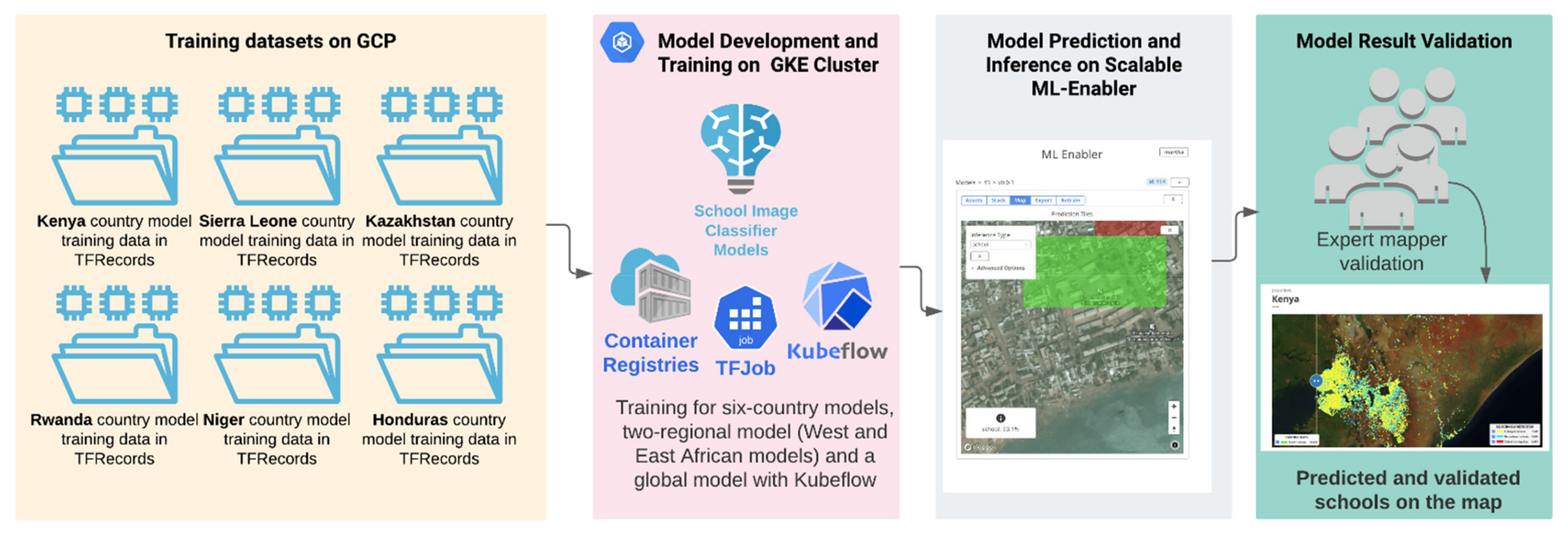
Figure 2 describes the workflow design for scalable development and deployment of the school classifier models. The school classifier models are developed based on the Xception deep learning backbone whose architecture is described in Figure 3.
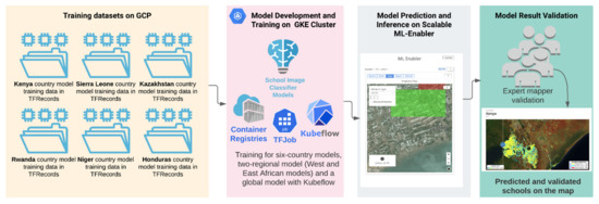
Figure 2.
Model development and deployment workflow.

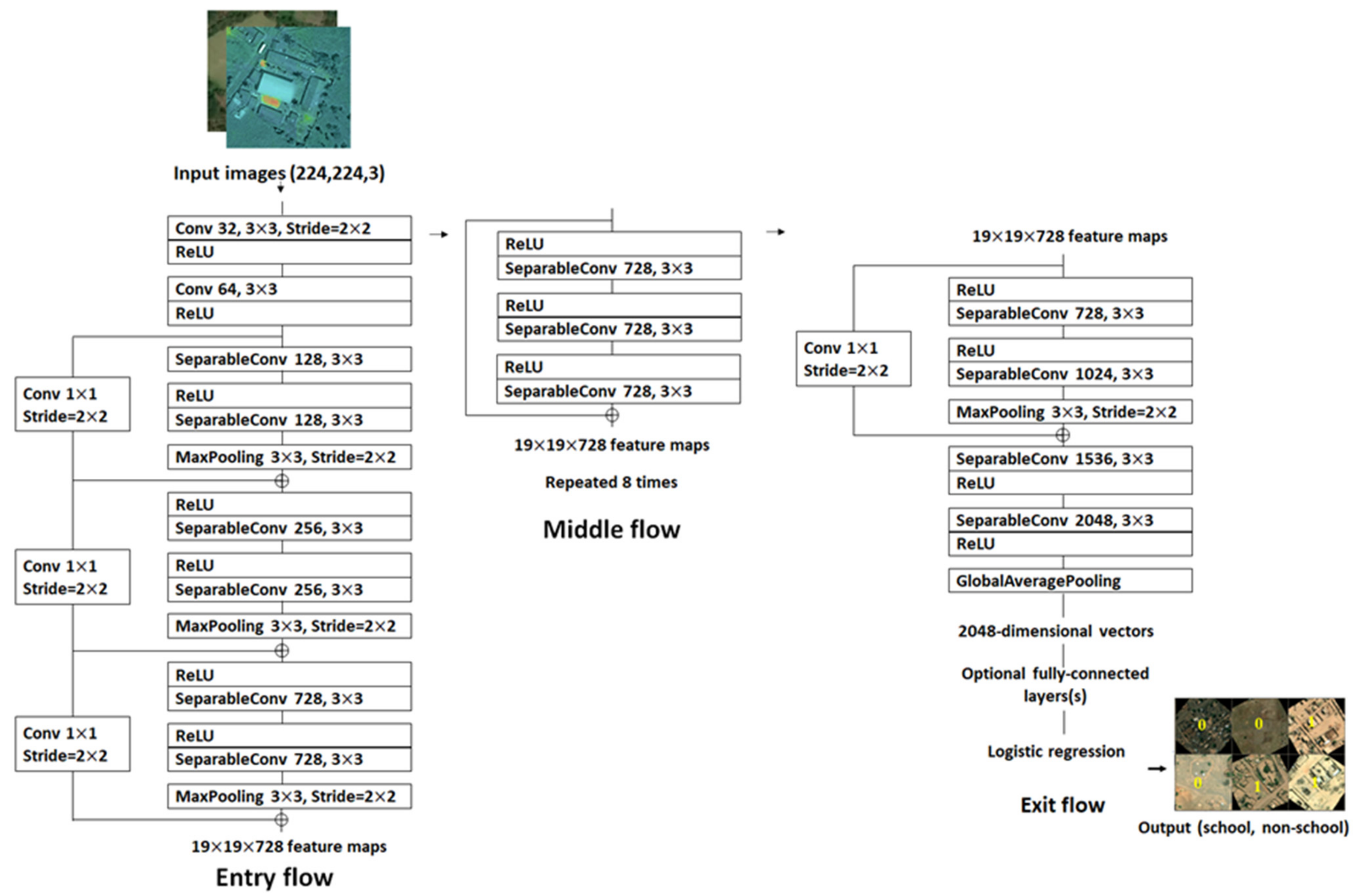
Figure 3.
The Xception network architecture [57].
This workflow is designed to quickly train, transfer-learn, and hyper-tune image classifiers on Google Cloud Kubernetes Engine (GKE) running Kubeflow. The model training and hyper-parameter tuning runs on a Fob YAML file deployment [59].
Figure 3 depicts the Xception network architecture that we adopted from [57]. School and non-school image tiles of 224 × 224 are passed through the network where the first go through the entry flow, through the middle flow which is repeated eight times, and finally through the exit flow for output. An important thing to keep in mind with respect to the Xception network model is that the Convolution and SeparableConvolution layers are followed by batch normalization [7] which were not included in this diagram. Additionally, all SeparableConvolution layers utilizes a depth multiplier of 1 with no depth expansion.
3.1. Datasets
We used a high-resolution satellite image tile of 224 by 224 pixels with zoom level 18 (0.6 m spatial resolution) for each training sample location. The imagery was collected from MAXAR’s imagery archive under NextView license. The imagery collected from Worldview3 sensor was composited with R, G, and B bands using the natural composite method. Numbers of image tiles in various zoom levels used in this study are presented in Section 3.3.
3.2. Training Image Data Preparation
A high-quality training dataset is essential for deep learning approaches to accurately learn through varying object features and generalize precisely. Figure 4 describes the 4-step process of preparing the TFRecords of training image sets for model training.
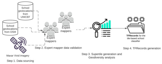
Figure 4.
Steps followed to generate the model training dataset (TFRecords).
Our first step in this regard is to prepare a set of verified school locations, as well as a set of non-school locations in 300 × 300 m image tiles.
- Step 1:
- Data sources
A preliminary list of school locations (coordinates) was acquired from UNICEF ProjectConnect [3] database including data from Rwanda (4233 schools), Sierra Leone (9516), Honduras (17,534), Kazakhstan (7410), and Kenya (20,381). An additional dataset was added (>52,000 schools) from OpenStreetMap from nine different countries as shown in Table 1 below.
- Step 2:
- Training data validation
Five expert mappers reviewed the dataset and compared it to high-resolution satellite imagery. The locations were classified into those where (1) satellite image tiles clearly contain schools as ‘confirmed’, (2) satellite image tiles clearly do not contain a school as ‘not-school’, and (3) it is uncertain whether satellite image tiles contain a school or not as ‘unrecognized’ school, see “Total Point After Validation”, Table 1.
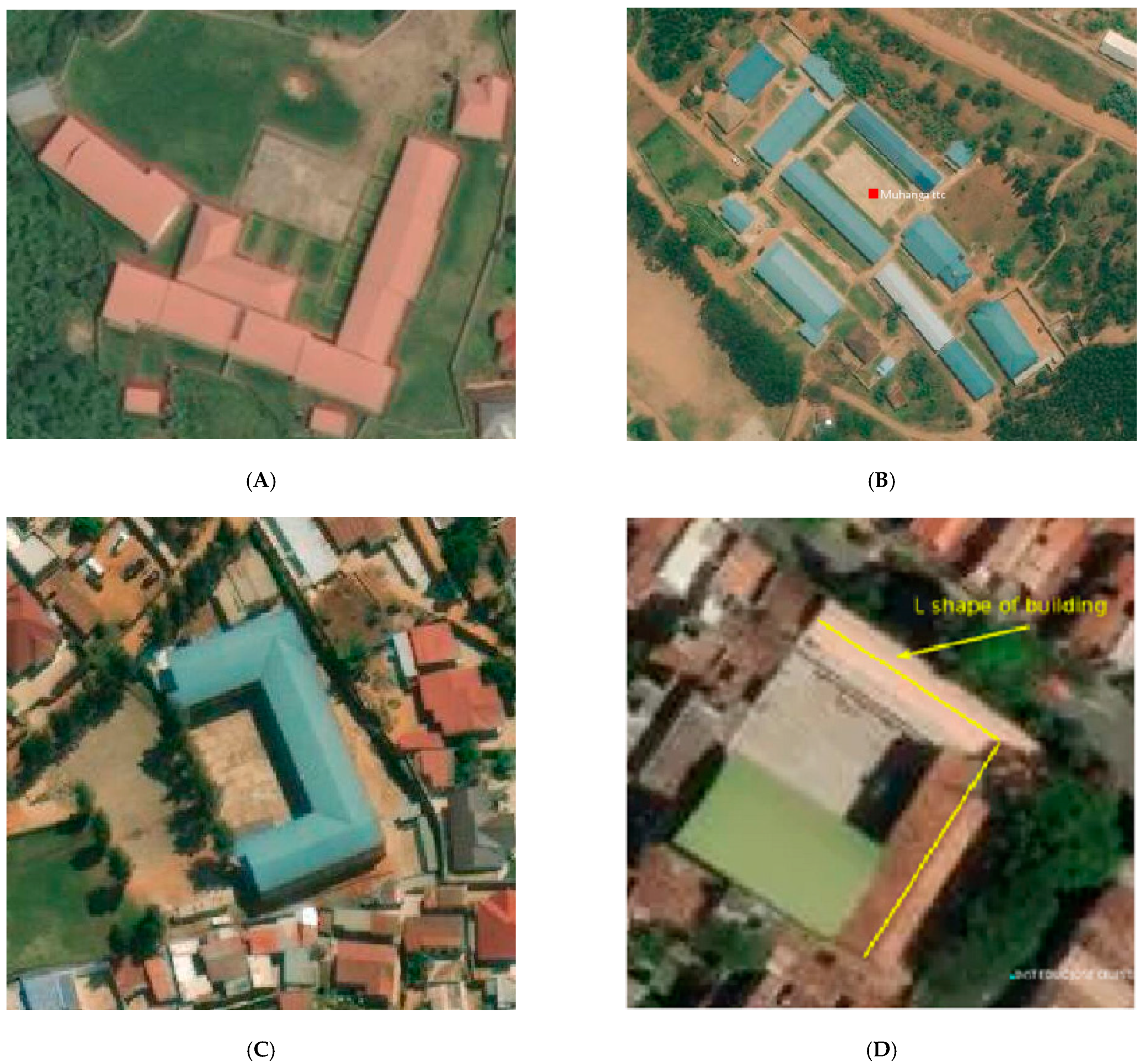
The ‘YES’ school class shows clear school features, e.g., building size, shape, and facilities from the high-resolution satellite imagery. Figure 5 contains some examples of the school features that were used as criteria for schools and that can be used to label the tiles as “confirmed” schools.

Figure 5.
Examples of verified ‘YES’ school image tiles. (A) Building with sport fields, (B) Group of the same type of buildings, (C) Building with U shape, (D) Buildings with L shape and empty field.
The ‘UNRECOGNIZED’ school class refers to school locations that were part of the original country school datasets but that had no clear school features, especially in urban areas with high building density or, in rural areas that cannot be distinguished from residential buildings [2]. Another case of unrecognized schools is school building(s) that cannot be seen on satellite imagery because of cloud/tree cover as shown in Figure 6.
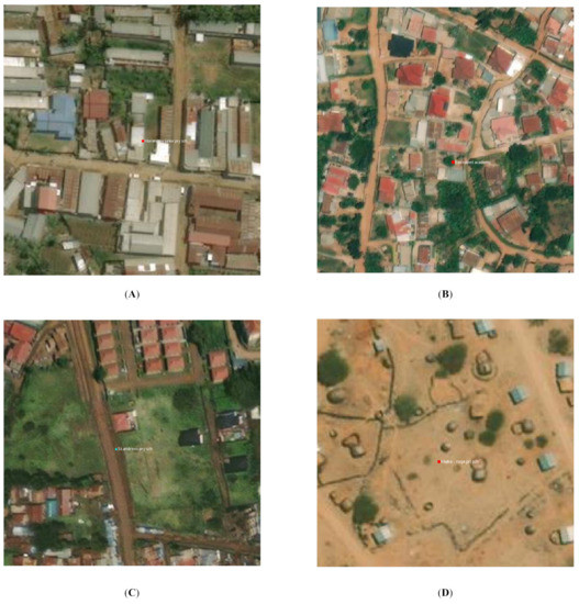
Figure 6.
Examples of verified ‘UNRECOGNIZED’ school image tiles. (A) All buildings look similar, (B) All buildings look similar, (C) School location on the highway, (D) All buildings look as residential (rural).
The ‘No’ schools refer to locations from the original country school datasets where the expert mappers could not find any school-like buildings at the provided school geolocations. As an example, some of the schools were mislocated in the middle of the ocean, desert, dense forest. This can be caused by the school geolocation being recorded incorrectly or because the satellite imagery has been updated in particular areas of the selected countries after schools were built. Examples are shown in Figure 7 below.
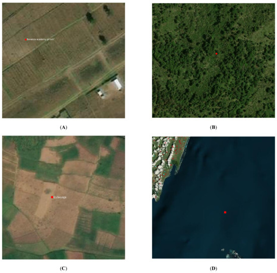
Figure 7.
Examples of verified ‘No’ school image tiles. (A) School location far from residential areas, (B) School location in forest areas, (C) School location in farm fields, (D) School location in the ocean.
- Step 3:
- Training data generation
Training data generated were used for both tile-based image classification and direct school detection. A tile-based school classifier is a binary image classification based on the Xception deep learning backbone from ImageNet [60]. The direct school detection model is an Object Detection model that we based on SSD MobileNet and ResNet101 [61] models.
- Tile-based School Classifier
For the tile-based school classifier model, two categories of datasets were generated, ‘school’ and ‘not-school’, as the training dataset for the deep learning model training. The category ‘school’ tiles were downloaded based on the geolocation of schools that were tagged as “YES” after training data validation (Table 1). Though, the category of “not-school” is more diverse than “school”, because it includes the categories except schools, e.g., forest, desert, critical infrastructure (places of worship, government offices, hospitals, marketplaces, factories), residential buildings, oceans, other water bodies, etc., as shown in Table 2 below. To enrich the data sets for ‘not-school’, we queried all the categories mentioned above from OSM using OSM Map Features [62].
Table 2.
Training datasets for country models that include negative (not-school) and positive (school) categories. Not-school includes buildings from urban and rural, forest, desert, water, and “NO” school tag list in Table 1.
3.3. Supertile Generation
The tile-based school classifier models are trained with the image chips/tiles of OSM slippy map tiles. From our previous experience with an AI school mapping task in Colombia, we found that when a tile is in Zoom 17 [63], the classification model performed the best. The tiles in Zoom 17 are about 300 × 300 m and in the spatial resolution of 1.2 m/pixel. In this study, we maximized the spatial resolution of the satellite image and instead of using Zoom 17, we created a supertile that is made up of 4 zoom 18 tiles as shown in Figure 8. The supertile still represents 300 × 300 m, but by using zoom 18, we have satellite image tiles in the spatial resolution of 0.6 m instead of 1.2 m. Therefore, the school classifier models can learn more image features from high-resolution supertiles.
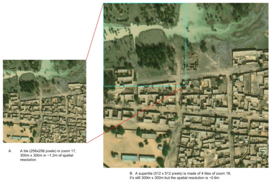
Figure 8.
A sample image supertile.
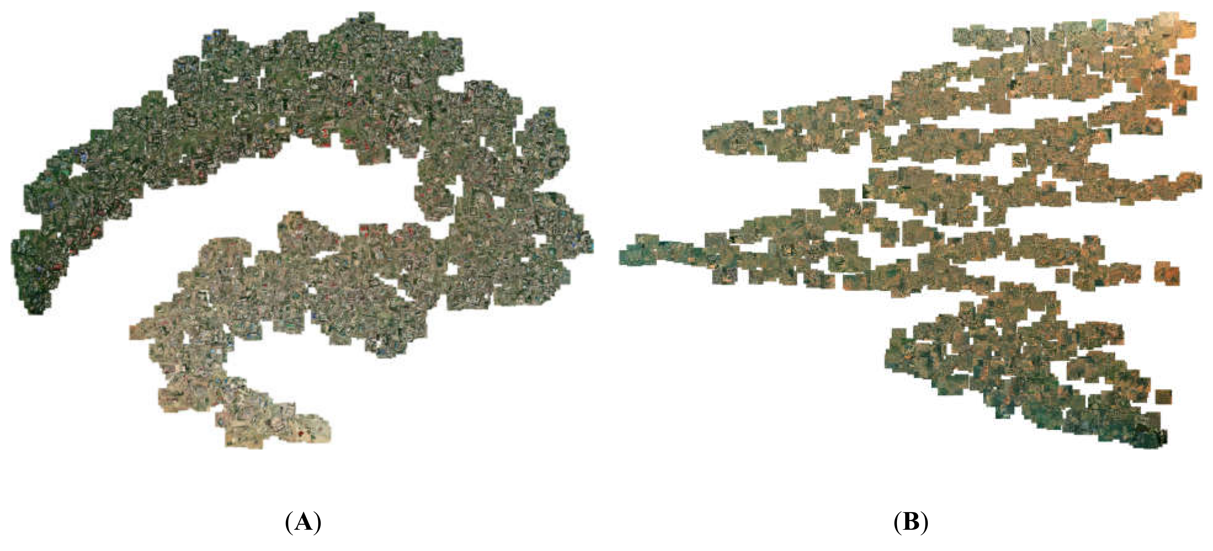
One important factor we put into consideration in generating the training dataset was ‘geodiversity’ of the training image set. This represents the diversity of landscapes that can be captured by the satellite. When it comes to optical images, they are a set of image features that include mountains, vegetation distribution, hurricanes, and smoke patterns. Then we can compare the dataset to the area we want to generalize over based on image similarity metrics such as the t-Distributed Stochastic Neighbor Embedding (t-SNE) [64]. This will help to evaluate whether our training images for the deep learning models are a representative sample of the desired deployment region. In this context, for ‘geodiversity’ of school and not-school for the countries of interest the supertiles can be plotted to showcase the distribution of the data classes from lush-like to desert-like as shown in Figure 9. This is done simply by reducing the image to a single feature vector which is the average RGB value. These vectors are passed to the t-SNE algorithm which is trying to map data to two dimensions (in this case) by computing ‘similarity scores’ to cluster the data, creating a good visual approximation of the original dimension of the data.

Figure 9.
School location diversity analysis through t-SNE shows that the school supertiles stretch from lush-like to desert-like in Kazakhstan and Niger. (A) School location diversity for Kazakhstan, (B) School location diversity for Niger.
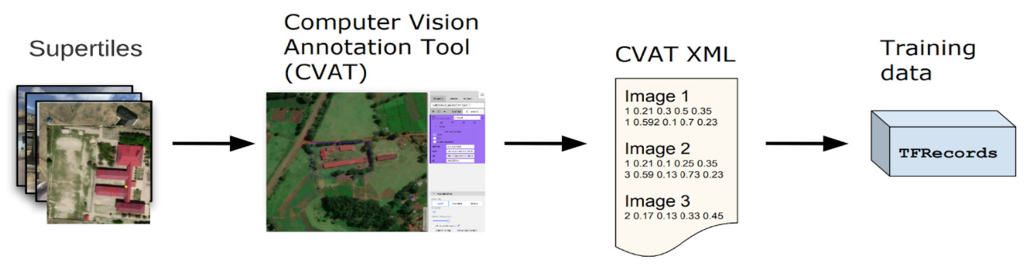
To assess the model performance fairly, our training dataset of two categories, school, and not-school tiles, is then split into a 70:20:10 ratio as train, validation, and test datasets. These three sets of data were generated as TFRecords. TFrecords is a data format that stores a sequence of binary records for Tensorflow [65] to read images and label data efficiently during the model training. The randomly selected 70% of tiles are used to train the model, the remaining 20% are used to validate the model. However, the last 10% of the test dataset which had not been seen by the model acts as the golden standard dataset to evaluate the model performance. For the direct school detection model, the training dataset was created using the Computer Vision Annotation Tool (CVAT) to generate bounding boxes around the school building complex. The resultant XML files were then exported from CVAT and TFRecords were generated for model development as described in Figure 10 below.
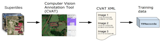
Figure 10.
Training data generation for Kenya direct school detection.
We relied on population data to improve the diversity of training data as well as to identify areas of interest (AOI) to run inference over. This allows us to be efficient in our inference and validation processes. One of the considerations in the training data preparation was to ensure that samples are selected from populated areas. We used a combination of WorldPop [66] and OpenStreetMap. WorldPop is a 100 m spatial resolution contemporary dataset on human population distributions. We translated WorldPop raster pixels as points, and extracted highway, buildings, sports, amenity, leisure, landuse (residential) from OSM and merged the layers and converted them to get zoom 16 populated tiles (see the following Table 3).
Table 3.
Populated tiles in zoom 16 were generated using OSM data and WorldPop.
We end up having 71 million zoom 18 tiles and 18 million supertiles of zoom 17 tiles for all the countries that we needed to run the model inference over.
4. Results
The process of developing the tile-based school classifier model followed a stepwise process by firstly developing and training the global model and assessing the accuracy of generalization based on a dataset from eight countries. The F1 score of the global model is 0.85 over the validation dataset after several hyper-parameter tuning. The need for higher accuracy scores prompted the development of the regional and the country specific models.
The regional model was trained with country datasets that are geo-physically close to each other. For instance, the East African regional model was trained with Kenya and Rwanda datasets, and the West African regional model was trained with Niger, Sudan, Mali, Chad, and Sierra Leone datasets. The regional models outperformed the global and the country-specific models, which indicates that the models were exposed to more diverse school features affirming the fact that the greater variability in the dataset the better the models. The F1 scores of the regional models were greater than 0.91 over the validation dataset.
The trained country models performed well with the validation dataset such that their F1 scores were above 0.9 except for the Niger country model (0.87). The detailed model evaluation metrics, including precision, recall, and F1 scores for each model are tabulated in Table 4 below.
Table 4.
Model evaluation metric report for all the tile-based school classifier models.
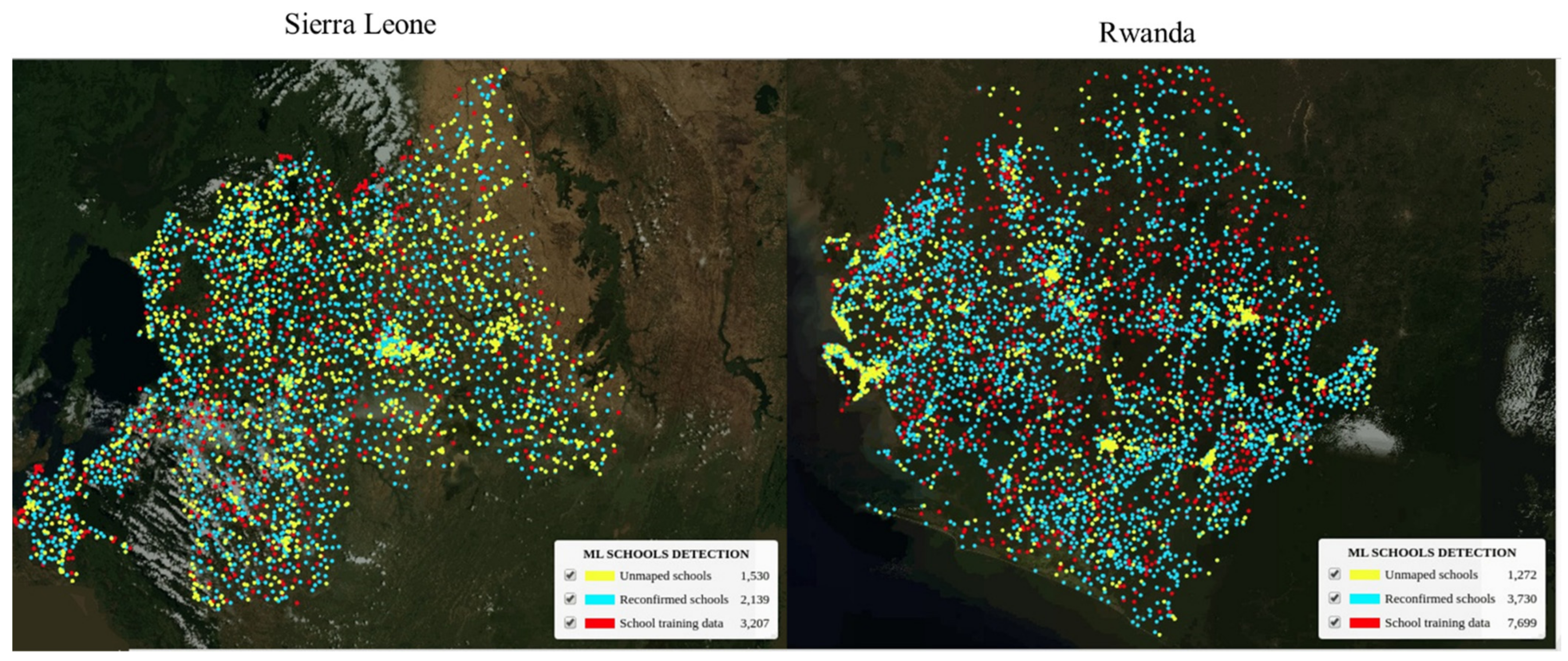
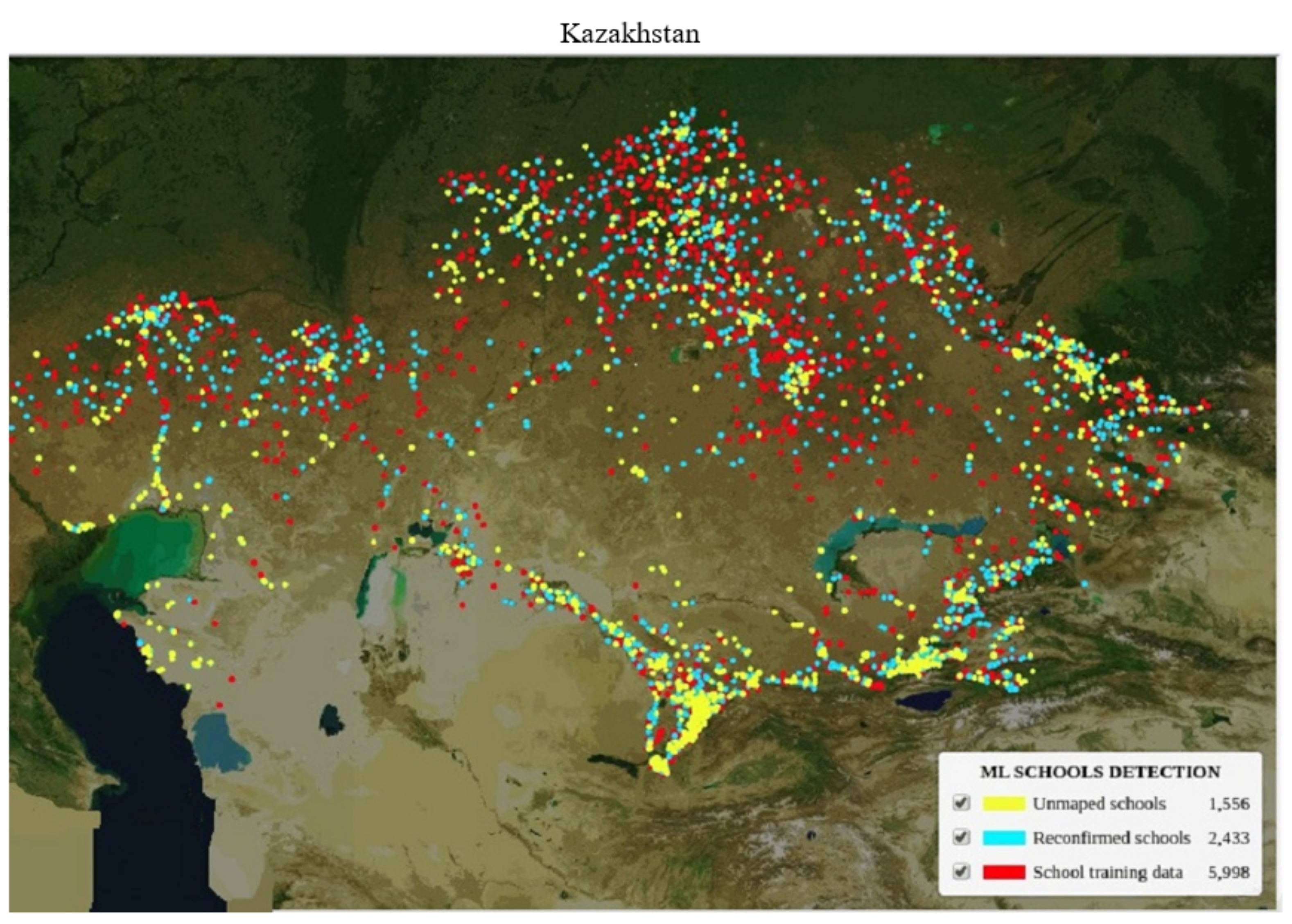
All the country models as well as the regional model performed better than the global model over the validation datasets. Part of the reason is that eight countries alone is not sufficient to train a global model with greater diversity in school structures and features. For a more accurate global model, a dataset from many countries of the world is needed to train the model to increase feature variability and enable the model to generalize well at a global level. However, despite their varying structures, many schools have identifiable overhead signatures that make them possible to detect in high-resolution imagery with deep learning techniques. Approximately 18,000 previously unmapped schools across five African countries (Kenya, Rwanda, Sierra Leone, Ghana, and Niger), were found in satellite imagery with a deep learning classification model. These 18,000 schools were validated by expert mappers and added to the map. We also added and validated nearly 4000 unmapped schools to Kazakhstan and Uzbekistan in Asia, and an additional 1100 schools in Honduras. In addition to finding previously unmapped schools, the models were able to identify already mapped schools up to 80% depending on the country. Figure 11 and Figure 12 show the maps of AI-discovered schools in yellow, existing school locations on OSM reconfirmed by the model shown in blue, and original school locations used to train the models in red.
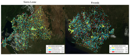
Figure 11.
Map showing AI-discovered schools in Sierra Leone and Rwanda.
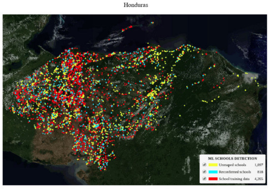
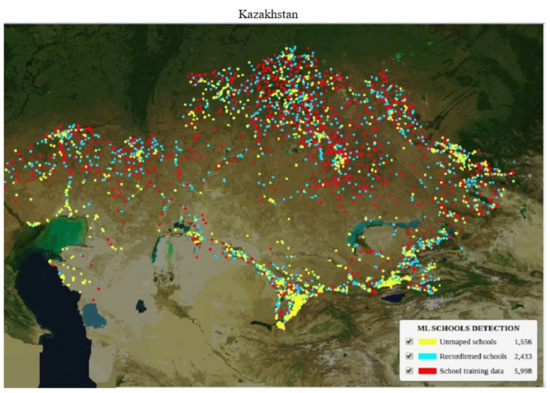
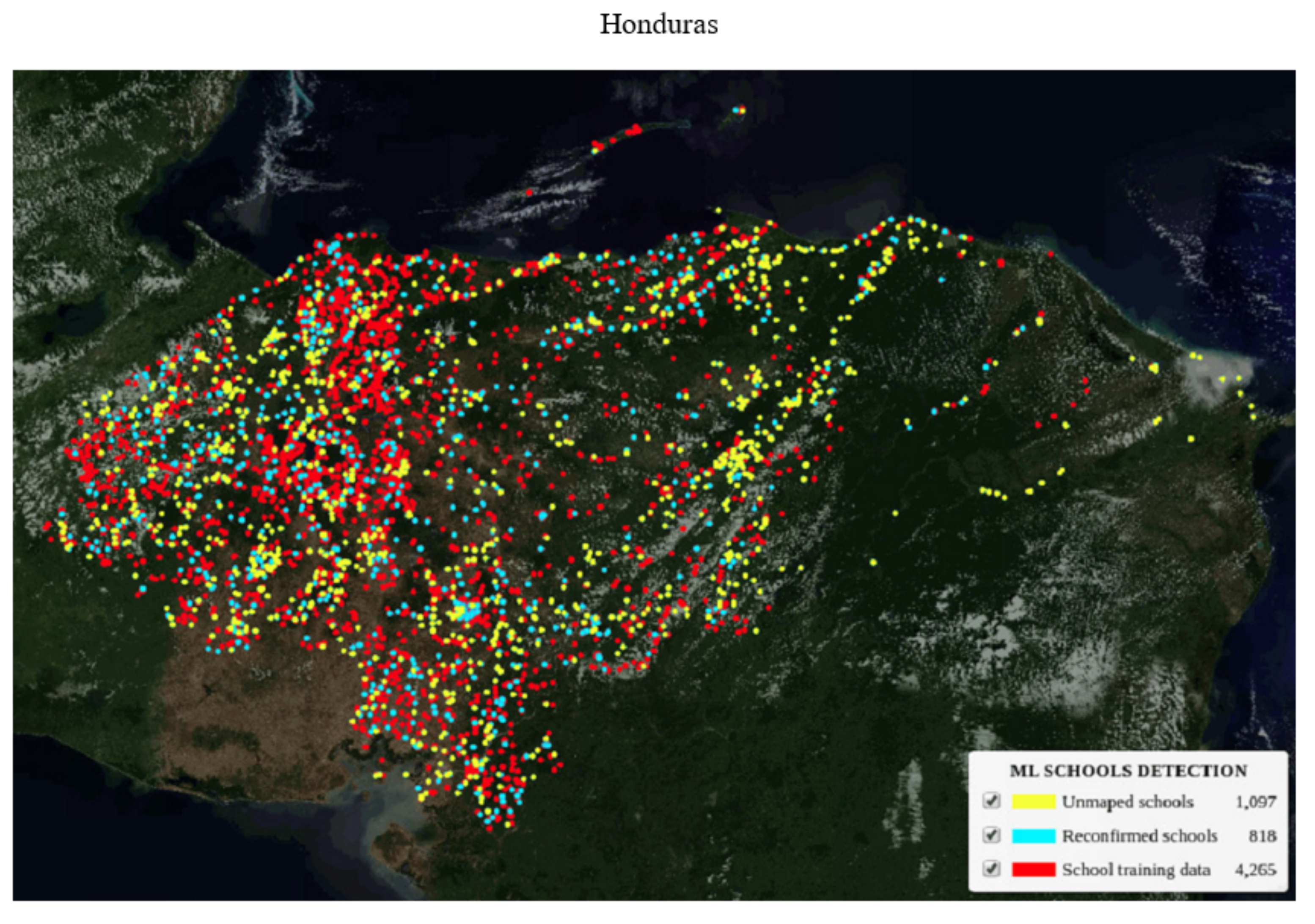
Figure 12.
Map showing AI-discovered schools in Honduras and Kazakhstan.
The detailed findings from tile-based school classifier country models are in the following Table 5.
Table 5.
Model inference summary across different countries.
The column “Known school” presents validated school geolocations that have clear school features. The column “Total detected” shows the total number of detected schools with the given ML threshold scores. The “ML output validation” indicates after the expert mapper’s validation of the ML outputs. The number of confirmed schools “Yes”, unrecognized schools “Un-reg”, and “No” schools. The “True capture” column presents the percentage of known schools that are correctly predicted by ML model and then confirmed by our expert mappers. The higher the percentage means the country ML model performed better.
“Difference” is the number of schools that ML models did not find but are in “Known school”. “Reconfirmed” is the number of schools detected by ML models, validated by the expert mappers, and are also in the “Known school”. The Unmapped schools are the schools that currently are NOT on the map or in “Known school” but detected by ML models and validated by the expert mappers.
Differences in Model Performances
Kenya is the only country that has over 20,000 known schools that have been validated by expert mappers. Only 6000 schools in Kenya were randomly selected to train the Kenya country model.
It means that there are more than 14,000 known schools left over as “test data” that were never exposed to the model. Therefore, Kenya is the perfect country to answer questions including:
- ○
- How do regional and country models perform differently?
- ○
- Is it necessarily true to build country-specific models or can we rely on only the regional model that is generalized well across countries?
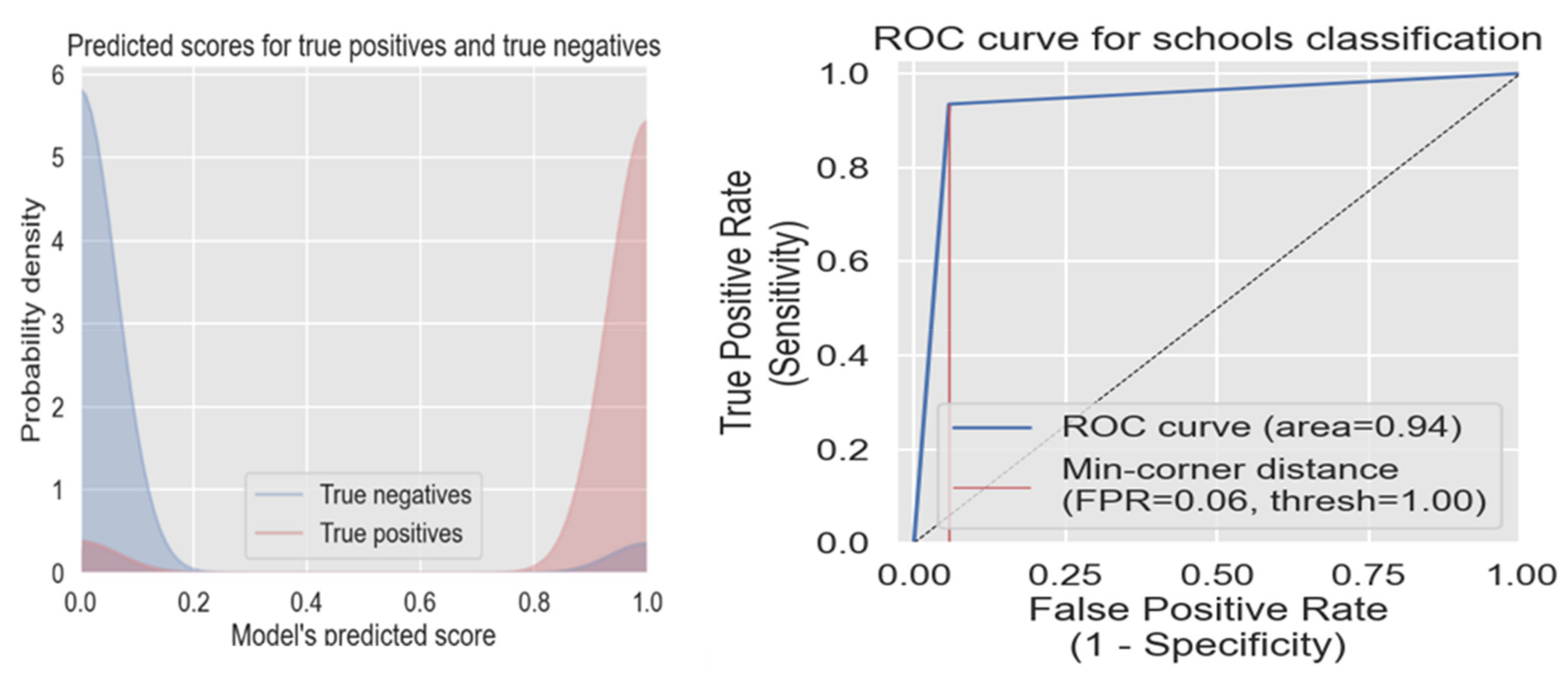
Figure 13 shows the true positive and negative of the model performance in Kenya (on the left); the model was able to separate the two categories well. The ROC curve (on the right) for the Kenya country model tells us that when we use the DNN threshold of 1.0, there will only be a 6% false-positive rate.
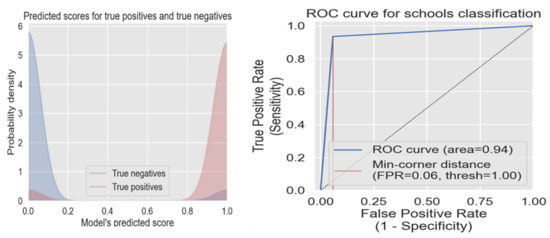
Figure 13.
True positive, true negative scores, and ROC curve of the Kenyan model.
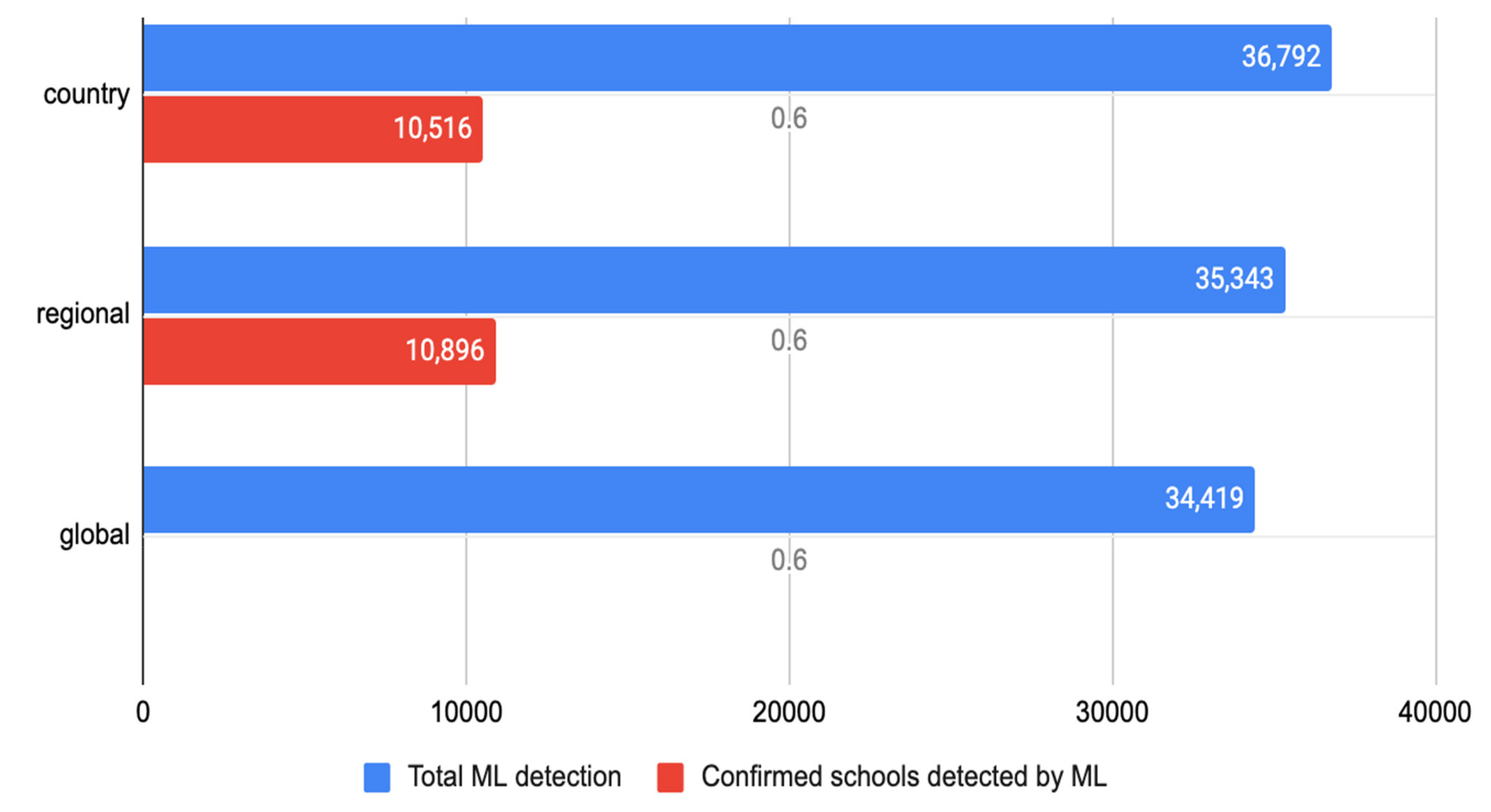
By plotting the results from the Kenya model, inferences with the Kenya country, East African regional and global models, we found that the regional model outperformed the country model in that it produced fewer ML-detected schools (Figure 14-blue bar), which means fewer false positives. It was able to detect more schools (the red bar) that fell under unknown schools.
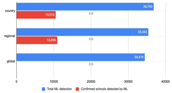
Figure 14.
Model performance in Kenya.
- -
- Both country and regional models performed very well even though the models were only exposed to a quarter of the available known schools in Kenya. Figure 13 also showed that the global model had more false negatives with less true and false positives when compared with the country and regional models, respectively. There is only the blue bar for the global model in the figure because the model result validation has not been done yet due to the lack of man-hours, but we have plans to do that as soon we have the capacity.
- -
- In the future, model transfer-learning or fine-tuning will be used to train a regional model instead of developing country-specific models.
5. Discussion
In this section, we discuss some of the challenges that were faced in terms of model scalability, pros and cons of the AI models, the roadmap for the future work that may involve human-in-the-loop and active learning methods.
5.1. Model Scalability
To develop global scale school classifier, the scalability context is non-trivial.
Some of the scalability challenges in developing models that can generalize from country to country, urban to rural from diverse school features and millions of image tiles were handled from the context of hyper-parameter optimization by exploring variations in model architecture, loss functions, regularization, pre-training and post-processing to increase the model performance.
Additionally, data tooling, best practices in model training, and inference speed helped to increase the scalability of the models across the globe. Massive data validation exercises over geo-diverse landscapes and varying school structures from rural to urban, from culture to culture, and nation to nation were important factors that positively influenced the model’s generalizability and scalability. The models were trained with diverse selected school features to create a generalized model that can search for school-like building complexes from millions of satellite image tiles across the regions. We also made some important contributions around the technical challenges of scaling school classifiers in very high-resolution imagery to the country- and continent-wide applications. We were able to solve model technical scalability issues by mindfully designing the internal data validation, model training on Google Kubernetes Cluster Engines (GKE) with Kubeflow, and model inference with our open-sourced tools. We have also started working on a roadmap for addressing remaining technical challenges around model generalizability especially with the global model which could not be generalized as well as the regional and country models. This roadmap includes increasing the global sample training data to encompass diverse school structures from each country of the world, more hyperparameter optimization, human-in-the-loop, and active learning methods.
5.2. Comparative Performance of Our Xception Network Model
We further carried out a performance comparative analysis of our Xception network model with other two state-of-the-art deep learning networks, the MobileNet and ResNet 152 which have been ranked on par with the Xception Network [60]. This exercise became essential to scientifically justify our choice of the Xception network model and to ascertain the claim from ImageNet [60] literature that Xception was better than the rest in terms of performance accuracy. This test was carried out on the Sudan school training dataset of over 16,400 image tiles (6400 schools and 10,000 non-schools) of 224 × 224 size, and ran on the same AzureML GPU configuration over 25 training epochs.
Though all three networks produced great accuracy as well as their F1 score, precision, and recall, our Xception network performed slightly better as shown in Table 6. This 0.003 improvement in accuracy means a lot to us in terms of the number of false positives and false negatives we were able to reduce as compared to using MobileNet and RestNet networks. The Xception network reduced the number of false positives from the MobileNet model by 15%, that of ResNet by 11%, and the false negative was reduced by 19% and 14% for MobileNet and ResNet networks, respectively. For humanitarian purposes where higher accuracy is paramount [6] and efforts are made to minimize false positives and negatives, this is significant.
Table 6.
Xception comparative performance against MobileNet-v2 and ResNet 152.
5.3. AI-Assisted School Mapping Pros and Cons
AI and ML models are particularly good at recognizing the image features they have been exposed to. Schools are like other building infrastructure, and they have their primary purpose. They provide functions such as public gatherings, public recreation, shelter, and even polling stations. Therefore, schools may have unique features that other buildings do not have. From overhead imagery they can show as U, O, I, H shapes, as they have basketball courts, playgrounds, swimming pools or a cluster of buildings with same roof color. The building size is bigger compared to surrounding residential buildings. AI models can be trained to recognize school buildings very well. At the same time, we can utilize cloud computing and modern deep learning techniques to speed up model training and inference that can scan and search for schools rapidly. However, distinguished school features that have been feature engineered to train the models could introduce human bias to the model. In the end, the model may be able to recognize schools that are in distinguished building complexes, have similar building rooftops, swimming pools, or basketball courts, but are really bad at recognizing schools that have smaller building sizes and in poorer neighborhoods or even densely populated urban areas.
A limitation of our approach, therefore, is that it relies on human validators for both the training data creation and school validation. As a result, we acknowledge that we introduced a bias for schools that follow common patterns and are recognizable from space. In the end, the model may be able to recognize schools that are in distinguished building complexes, have similar building rooftops, swimming pools, or basketball courts, but may perform poorly at recognizing schools that have smaller building sizes, are in densely populated urban areas, or are housed in “non-traditional” structures. It is reasonable to assume that this bias might disproportionately miss schools that serve poorer neighborhoods or already underrepresented communities. This bias would not exist in alternative (and likely more costly) approaches such as field surveys and supporting community mapping.
Using a human-in-the-loop process is critical, especially leveraging people with local knowledge about local school features. Such knowledge is harder to transfer to expert mappers who may grow up in a different culture and architectural context of schools. We engaged in active research and development of human-in-the-loop active learning methods that allow non-expert human mappers and AI to work more efficiently together and improve the model’s prediction power. By creating greater accessibility to providing human input into these models, we hope to increase the diversity of human knowledge contributing to these models and reduce sources of bias. An active learning platform that allows human–AI to work together and improve the model prediction power is the next phase of this study, considering that we have developed all the necessary tooling and technology under this phase of the work that will help us to achieve the next goal.
5.4. Conclusions
This study aimed at developing rapid and scalable AI models that can deliver automated and swift mapping of schools using high resolution satellite imagery at country-wide, regional, and even global scales. The study was designed to apply scalable deep learning techniques over high-resolution satellite imagery to map schools globally with the aim to help accelerate the Giga (UNCEF and ITU) initiative and mission to connect every school to the internet and reduce the global digital divide across schools.
In spite of the varying features of school locations across countries and regions, this study proved that there are still yet identifiable overhead signatures common to school locations that made it possible to detect schools from high-resolution satellite imagery with modern deep learning techniques.
Furthermore, one of the contributions of this study is also to test the generalizability of different DNN models in identifying the presence of these school features from satellite image snapshots. For example, we were interested in finding out if the digital signature of school locations in Colombia are close enough to those of neighboring countries such that a model trained on Colombia data can be used to identify school locations in neighboring countries. We tested this by using the model developed in Colombia to detect schools in 11 Eastern Caribbean nations including Anguilla, Antigua, Barbuda, British Virgin Islands, Dominica, Grenada, The Grenadines, Montserrat, St Kitts and Nevis, St Lucia, and St Vincent. The model did not only find already mapped schools in these Caribbean nations but was also able to identify previously unmapped schools with more than 80% precision and recall.
The DNN models we developed in this study which are based on the Xception architecture produced satisfactory performance for the target use, especially at regional and country level inferences. As future work, we plan to improve the global model using an object-based (vectorized training dataset instead of image tile) approach.
Author Contributions
Z.Y., D.-H.K., I.M., N.Z., C.F. designed the research, Z.Y., D.-H.K., I.M. implemented the design, I.M., D.-H.K., S.A. wrote the manuscript, and all the authors edited the manuscript. All authors have read and agreed to the published version of the manuscript.
Funding
This research received no external funding.
Data Availability Statement
Data used for this research cannot be made open source.
Acknowledgments
We would like to acknowledge the Giga (UNICEF and ITU) initiative for providing the internal funding and platform that made this research work possible. Maxar’s high-resolution satellite imagery used for this work were provided by the United States Government under NextView end user license.
Conflicts of Interest
The authors declare no conflict of interest.
References
- UN General Assembly; Transforming Our Development; Sustainable Development; Sustainable Development Goals; World Bank; World Economic Forum. Sustainable Development Goal 4 Education Brief: SDG4; UNHCR: Geneva, Switzerland, 2015. [Google Scholar]
- Zhuangfang, S.A.; Yi, N.; Zurutuza, N.; Kim, D.-H.; Mendoza, R.L.; Morrissey, M.; Daniels, C.; Ingalls, N.; Farias, J.; Tenorio, K.; et al. Building on Our Success Mapping 23,100 Unmapped Schools in Eight Countries. Available online: https://developmentseed.org/blog/2021-03-18-ai-enabling-school-mapping (accessed on 15 December 2021).
- Connecting Every School in the World to the Internet. Available online: https://projectconnect.unicef.org/map (accessed on 12 November 2021).
- Chen, B.; Tu, Y.; Song, Y.; Theobald, D.M.; Zhang, T.; Ren, Z.; Li, X.; Yang, J.; Wang, J.; Wang, X.; et al. Mapping essential urban land use categories with open big data: Results for five metropolitan areas in the United States of America. ISPRS J. Photogramm. Remote Sens. 2021, 178, 203–218. [Google Scholar] [CrossRef]
- Tu, Y.; Chen, B.; Lang, W.; Chen, T.; Li, M.; Zhang, T.; Xu, B. Uncovering the Nature of Urban Land Use Composition Using Multi-Source Open Big Data with Ensemble Learning. Remote Sens. 2021, 13, 4241. [Google Scholar] [CrossRef]
- Kim, D.-H.; López, G.; Kiedanski, D.; Maduako, I.; Ríos, B.; Descoins, A.; Zurutuza, N.; Arora, S.; Fabian, C. Bias in Deep Neural Networks in Land Use Characterization for International Development. Remote Sens. 2021, 13, 2908. [Google Scholar] [CrossRef]
- Chollet, F. Xception: Deep Learning with Depthwise Separable Convolutions. In Proceedings of the 2017 IEEE Conference on Computer Vision and Pattern Recognition (CVPR), Honolulu, HI, USA, 21–26 July 2017; pp. 1800–1807. [Google Scholar]
- Howard, A.G.; Zhu, M.; Chen, B.; Kalenichenko, D.; Wang, W.; Weyand, T.; Andreetto, M.; Adam, H. MobileNets: Efficient Convolutional Neural Networks for Mobile Vision Applications. arXiv 2012, arXiv:1704.04861. [Google Scholar]
- Hoeser, T.; Bachofer, F.; Kuenzer, C. Object Detection and Image Segmentation with Deep Learning on Earth Observation Data: A Review—Part II: Applications. Remote Sens. 2020, 12, 3053. [Google Scholar] [CrossRef]
- Goupilleau, A.; Ceillier, T.; Corbineau, M.-C. Active learning for object detection in high-resolution satellite images. arXiv 2021, arXiv:2101.02480. [Google Scholar]
- Abdollahi, A.; Pradhan, B.; Shukla, N.; Chakraborty, S.; Alamri, A. Deep Learning Approaches Applied to Remote Sensing Datasets for Road Extraction: A State-Of-The-Art Review. Remote Sens. 2020, 12, 1444. [Google Scholar] [CrossRef]
- Voulodimos, A.; Doulamis, N.; Doulamis, A.; Protopapadakis, E. Deep Learning for Computer Vision: A Brief Review. Comput. Intell. Neurosci. 2018, 2018, 7068349. [Google Scholar] [CrossRef]
- Ekim, B.; Sertel, E.; Kabadayi, M.E. Automatic Road Extraction from Historical Maps Using Deep Learning Techniques: A Regional Case Study of Turkey in a German World War II Map. ISPRS Int. J. Geo Inf. 2021, 10, 492. [Google Scholar] [CrossRef]
- Lima, B.; Ferreira, L.; Moura, J.M. Helping to detect legal swimming pools with deep learning and data visualization. Procedia Comput. Sci. 2021, 181, 1058–1065. [Google Scholar] [CrossRef]
- Abderrahim, N.Y.Q.; Abderrahim, S.; Rida, A. Road Segmentation using U-Net architecture. In Proceedings of the 2020 IEEE International conference of Moroccan Geomatics (Morgeo), Casablanca, Morocco, 11–13 May 2020; pp. 1–4. [Google Scholar]
- Reddy, M.J.B.; Mohanta, D.K. Condition monitoring of 11 kV distribution system insulators incorporating complex imagery using combined DOST-SVM approach. IEEE Trans. Dielectr. Electr. Insul. 2013, 20, 664–674. [Google Scholar] [CrossRef]
- Mahony, N.O.; Campbell, S.; Carvalho, A.; Harapanahalli, S.; Hernandez, G.V.; Krpalkova, L.; Riordan, D.; Walsh, J. Deep Learning vs. Traditional Computer Vision BT. In Advances in Computer Vision Proceedings of the 2019 Computer Vision Conference (CVC), Las Vegas, NV, USA, 25–26 April 2019; Springer Nature Switzerland AG: Cham, Switzerland, 2019; pp. 128–144. [Google Scholar]
- Alzubaidi, L.; Zhang, J.; Humaidi, A.J.; Al-Dujaili, A.; Duan, Y.; Al-Shamma, O.; Santamaría, J.; Fadhel, M.A.; Al-Amidie, M.; Farhan, L. Review of deep learning: Concepts, CNN architectures, challenges, applications, future directions. J. Big Data 2021, 8, 53. [Google Scholar] [CrossRef]
- Garcia-Garcia, A.; Orts-Escolano, S.; Oprea, S.; Villena-Martinez, V.; Rodriguez, J.G. A Review on Deep Learning Techniques Applied to Semantic Segmentation. arXiv 2017, arXiv:1704.06857. [Google Scholar]
- Grinias, I.; Panagiotakis, C.; Tziritas, G. MRF-based segmentation and unsupervised classification for building and road detection in peri-urban areas of high-resolution satellite images. ISPRS J. Photogramm. Remote Sens. 2016, 122, 145–166. [Google Scholar] [CrossRef]
- Maduako, I.; Igwe, C.; Abah, J.; Onwuasoanya, O.; Chukwu, G.; Ezeji, F.; Okeke, F. Deep Learning for Component Fault Detection in Electricity Lines Transmission. J. Big Data 2021. [Google Scholar] [CrossRef]
- Stewart, C.; Lazzarini, M.; Luna, A.; Albani, S. Deep Learning with Open Data for Desert Road Mapping. Remote Sens. 2020, 12, 2274. [Google Scholar] [CrossRef]
- Henry, C.; Azimi, S.M.; Merkle, N. Road Segmentation in SAR Satellite Images with Deep Fully Convolutional Neural Networks. IEEE Geosci. Remote Sens. Lett. 2018, 15, 1867–1871. [Google Scholar] [CrossRef] [Green Version]
- Yuan, M.; Liu, Z.; Wang, F. Using the wide-range attention U-Net for road segmentation. Remote Sens. Lett. 2019, 10, 506–515. [Google Scholar] [CrossRef]
- Yang, X.; Li, X.; Ye, Y.; Lau, R.Y.K.; Zhang, X.; Huang, X. Road Detection and Centerline Extraction Via Deep Recurrent Convolutional Neural Network U-Net. IEEE Trans. Geosci. Remote Sens. 2019, 57, 7209–7220. [Google Scholar] [CrossRef]
- Şen, N.; Olgun, O.; Ayhan, Ö. Road and railway detection in SAR images using deep learning. In Image and Signal Processing for Remote Sensing XXV; SPIE: Bellingham, WA, USA, 2019; Volume 11155, pp. 125–129. [Google Scholar]
- Cheng, G.; Wang, Y.; Xu, S.; Wang, H.; Xiang, S.; Pan, C. Automatic Road Detection and Centerline Extraction via Cascaded End-to-End Convolutional Neural Network. IEEE Trans. Geosci. Remote Sens. 2017, 55, 3322–3337. [Google Scholar] [CrossRef]
- Zhang, L.; Wang, P.; Shen, C.; Liu, L.; Wei, W.; Zhang, Y.; van den Hengel, A. Adaptive Importance Learning for Improving Lightweight Image Super-Resolution Network. Int. J. Comput. Vis. 2020, 128, 479–499. [Google Scholar] [CrossRef] [Green Version]
- Wu, Z.; Wang, X.; Gonzalez, J.E.; Goldstein, T.; Davis, L.S. ACE: Adapting to Changing Environments for Semantic Segmentation. arXiv 2019, arXiv:1904.06268. [Google Scholar]
- Ronneberger, O.; Fischer, P.; Brox, T. U-Net: Convolutional Networks for Biomedical Image Segmentation. arXiv 2015, arXiv:1505.04597. [Google Scholar]
- Remi, D.; Romain, G. Cnns fusion for building detection in aerial images for the building detection challenge. In Proceedings of the IEEE Conference on Computer Vision and Pattern Recognition Workshops, Salt Lake City, UT, USA, 18–23 June 2018; pp. 242–246. [Google Scholar]
- Ivanovsky, L.; Khryashchev, V.; Pavlov, V.; Ostrovskaya, A. Building detection on aerial images using U-NET neural networks. In Proceedings of the Conference of Open Innovation Association FRUCT, Helsinki, Finland, 5–8 November 2019; Institute of Electrical and Electronics Engineers (IEEE): New York, NY, USA, 2019; Volume 2019, pp. 116–122. [Google Scholar]
- Chhor, G.; Aramburu, C.B. Satellite Image Segmentation for Building Detection Using U-Net, 1–6. 2017. Available online: http://cs229.stanford.edu/proj2017/final-reports/5243715.pdf (accessed on 20 January 2022).
- Zhang, Q.; Kong, Q.; Zhang, C.; You, S.; Wei, H.; Sun, R.; Li, L. A new road extraction method using Sentinel-1 SAR images based on the deep fully convolutional neural network. Eur. J. Remote Sens. 2019, 52, 572–582. [Google Scholar] [CrossRef] [Green Version]
- Zhao, Z.; Xu, G.; Qi, Y.; Liu, N.; Zhang, T. Multi-patch deep features for power line insulator status classification from aerial images. In Proceedings of the 2016 International Joint Conference on Neural Networks, {IJCNN} 2016, Vancouver, BC, Canada, 24–29 July 2016; pp. 3187–3194. [Google Scholar]
- Lee, H.; Park, M.; Kim, J. Plankton classification on imbalanced large-scale database via convolutional neural networks with transfer learning. In Proceedings of the 2016 IEEE International Conference on Image Processing (ICIP), Phoenix, AZ, USA, 25–28 September 2016; pp. 3713–3717. [Google Scholar]
- Pouyanfar, S.; Tao, Y.; Mohan, A.; Tian, H.; Kaseb, A.S.; Gauen, K.; Dailey, R.; Aghajanzadeh, S.; Lu, Y.; Chen, S.; et al. Dynamic Sampling in Convolutional Neural Networks for Imbalanced Data Classification. In Proceedings of the 2018 IEEE Conference on Multimedia Information Processing and Retrieval (MIPR), Miami, FL, USA, 10–12 April 2018; pp. 112–117. [Google Scholar]
- Huang, C.; Li, Y.; Loy, C.C.; Tang, X. Learning Deep Representation for Imbalanced Classification. In Proceedings of the 2016 IEEE Conference on Computer Vision and Pattern Recognition (CVPR), Las Vegas, NV, USA, 27–30 June 2016; pp. 5375–5384. [Google Scholar]
- Van Rest, O.; Hong, S.; Kim, J.; Meng, X.; Chafi, H. PGQL: A property graph query language. In ACM International Conference Proceeding Series; Association for Computing Machinery: New York, NY, USA, 2016; Volume 24. [Google Scholar] [CrossRef]
- Buda, M.; Maki, A.; Mazurowski, M.A. A systematic study of the class imbalance problem in convolutional neural networks. Neural Netw. 2018, 106, 249–259. [Google Scholar] [CrossRef] [Green Version]
- Pereira, R.M.; Costa, Y.M.G.; Silla, C.N., Jr. Toward hierarchical classification of imbalanced data using random resampling algorithms. Inf. Sci. 2021, 578, 344–363. [Google Scholar] [CrossRef]
- Bai, R.; Cao, H.; Yu, Y.; Wang, F.; Dang, W.; Chu, Z. Insulator Fault Recognition Based on Spatial Pyramid Pooling Networks with Transfer Learning (Match 2018). In Proceedings of the 2018 3rd International Conference on Advanced Robotics and Mechatronics (ICARM), Singapore, 18–20 July 2018; pp. 824–828. [Google Scholar]
- Ma, L.; Xu, C.; Zuo, G.; Bo, B.; Tao, F. Detection Method of Insulator Based on Faster R-CNN. In Proceedings of the 2017 IEEE 7th Annual International Conference on CYBER Technology in Automation, Control, and Intelligent Systems, CYBER 2017, Kaiulani, HA, USA, 31 July–4 August 2017; pp. 1410–1414. [Google Scholar]
- Gu, J.; Wang, Z.; Kuen, J.; Ma, L.; Shahroudy, A.; Shuai, B.; Liu, T.; Wang, X.; Wang, G.; Cai, J.; et al. Recent advances in convolutional neural networks. Pattern Recognit. 2018, 77, 354–377. [Google Scholar] [CrossRef] [Green Version]
- Jiang, H.; Qiu, X.; Chen, J.; Liu, X.; Miao, X.; Zhuang, S. Insulator Fault Detection in Aerial Images Based on Ensemble Learning with Multi-Level Perception. IEEE Access 2019, 7, 61797–61810. [Google Scholar] [CrossRef]
- Gonzalez, T.F. Handbook of Approximation Algorithms and Metaheuristics; CRC Press: Boca Raton, FL, USA, 2017; pp. 1–1432. [Google Scholar]
- Simonyan, K.; Zisserman, A. Very deep convolutional networks for large-scale image recognition. In Proceedings of the 3rd International Conference on Learning Representations, ICLR 2015, San Diego, CA, USA, 7–9 May 2015. [Google Scholar]
- He, K.; Zhang, X.; Ren, S.; Sun, J. Deep residual learning for image recognition. Proc. IEEE Comput. Soc. Conf. Comput. Vis. Pattern Recognit. 2016, 2016, 770–778. [Google Scholar]
- Rosebrock, A. Deep Learning for Computer Vision with Python (ImageNet). In Deep Learning for Computer Vision with Python 3; PyImageSearch: Nice, France, 2017. [Google Scholar]
- Ren, S.; He, K.; Girshick, R.; Sun, J. Faster R-CNN2015. Biol. Conserv. 2015, 158, 196–204. [Google Scholar]
- Dai, J.; Li, Y.; He, K.; Sun, J. R-FCN: Object Detection via Region-based Fully Convolutional Networks. arXiv 2016, arXiv:1605.06409. [Google Scholar]
- Liu, Y.; Pei, S.; Fu, W.; Zhang, K.; Ji, X.; Yin, Z. The discrimination method as applied to a deteriorated porcelain insulator used in transmission lines on the basis of a convolution neural network. IEEE Trans. Dielectr. Electr. Insul. 2017, 24, 3559–3566. [Google Scholar] [CrossRef]
- Chollet, F. Deep Learning with Python; Manning Publications: Shelter Island, NY, USA, 2017. [Google Scholar]
- Redmon, J.; Divvala, S.; Girshick, R.; Farhadi, A. You only look once: Unified, real-time object detection. Proc. IEEE Comput. Soc. Conf. Comput. Vis. Pattern Recognit. 2016, 2016, 779–788. [Google Scholar]
- Liu, W.; Anguelov, D.; Erhan, D.; Szegedy, C.; Reed, S.; Fu, C.; Berg, A.C. SSD: Single Shot MultiBox Detector. Lect. Notes Comput. Sci. 2018, 9905, 21–37. [Google Scholar]
- Simonyan, K.; Zisserman, A. Very Deep Convolutional Networks for Large-Scale Image Recognition. arXiv 2015, arXiv:1409.1556. [Google Scholar]
- Chollet, F. Xception: Deep Learning with Depthwise Separable Convolutions; IEEE: New York, NY, USA, 2017. [Google Scholar]
- Chollet, F. Keras [Internet]. GitHub. 2015. Available online: https://github.com/fchollet/keras (accessed on 15 December 2021).
- Skaffold.yaml. Available online: https://skaffold.dev/docs/references/yaml/ (accessed on 15 December 2021).
- Deng, J.; Dong, W.; Socher, R.; Li, L.-J.; Li, K.; Fei-Fei, L. Imagenet: A large-scale hierarchical image database. In Proceedings of the 2009 IEEE Conference on Computer Vision and Pattern Recognition, Miami, FL, USA, 20–25 June 2009; pp. 248–255. [Google Scholar]
- He, K.; Zhang, X.; Ren, S.; Sun, J. Deep Residual Learning for Image Recognition. arXiv 2015, arXiv:1512.03385. [Google Scholar]
- OSM, Map Features, OpenStreetMap Wiki. Available online: https://wiki.openstreetmap.org/wiki/Map_features (accessed on 20 October 2021).
- OSM, Zoom levels, OpenStreetMap Wiki. Available online: https://wiki.openstreetmap.org/wiki/Zoom_levels (accessed on 24 October 2021).
- Van der Maaten, L.; Hinton, G. Visualizing Data using t-SNE. J. Mach. Learn. Res. 2008, 9, 2579–2605. [Google Scholar]
- Shanmugamani, R.; Rahman, A.G.A.; Moore, S.M.; Koganti, N. Deep Learning for Computer Vision: Expert Techniques to Train Advanced Neural Networks Using Tensorflow and Keras, 1st ed.; Packt Publishing Ltd.: Birmingham, UK, 2018. [Google Scholar]
- WorldPop, Open Spatial Demographic Data and Research. Available online: https://www.worldpop.org/doi/10.5258/SOTON/WP00536 (accessed on 10 December 2021).


Publisher’s Note: MDPI stays neutral with regard to jurisdictional claims in published maps and institutional affiliations. |
© 2022 by the authors. Licensee MDPI, Basel, Switzerland. This article is an open access article distributed under the terms and conditions of the Creative Commons Attribution (CC BY) license (https://creativecommons.org/licenses/by/4.0/).