Cascaded U-Net with Training Wheel Attention Module for Change Detection in Satellite Images

Abstract

Change detection is an important application of remote sensing image interpretation, which identifies changed areas of interest from a pair of bi-temporal remote sensing images. Various deep-learning-based approaches have demonstrated promising results and most of these models used an encoder–decoder shape such as U-Net for segmentation of changed areas. In order to obtain more refined features, this paper introduces a change detection model with cascaded U-Net. The proposed network architecture contains four cascaded U-Nets with ConvNeXT blocks. With a patch embedding layer, the cascaded structure can improve detection results with acceptable computational overhead. To facilitate the training of the cascaded N-Nets, we proposed a novel attention mechanism called the Training whEel Attention Module (TEAM). During the training phase, TEAM aggregates outputs from different stages of cascaded structures and shifts attention from outputs from shallow stages to outputs from deeper stages. The experimental results show that our cascaded U-Net architecture with TEAM achieves state-of-the-art performance in two change detection datasets without extra training data.

1. Introduction

Satellite images have a wide range of applications in many areas, including dynamic disaster monitoring [1,2], environmental pollution monitoring [3,4,5,6], and urban planning [7,8,9]. Among them, change detection is an active research field that detects the changes in land cover from remote sensing image sequences (usually image pairs). Visual interpretation of changes highly relies on expert knowledge, which is expensive and time-consuming. Automatic change detection is a computer vision task, which takes sequential images of the same location as inputs and produces a binary map that marks the changes. In this paper, we focus on deep-learning-based techniques for binary change detection in which classification is made at the pixel level.

Traditional remote sensing image change detection methods are mostly designed with handcrafted features and focus on the identification of strong, abrupt changes [10]. The pixel-based traditional methods image algebra [11] and transformation [12] treat each pixel independently. Methods such as the Markov random field [13], conditional random fields [14,15], simple neighboring window [16], and hypergraph models [17] were used in change detection to utilize spatial–contextual information. These traditional methods are limited in their application and easily affected by the influences of changing seasons and atmospheric conditions.

With the increased availability of data and computational resources, the deep learning method is becoming more advantageous [18]. Deep learning neural networks, especially convolutional neural networks, have demonstrated their great capability in change detection applications. As described in [19], most change detection neural networks can be categorized into two types: single-stream network and double-stream network. The single-stream network [20,21,22] concatenates the bitemporal inputs into one tensor, which is then fed into a single neural network to produce the change map prediction. In double-stream networks [23,24,25,26,27,28,29,30,31,32,33,34], the bi-temporal inputs are fed into two sub-networks with shared weights, commonly named Siamese networks. Most of these deep learning change detection methods [23,24,25,27,28,29,30,31,32,33] are convolutional based. Some recent papers [25,26,34,35] proposed transformer-based change detection models. Compared with the binary change map produced by these methods, Mask-RCNN-based [36] change detection approaches [37,38,39] can detect instances of objects.

Though the neural networks took different design choices, they usually share the same common U-shaped bottleneck structure so that the features can be fed into an encoder (which is usually a sequence of convolutional layers and down-sampling layers), and then encoded features are fed into decoder layers (which are usually composed of a sequence of convolutional layers and up-sampling layers). Inspired by BiFPN [40], we demonstrate that the accuracy of the change detection model can be improved by cascading more U-Net [41] stages, which enables more high-level feature fusion.

The cascaded U-Net can iteratively refine features from its previous stage. Cascaded U-Net has been used in various computer vision tasks such as the tumor segmentation of medical images [42], the image restoration of smartphone cameras [43], and the unwrapping of document images [44]. Some cascaded U-Net structures have been proposed in remote sensing semantic segmentation. Ghosh et al. proposed a dilated stacked semantic segmentation U-Net for remote sensing image segmentation [45]. Sun et al. extracted roads from satellite imagery by a stacked U-Net structure. These cascaded U-Net structures usually contain short-cuts or skip connections in their architecture between each U-Net, or the number of cascaded U-Net stages is small without help from short-cuts. In our proposed model, the ConvNeXT blocks already contain built-in residual connections and the outputs of each stage are aggregated by our proposed module. The cascaded or stacked autoencoders are also used for change detection in SAR images [46] and hyperspectral images [47]. These autoencoders are usually trained unsupervised and then features from autoencoders are fed into classifiers that are trained with labeled data. Our proposed cascaded structure is composed of ConvNeXT [48] blocks which are more favorable than commonly used backbone networks in change detection models such as ResNet [49] and VGG-16 [50]. Compared with previous works [42,43,44] which usually cascade two U-Nets, we can cascade up to four stages with the help of patch embedding. Normally, the deeper the cascaded networks are, the more difficult it will be to train the network. To make the network easier to train, the outputs of each U-Net are fused with our Training whEel Attention Module (TEAM) in our framework. Another simpler approach is to take the weighted sum of each output result. However, after the network is fully trained, the weighted sum still obtains the direct output from shallow U-Nets. At the beginning of training, the weighted sum helps the training process by allowing gradients to flow towards shallow stages via short-cuts, but after the network is trained properly, the outputs from deeper stages are more refined. However, a simple weighted sum does not guarantee that the deepest stages will contribute the most to the final output after the network is fully trained. To harness both the power of the weighted sum and the cascaded structure, the TEAM attention module is proposed. This module attends to outputs of different cascaded U-Nets and shifts attention during training phase.

The following is a summarization of the main contributions of this paper:

(1)

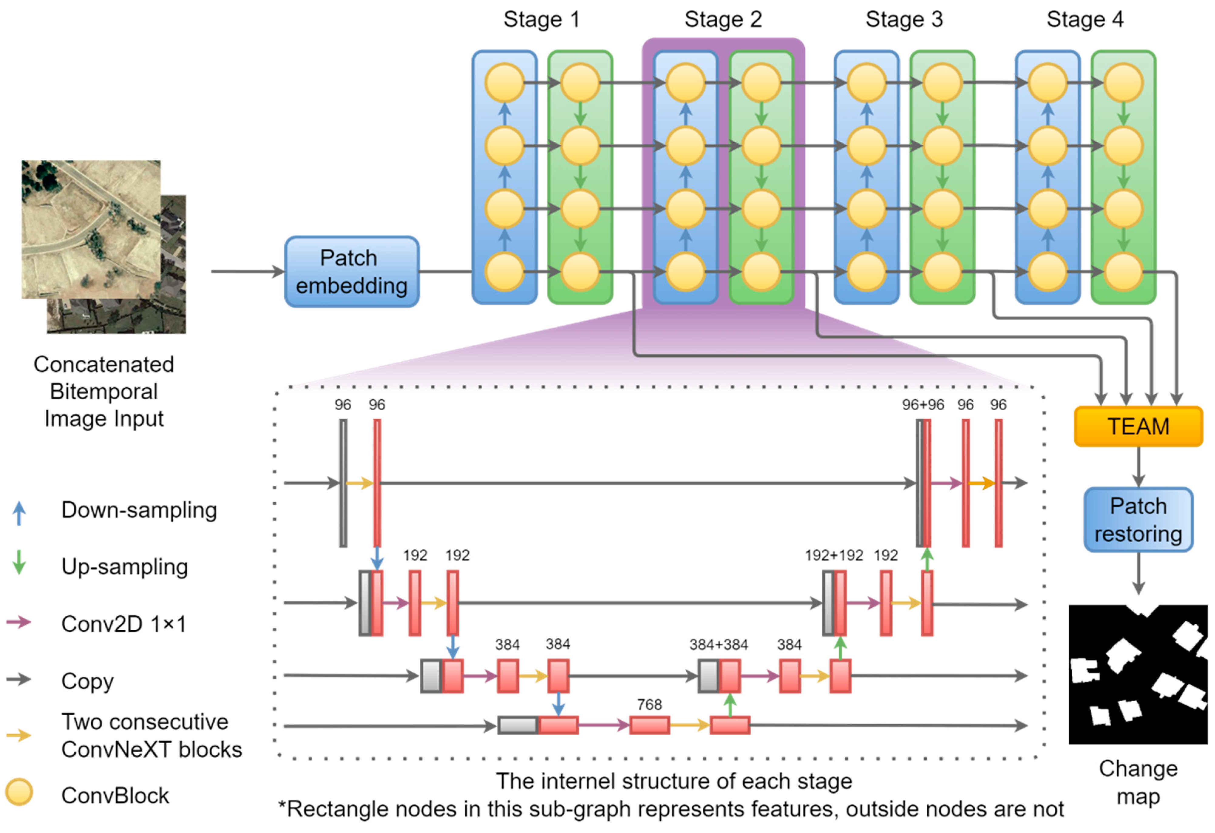
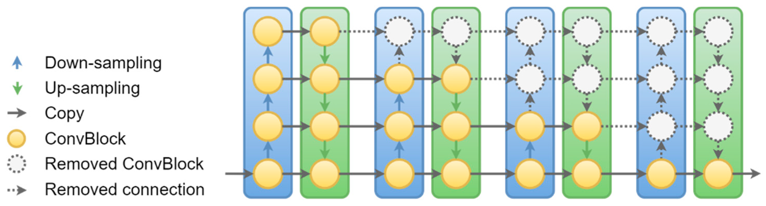
A cascaded U-Net change detection model was proposed with ConvNeXT blocks, and with the help of a patch embedding layer more U-Nets can be cascaded.

(2)

A novel attention module was proposed to facilitate the training process of cascaded U-Nets which increases accuracy of the model without extra cost at inference time.

(3)

Extensive experiments on two change detection datasets validated the effectiveness and efficiency of the proposed method.

The rest of this paper is organized as follows. In Section 2, the overall structure of our proposed model DUNE-CD is introduced along with the proposed TEAM module and the used loss function. In Section 3, the change detection datasets used in our experiments, evaluation metrics, and the comparison methods used to evaluate our model are described. In Section 4, we show our experimental results on two datasets: LEVIR-CD and CCD. Section 5 is the discussion of the effectiveness of the cascaded stages, the improvements introduced by TEAM and other modules, and the computational costs. Lastly, the conclusion is drawn in Section 6.

2. Materials and Methods

Our proposed model is introduced in this section. First, the overall structure of the proposed cascaded network is described and the structure of our model is compared with a common U-Net. Then, the internal details of the modified U-Net are presented and the mechanism of TEAM is introduced. Finally, the loss function used to train our model is described.

2.1. Overall Structure of Proposed Neural Network

The overall structure of the proposed change detection model DUNE-CD is shown in Figure 1. DUNE-CD is composed of a patch embedding layer, several cascaded U-Net stages, a TEAM module to aggregate outputs of different stages, and a patch restore layer to produce the final change map prediction.

The bi-temporal input images are concatenated into one tensor with 6 channels. This introduces asymmetry between the pair of input images (the prediction of the model will be affected by the order of before and after images), but this effect can be reduced by swapping before and after images randomly during training. In the rest of this subsection, how DUNE-CD produces the change map prediction from the fused inputs is introduced.

Patch Embedding: First, the fused input image tensor is fed into the patch embedding layer. Small regions of the input tensor are grouped into single features by the patch embedding layer, which can increase the receptive field of the model. In our model, the size of these small regions is 4 × 4 with 6 channels (2 concatenated RGB images). Every 4 × 4 non-overlapping patches with 6 channels are embedded into one feature with 96 channels. Then, these embedded features are fed into the following cascaded U-Net structure. A larger patch size can reduce the size of the input feature of the subsequent cascading structure and increase the receptive field even more; however, the predicted change map of models with a larger patch size will contain more artifacts and the cascaded structures make the model less dependent on the patch embedding layer to increase the receptive field.

Cascaded U-Net Structure: The embedded features from the patch embedding layer are then fed into the following cascaded U-Net structure. As shown in Figure 1, the cascaded U-Net structure is composed of four U-Nets. All the U-Net stages share the same structure. Each U-Net stage is composed of encoders (represented as blue rectangles in Figure 1) and decoders (represented as green rectangles). The difference between encoders and decoders is in the vertical path: in encoders, the vertical path goes upward which indicates the features are upsampled, and in decoders, the vertical path goes downwards which indicates downsampling.

The commonly used U-Net can be viewed as a single pair of encoder and decoder, compared with four pairs in our proposed network. The U-Net structure is modified to cascade different stages; in a regular U-Net the decoder has only one output. Different levels of the intermediate features of U-Nets are passed to cascade the model. To receive those multiple inputs, a 1 × 1 convolutional layer was added (shown as a purple arrow in the subgraph of Figure 1) to combine the input and internal features of encoders and decoders. Note that to align with the traditional depiction of a U-Net, the sub-graph is upside down compared with the four stages above the sub-graph.

Except for the multiple inputs and outputs, another small modification in the internals of U-Net is introduced. The channel sizes are changed when upsampling or downsampling compared with the original U-Net which modifies channel sizes in convolution layers. As channel sizes are changed only in the downsampling layer of ConvNeXT, we follow a similar approach and change channel sizes only in downsampling and upsampling layers. This modification makes the model slightly easier to implement because channels are changed in the upsampling layers and downsampling layers, and the input shape and output shape of ConvNeXT layers are kept the same. Thus, the input can be directly added to the output as a residual connection. Two subsequent ConvNeXT layers are used in each level (the yellow arrow in the subgraph of Figure 1), which are similar to two consecutive 3 × 3 convolutional layers often used in regular U-Nets.

The complex skip connections rules used by many previous works between each stage are not necessary with the help of built-in residual connections inside the ConvNeXT blocks and our proposed attention mechanism. These U-Net stages, which can receive multiple inputs and outputs, are cascaded together directly. The patch embedding layer produces embedding with a channel size of 96 which is used as the input of the cascaded structures.

TEAM Module: The outputs of each stage are fed into our proposed Training whEel Attention Module (TEAM), which can be viewed as a simple weighted sum. The novelty of TEAM is that these attention weights are shifted during the training process. To make the behavior of the TEAM module more interpretable, scalar values are used as attention weights for each input of TEAM. These attention weights are updated both by gradient descent and our attention shift algorithm. At the beginning of the training process, this module provides shortcuts from the shallow stages of the cascaded structure. As training proceeds, these shortcuts are gradually removed. In another word, TEAM helps the network learn from easy to hard, which fits perfectly with the cascaded structures. The details of the attention shift algorithm are introduced in the next section.

Patch restoring: Finally, the aggregated output of TEAM is fed into the patch restore layer. This layer restores those features into the patches and the restored patches form the final prediction of the change map. This layer restores every feature with 96 channels to 4 × 4 patches with 2 channels (for change and non-change classes). Then, the final output can be used in training and inference.

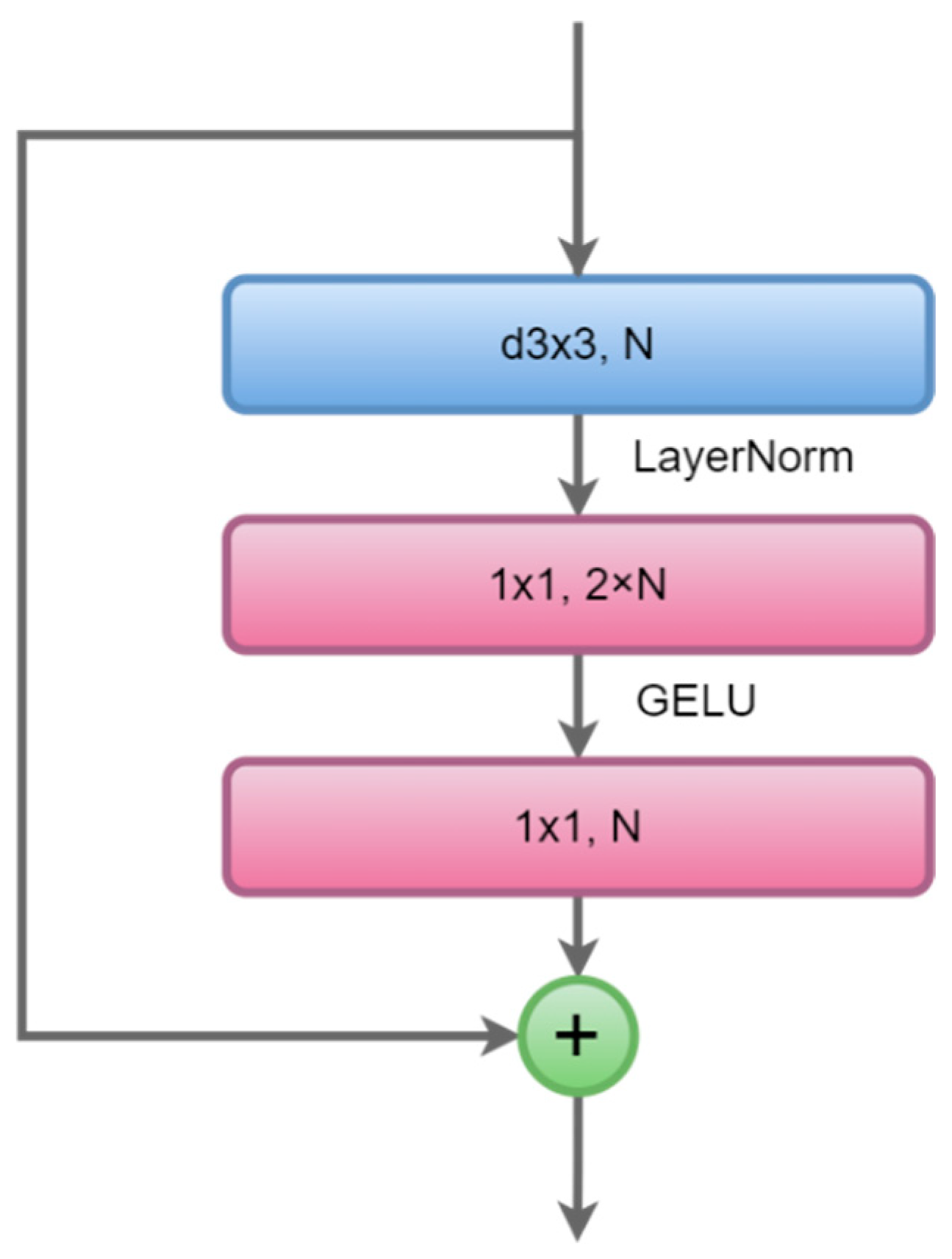
2.2. Details of Proposed Neural Network

In this subsection, the details of our proposed DUNE-CD are introduced from top to bottom. First, the internals of encoders and decoders are introduced, which are the building blocks of DUNE-CD. Then, the ConvNeXT layer used in our model is described. The upsampling and downsampling layers in the encoders and decoders are described. Next, the details of the patch embedding layer and patch restoring layer are given.

Encoder/Decoder: Each U-Net stage is composed of one pair of encoder and decoder. These encoders and decoders share the same structure and are composed of ConvBlocks. The difference between encoders and decoders is the path on which the data flow. In encoders, the features are downsampled and flow from large spatial resolution (low level) to low spatial resolution (high level) and channel sizes are doubled. In decoders, the features are continuously upsampled and channel sizes are halved at every layer.

The ConvBlocks in encoders and decoders can receive one input or two inputs with the same spatial resolution and produce one output feature as shown in Figure 1. In encoders, the output of each ConvBlock is used as the output of encoders and downsampled as an intermediate feature which is used by the next ConvBlock. The decoders work the same way except features are upsampled. The intermediate features in the encoders and decoders have channel sizes of 96, 192, 384, and 768, which are changed outside ConvBlock by upsampling layers and downsampling layers. Thus, the ConvBlocks in encoders receive features of channel sizes 96, 192, 384, and 768, respectively, and output features with the same channel size. In decoders, the channel sizes are 768, 384, 192, and 96.

ConvBlock: The ConvBlocks of encoders and decoders share the same structure, which is composed of a 1 × 1 convolution layer and dual ConvNeXT blocks. The 1 × 1 convolutions are used to reduce the channel size by 1/2, which are used when receiving two inputs that are of the same shape to fuse the two inputs into one. However, these blocks do not always get two inputs so the 1 × 1 convolution is removed in the top of the encoders and the bottom of the decoders, as in sub-graph of Figure 1. The ConvBlock output features the same shape as its only input or the two inputs.

ConvNeXT block: ConvNeXT blocks are composed of a 2D depth-wise group convolution with a kernel size of 3 × 3 followed by a LayerNorm and two pointwise convolutional layers with a GELU [51] activation function in between as illustrated in Figure 2. We replace the original 7 × 7 convolutional kernels of ConvNeXT with 3 × 3 to reduce computation. Two subsequent ConvNeXT blocks are used in ConvBlock, which is similar to the original U-Net.

Upsampling layers and Downsampling layers: Downsampling layers are composed of a LayerNorm [52] and a 2D convolutional layer. Formally,

$$LN\left(Conv\left(C_{in}, C_{out}, stride=s, kernel=s\right)\right),$$

(1)

where the $LN$ represents a layer-norm and $Conv$ is a 2D convolution with input channels $C_{in}$ and output channels $C_{out}$. The stride and kernel size are both $s$, which is set to 2 in downsampling layers.

Upsampling layers are a combination of a LayerNorm and a transposed convolutional layer as:

$$LN\left(ConvTranspose\left(C_{in}, C_{out}, stride=s, kernel=s\right)\right),$$

(2)

where $ConvTranspose$ is a transposed convolution with s set to 2 which can restore the shape of the feature changed by the upsampling layer.

The convolutional layers in the downsampling layer double the channel size and in the upsampling layer, the channel size is halved by the transposed convolution layer.

Patch embedding and patch restoring layer: The patch embedding layer is the same as the downsampling layer but the convolution layer is with a kernel size of 4 and stride of 4, as in Equation (1), with $s$ equal to 4. The patch restoring layer is the same as the upsampled layers, but the stride and kernel size is 4, as in Equation (2), with $s$ equal to 4. The patch embedding layers produce features with a channel size of 96 and the channel size of the patch restore layer’s output is 2 to correspond to the change and non-change classes.

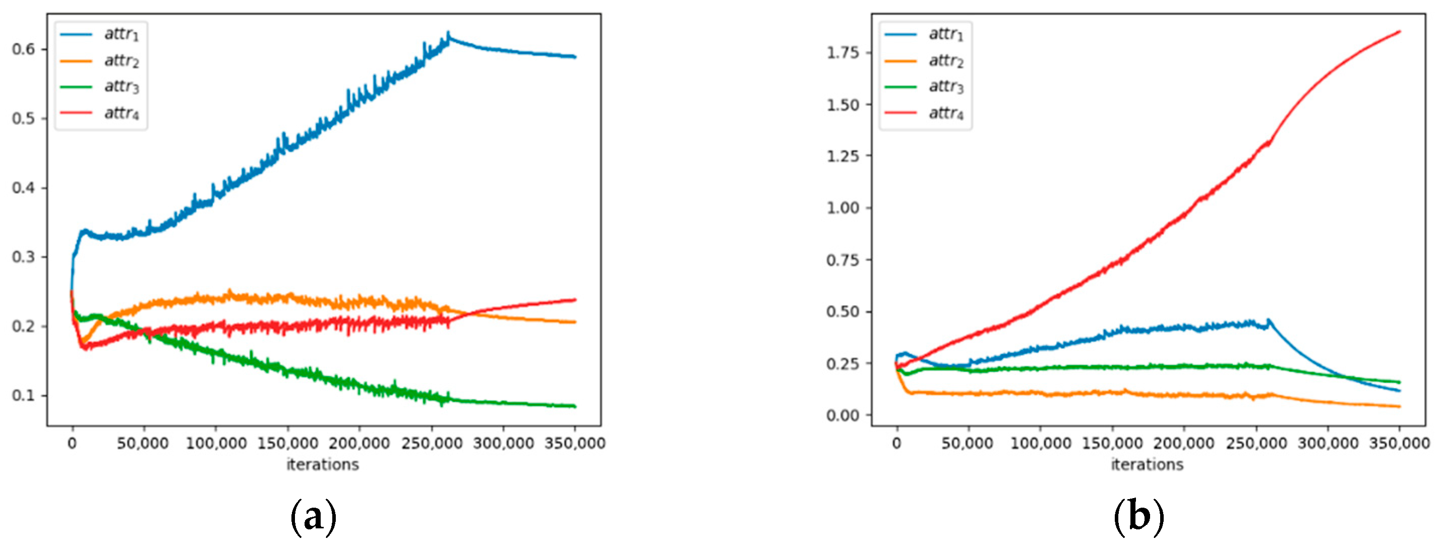
2.3. Training whEels Attention Module (TEAM)

In this subsection, the training wheels attention module (TEAM) is proposed. According to [53], the attention process can be formulated as $Attention=f\left(g\left(x\right),x\right)$, where $g\left(x\right)$ is used to generate attention which is a region to be attended and $f\left(g\left(x\right),x\right)$ is a process that combines $x$ with attention $g\left(x\right)$. However, similar to [21], $g\left(x\right)$ of our attention module is a learned weight and will not change with $x$ but is guided with prior knowledge during the training process. Besides back-prop, these weights are changed by our weight shifting policy.

The policy is based on the prior knowledge that at the beginning of training outputs from shallow stages are easier to learn, but as training proceeds, the model’s attention should be shifted to deeper stages to make more use of the cascaded structure. This is caused by the cascading nature of our network, and each U-Net’s output is dependent on the input from the previous U-Net.

To be more precise, $g\left(x\right)$ of the proposed trained shallow stage attention module is a function of trained iterations that causes the attention to shift during the training process. Perhaps this kind of training-time attention can be counted as a new paradigm of attention mechanisms. TEAM can be viewed as a simple weighted sum as follows:

$$y={\displaystyle \sum }_{\mathrm{i}=1}^{\mathrm{m}}att{r}_i{x}_i ,$$

(3)

where $\mathrm{m}$ is the number of stages, $att{r}_i$ is i-th weight, and $x_i$ is the output of the i-th stage.

The prior knowledge to be added to our model is that the desired distribution of these weights should hold this order: $att{r}_i>att{r}_{i-1}$ for all $i>1$, which ensures that deep stages are paid more attention. The simplest implantation to reduce attention on the shallow part is achieved by adding an L2 norm of weights as a regularization term of loss with a different coefficient which is large on the weights of the shallow part. This approach does not work well because these weights are trainable parameters and lower weights of the shallow parts by regularization will also reduce the weights of deeper parts of the networks and the distribution of weights will not change as desired. The attention should be shifted to the deeper stages of the network. To obtain this desired behavior, we directly modify these weights on each forward pass during the training phase.

These weights are updated with the following algorithm (Algorithm 1) described in pseudocode at every forward pass at the training phase:

Algorithm 1: Weight shifting strategy of TEAM
1.	Input:$att{r}_1^t,att{r}_2^t,\dots ,att{r}_m^t$ = weights of different stages, $\xi$ = initial learning rate, $\lambda$ = impact of shifting strategy
	Output:$att{r}_1^{t+1},att{r}_2^{t+1},\dots ,att{r}_m^{t+1}$ = shifted weights
2.	begin
3.	$att{r}_m^{t+1}=att{r}_m^t+{\displaystyle \sum _{i=1}^{m-1}}\xi {\alpha }_i\lambda att{r}_i^t$
4.	for$i \leftarrow 1 to m - 1$
5.	${\alpha }_i=\left(m-i+1\right)/m$
6.	$att{r}_i^{t+1}=\left(1-\xi {\alpha }_i\lambda \right)att{r}_i^t$
7.	end

The weights are reduced in all except the last one which is the weight corresponding to the deepest output and the reduced weights are added to the last weight. ${\alpha }_i$ is the weight shift coefficient. ${\alpha }_0$ is set to 1 and these coefficients are linearly decreased to 0. The coefficients are multiplied with $\xi$ (the initial learning rate) when the learning rate is reduced, which makes the $\xi$ larger comparatively; therefore, the effect of weight adjustment by TEAM will take over and the short-cuts from the shallow U-Net to the outputs will be gradually removed. The impact of the proposed algorithm can be tuned by the hyperparameter $\lambda$.

Each $att{r}_i$ is a scalar value and in this way the distribution of $att{r}_i$ on different stages can be easily observed. These $att{r}_i$ can be replaced with vectors with a size equal to the number of channels of each output stage and the update rules can work the same.

The TEAM only shifts attention during training, which means that TEAM does not introduce any computational cost at the inference phase but the impacts on the cascaded structure remain. With carefully chosen $\lambda$, which we set to 0.05 on both datasets, TEAM can improve the accuracy of the model. The $\lambda$ is an important hyper-parameter and will impact the training result. A large $\lambda$ will reduce TEAM to just use the output of the last stage and a small $\lambda$ will reduce TEAM to a simple weighted sum. Therefore, with a good selection of $\lambda$, TEAM can harness the power of both weighted sum and the deep cascaded structure.

2.4. Loss Function

The negative log likelihood loss is used in our framework, which is commonly used in classification tasks as a change detection problem is classifying pixels into change and non-change classes. The loss function is defined as:

$$loss=-\frac{1}{B\times W\times H}{\displaystyle \sum }_{i=1,j=1,k=1}^{B, W,H}{y}_{GT}{}_{ijk}\log \left(\sigma \left(y_o{}_{ijk}\right)\right) ,$$

(4)

where $\sigma \left(·\right)$ is a softmax function and $B$ is the batch size, $W$ is the width of the change map, and $H$ is the height; the loss is a mean product of the ground-truth vector $y_{GT}$ and the output vector $y_o$.

3. Experiments

This section includes details of our experiments. First, the datasets and evaluation metrics are described. Then, several current state-of-the-art (SOTA) comparison methods are introduced. Last, the detailed experimental settings including our hyper-parameter settings are introduced.

3.1. Datasets and Evaluation Metrics

3.1.1. Datasets

The experiments were conducted on two different change detection datasets, namely, LEVIR-CD [28] and CCD [54], to evaluate our model. These datasets are commonly used in recent change detection literature and are publicly available.

The LEVIR-CD dataset contains 637 pairs of remote sensing bitemporal images from Google Earth, and the ground sample distance (GSD) of these images is 0.5 m/pixel with corresponding binary-building-related change labels. The default split (training/validation/test) provided by the dataset is used, and the images are cropped in the validation set and test set into small 256 × 256 non-overlapping patches. Images in the training set are cropped into the same size by overlapping with a stride of 128. After cropping, the training set contains 21,805 pairs of image patches, the validation set contains 1024 pairs, and the test set contains 2048 pairs.

The CCD dataset contains 11 pairs of remote sensing images with GSD in the range from 0.03 m/pixel to 1 m/pixel of which 4 pairs are of size 1900 × 1000 and 7 pairs are of size 4725 × 2200. The original datasets already contain cropped images of size 256 × 256 and are divided into training/validation/test subsets. We use the original split provided in the dataset to train, validate, and test our model, which contains 10,000 non-overlapping image pairs with binary change maps in the training set, 3000 samples in the testing set, and 3000 in the validation set.

3.1.2. Evaluation Metrics

In all our experiments, the following metrics were used to evaluate the experimental results for comparison:

$$\mathrm{Precision}=\frac{\mathrm{TP}}{\mathrm{TP}+\mathrm{FP}} ,$$

(5)

$$\mathrm{Recall}=\frac{\mathrm{TP}}{\mathrm{TP}+\mathrm{FN}} ,$$

(6)

$$\mathrm{IoU}=\frac{\mathrm{TP}}{\mathrm{TP}+\mathrm{FP}+\mathrm{FN}} ,$$

(7)

$${\mathrm{F}}_1=\frac{2\times \mathrm{Precision} \times \mathrm{Recall}}{\mathrm{Precision} + \mathrm{Recall}} ,$$

(8)

where TP, TN, FP, and FN stand for the number of true positives, true negatives, false positives, and false negatives. Since the ${ \mathrm{F}}_1$-score provides a single score that considers both precision and recall, the ${ \mathrm{F}}_1$-score is used as the main evaluation index. In addition, the number of multiply–accumulate (MAC) operations and the average inference time to process one image pair are used to evaluate different methods.

3.2. Comparison Methods

To compare our proposed deep learning change detection model, state-of-the-art deep learning change detection models are chosen to compare with the proposed approach. We choose both types of change detection networks for comparison methods: CDNet [20], UNet++ MSOF [22], RDPNet [21], DeepLab V3 [55], and DeepLab V3+ [55] are all single-string networks. Double-stream change detection methods are also included: FC-Siam-Diff, FC-Siam-Conc [23], IFNet [24], DSAMNet [33], and BIT [26]. These models are described as follows:

FC-Siam-Diff and FC-Siam-Conc are two fully convolutional Siamese networks. These networks have two encoders with shared weights to extract features from bi-temporal inputs. The difference between the two networks is how the outputs from the two branches are fused. The kernel size of the convolutional layers of the two networks is 3 × 3.

CDNet is composed of contraction and expansion blocks. The contraction blocks consist of a convolution, batch normalization, ReLU, and max pooling, and the expansion blocks consist of un-pooling, convolution, batch normalization, and ReLU. Contraction and expansion layers are composed of 7 × 7 convolutional layers with 64 fixed channels.

DSAMNet is an attention metric-based network with a feature extractor and change decision module. ResNet-18 is used as the feature extractor. The change decision generates bi-temporal features and the distance between these features is used to compute the change map. The model was trained with two loss functions: batch contrastive loss (BCL loss) and dice loss.

IFNet extract features via a shared deep feature extraction network, which is VGG16. The extracted features are then fed into the deeply supervised difference discrimination network (DDN) to produce change prediction, in which multi-level deep features of raw images are fused with image difference features by attention modules.

DeepLab V3 is a semantic segmentation architecture. At the end of the encoder, it uses an atrous spatial pyramid pooling operation to handle the problem of segmenting objects at multiple scales. ResNet-50 is used as the backbone in our experiments.

DeepLab V3+ is improved upon DeepLabv3 by adding a decoder module to further refine the segmentation results. In our experiments, the ResNet-50 is used as the backbone.

UNet++ MSOF used nested and dense skip connections to fuse features from different levels with a multiple side-outputs fusion (MSOF) strategy to produce highly accurate results. The original configuration of the network in [22] is used in our experiments.

BIT tokenizes the bitemporal image inputs and feeds these tokens into the transformer encoder and decoder to produce the change map which is the absolute value of the difference between the outputted features. The original setting of BIT [26] is used in which ResNet-18 is used as the backbone.

RDP-Net concatenates the bitemporal image at the beginning of the network. The concatenated input is divided into patches and fed into several ConvMixer layers. Then, the output patches are merged into output features. For fair comparison, we did not include the efficient training strategy and edge loss in our experiments.

3.3. Experimental Details

The proposed model is implemented with the PyTorch framework. All methods in our paper are trained and evaluated on a single NVIDIA GeForce RTX 3060 GPU. Without loss of generality, the Adam [56] optimizer is used with an initial learning rate of 4 × 10⁻⁴ for training the CCD dataset and 0.002 for LEVIR-CD without weight decay. For training CCD, we initially used 200 epochs for training, which are commonly used as in [21,26]. Through experiments we found that with a longer training routine the networks achieved higher performance. Thus, we choose 280 epochs as a compromise between training time and model performance. Due to the overlapping cropping of the LEVIR-CD training set (which produces more data samples), we use 80 epochs. The learning rate is multiplied by 0.1 after 60 epochs when training LEVIR-CD and after 210 epochs for training CCD. Simple data augmentation is used, including random rotation of 0°, 90°, 180°, or 270° with a random flip. Due to memory constraints, the batch size is set to 8 and the size of input images is 256 × 256 for both datasets. For a fair comparison, all the models are trained with the same batch size.

4. Experimental Results

In this section, the experimental results on two change detection datasets, LEVIR-CD and CCD, are shown in detail. The results of our model are compared with state-of-the-art change detection models to verify the effectiveness of our proposed model.

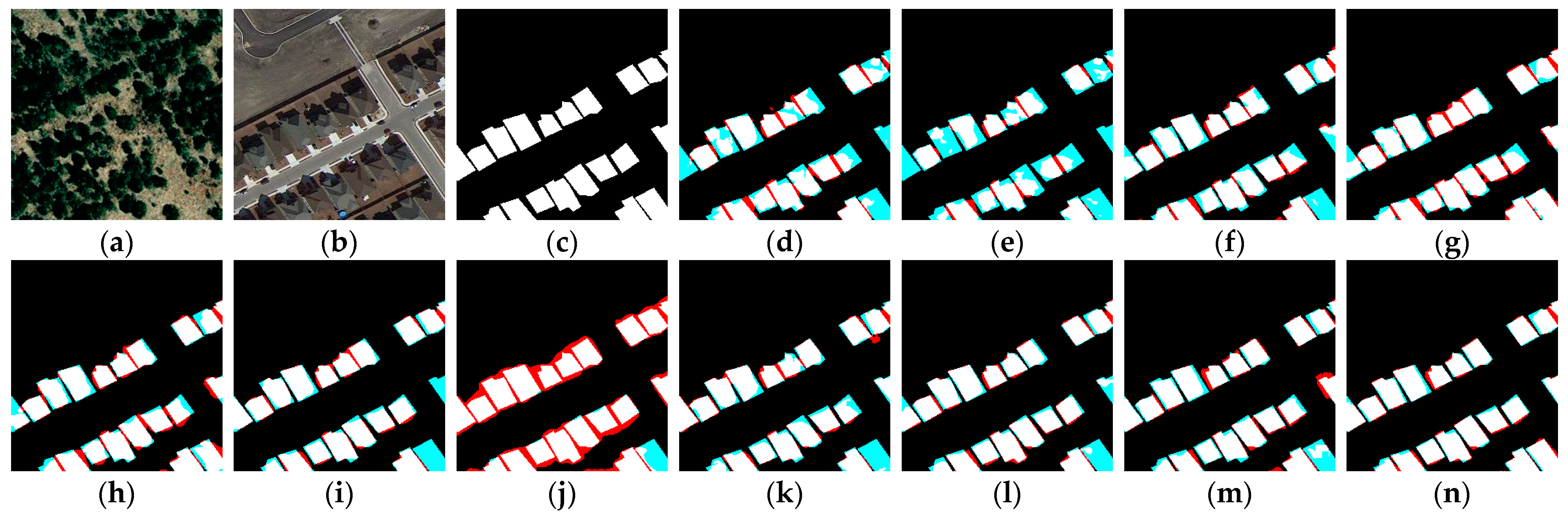
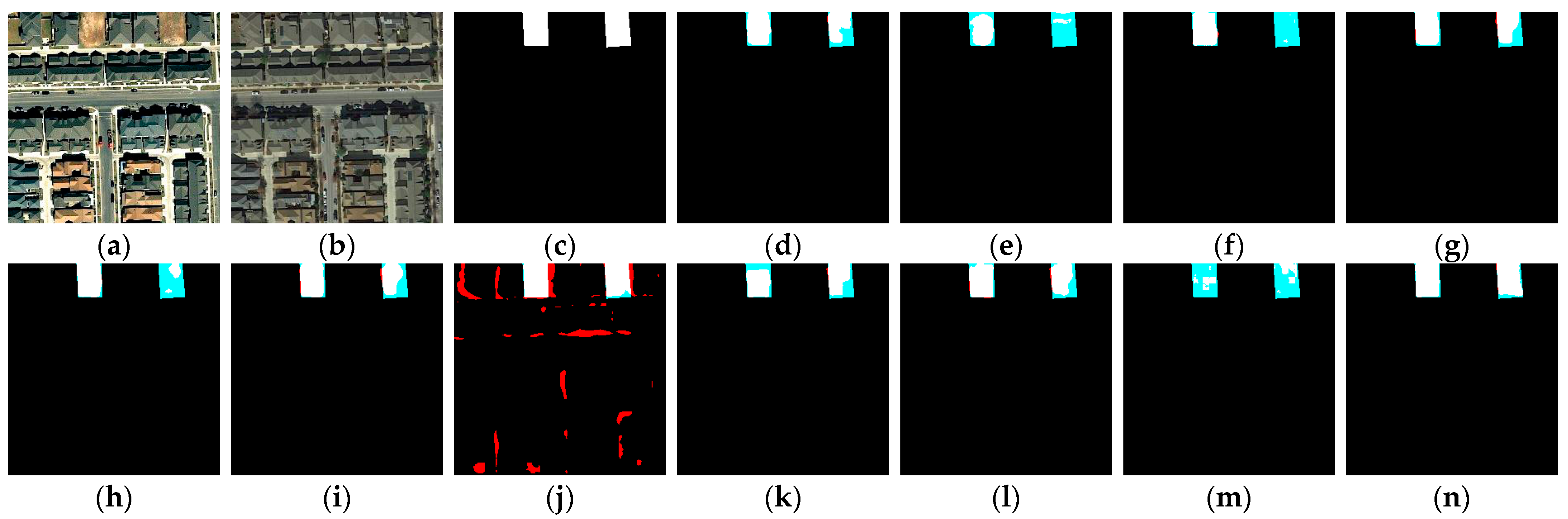
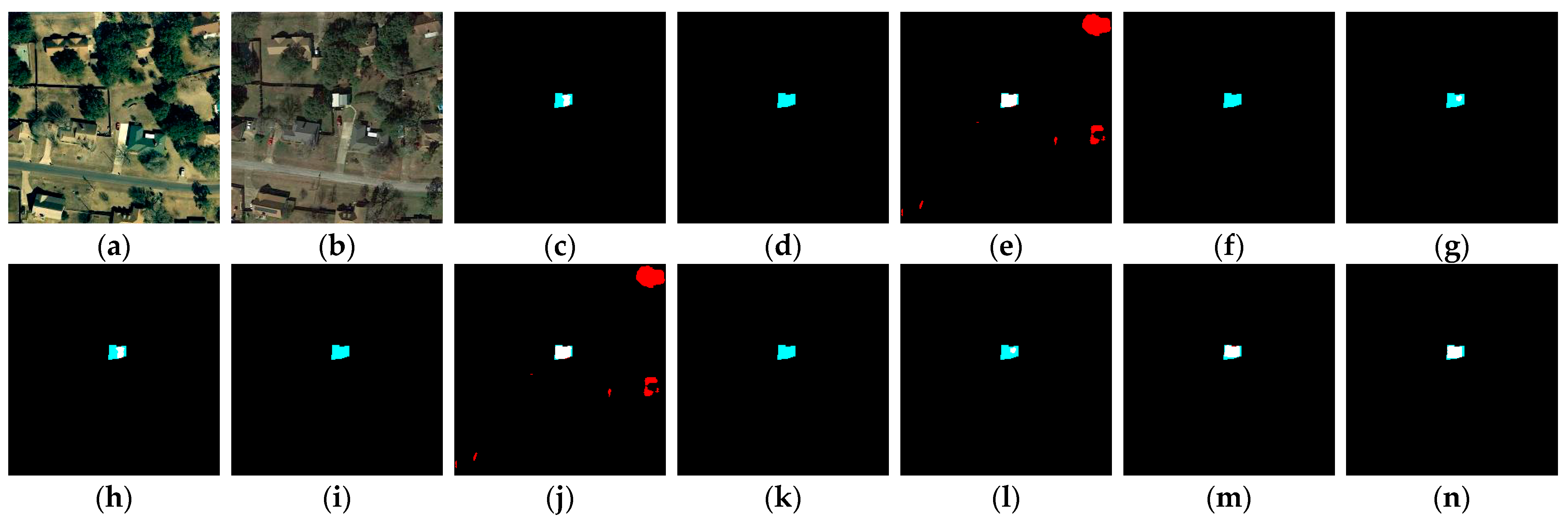
4.1. Experimental Results on LEVIR-CD

The comparison results of experiments on LEVIR-CD of our model and ten state-of-the-art change detection methods: FC-Siam-Diff and FC-Siam-Conc, CDNet, DSAMNet, IFNet, DeepLab V3, DeepLab V3+, UNet++ MSOF, BIT, and RDPNet, are shown in

Table 1. Experimental results on the LEVIR-CD dataset. The scores are described in percentage (%). The best scores are in bold font.

Methods	Precision (%)	Recall (%)	F1-Score (%)	IoU (%)	GMACs (%)	Inference Time (s)
FC-Siam-Diff	95.34	72.88	82.61	70.37	4.72	0.01680
FC-Siam-Conc	91.26	81.83	86.29	75.88	5.32	0.01713
CDNet	91.34	87.66	89.46	80.93	23.46	0.01662
DSAMNet	70.61	96.41	81.52	68.80	65.64	0.03378
IFNet	92.84	86.81	89.72	81.36	82.35	0.03298
DeepLab V3	88.77	86.03	87.38	77.59	41.15	0.02783
DeepLab V3+	90.30	86.79	88.51	79.39	43.47	0.02868
UNet++ MSOF	93.80	85.89	89.67	81.27	18.25	0.02262
BIT	92.66	88.02	90.28	82.28	8.47	0.01381
RDPNet	90.77	87.54	89.13	80.39	27.15	0.03388
DUNE-CD	92.27	88.83	90.52	82.68	25.86	0.02451

. The results show that our model obtains an F1-score of 90.52% on the LEVIR-CD dataset which is higher than all comparison methods. The precision of BIT is 92.66%, which is higher than our proposed model. The recall of DSAMNet on LEVIR-CD is 96.41%, which is higher than all other methods including our proposed method; this is due to DSAMNet being prone to predict pixels as change which drops the precision of DSAMNet to 70.61%. In change detection, the F1-score and IoU are better metrics to compare different models because these metrics encounter both precision and recall. In the F1-score and IoU, our proposed model outperformed all comparison methods. The F1-score of our model is 90.52%, which is higher than the F1-score of the second-best model, BIT, which is 90.28%.

In Figure 3, Figure 4, Figure 5 and Figure 6, the chosen results demonstrate some of the predicted change maps from DUNE-CD and compare them with FC-Siam-Diff and FC-Siam-Conc, CDNet, DSAMNet, IFNet, DeepLab V3, DeepLab V3+, UNet++ MSOF, BIT, and RDPNet for quality analysis of our algorithm. The red areas on these change maps represent false positives and the blue areas are false negatives. It shows that change maps predicted by DUNE-CD have fewer false positives and false negatives and our method can detect both small buildings (Figure 3n and Figure 6n) and large buildings (Figure 4n) well. Most mislabeling of pixels occurs around the edges of buildings, especially at corners, this is partially due to the noise in the training labels. There are more false negatives in results from BIT than DUNE-CD (Figure 3l,n, Figure 4l,n, Figure 5l,n and Figure 6l,n), which explains why BIT has a higher precision score, but the F1-score is lower than our proposed method.

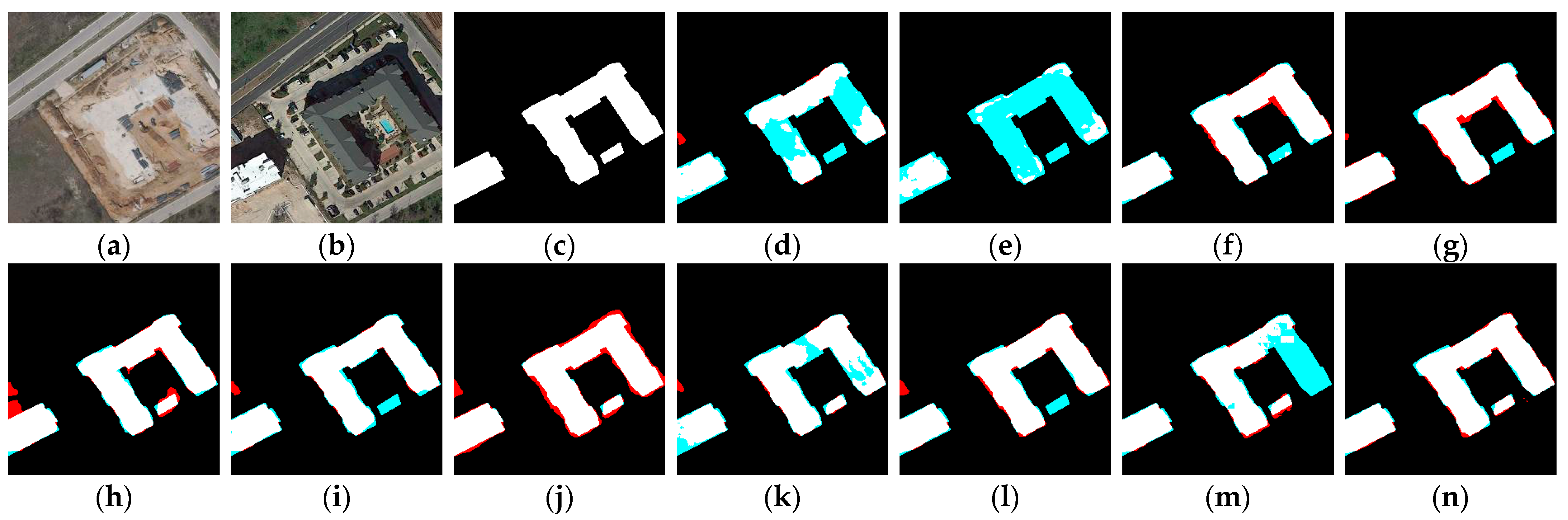
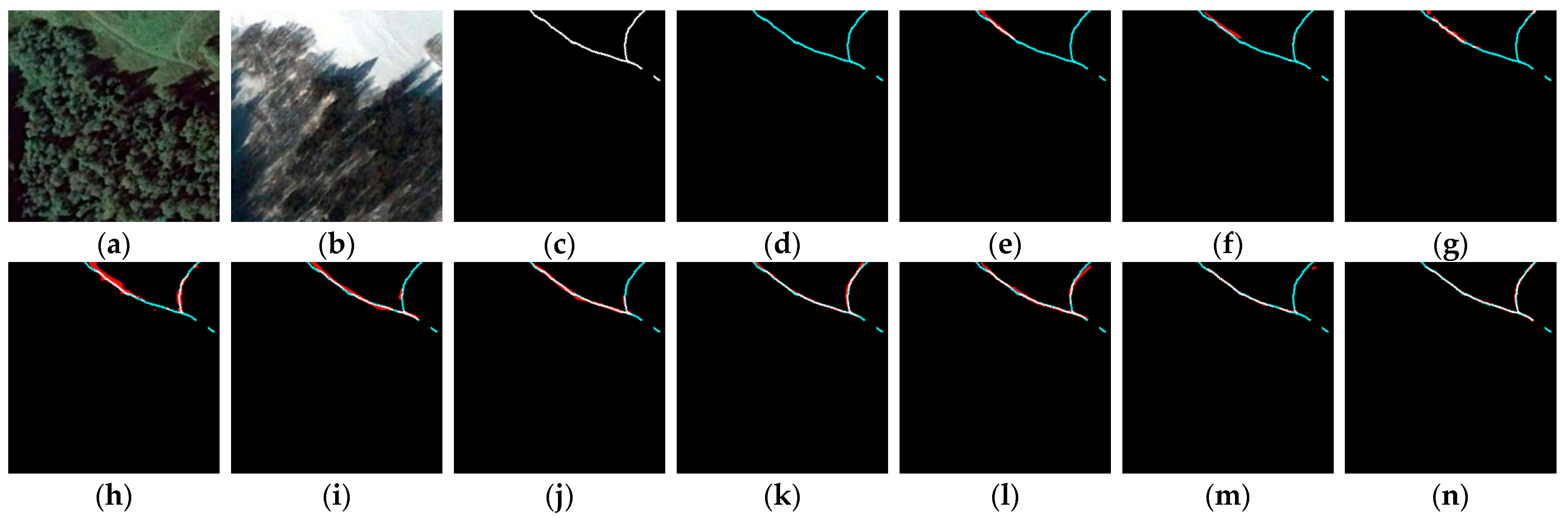
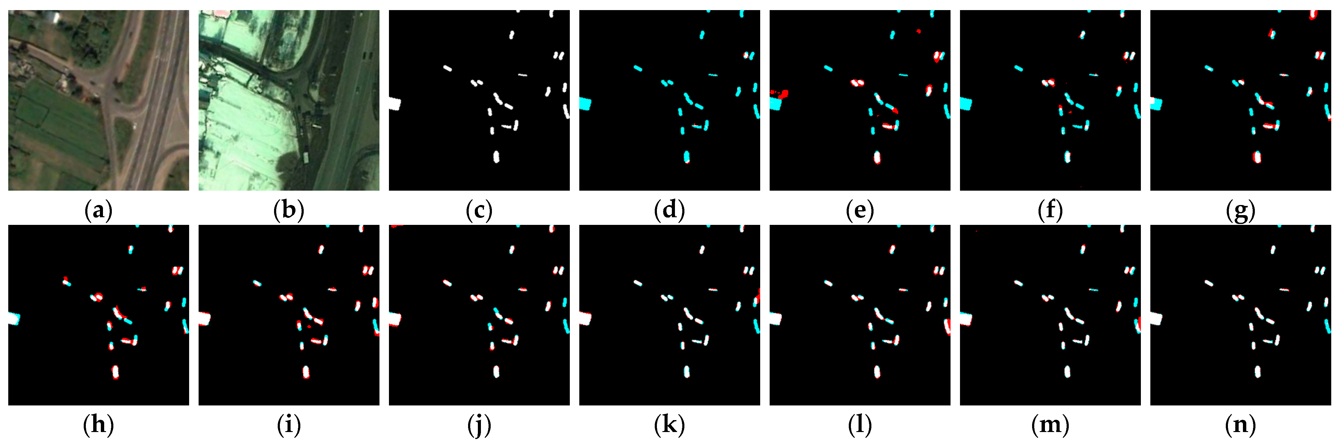
4.2. Experimental Results on CCD

In

Table 2. Experimental results on the CCD dataset. The scores are described in percentage (%). The best scores are in bold font.

Methods	Precision (%)	Recall (%)	F1-Score (%)	IoU (%)	GMACs (%)	Inference Time (s)
FC-Siam-Diff	94.56	86.43	90.31	82.34	4.72	0.01452
FC-Siam-Conc	93.63	86.69	90.03	81.86	5.32	0.01442
CDNet	95.29	88.19	91.60	84.51	23.46	0.01576
DSAMNet	97.22	95.35	96.28	92.83	65.64	0.03238
IFNet	98.71	93.25	95.90	92.13	82.35	0.03165
DeepLab V3	94.74	93.87	94.30	89.22	41.15	0.02545
DeepLab V3+	95.00	94.24	94.62	89.79	43.47	0.02640
UNet++ MSOF	96.63	94.89	95.75	91.85	18.25	0.02044
BIT	98.85	94.15	96.44	93.13	8.47	0.01285
RDPNet	99.25	94.26	96.69	93.59	27.15	0.03281
DUNE-CD	98.10	96.90	97.50	95.12	25.86	0.02451

, the F1-score of BIT is higher than RDP-Net on LEVIR-CD but lower on CCD. Our model achieves the highest F1-score on both datasets. The improvement on IoU, which is 1.53% higher than RDPNet, is more obvious than the F1-score.

To qualitatively analyze the result on CCD, some of the predicted results are shown in Figure 7, Figure 8, Figure 9 and Figure 10. The comparison shows that BIT and RDPNet can produce good detection results on CCD datasets, but our proposed model can further improve the result. Larger changed areas can be captured by almost all models (Figure 7 and Figure 8). The differences are mainly on edges (Figure 7 and Figure 8), thin roads (Figure 9), and tiny vehicles (Figure 10). Detection results of the proposed method (Figure 7n, Figure 8n, Figure 9n and Figure 10n) contain less false positives and false negatives.

5. Discussion

Though the experiments show that our DUNE-CD can outperform comparison methods, some questions are to be answered about the cascaded structure and effectiveness of TEAM. In each subsection of this section, these questions are discussed, respectively:

Q1. The DUNE-CD with four U-Net stages is tested for the comparison with the SOTA method. How will the number of cascaded stages affect the performance of DUNE-CD? What is the optimal number of stages?

Q2. How much improvement of DUNE-CD is contributed by TEAM? Are the patch embedding layer, ConvNeXT block, and the two consecutive blocks really as effective as claimed?

Q3. If a larger number of cascaded stages is good for DUNE-CD, can we further reduce the computational cost without losing advances of cascaded stages?

In Section 5.1, Q1 is answered regarding how the number of cascaded stages matters and how much improvement of model accuracy is introduced by the cascaded structure and the computational effectiveness of DUNE-CD is compared. In Section 5.2, the effectiveness of our TEAM module (Q2) on the cascaded structure is discussed and TEAM is compared with methods to produce the output. Then, ablation studies on different modules of the proposed method are discussed. In the last subsection, Q3 will be answered by cascading stages with a different number of layers at each stage, which will reduce the computational costs.

5.1. Effectiveness of Cascaded Stages

The effects of cascaded structures on CCD datasets are discussed in this section. The experimental results in

Table 3. Experimental results of models with different cascaded stages on the CCD dataset. The best scores are in bold font.

Methods	Precision (%)	Recall (%)	F1-Score (%)	IoU (%)	GMACs	Inference Time (s)
DUNE-1	99.02	94.19	96.55	93.32	6.47	0.01447
DUNE-2	99.49	94.75	97.06	94.29	12.93	0.01781
DUNE-3	99.47	94.81	97.08	94.33	19.39	0.02122
DUNE-CD	98.10	96.90	97.50	95.12	25.86	0.02451

show the performance of different cascaded stages. The DUNE-n in Table 3 means DUNE-CD with n cascaded U-Net stages, e.g., DUNE-1 is a single modified U-Net without cascading.

The performance of DUNE-CD with different numbers of stages can be quantitively analyzed from Table 3. The cascaded structure improves the performance compared with DUNE-1, which is a simple modified U-Net. Even DUNE-2 with two stages is much better than DUNE-1 with a 0.51% higher F1-score than DUNE-1. Though the performance gap between DUNE-2 and DUNE-3 is small, our proposed method with four stages achieves the best performance with a 0.15% higher F1-score than DUNE-3. The computational time increases linearly with the number of cascaded U-Nets.

The experiments showed enough evidence that the cascaded structure can improve the performance of our model. As shown in Table 3, the performance gain of cascaded stages may continue beyond four stages. However, DUNE-CD with four stages already achieves good results. As a compromise between detection accuracy and computational cost, four cascaded U-Nets are used in the proposed method.

5.2. Ablation Study

The ablation studies on the effect of TEAM on our DUNE-CD change detection model are conducted in this subsection. In the ablation experiments, TEAM with a simple weighted sum is replaced as row “DUNE-CD w/o TEAM” in

Table 4. Ablation study of TEAM on CCD dataset. The best scores are in bold font.

Methods	Precision (%)	Recall (%)	F1-Score (%)	IoU (%)	GMACs	Inference Time (s)
DUNE-CD w/o TEAM	99.47	94.71	97.03	94.24	25.86	0.02441
DUNE-CD w/o weighted sum	99.22	94.41	96.75	93.71	25.86	0.02437
DUNE-CD	98.10	96.90	97.50	95.12	25.86	0.02451

. In “DUNE-CD w/o weighted sum” the output of the last U-Net is used directly as output without the weighted sum. As shown in Table 4 below, without TEAM, only the proposed model achieves an F1-score of 97.03%. Though this is already higher than compression methods, with the help of TEAM, the F1-score is raised to 97.50%. With the weighted sum removed, the model only achieves an F1-score of 96.75%, which is the worst score. Furthermore, the number of GMACs and the inference time of all three methods are almost the same, which indicates the cost of the TEAM mechanism at inference time is negligible.

From Figure 11, it can be observed that with the help of TEAM, more attention is paid to the last stage and attention on the first three stages drops gradually. Furthermore, at the later stage of training, the curve became smoother due to learning rate scheduling, which makes the impact of TEAM greater; thus, $att{r}_1$ is dropped as shown in Figure 11b.

The results of ablation studies on the patch-embedding layer (PE), ConvNeXT blocks (CX), and two consecutive blocks (2C) are shown in

Table 5. Ablation studies of patch-embedding layer (PE), ConvNeXT blocks (CX), and two consecutive blocks (2C) on the CCD dataset. The best scores are in bold font, and the module is enabled when checked with “✓”.

Method	Modules			Metrics				GMACs	Inference Time (s)
	2C	PE	CX	Precision (%)	Recall (%)	F1-Score (%)	IoU (%)
Baseline	-	-	-	84.91	65.85	74.18	58.95	65.74	0.029
Proposed 1	-	-	✓	97.37	96.08	96.72	93.65	61.22	0.043
Proposed 2	-	✓	✓	97.33	95.42	96.37	92.99	4.04	0.012
DUNE-1	✓	✓	✓	99.02	94.19	96.55	93.32	6.47	0.013

below. All these methods removed the TEAM module and experimented with a single U-Net. The “Proposed 1” is a U-Net with ConvNeXT blocks. The ConvNeXT blocks increased the F1-score significantly compared with the baseline method. However, the computational time is very slow. With patch embedding, “Proposed 2” is four times faster than “Proposed 1” with a slight drop in the detection accuracy. The spatial size of the features is reduced via patch embedding; thus, the increase in inference time by the two consecutive blocks is trivial. Furthermore, our proposed method with four cascaded U-Nets achieves higher scores with half the computational time compared with “Proposed 1”.

5.3. More Efficient Cascaded Stages

The main disadvantage of the cascading structure is the time and memory complexity. Each stage must be executed after all previous stages are finished, and the final output is produced following an up and down path across different stages. The memory usage and inference time grows linearly with the number of cascaded stages but the performance gain does not. In real-world change detection, application data are often processed offline and thus time complexity is not critical in these applications. The computational cost of the cascaded U-Nets is reasonable.

To partially overcome this difficulty. In this subsection, we discuss a method to reduce the computational costs but still harness the power of cascaded structures. In our proposed method, we cascaded U-Nets with the same levels. Further experiments indicate that if the upper right part of the proposed model is removed, the model can almost half the computational cost with a slight loss in accuracy. The reduced cascaded U-Net structure is shown in Figure 12.

The experimental results of the reduced U-Net structure are shown in

Table 6. Experimental results of the reduced model on the LEVIR-CD dataset. The best scores are in bold font.

Methods	Precision (%)	Recall (%)	F1-Score (%)	IoU (%)	GMACs	Inference Time (s)
DUNE-CD	92.27	88.83	90.52	82.68	25.86	0.02451
DUNE-CD (Reduced)	91.74	88.74	90.22	82.18	15.40	0.01950

and

Table 7. Experimental results of the reduced model on the CCD dataset. The best scores are in bold font.

Methods	Precision (%)	Recall (%)	F1-Score (%)	IoU (%)	GMACs	Inference Time (s)
DUNE-CD	98.10	96.90	97.50	95.12	25.86	0.02451
DUNE-CD (Reduced)	99.61	94.89	97.19	94.54	15.40	0.02196

. With a slight loss in accuracy, the model can be reduced to almost half the size. It can be seen from Table 6 that the reduced model achieves an F1-score of 97.19% on the CCD dataset and can also achieve a decent performance in the LEVIR-CD dataset. This reduced model’s prediction result is more accurate than the proposed method with three cascaded U-Nets with fewer GMACs.

6. Conclusions

In this paper, an effective change detection model with four cascaded U-Nets is proposed. The TEAM module is added to aggregate results from four cascaded stages. The proposed model DUNE-CD achieves a good result in two different change detection datasets. In the discussion part, the effectiveness of the cascaded structures by comparing models with a different number of cascaded stages is studied. Moreover, ablation experiments on the different modules of the proposed method are performed. These experiments confirmed the validity of our proposed method. Furthermore, a scheme to reduce the computation without losing the advantage of the cascaded structures is introduced. The scheme shows that our method has a better tradeoff in terms of efficiency and accuracy than the ten comparison methods.

References

1. Mehrotra, A.; Singh, K.K.; Nigam, M.J.; Pal, K. Detection of tsunami-induced changes using generalized improved fuzzy radial basis function neural network. Nat. Hazards 2015, 77, 367–381. [Google Scholar] [CrossRef]
2. Sublime, J.; Kalinicheva, E. Automatic post-disaster damage mapping using deep-learning techniques for change detection: Case study of the Tohoku tsunami. Remote Sens. 2019, 11, 1123. [Google Scholar] [CrossRef] [Green Version]
3. Bennie, J.; Duffy, J.P.; Davies, T.W.; Correa-Cano, M.E.; Gaston, K.J. Global Trends in Exposure to Light Pollution in Natural Terrestrial Ecosystems. Remote Sens. 2015, 7, 2715–2730. [Google Scholar] [CrossRef] [Green Version]
4. Chen, H.; Hua, Y.; Ren, Q.; Zhang, Y. Comprehensive analysis of regional human-driven environmental change with multitemporal remote sensing images using observed object-specified dynamic Bayesian network. J. Appl. Remote Sens. 2016, 10, 016021. [Google Scholar] [CrossRef]
5. Khan, S.H.; He, X.; Porikli, F.; Bennamoun, M. Forest Change Detection in Incomplete Satellite Images with Deep Neural Networks. IEEE Trans. Geosci. Remote Sens. 2017, 55, 5407–5423. [Google Scholar] [CrossRef]
6. Solé Gómez, À.; Scandolo, L.; Eisemann, E. A learning approach for river debris detection. Int. J. Appl. Earth Obs. Geoinf. 2022, 107, 102682. [Google Scholar] [CrossRef]
7. Chen, X.L.; Zhao, H.M.; Li, P.X.; Yin, Z.Y. Remote sensing image-based analysis of the relationship between urban heat island and land use/cover changes. Remote Sens. Environ. 2006, 104, 133–146. [Google Scholar] [CrossRef]
8. Georg, I.; Blaschke, T.; Taubenböck, H. A Global Inventory of Urban Corridors Based on Perceptions and Night-Time Light Imagery. ISPRS Int. J. Geo-Information 2016, 5, 233. [Google Scholar] [CrossRef] [Green Version]
9. Lyu, H.; Lu, H.; Mou, L.; Li, W.; Wright, J.; Li, X.; Li, X.; Zhu, X.X.; Wang, J.; Yu, L.; et al. Long-term annual mapping of four cities on different continents by applying a deep information learning method to Landsat data. Remote Sens. 2018, 10, 471. [Google Scholar] [CrossRef] [Green Version]
10. Liu, S.; Marinelli, D.; Bruzzone, L.; Bovolo, F. A Review of Change Detection in Multitemporal Hyperspectral Images: Current Techniques, Applications, and Challenges. IEEE Geosci. Remote Sens. Mag. 2019, 7, 140–158. [Google Scholar] [CrossRef]
11. Bruzzone, L.; Prieto, D.F. Automatic analysis of the difference image for unsupervised change detection. IEEE Trans. Geosci. Remote Sens. 2000, 38, 1171–1182. [Google Scholar] [CrossRef] [Green Version]
12. Deng, J.S.; Wang, K.; Deng, Y.H.; Qi, G.J. PCA-based land-use change detection and analysis using multitemporal and multisensor satellite data. Int. J. Remote Sens. 2008, 29, 4823–4838. [Google Scholar] [CrossRef]
13. Benedek, C.; Sziranyi, T. Change Detection in Optical Aerial Images by a Multilayer Conditional Mixed Markov Model. IEEE Trans. Geosci. Remote Sens. 2009, 47, 3416–3430. [Google Scholar] [CrossRef] [Green Version]
14. Cao, G.; Zhou, L.; Li, Y. A new change-detection method in high-resolution remote sensing images based on a conditional random field model. Int. J. Remote Sens. 2016, 37, 1173–1189. [Google Scholar] [CrossRef]
15. Lv, P.; Zhong, Y.; Zhao, J.; Zhang, L. Unsupervised Change Detection Based on Hybrid Conditional Random Field Model for High Spatial Resolution Remote Sensing Imagery. IEEE Trans. Geosci. Remote Sens. 2018, 56, 4002–4015. [Google Scholar] [CrossRef]
16. Celik, T. Unsupervised Change Detection in Satellite Images Using Principal Component Analysis and $k$-Means Clustering. IEEE Geosci. Remote Sens. Lett. 2009, 6, 772–776. [Google Scholar] [CrossRef]
17. Jian, P.; Chen, K.; Zhang, C. A hypergraph-based context-sensitive representation technique for VHR remote-sensing image change detection. Int. J. Remote Sens. 2016, 37, 1814–1825. [Google Scholar] [CrossRef]
18. Zhu, X.; Tuia, D.; Mou, L.; Xia, G.-S.; Zhang, L.; Xu, F.; Fraundorfer, F. Deep Learning in Remote Sensing: A Review. IEEE Geosci. Remote Sens. Mag. 2017, 5, 8–36. [Google Scholar] [CrossRef] [Green Version]
19. Shi, W.; Zhang, M.; Zhang, R.; Chen, S.; Zhan, Z. Change Detection Based on Artificial Intelligence: State-of-the-Art and Challenges. Remote Sens. 2020, 12, 1688. [Google Scholar] [CrossRef]
20. Alcantarilla, P.F.; Stent, S.; Ros, G.; Arroyo, R.; Gherardi, R. Street-view change detection with deconvolutional networks. Auton. Robots 2018, 42, 1301–1322. [Google Scholar] [CrossRef]
21. Chen, H.; Pu, F.; Yang, R.; Tang, R.; Xu, X. RDP-Net: Region Detail Preserving Network for Change Detection. arXiv 2022, arXiv:2202.09745. [Google Scholar] [CrossRef]
22. Peng, D.; Zhang, Y.; Guan, H. End-to-End Change Detection for High Resolution Satellite Images Using Improved UNet++. Remote Sens. 2019, 11, 1382. [Google Scholar] [CrossRef] [Green Version]
23. Caye Daudt, R.; Le Saux, B.; Boulch, A. Fully convolutional siamese networks for change detection. In Proceedings of the 2018 25th IEEE International Conference on Image Processing (ICIP), Athens, Greece, 7–10 October 2018; pp. 4063–4067. [Google Scholar] [CrossRef] [Green Version]
24. Zhang, C.; Yue, P.; Tapete, D.; Jiang, L.; Shangguan, B.; Huang, L.; Liu, G. A deeply supervised image fusion network for change detection in high resolution bi-temporal remote sensing images. ISPRS J. Photogramm. Remote Sens. 2020, 166, 183–200. [Google Scholar] [CrossRef]
25. Bandara, W.G.C.; Patel, V.M. A Transformer-Based Siamese Network for Change Detection. arXiv 2022, arXiv:2201.01293. [Google Scholar]
26. Chen, H.; Qi, Z.; Shi, Z. Remote Sensing Image Change Detection with Transformers. IEEE Trans. Geosci. Remote Sens. 2022, 60, 5607514. [Google Scholar] [CrossRef]
27. Zhan, Y.; Fu, K.; Yan, M.; Sun, X.; Wang, H.; Qiu, X. Change Detection Based on Deep Siamese Convolutional Network for Optical Aerial Images. IEEE Geosci. Remote Sens. Lett. 2017, 14, 1845–1849. [Google Scholar] [CrossRef]
28. Chen, H.; Shi, Z. A spatial-temporal attention-based method and a new dataset for remote sensing image change detection. Remote Sens. 2020, 12, 1662. [Google Scholar] [CrossRef]
29. Liu, J.; Gong, M.; Qin, A.K.; Tan, K.C. Bipartite Differential Neural Network for Unsupervised Image Change Detection. IEEE Trans. Neural Networks Learn. Syst. 2020, 31, 876–890. [Google Scholar] [CrossRef]
30. Yang, K.; Xia, G.-S.; Liu, Z.; Du, B.; Yang, W.; Pelillo, M.; Zhang, L. Asymmetric Siamese Networks for Semantic Change Detection in Aerial images. IEEE Trans. Geosci. Remote Sens. 2021, 60, 1–18. [Google Scholar] [CrossRef]
31. Liu, J.; Chen, K.; Xu, G.; Sun, X.; Yan, M.; Diao, W.; Han, H. Convolutional Neural Network-Based Transfer Learning for Optical Aerial Images Change Detection. IEEE Geosci. Remote Sens. Lett. 2020, 17, 127–131. [Google Scholar] [CrossRef]
32. Pan, J.; Li, X.; Cai, Z.; Sun, B.; Cui, W. A Self-Attentive Hybrid Coding Network for 3D Change Detection in High-Resolution Optical Stereo Images. Remote Sens. 2022, 14, 2046. [Google Scholar] [CrossRef]
33. Liu, M.; Shi, Q. Dsamnet: A Deeply Supervised Attention Metric Based Network for Change Detection of High-Resolution Images. In Proceedings of the 2021 IEEE International Geoscience and Remote Sensing Symposium IGARSS, Brussels, Belgium, 11–16 July 2021; pp. 6159–6162. [Google Scholar] [CrossRef]
34. Song, F.; Zhang, S.; Lei, T.; Song, Y.; Peng, Z. MSTDSNet-CD: Multiscale Swin Transformer and Deeply Supervised Network for Change Detection of the Fast-Growing Urban Regions. IEEE Geosci. Remote Sens. Lett. 2022, 19, 1–5. [Google Scholar] [CrossRef]
35. Zhang, C.; Wang, L.; Cheng, S.; Li, Y. SwinSUNet: Pure Transformer Network for Remote Sensing Image Change Detection. IEEE Trans. Geosci. Remote Sens. 2022, 60, 1–13. [Google Scholar] [CrossRef]
36. He, K.; Gkioxari, G.; Dollár, P.; Girshick, R. Mask R-CNN. arXiv 2017, arXiv:1703.06870. [Google Scholar]
37. Quispe, D.A.J.; Sulla-Torres, J. Automatic Building Change Detection on Aerial Images using Convolutional Neural Networks and Handcrafted Features. Int. J. Adv. Comput. Sci. Appl. 2020, 11, 679–684. [Google Scholar] [CrossRef]
38. Maiya, S.R.; Babu, S.C. Slum Segmentation and Change Detection: A Deep Learning Approach. arXiv 2018, arXiv:1811.07896. [Google Scholar]
39. Adam, A.; Sattler, T.; Karantzalos, K.; Pajdla, T. Objects Can Move: 3D Change Detection by Geometric Transformation Consistency. In Computer Vision—ECCV 2022, Proceedings of the 17th European Conference; Tel Aviv, Israel, 23–27 October 2022, Avidan, S., Brostow, G., Cissé, M., Farinella, G.M., Hassner, T., Eds.; Springer Nature: Cham, Switzerland, 2022; pp. 108–124. [Google Scholar]
40. Tan, M.; Pang, R.; Le, Q.V. EfficientDet: Scalable and Efficient Object Detection. In Proceedings of the 2020 IEEE/CVF Conference on Computer Vision and Pattern Recognition (CVPR), Seattle, WA, USA, 13–19 June 2020; IEEE Computer Society: Los Alamitos, CA, USA, 2020; pp. 10778–10787. [Google Scholar]
41. Ronneberger, O.; Fischer, P.; Brox, T. U-Net: Convolutional Networks for Biomedical Image Segmentation. In Proceedings of the Medical Image Computing and Computer-Assisted Intervention—MICCAI 2015, Munich, Germany, 5–9 October 2015; pp. 234–241. [Google Scholar]
42. Liu, H.; Shen, X.; Shang, F.; Ge, F.; Wang, F. CU-Net: Cascaded U-Net with Loss Weighted Sampling for Brain Tumor Segmentation. arXiv 2019, arXiv:1907.07677. [Google Scholar]
43. Bao, L.; Yang, Z.; Wang, S.; Bai, D.; Lee, J. Real Image Denoising Based on Multi-Scale Residual Dense Block and Cascaded U-Net with Block-Connection. In Proceedings of the 2020 IEEE/CVF Conference on Computer Vision and Pattern Recognition (CVPR), Los Alamitos, CA, USA, 14–19 June 2020; pp. 1823–1831. [Google Scholar]
44. Ma, K.; Shu, Z.; Bai, X.; Wang, J.; Samaras, D. DocUNet: Document Image Unwarping via a Stacked U-Net. In Proceedings of the 2018 IEEE/CVF Conference on Computer Vision and Pattern Recognition (CVPR), Salt Lake City, UT, USA, 18–23 June 2018; pp. 4700–4709. [Google Scholar]
45. Ghosh, A.; Ehrlich, M.; Shah, S.; Davis, L.S.; Chellappa, R. Stacked U-Nets for Ground Material Segmentation in Remote Sensing Imagery. In Proceedings of the 2018 IEEE/CVF Conference on Computer Vision and Pattern Recognition Workshops (CVPRW), Salt Lake City, UT, USA, 18–22 June 2018; pp. 252–2524. [Google Scholar]
46. Liu, G.; Li, L.; Jiao, L.; Dong, Y.; Li, X. Stacked Fisher autoencoder for SAR change detection. Pattern Recognit. 2019, 96, 106971. [Google Scholar] [CrossRef]
47. López-Fandiño, J.; Garea, A.S.; Heras, D.B.; Argüello, F. Stacked autoencoders for multiclass change detection in hyperspectral images. In Proceedings of the IGARSS 2018—2018 IEEE International Geoscience and Remote Sensing Symposium, Valencia, Spain, 22–27 July 2018; pp. 1906–1909. [Google Scholar]
48. Liu, Z.; Mao, H.; Wu, C.-Y.; Feichtenhofer, C.; Darrell, T.; Xie, S. A ConvNet for the 2020s. arXiv 2022, arXiv:2201.03545. [Google Scholar]
49. He, K.; Zhang, X.; Ren, S.; Sun, J. Deep residual learning for image recognition. In Proceedings of the 2016 IEEE Conference on Computer Vision and Pattern Recognition (CVPR), Las Vegas, NV, USA, 27–30 June 2016; pp. 770–778. [Google Scholar]
50. Simonyan, K.; Zisserman, A. Very deep convolutional networks for large-scale image recognition. arXiv 2014, arXiv:1409.1556. [Google Scholar]
51. Hendrycks, D.; Gimpel, K. Gaussian Error Linear Units (GELUs). arXiv 2016, arXiv:1606.08415. [Google Scholar]
52. Ba, J.L.; Kiros, J.R.; Hinton, G.E. Layer Normalization. arXiv 2016, arXiv:1607.06450. [Google Scholar]
53. Guo, M.H.; Xu, T.X.; Liu, J.J.; Liu, Z.N.; Jiang, P.T.; Mu, T.J.; Zhang, S.H.; Martin, R.R.; Cheng, M.M.; Hu, S.M. Attention mechanisms in computer vision: A survey. Comput. Vis. Media 2022, 8, 331–368. [Google Scholar] [CrossRef]
54. Lebedev, M.A.; Vizilter, Y.V.; Vygolov, O.; Knyaz, V.A.; Rubis, A.Y. Change detection in remote sensing images using conditional adversarial networks. Int. Arch. Photogramm. Remote Sens. Spat. Inf. Sci. 2018, XLII-2, 565–571. [Google Scholar] [CrossRef]
55. Chen, L.-C.; Papandreou, G.; Schroff, F.; Adam, H. Rethinking atrous convolution for semantic image segmentation. arXiv 2017, arXiv:1706.05587. [Google Scholar]
56. Kingma, D.P.; Ba, J. Adam: A Method for Stochastic Optimization. arXiv 2014, arXiv:1412.6980. [Google Scholar]
Figure 1. The overall structure of our cascaded U-Net change detection model (DUNE-CD). The internal stage 2 is a typical U-Net structure, which is the same for all stages.
Remotesensing 14 06361 g001
Figure 2. The internal structure of ConvNeXT blocks.
Remotesensing 14 06361 g002
Figure 3. Visual comparisons of change detection results on LEVIR-CD of dense residential buildings using different approaches: (a) image T1, (b) image T2, (c) reference change map, (d) FC-Siam-conc, (e) FC-Siam-diff, (f) CDNet, (g) DeepLab V3, (h) DeepLab V3+, (i) UNet++ MSOF, (j) DSAMNet, (k) IFN, (l) BIT, (m) RDPNet, and (n) proposed method.
Remotesensing 14 06361 g003
Figure 4. Visual comparisons of change detection results on LEVIR-CD of large-scale building using different approaches: (a) image T1, (b) image T2, (c) reference change map, (d) FC-Siam-conc, (e) FC-Siam-diff, (f) CDNet, (g) DeepLab V3, (h) DeepLab V3+, (i) UNet++ MSOF, (j) DSAMNet, (k) IFN, (l) BIT, (m) RDPNet, and (n) proposed method.
Remotesensing 14 06361 g004
Figure 5. Visual comparisons of change detection results on LEVIR-CD with small change using different approaches: (a) image T1, (b) image T2, (c) reference change map, (d) FC-Siam-conc, (e) FC-Siam-diff, (f) CDNet, (g) DeepLab V3, (h) DeepLab V3+, (i) UNet++ MSOF, (j) DSAMNet, (k) IFN, (l) BIT, (m) RDPNet, and (n) proposed method.
Remotesensing 14 06361 g005
Figure 6. Visual comparisons of change detection results on LEVIR-CD with tiny change using different approaches: (a) image T1, (b) image T2, (c) reference change map, (d) FC-Siam-conc, (e) FC-Siam-diff, (f) CDNet, (g) DeepLab V3, (h) DeepLab V3+, (i) UNet++ MSOF, (j) DSAMNet, (k) IFN, (l) BIT, (m) RDPNet, and (n) proposed method.
Remotesensing 14 06361 g006
Figure 7. Visual comparisons of change detection results on CCD of large-scale building change using different approaches: (a) image T1, (b) image T2, (c) reference change map, (d) FC-Siam-conc, (e) FC-Siam-diff, (f) CDNet, (g) DeepLab V3, (h) DeepLab V3+, (i) UNet++ MSOF, (j) DSAMNet, (k) IFN, (l) BIT, (m) RDPNet, and (n) proposed method.
Remotesensing 14 06361 g007
Figure 8. Visual comparisons of change detection results on CCD with change of large-scale vehicles using different approaches: (a) image T1, (b) image T2, (c) reference change map, (d) FC-Siam-conc, (e) FC-Siam-diff, (f) CDNet, (g) DeepLab V3, (h) DeepLab V3+, (i) UNet++ MSOF, (j) DSAMNet, (k) IFN, (l) BIT, (m) RDPNet, and (n) proposed method.
Remotesensing 14 06361 g008
Figure 9. Visual comparisons of change detection results on CCD with change of thin roads using different approaches: (a) image T1, (b) image T2, (c) reference change map, (d) FC-Siam-conc, (e) FC-Siam-diff, (f) CDNet, (g) DeepLab V3, (h) DeepLab V3+, (i) UNet++ MSOF, (j) DSAMNet, (k) IFN, (l) BIT, (m) RDPNet, and (n) proposed method.
Remotesensing 14 06361 g009
Figure 10. Visual comparisons of change detection results on CCD with change of small-scale vehicles using different approaches: (a) image T1, (b) image T2, (c) reference change map, (d) FC-Siam-conc, (e) FC-Siam-diff, (f) CDNet, (g) DeepLab V3, (h) DeepLab V3+, (i) UNet++ MSOF, (j) DSAMNet, (k) IFN, (l) BIT, (m) RDPNet, and (n) proposed method.
Remotesensing 14 06361 g010
Figure 11. Comparison between the change of a t t r i with TEAM enabled and disabled during training on the CCD dataset. (a) Plot of a t t r i with TEAM disabled on CCD. (b) Plot of a t t r i with TEAM enabled on CCD.
Remotesensing 14 06361 g011
Figure 12. Structure of reduced DUNE-CD.
Remotesensing 14 06361 g012