Article

Quantitatively Disentangling the Geographical Impacts of Topography on PM2.5 Pollution in China

1
South China Institute of Environmental Science, Ministry of Ecology and Environment, Guangzhou 510535, China
2
National Key Laboratory of Urban Ecological Environment Simulation and Protection, Guangzhou 510535, China
3
Guangdong Institute of Land resources Surveying and Mapping, Guangzhou 510535, China
4
Guangzhou Urban Renewal Planning Institute, Guangzhou 510030, China
5
School of Surveying and Land Information Engineering, Henan Polytechnic University, Jiaozuo 454000, China
*
Author to whom correspondence should be addressed.
Remote Sens. 2022, 14(24), 6309; https://doi.org/10.3390/rs14246309
Submission received: 24 October 2022 / Revised: 29 November 2022 / Accepted: 9 December 2022 / Published: 13 December 2022
(This article belongs to the Special Issue Satellite and In Situ Observations of Air Pollution)

Abstract

:
Fine particulate matter (PM2.5) pollution’s passive effects on public health have attracted a great deal of attention. Extensive studies have tried to uncover the impacts of external drivers on PM2.5 pollution variation; however, the topography’s effects on PM2.5 pollution remain poorly understood. Using annual high-resolution concentration estimates for PM2.5, this paper quantitatively disentangled the geographical impacts of topography on the PM2.5 pollution in China and quantified the mountain blocking effects on the PM2.5 pollution dispersion on a macro scale. The results show that, in China, the plains and surrounding platforms and hills tend to suffer from long-term severe PM2.5 pollution. The most polluted topography type is the plains. In comparison, regions such as high-altitude mountains and plateaus are less affected by PM2.5 pollution. Mountains have significant and evident blocking effects on the cross-regional spread of PM2.5 pollution. Generally, Level I mountains (high elevation, density and coverage mountains) provide better blocking effects than Level II (middle elevation, density and coverage mountains) mountains and Level III mountains (low elevation, density and coverage mountains). The mountains’ blocking effects begin to play an efficient role when their altitudes reach a certain value; however, the exact altitude values vary by different mountains with a value of 163 m for all typical mountains with absolute PM2.5 concentration differences between their two sides greater than 10 μg/m3. In heavily polluted areas, PM2.5 pollution may overflow where the surrounding mountains are not high enough or the mountains’ stretch breaks. This study can provide key theoretical support for air pollution modelling and regional air pollution joint prevention and control.

1. Introduction

Fine particulate matter (PM2.5) refers to particulate matter with an aerodynamic diameter equal to or less than 2.5 microns. With relatively small particle sizes, fine particles are more likely to stay longer in the air and to be transmitted remotely, which can have a considerable impact on the ecological environment and human health [1,2,3,4,5]. PM2.5 has become the fifth leading cause of death [6]. China has accounted for more than 1.25 million premature deaths each year due to long-term exposure to polluted air in 2010, accounting for about 40% of the world’s total [7]. According to the Global Burden of Disease Study 2015 (GBD 2015), the long-term exposure to ambient PM2.5 caused 4.2 million deaths worldwide, accounting for 7.6% of the global toll of mortality in 2015. PM2.5 has attracted extensive attention due to its significant adverse effects, and it has become a key object of global air pollution prevention and control as well as a relevant topic in international atmospheric environment studies.
The studies on PM2.5 pollution by science researchers around the world mainly include the exploration of pollution causes [8,9,10,11,12], the simulation of temporal changes and spatial distributions of pollutants and research on their variation characteristics [13,14,15,16,17,18], as well as the study of the environmental impacts, weather and climate impacts and health effects induced by PM2.5 pollution [4,19,20,21,22]. Studies have proven that PM2.5 pollution is inextricably linked to natural and human activity factors. For instance, meteorological factors, including temperature, precipitation, wind conditions and atmospheric pressure may influence the clustering and dispersion of PM2.5 pollutants [9,23,24,25,26,27]. Some scholars suggested that anthropogenic emission sources, such as industrial pollutant discharge and vehicle emission, are primary contributing factors of PM2.5 pollution in cities [28,29]. Furthermore, human activities, including urban expansion and urban interior landscape planning, can also have an important impact on the temporal and spatial distributions of PM2.5 [10,11,17]. Coupled with the information from spectral, meteorological, sociometric and land use, etc., various inversion models for PM2.5 concentration were developed, including remote sensing inversion models [13,14,30], deep learning and mathematic statistics models [15,16,31], hybrid models [32,33] and so on. Regarding the environmental health effects, studies have also shown that a long-term or short-term exposure to atmospheric particulates can result in a lower vital capacity and a higher morbidity due to respiratory and cardiovascular diseases in humans, which may lead to a higher outpatient rate and mortality [1,34,35,36,37,38,39,40]. Furthermore, a high concentration of PM2.5 in the atmosphere will cause many potential environmental problems, including atmospheric dimming [41], damages to cultural relics [42], growth retardation or deaths of plants and other species [43], and even affecting climate change [44]. Of course, PM2.5 pollutants are not all harmful and without benefits. For example, PM2.5 (not pollution) in the air can serve as cloud condensation nuclei, making clouds and precipitation possible, which is essential for the Earth’s hydrological cycle. Furthermore, atomization therapy and salt therapy, which are commonly used in medical treatment, use beneficial PM2.5 substances to help cure respiratory diseases [45,46].
Topography can have a great impact on the dispersion and diffusion of air pollutants by changing the meteorological conditions (such as airflow direction, air pressure conditions, precipitation distribution, etc.). For example, studies have shown that the influence of the Qingling Mountains on the meteorological field of the Guanzhong Basin is one of the main causes of the local air pollution [47]. The basin topography surrounded by mountains makes the PM2.5 pollutant hard to disperse and is responsible for the high PM2.5 in Chendu [17]. The atmospheric circulations formed between the land, the sea and the valleys in the Beijing–Tianjing–Hebei region have affected the vertical migration and distribution of the air pollutants in this region [48,49]. Such atmospheric circulations as well as the blocking effect from city constructure can also have direct or indirect impacts on the air pollution incidents in coastal areas [17,50,51,52,53,54]. Furthermore, the research by Makiko Nakata et al. revealed that, due to the blocking effects of aerosol, the mountains have kept the concentration of aerosol from increasing in Nagano Prefecture, which is located in the center of Japan’s main island [55].
By summarizing the previous studies on air pollution, we can find that there is still a lack in the quantitative analysis of topography’s geographical impacts on air pollution, especially studies on a macro scale. This makes it difficult to effectively reveal the impacts of topography on air pollution and uncover the driving mechanism behind it. Moreover, it is not conducive to establishing a joint prevention and control mechanism among air-polluted regions. Therefore, based on the topographic data and remote sensing-driven PM2.5 concentration data, this paper studies the impacts of different geographic and geomorphic conditions on the spatial heterogeneity of PM2.5 pollution in China from a geographical perspective. Specifically, this paper aims to disentangle the spatial heterogeneity of PM2.5 pollution among different types of topography; then, to quantify the mountains’ blocking effects on the dispersion of PM2.5 pollution in particular, and the underlying mechanism is also discussed. This study can provide a key theoretical foundation for air pollution modelling and prevention.

2. Materials and Methods

2.1. PM2.5 Data

The newly available high-resolution China Regional Estimates of annual PM2.5 concentrations (V4.CH.03) produced by the Atmospheric Environmental Analysis Group of Dalhousie University was used in this study [13,14]. This dataset was first estimated using the geophysical relationships between the near-surface PM2.5 concentrations and satellite aerosol optical depth (AOD) retrievals from the NASA MODIS, MISR and SeaWIFS instruments, which were simulated by the GEOSChem chemical transport model with updated algorithms. Additionally, the regional bias between estimated and ground-based annual PM2.5 concentrations predicted by the Geographically Weighted Regression (GWR) were used to subsequently calibrate the annual average of the geophysical PM2.5 estimates. V4.CH.03 provides a product with the highest spatial resolution available so far at 0.01° × 0.01°(~1 km × 1 km) and a long time span from 2000 to 2019. Validation using data from ground-based monitors shows that these long-term satellite-derived PM2.5 data have a high consistency with ground observation site data and yield excellent consistency on an annual mean basis with R2 = 0.81 and a slope of 0.90 [13,14]. Furthermore, since it has been published, this PM2.5 dataset has been widely verified for assessments of spatial and temporal patterns of PM2.5 in China and was well employed in large-scale health exposure studies [56,57,58,59]. These advantages make V4.CH.03 a good candidate for detecting PM2.5 pollution on both a national and regional scale.

2.2. Geomorphological Data

The Geomorphologic Atlas of the People’s Republic of China (1:1 million, Figure 1a) was produced by the Institute of Geographical Sciences and Natural Resources Research, Chinese Academy of Sciences, and downloaded from the Resource and Environmental Science Data Center (http://www.resdc.cn, accessed on 10 March 2022) [60]. This product is the first ever 1:1,000,000 national geomorphological atlas of China which was created with visual interpretation from Landsat TM/ETM images and SRTM-DEM, etc. It was published by the Science Press in 2009, and it provides numerical classification systems and coding systems for the types of topography across the continental China. It has been widely used in many fields, such as land and resource surveying, environmental protection, agriculture, engineering construction, disaster monitoring, etc. [61,62,63,64]. Seven basic geomorphologic types are provided in this product based on different relief amplitude levels (Table 1), and 25 more detailed geomorphologic types are classified by considering the two indices: altitude and relief amplitude levels [60]. In the present study, we did not study the impacts from relief amplitude, so only four basic geomorphologic types were used, i.e., the plains, the platforms, the hills and the mountains.

2.3. Digital Elevation Model Data

The Digital Elevation Model (DEM, Figure 1b) data at 3” resolution (~90 m) for China was downloaded from http://viewfinderpanoramas.org/dem3.html (accessed on 10 March 2022). This dataset was developed mainly based on the data collected by the 2000 Shuttle Radar Topography Mission (SRTM) by Jonathan de Ferranti [65]. Jonathan de Ferranti filled the tiles with no SRTM data. For example, some mountain and desert areas were filled using information from topographic maps, and the results were very good, i.e., the elevation data for the voids are well aligned with the SRTM data. As described by Jonathan de Ferranti [65], the resultant DEMs were much more accurate than those created by interpolation, with or without the aid of SRTM30. Further details were thoroughly documented in the above-mentioned websites.

2.4. Data of the Mountains

Herein, the data of the mountains were originated from the Distribution of Main Mountains in China (Figure 1c), which was published by the Geological Publishing House [66]. It provides Level I, II and III mountains across China. The mountain levels originated the national standard of the name and code for Chinese mountains and peaks (GB/T 22483-2008), which was set by taking into account the balance between mountain chains, the area of the mountains, the average mountain elevation, the density and significance of mountain peaks and other necessary factors [60,67,68]. The elevation, density and coverage are greater in Level I mountains than in Level II mountains and Level III mountains. This study obtained the vector results of main mountains in China after performing geometric calibration and vectorization for the data. The data were used to study the blocking effects of mountains on the spatial diffusion of the PM2.5 pollutants.

2.5. Land Cover Data

The land cover data (Figure 1d) was used to demonstrate the distributions of anthropogenic and natural emission sources of the PM2.5 pollution. The land cover dataset in China for the year of 2019 was used in this study. It was produced by Yang and Huang [69], and is the first Landsat-derived annual China land cover dataset (CLCD) on the Google Earth Engine (GEE) platform, which contains 30 m annual land cover and its dynamics in China from 1990 to 2020. The overall accuracy of CLCD is 79.31% and it outperforms the accuracy of the widely used land cover datasets nowadays [69].

2.6. Methods

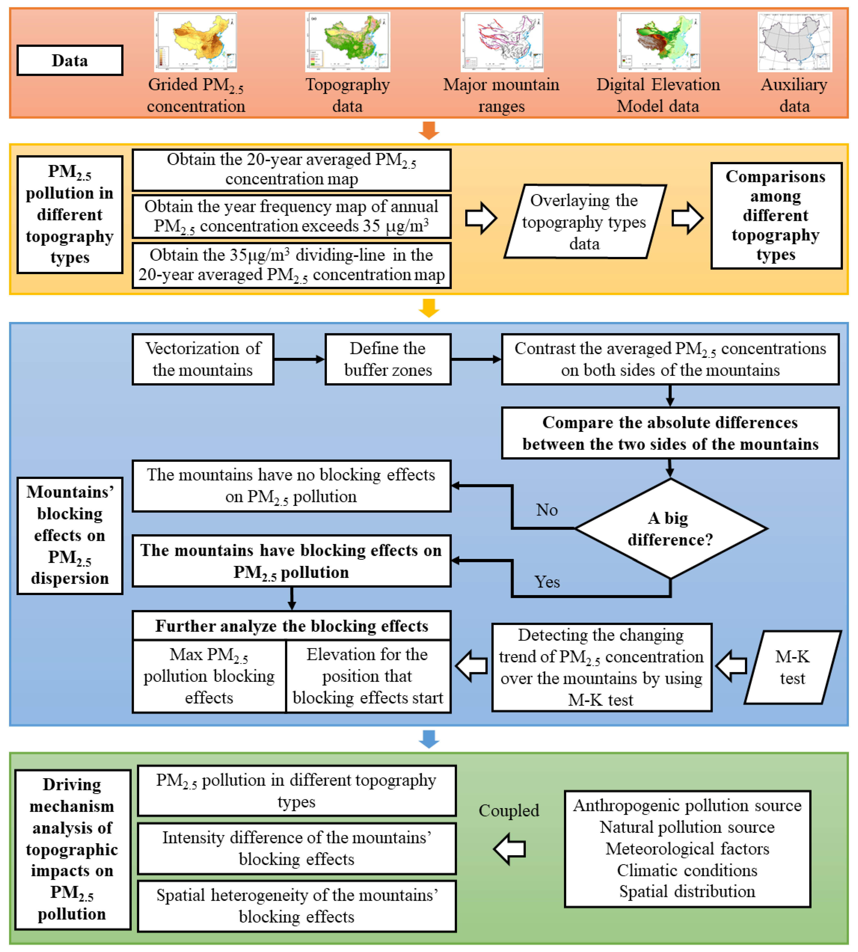
In the present study, we first compare the differences in PM2.5 pollution among different topography types by overlaying the topography types data and PM2.5 concentration data. The mountains’ blocking effects on PM2.5 dispersion was then studied by comparing the absolute PM2.5 concentration differences between both sides of the mountains. This was followed by detecting the elevation for the position at which the mountains’ effective blocking effects begin by conducting the Mann–Kendall trend test (M-K test) with digital elevation model data and the 20-year averaged PM2.5 concentration map. Finally, the driving mechanisms behind the geographically impacts of topography on PM2.5 pollution in China were analyzed by considering multiple external factors (Figure 2).

2.6.1. Preprocessing the PM2.5 Concentrations

The PM2.5 concentrations data used in this study are at annual scale. Based on these annual data, we first obtained the 20-year mean PM2.5 concentrations to proxy the averaged PM2.5 pollution condition across China over the past two decades. This was achieved by averaging the annual PM2.5 concentrations of all years from 2000 to 2019 pixel by pixel. We then obtained the 35 μg/m3 dividing line in the resulting average PM2.5 concentration map during 2000–2019. We further obtained the spatial distribution of the year frequency of annual average PM2.5 concentrations that exceeded 35 μg/m3 during 2000–2019 over China (here and after, “exceeding frequency”).

2.6.2. Identifying the Mountains’ Blocking Effects on PM2.5 Pollution

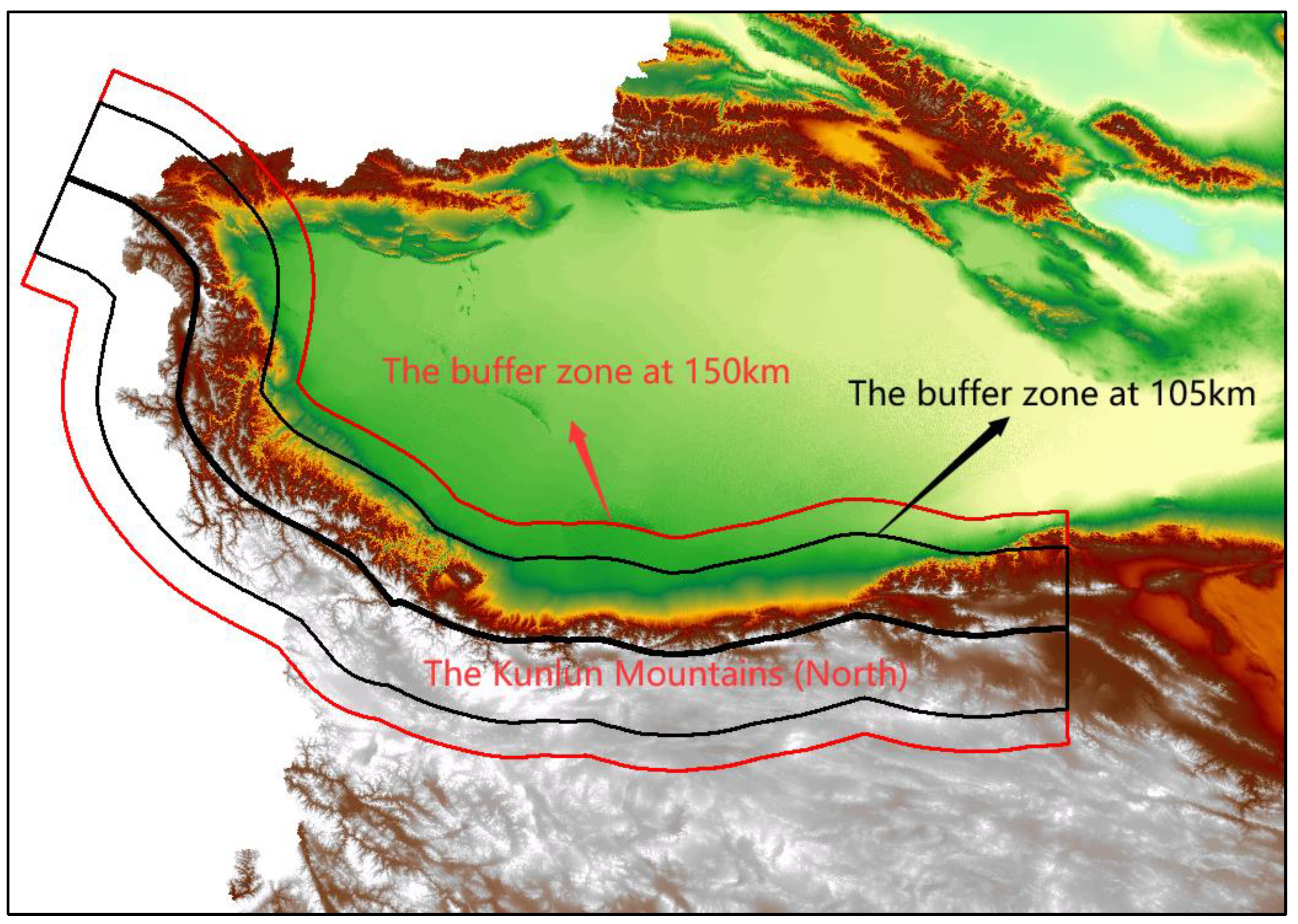
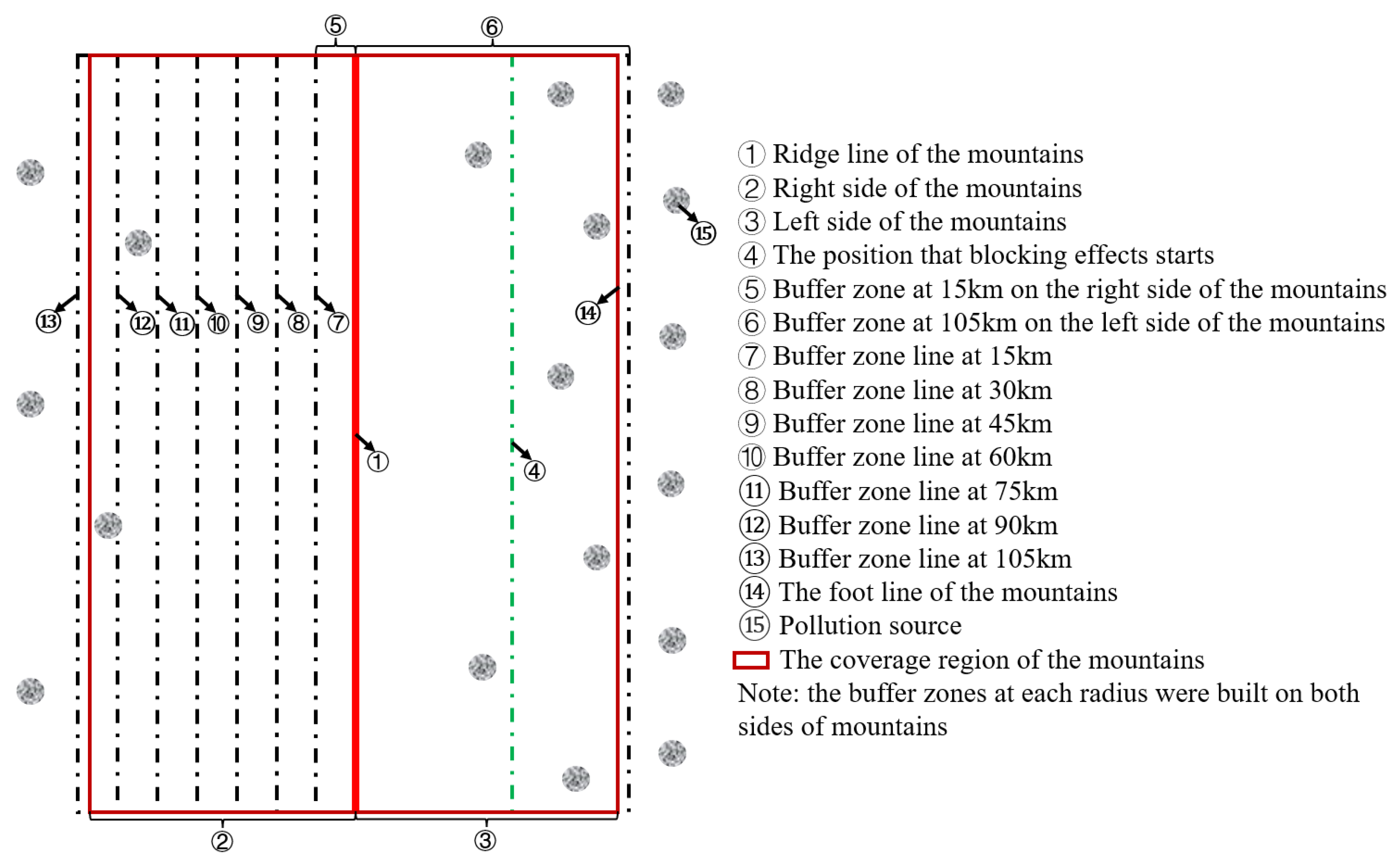
Mountains form the framework of China’s topography hinder the cross-regional spread of air pollutants, separate the spatial continuity of reginal air pollution, which leads to inconsistencies in air pollution over the left and right regions of the mountains, and form the blocking effect mentioned in this paper. This effect is a long-term, comprehensive impact that is induced by external factors, such as meteorology and emissions, on the air pollution, and specifically in this study, PM2.5 pollution. In order to identify the mountains’ blocking effects on PM2.5 pollution (Figure 2), we first contrasted the averaged PM2.5 concentration on each side of the mountains, and the absolute difference of the averaged PM2.5 concentrations was then obtained to represent the mountains’ blocking effects on PM2.5 pollution. This is performed based on different buffer zones on the two sides of the mountains. It is supposed that a higher absolute difference represents a greater blocking effect of the mountains on PM2.5 pollution. The buffers should be set from a small to a large one that can cover the coverage of the considered mountains and their foothills and nearby lands, and from the values and changes in the absolute differences of buffers with different radii, we may identify whether the averaged PM2.5 concentrations are significantly different and at what radius the mountains’ blocking effects are significant. To include large mountain ranges, this study took the Kunlun Mountains, the largest mountains in China, as a test by setting different buffers zones at 5, 10, 15, …, 120, 135, 150 km distances (Figure A1, Figure A2 and Figure A3). The results show that a buffer zone at 105 km is large enough to cover the coverage of the considered mountains and their foothills and nearby lands. Thereby, this study set the maximum radii of the buffer zones at 105 km. For convenience, only seven buffer zones were finally chosen with a spacing of 15 km, i.e., 15 km, 30 km, …, 105 km buffer zones (Figure A1, Figure A2 and Figure A3).

2.6.3. Mann–Kendall Trend Test

Herein, the M-K test was used to identify the changing trends of PM2.5 concentration in relation to the increases in mountains’ elevation. The M-K test is a non-parametric test that can be used to identify time-series data with consistently increasing or decreasing trends (Figure 2). The trends are represented using the positive or negative values of the statistical parameter, UFk, which is calculated by the following formula [70,71]:
U F k = S k E S k V a r S k   k = 1 , 2 , , n
In this formula, S k is the sequence made up of x (the time series) of n sample numbers, as illustrated below:
S k = i = 1 k r i , w h e r e   r i = + 1 ,   i f   r i > r j 0 , e l s e   j = 1 , 2 , , i
where U F 1 = 0, E S k , V a r S k is the mean and variance of the cumulative number   S k , as calculated by the following formula:
E S k = n n 1 / 4
V a r S k = n n 1 2 n + 5 / 72
The time-series data exhibit a downward trend when the UFk value is below 0, whereas the time-series data exhibit an upward trend when UFk value is above 0. There is no significant trend in time-series data (the trend is stable) if UFk value equals 0. When UFk value turns from positive to negative or from negative to positive, the time-series data tested will have a discontinuity point in the trend. The elevation where discontinuity point occurs is taken as the position at which blocking effects begin, if the PM2.5 concentration in the mountains’ left or right region with elevation higher than this discontinuity point shows continuous declination trends (Figure A3).

3. Results

3.1. PM2.5 Pollution in Different Topography Types

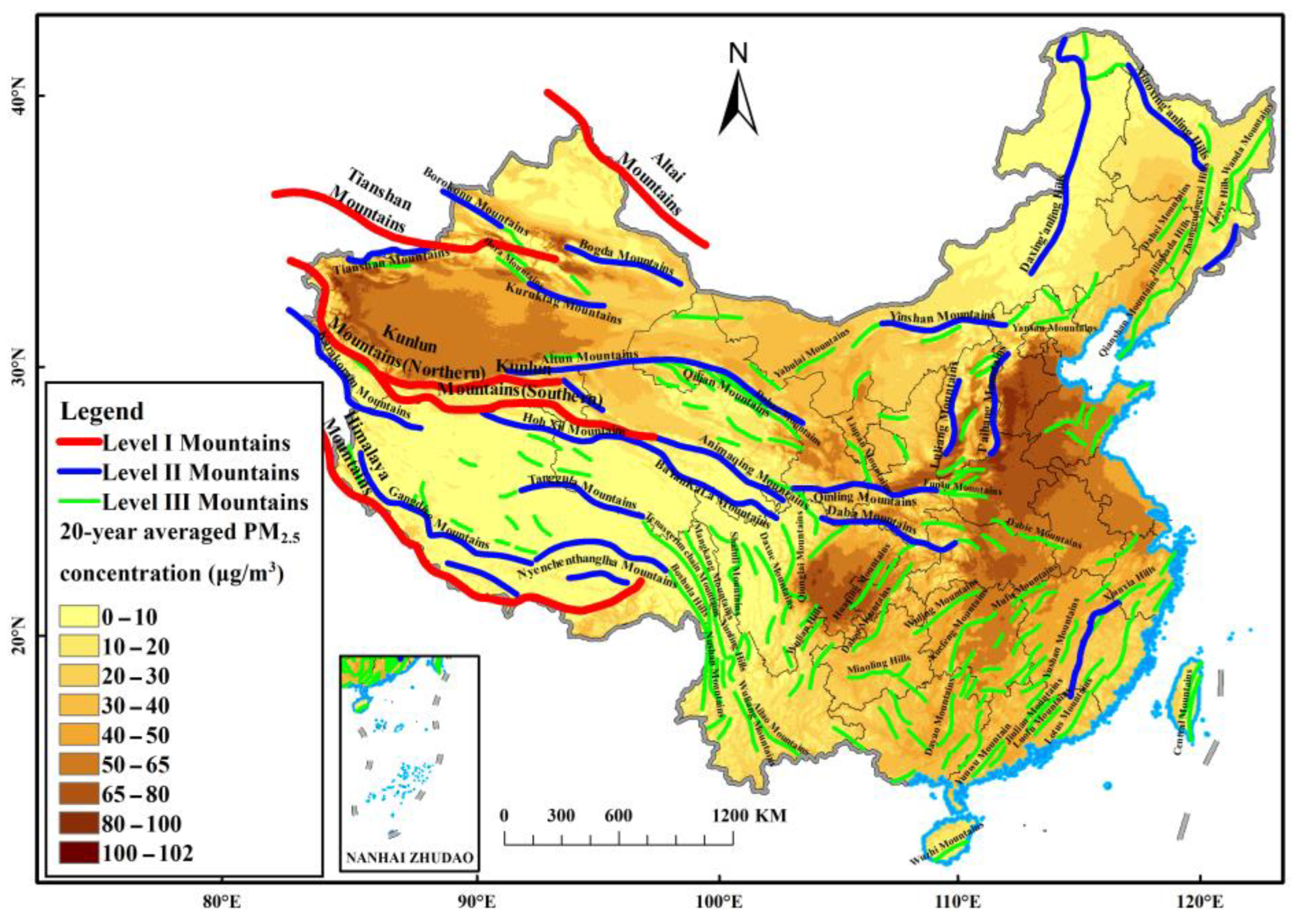
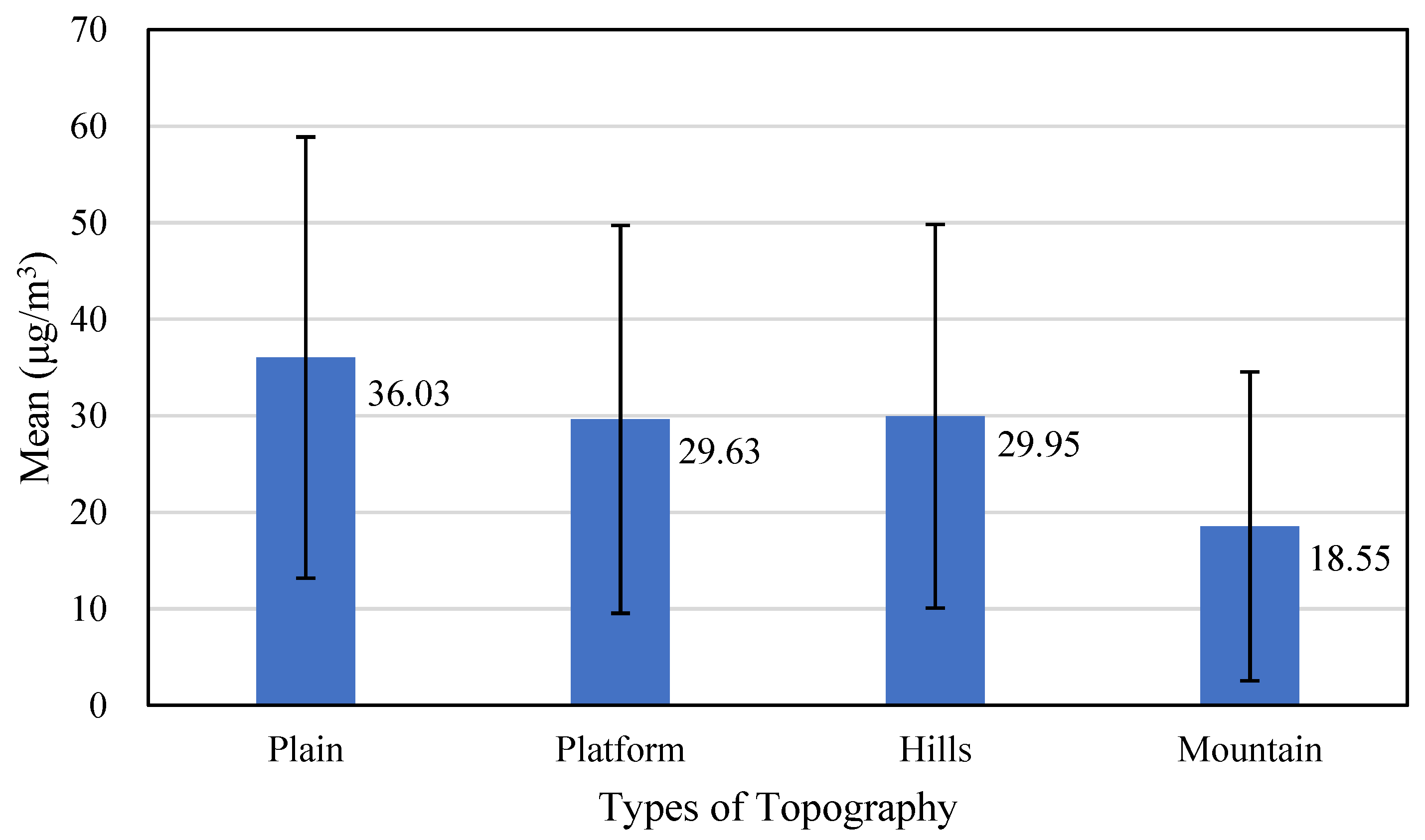
We compared the average annual PM2.5 concentrations during 2000–2019 (Figure 3) by different types of topography across China (Figure 4). The results show that plains were the most polluted geomorphology type with an average PM2.5 concentration of 36.03 μg/m3. The average PM2.5 concentrations of platforms (29.63 μg/m3) and hills (29.95 μg/m3) across China were very close to each other, which means that the nationwide PM2.5 pollution levels for these two types of topography tend to be the same. With an average PM2.5 concentration of 18.55 μg/m3, mountains are the least polluted geomorphology type in China.
We can find from the exceeding frequency map (Figure 5a) that the regions of best air quality (the light blue regions in Figure 5a) covered half of the land of China (Figure 5b), i.e., Southwest China and Northeast China, of which 54% are regions covered by mountains (Figure 5c). The regions with exceeding frequencies ranging from 1 to 15 accounted for 26.89% of the area of China (Figure 5b), where over 60% of the land surface was covered by mountains and hills (Figure 5d–f). Additionally, the heavily polluted regions with exceeding frequencies ranging from 16 to 19 covered 12.89% of the area of China (Figure 5b), in which the hills constitute the largest proportion of the land surface (as high as 38.79%, Figure 5g), while the plains and the platforms also had a considerable areal contribution (up to 36.20%, Figure 5g). The most polluted areas, i.e., the dark red regions in Figure 5a, covered 10% of the terrestrial regions of China (Figure 5b), in which the plains account for the largest proportion of the area (as high as 54.41%, Figure 5h) followed by platforms (21.00%, Figure 5h). These results indicate that PM2.5 pollution in the high-altitude mountains and hills is less severe, while the plains and the surrounding platforms and hills are more prone to suffering from long-term pollution.
We further obtained the 35 μg/m3 dividing line in the average PM2.5 concentration map during 2000–2019 (Figure 6a), and a spatial overlay analysis of this line and the topography types was then carried out to obtain the length proportion of the 35 μg/m3 dividing line across the different topography types. We can find from Figure 6a that the 35 μg/m3 dividing line encloses most of the plains and surrounding platforms and hills. The results (Figure 6b) show that the proportions of the four types of topography were 66.47% for the mountains, 13.38% for the plains, 13.22% for the hills and 6.93% for the platforms, which indicates that the mountains contributed most to the division of heavy or mild air pollution, as can be seen in Figure 3 and Figure 5a. From Figure 6c, we found that middle-elevation mountains occupied most of the proportion in the mountain regions covering the 35 μg/m3 dividing line, which plausibly implies that middle-elevation mountains may be the types of topography playing a dominating role in separating the air pollution.

3.2. Mountains’ Blocking Effects on PM2.5 Dispersion

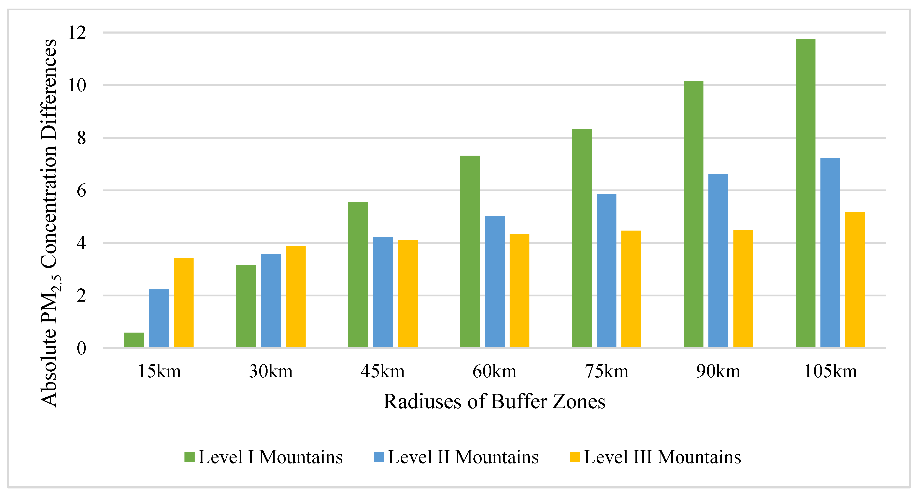
According to Figure 7, the absolute PM2.5 concentration differences between the two sides of the mountains increased with increases in the buffer zone radii. At first, such differences for Level I mountains were relatively smaller than those of Level II, and they were the largest for Level III mountains. However, as the radii of the buffer zones reached 45 km, the PM2.5 concentration differences for Level I mountains increased significantly and started to exceed Level II and Level III mountains. When the radii of the buffer zones reached 90 km, the PM2.5 concentration differences for Level I mountains were above 10 μg/m3, surpassing that for Level II and Level III mountains with absolute advantage. Similar to Level I mountains, Level II mountains had greater PM2.5 concentration differences on both sides when the radii of the buffer zones reached 45 km or greater, and such differences increased with the increase in buffer zone radii, but the change amplitude is smaller than that of Level I mountains. The PM2.5 concentration differences on both sides of Level III mountains exhibited no great change when the buffer zone radii exceeded 45 km. It can be concluded from the above results that mountains have significant blocking effects on PM2.5 concentrations, with Level I mountains’ blocking effects being greater than Level II mountains, and Level III mountains having the smallest pollutant blocking effects (Figure 7).
Nevertheless, in terms of individual mountains, the blocking effects varied greatly regarding their locations and the ambient PM2.5 pollution condition. This study chose mountains with significant blocking effects for further analysis, i.e., the PM2.5 concentration difference (absolute value) between the two sides of these mountains was significantly higher than 10 μg/m3 (hereinafter referred to as “the typical mountains”). The results show that 27 ranges of mountains were chosen (as summarized below in Table 2). When the buffer zones reached a certain radius for Level I mountains, including the Kunlun Mountains (North), Level II mountains, including the Taihang Mountains and the Tianshan Mountains, and Level III mountains, including the Huola Mountains, the Taiyue Mountains, the Longmen Mountains and the Fangdoushan Mountains, the PM2.5 pollution concentration differences were greater than 20 μg/m3. When the buffer zones reached a certain radius for Level II mountains, including the Lüliang Mountains, the Qingling Mountains and the Bogeda Mountains, and Level III mountains, including the Daqingshan Mountains and the Zhongtiao Mountains, the PM2.5 pollution concentration differences were greater than 15 μg/m3. It can be concluded from the above results that these mountains have significant blocking effects on PM2.5, and they make up the key separation belts against PM2.5 pollution.

3.3. Elevation for the Position at Which Mountains’ Effective Blocking Effects Begin

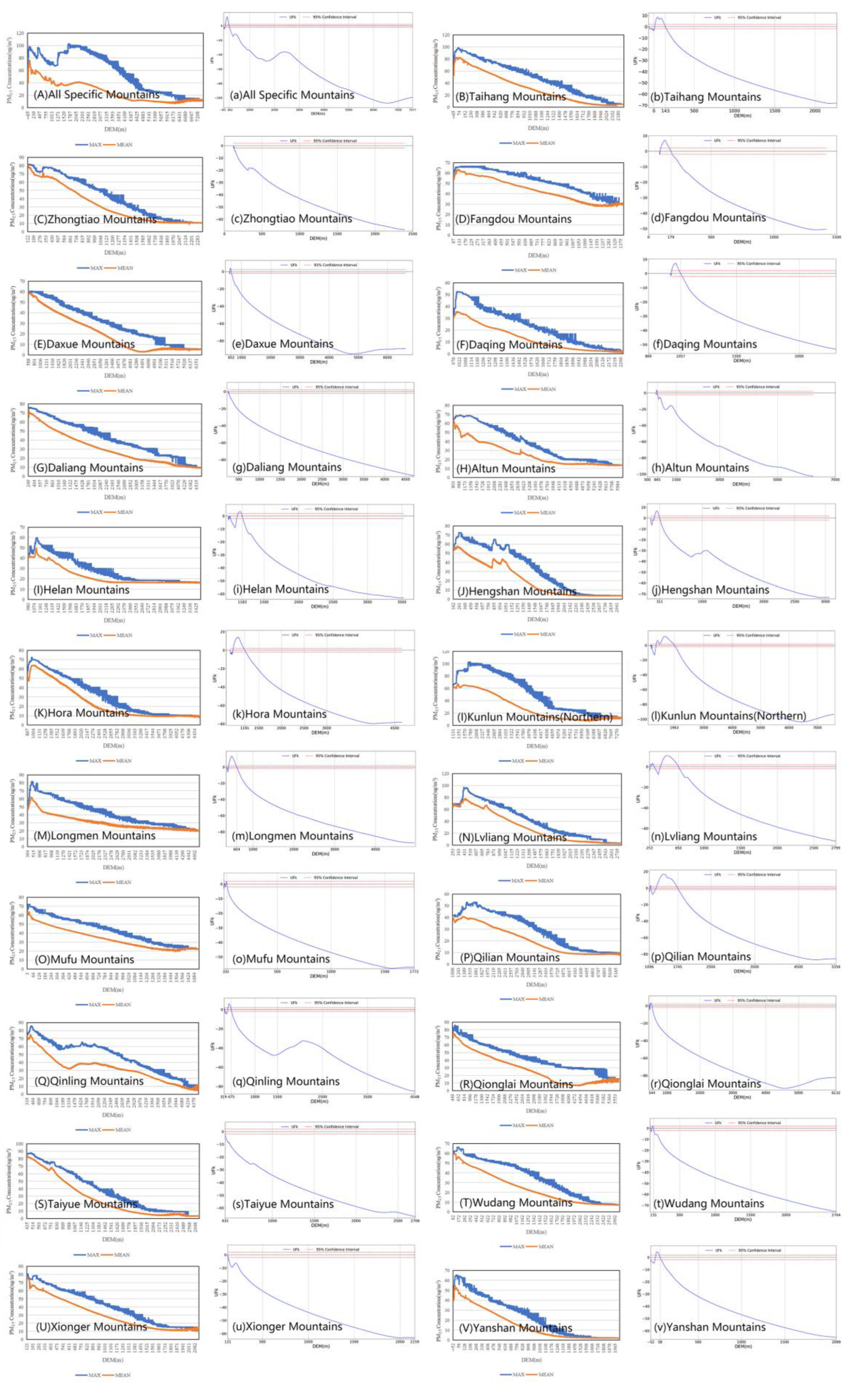
We first analyzed the trends in the PM2.5 concentrations that change with the DEM values within the 105 km buffer zone of the typical mountains mentioned in the above table. The results (Figure 8) show that the PM2.5 concentrations of Level III mountains, including the Xiong’er Mountains, the Taiyue Mountains, the Daliang Mountains and the Zhongtiao Mountains, showed falling trends immediately with the increases in elevations, while the PM2.5 concentrations of all the other typical mountains rose firstly with the increases in elevations until a certain altitude was reached. Above this altitude, a significant and sustained decline trend in PM2.5 concentrations can be observed in these mountains. This study utilized the M-K test to detect whether PM2.5 concentrations exhibited evident downtrends with increases in mountains’ elevations. As illustrated in Table 3, the results of the M-K test of all the mountains (UFk value) were dramatically lower than 0, which indicated that PM2.5 concentrations exhibited a downtrend with the increase in the mountains’ elevation.
This study further obtained the significant starting position of the mountains’ effective blocking effects (i.e., the elevation value from which the PM2.5 concentration started to have a significant and sustained decline, herein after “the starting position”) using the M-K test. Table 3 showed that in general, an altitude of 163 m was the overall significant starting position at which all typical mountains’ comprehensive effective blocking came into play, but such significant starting positions varied among different mountains. Among them, the Kunlun Mountains (North) had the highest starting position (832 m), followed by the Qilian Mountains (649 m), the Lüliang Mountains (397 m), the Mufu Mountains (329 m), the Huola Mountains (324 m), the Longmen Mountains (240 m), the Taihang Mountains (208 m), the Helan Mountains (203 m), the Qingling Mountains (156 m), the Hengshan Mountains (149 m), the Yanshan Mountains (110 m) and the rest of the mountains (below 100 m). It could be concluded that mountains have significant blocking effects on the diffusion of PM2.5.
Moreover, it can be seen from the table below that mountains had different levels of blocking effects on PM2.5 concentrations. The max PM2.5 pollution blocking effects for the Kunlun Mountains (North, Level I mountains), the Lüliang Mountains (Level II mountains), the Mufu Mountains, the Daqingshan Mountains, the Longmen Mountains, the Helan Mountains and the Fangdou Mountains (Level III mountains) are greater than 30%. For Level II mountains, including the Qilian Mountains, the Qingling Mountains, the Taihang Mountains, the Yanshan Mountains and the Hengshan Mountains (Level III mountains), have the max PM2.5 pollution blocking effects, higher than 20%. For the rest of the mountains, the max PM2.5 pollution blocking effects are below 20%.

4. Discussion

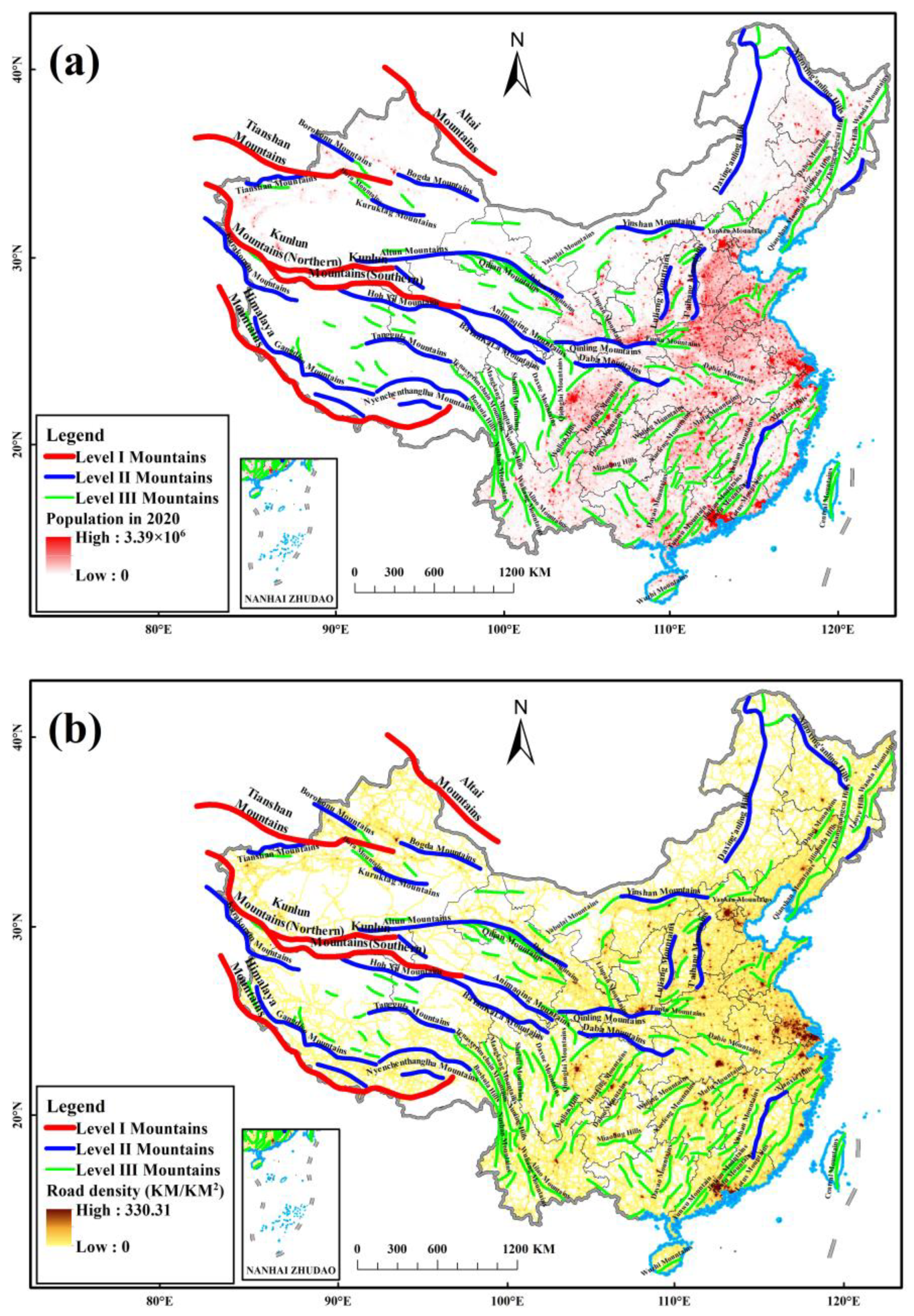
The present study showed that plains are the most polluted geomorphology type, while mountains have the least PM2.5 pollution. From the map of population counts and road density in China (Figure A4), we can find that there are much fewer human activities over the mountainous areas, and the trees in the mountains contribute to the reduction in PM2.5 pollutants [8,9]. By comparison, the geographically low-lying places, such as the North China Plain, the Guanzhong Plain and the Sichuan Basin, are vulnerable regions to haze PM2.5 pollution, mainly because there are dense pollution sources, such as urban land and farmland [17,18,39,47,49]. Moreover, significant numbers of people and roads are widespread there (Figure A4), so high-intensity air pollutants are emitted by the frequent human activities that occur there. The appearance of mountains near these places makes it difficult for emissions to spread across regions, which aggravates the cumulative effect of PM2.5 pollution over that and nearby areas. This fact, coupled with the relative quasi-stationary air condition in these low-lying places, have made these places the most polluted regions in China [8,9,72].
According to the results of Figure 3 and Figure 5, it can be seen that almost all the heavily PM2.5 polluted areas in China were encircled by high mountains, which was not conducive to the dispersion of local PM2.5 pollutants. This was consistent with the conclusions of prior studies in the Guanzhong Basin and the Beijing–Tianjin–Hebei region [47,48,49]. While preventing the cross-regional spread of air pollutants, the mountains lead to a heavy air pollution concentration in the mountain basins. For example, on the right side of the Taihang Mountains, an evident differentiation of PM2.5 pollution levels could be observed, i.e., the closer the areas to the mountains’ basins, the more serious the PM2.5 pollution would be, which could be the result of the accumulation of PM2.5 pollutants induced by the terrain–meteorological conditions near the mountains’ basins [55]. This result is supported by a previous study [72], which identified four typical weather patterns, i.e., the south-westerly winds, the north-easterly winds, the south-easterly winds and the stagnant air conditions that exist over the Beijing–Tianjin–Hebei Region, which was partially enclosed by the Yan Mountains (in the north), the Taihang Mountains (in the west) and the Dabie Mountains (in the south). The regional atmospheric circulation coupled with the influence of topography comprehensively amplified the effects of emissions by an average of 50% to 150% in the Beijing–Tianjin–Hebei region, and formed an atmospheric pollution convergence line near the foothills of the mountains. Such comprehensive effects of terrain–meteorological conditions near the upside of the Kunlun Mountains and the Altun Mountains as well as the right side of the Qionglai Mountain are also responsible for the accumulated pollution belt along these mountains. Additionally, the distance between the pollution sources and the mountains also has important influences on the distribution of PM2.5 concentrations over the mountains. For example, the urban agglomeration from Zhengzhou city to Shijiazhuang city constitutes a pollution source distribution belt in the eastern Taihang Mountains, and a heavy distribution belt of PM2.5 pollution is also seen in the mountains close to these anthropogenic sources. Similarly, in the Qinling Mountains, a heavily PM2.5 pollution area is formed over its northern part, which is near the Guanzhong urban agglomeration. Likewise, there is an accumulated pollution belt along the upside of the Kunlun Mountains, as it is near the natural emission source of the Taklimakan desert.
China is a country of varied topographical features with highlands in the west and plains in the east. The topographies in China constitute a descending three-step ladder, and these topographic features have significant effects on the atmospheric circulation of China, and further impact the diffusion of air pollutants. The research by Xu X. et al. (2015) [73] suggested that the typical topographic features of China generate a long-term clockwise vertical vortex structure on the east side of the Qinghai–Tibet Plateau, forming a sinking air flow region over the “leeward slope area” of the Qinghai–Tibet Plateau, which corresponds to the “weak wind area” on the east side of the terrain, and the combined effects of the sinking air flow and “weak wind area” are not conducive to the diffusion of air pollution emissions in industrial zones and urban agglomerations in eastern China, in particular by inhibiting the convection transport of pollutants to high altitudes, so that the east side of the Chinese plateaus presents a “south-north” belt of haze area. The mountains’ blocking effects on the dispersion of PM2.5 concentrations are controlled by prevailing winds in the lower troposphere [47,49,52,53,72], while the instantaneous effects induced by wind can finally form the overall effects induced by the composited wind direction during the last 20 years, and change the long-term topography impacts on air pollution. Central and eastern China, with their high PM2.5 levels, are the typical regions with East Asian monsoons in significant seasonal shifts of prevailing winds [49,72]. That is to say, the mountains’ blocking effects are also greatly influenced by the monsoon climate in China.
In addition, our findings show that when the mountains are located in a heavily polluted area, were not high enough or had gaps between them, the spatial overflow effects of air pollution appeared. For example, due to large gaps between the mountains or insufficient height, the PM2.5 pollutants seem to overflow through the gaps among the Level III mountains of the Wudang Mountains, the Tongbai Mountain and the Dahong Mountains (Figure A5), which means that the presence of these mountains could not effectively block the cross-regional spread of PM2.5. The overflow effects of pollution may be related to the local circulation of the mountain–valley breeze and the land–sea breeze brought by the alternation of day and night as well as the land–sea breeze resulted by the temperature pressure differences between land and sea in different seasons [50,51,52]. When the mountains are not high enough, the local circulations may transport the PM2.5 pollutants in low places across the mountains [49]. Moreover, the gaps between mountains can serve as convenient channels for transporting PM2.5 pollutants easily.
The blocking effects of the mountains depended heavily on the mountains’ level and the sizes of their buffer zones. The mountains’ level reflected their overall conditions, including the average height, coverage and density of the mountain ranges itself (i.e., the area that a mountain range covers and the number of picks within the coverage of the mountain range). When the mountains’ height, coverage and density are higher, the mountain blocking effects will be greater with less significant overflow effects of pollution, i.e., the PM2.5 concentration differences between the two sides of the mountains will be greater. In contrast, when the mountains’ height, coverage and density are lower, the mountains’ blocking effects will be smaller with significant overflow effects of pollution, i.e., the PM2.5 concentration differences between the two sides of the mountains will be smaller. Therefore, we can find that the blocking effects of Level I mountains are generally greater than that of Level II mountains, and Level III mountains’ blocking effects are relatively smaller (Figure 6, Figure 7 and Figure 8, Table 2 and Table 3). In addition, the small buffer zones may only cover the central parts of the mountains, especially for the Level I and Level II mountains (the coverage for them is generally greater than that for Level III mountains), and under this circumstance, the absolute PM2.5 concentration differences are small as the PM2.5 values tend to be the same at both sides of the central parts of the mountains. When the buffer zones began to cover the areas surrounding the mountains and are big enough to reflect the air pollution condition around the mountains, the absolute PM2.5 concentration differences between the two sides of the mountains began to be evident as the PM2.5 values tend to differ for having different levels of air pollutions caused by the pollution sources located at the two sides of the mountains. This may explain why the blocking effects of Level I and Level II mountains started to surpass that of Level III mountains and became greater when the buffer zones’ radii exceeded 45 km.
The present research quantified the mountains’ blocking effect on PM2.5 pollution on a long-time and macro scale. If there is no or little topographical fluctuation over a region, under the combined influences originated from various external factors, the air pollution there will eventually tend to be consistent. The appearance of the mountains separates the spatial continuity in external environment, leading to the meteorology conditions not being the same over the regions on the mountains’ two sides. We believe that PM2.5 pollution impacts result from the external factors, such as the regional emissions and meteorology, which will ultimately be reflected in the inconsistent concentrations of air pollutants between the two sides of the mountains. With the comprehensive impacts from the composited wind direction and other changes in meteorology, the side with more pollution sources is more likely to have severe accumulated air pollution on a long-time scale. This phenomenon is embodied by the typical mountains, such as the Northern side of the Kunlun Mountains, the Eastern side of the Taihang Mountains, etc., where a large number of artificial and/or natural PM2.5 pollution sources are located in these regions, and mass pollutants are blocked. The PM2.5 concentrations increase at first in the lower parts of the mountains, as pollutants there will aggregate under the comprehensive influences from topography and meteorology, and when the height of the mountains reaches a certain altitude, the PM2.5 concentrations start to decline sustainably. This likely due to the fact that there are less emissions over these high elevation regions and the trees there help in the reduction in the PM2.5 pollutants [55,74]. This concludes that mountains’ blocking effects on PM2.5 pollution will not come into significant play until a certain mountain elevation (hereinafter, the effective blocking position) is reached, and PM2.5 pollution might be enhanced continuously below such elevation. This conclusion is supported by the results in Figure 8. While as the external conditions vary from mountain to mountain, the effective blocking position and blocking effects for the mountains on PM2.5 pollution are un-uniform. In reality, there exist large air pollution sources in the mountains’ coverage areas and their surrounding areas, and the air pollution in the pixels where these pollution sources are located is usually higher, which explains the results in Table 3, i.e., the max PM2.5 concentration within the 105 km buffer zone and the regions from the mountains’ foot to the position at which blocking effects begin are much greater than the PM2.5 concentration of the mountains’ foot.
Certainly, this study still has some room for improvement. Firstly, topography can influence PM2.5 concentrations by changing the physical and chemical processes, including transport dispersion, natural and anthropogenic emissions, chemical conversions and dry and wet depositions in the atmosphere. Therefore, further studies are greatly encouraged to thoroughly disentangle this complex scientific question. Secondly, due to the absence of nationwide-measured PM2.5 concentration data, the results derived from the remote sensing data inversion of PM2.5 concentration may be subject to the precision of the inversed data themselves. Moreover, the data obtained herein have different spatial resolutions. When matching the data resolution, we resampled the PM2.5 concentration value as 90 m in order to match the DEM data with a higher resolution. The non-matched resolution of data may bring uncertainties in the research results. Furthermore, the mountains’ data were obtained from the artificial vectorization on the basis of the achievements by previous studies. The results show that the mountains were distributed in a continuous way with equivalent width, which is different from the actual mountain distribution conditions, and will also bring about uncertainties to the research conclusions. Last but not least, when further investigating the blocking effect of mountains, the wind direction and the effects of adjacent mountains are highly recommended to be considered.

5. Conclusions

Using high spatial resolution and long time-series data of annual PM2.5 concentrations inversed by remote sensing data, this study quantitatively investigated the impacts of different topography types on PM2.5 pollution on a macro scale during the past two decades. Additionally, this study particularly carried out studies to disentangle the blocking effects of mountains on the dispersion of PM2.5 pollutant. Furthermore, the strength and the starting position of the mountains’ blocking effects were identified. The main conclusions were drawn as follows.
In China, the levels of PM2.5 pollution effects varied among different types of topography. High-altitude mountains and plateaus have lower levels of PM2.5 pollution throughout the years, while the plains and surrounding platforms and hills tend to suffer from long-term severe PM2.5 pollution. The average PM2.5 concentration for the plains is 36.03 μg/m3 during 2000–2019 and 18.55 ug/m3 for the mountains. The annual PM2.5 concentrations over 10% of China’s land exceeded 35 μg/m3 every year in the past two decades. The middle-elevation mountains may play a dominating role in separating the air pollution.
Mountains form the framework of China’s topography, and have significant, evident blocking effects on the spread of PM2.5 pollution across areas. Generally, Level I mountains provide better blocking effects than Level II mountains, while Level III mountains have the smallest blocking effects. The discrepancies of the blocking effects in different level mountains begin to manifest when the radii of buffer zones reach 45 km or higher. The absolute PM2.5 concentration differences between the mountains’ two sides are higher for Level I mountains, including the Kunlun Mountains (North), Level II mountains, including the Taihang Mountains and the Tianshan Mountains and Level III mountains, including the Huola Mountains, the Taiyue Mountains, the Longmen Mountains and the Fangdoushan Mountains.
The mountains’ effective blocking effects on PM2.5 pollution will not come into play unless an altitude is reached, PM2.5 concentrations increase below such altitude and reduce above such altitude. The altitude at 163 m is the overall significant starting position for all typical mountains, while the exact altitude values for different mountains are varied. In heavily polluted areas, there will be spatial overflow effects of pollution when the surrounding mountains are not high enough or the mountains’ stretch breaks.

Author Contributions

Y.W.: Conceptualization, methodology, funding acquisition, resources, supervision, writing—original draft, writing—review and editing; J.X.: Methodology, Writing -review & editing, Resources, Supervision; J.Y.: Methodology, supervision, writing—review and editing, funding acquisition, resources, supervision; S.C.: Writing—original draft, formal analysis, validation, visualization; M.L.: Formal analysis, investigation, visualization, validation; P.Z.: Data curation, formal analysis, investigation, visualization, software. All authors have read and agreed to the published version of the manuscript.

Funding

This work was funded by the National Science Foundation for Young Scientists of China (No. 42007406), the Guangzhou Science and Technology Plan Project (No. 202102020666), the Guangdong Natural Science Foundation-General Program (No. 2022A1515010632).

Data Availability Statement

Not applicable.

Acknowledgments

The authors are sincerely grateful for the data support from all the institutes.

Conflicts of Interest

The authors declare no conflict of interest.

Appendix A

Figure A1. The buffer zones at 105 km and 150 km set for the Kunlun Mountains on both its sides. The black line for the buffer zone at 105 km is large enough to cover the coverage of the Kunlun Mountains and their foothills and nearby lands.
Remotesensing 14 06309 g0a1
Figure A2. The schematic diagram for different buffer zones on the left and right side of the mountains (a). The purple buffer zones are the right buffers with radii of 15, 30, …, 105 km, and the green buffer zones are the left buffers with radii of 15, 30, …, 105 km. Two examples are provided in (b), one is the horizontally located mountains of the Qinling Mountains, the other is the vertically located mountains of the Taihang Mountains.
Remotesensing 14 06309 g0a2
Figure A3. The schematic diagram for the mountains’ coverage, ridge line, the buffer zones and the pollution sources. The green dotted line is the line of the position at which the mountains’ blocking effects on PM2.5 pollution begin. More information is provided in the above picture.
Remotesensing 14 06309 g0a3
Figure A4. Population counts and road density map in China. The population counts map originated from the WorldPop Hub, and was resampled from 100 m to 8 km. The road density map was provided by Global Roads Inventory Project (GRIP) dataset at an 8 km resolution. (a,b) are the Map of South China Sea Islands.
Remotesensing 14 06309 g0a4
Figure A5. Local distributions of the mountain ranges in China.
Remotesensing 14 06309 g0a5

References

  1. Yang, X.; Wang, Y.; Zhao, C.; Fan, H.; Yang, Y.; Chi, Y.; Shen, L.; Yan, X. Health risk and disease burden attributable to long-term global fine-mode particles. Chemosphere 2022, 287, 132435. [Google Scholar] [CrossRef] [PubMed]
  2. Wang, X.; Wang, C.; Wu, J.; Miao, G.; Chen, M.; Chen, S.; Wang, S.; Guo, Z.; Wang, Z.; Wang, B.; et al. Intermediate Aerosol Loading Enhances Photosynthetic Activity of Croplands. Geophys. Res. Lett. 2021, 48, e2020GL091893. [Google Scholar] [CrossRef]
  3. Lin, H.-H.; Murray, M.; Cohen, T.; Colijn, C.; Ezzati, M. Effects of smoking and solid-fuel use on COPD, lung cancer, and tuberculosis in China: A time-based, multiple risk factor, modelling study. Lancet 2008, 372, 1473–1483. [Google Scholar] [CrossRef] [PubMed]
  4. Faraji Ghasemi, F.; Dobaradaran, S.; Saeedi, R.; Nabipour, I.; Nazmara, S.; Ranjbar Vakil Abadi, D.; Arfaeinia, H.; Ramavandi, B.; Spitz, J.; Mohammadi, M.J.; et al. Levels and ecological and health risk assessment of PM2.5-bound heavy metals in the northern part of the Persian Gulf. Environ. Sci. Pollut. Res. 2020, 27, 5305–5313. [Google Scholar] [CrossRef] [PubMed]
  5. Zhang, Q.; Jiang, X.; Tong, D.; Davis, S.J.; Zhao, H.; Geng, G.; Feng, T.; Zheng, B.; Lu, Z.; Streets, D.G.; et al. Transboundary health impacts of transported global air pollution and international trade. Nature 2017, 543, 705–709. [Google Scholar] [CrossRef] [Green Version]
  6. Cohen, A.J.D.; Brauer, M.P.; Burnett, R.P.; Anderson, H.R.P.; Frostad, J.M.P.H.; Estep, K.M.P.A.; Balakrishnan, K.P.; Brunekreef, B.P.; Dandona, L.P.; Dandona, R.P.; et al. Estimates and 25-year trends of the global burden of disease attributable to ambient air pollution: An analysis of data from the Global Burden of Diseases Study 2015. Lancet 2017, 389, 1907–1918. [Google Scholar] [CrossRef] [Green Version]
  7. Wang, H.; Dwyerlindgren, L.; Lofgren, K.T.; Rajaratnam, J.K.; Marcus, J.R.; Levinrector, A.; Levitz, C.E.; Lopez, A.D.; Murray, C.J. Age-specific and sex-specific mortality in 187 countries, 1970–2010: A systematic analysis for the Global Burden of Disease Study 2010. Lancet 2012, 380, 2071–2094. [Google Scholar] [CrossRef]
  8. Zhou, L.; Zhou, C.; Yang, F.; Che, L.; Wang, B.; Sun, D. Spatio-temporal evolution and the influencing factors of PM2.5 in China between 2000 and 2015. J. Geogr. Sci. 2019, 29, 253–270. [Google Scholar] [CrossRef] [Green Version]
  9. Yang, D.; Wang, X.; Xu, J.; Xu, C.; Lu, D.; Ye, C.; Wang, Z.; Bai, L. Quantifying the influence of natural and socioeconomic factors and their interactive impact on PM2.5 pollution in China. Environ. Pollut. 2018, 241, 475–483. [Google Scholar] [CrossRef]
  10. Wu, J.; Zheng, H.; Zhe, F.; Xie, W.; Song, J. Study on the relationship between urbanization and fine particulate matter (PM2.5) concentration and its implication in China. J. Clean. Prod. 2018, 182, 872–882. [Google Scholar] [CrossRef]
  11. Wang, Q.; Kwan, M.P.; Zhou, K.; Fan, J.; Wang, Y.; Zhan, D. The impacts of urbanization on fine particulate matter (PM2.5) concentrations: Empirical evidence from 135 countries worldwide. Environ. Pollut. 2019, 247, 989–998. [Google Scholar] [CrossRef] [PubMed]
  12. Ding, Y.; Zhang, M.; Qian, X.; Li, C.; Chen, S.; Wang, W. Using the geographical detector technique to explore the impact of socioeconomic factors on PM2.5 concentrations in China. J. Clean Prod. 2019, 211, 1480–1490. [Google Scholar] [CrossRef]
  13. Hammer, M.S.; Van Donkelaar, A.; Li, C.; Lyapustin, A.; Sayer, A.M.; Hsu, N.C.; Levy, R.C.; Garay, M.J.; Kalashnikova, O.V.; Kahn, R.A.; et al. Global Estimates and Long-Term Trends of Fine Particulate Matter Concentrations (1998–2018). Environ. Sci. Technol. 2020, 54, 7879–7890. [Google Scholar] [CrossRef] [PubMed]
  14. Van Donkelaar, A.; Martin, R.V.; Li, C.; Burnett, R.T. Regional Estimates of Chemical Composition of Fine Particulate Matter Using a Combined Geoscience-Statistical Method with Information from Satellites, Models, and Monitors. Environ. Sci. Technol. 2019, 53, 2595–2611. [Google Scholar] [CrossRef] [Green Version]
  15. Xiao, F.; Yang, M.; Fan, H.; Fan, G.; Al-Qaness, M.A.A. An improved deep learning model for predicting daily PM2.5 concentration. Sci. Rep. 2020, 10, 20988. [Google Scholar] [CrossRef]
  16. Masood, A.; Ahmad, K. A model for particulate matter (PM2.5) prediction for Delhi based on machine learning approaches. Procedia. Comput. Sci. 2020, 167, 2101–2110. [Google Scholar] [CrossRef]
  17. Zhang, K.; Zhao, C.; Fan, H.; Yang, Y.; Sun, Y. Toward Understanding the Differences of PM2.5 Characteristics Among Five China Urban Cities. Asia-Pac. J. Atmos. Sci. 2020, 56, 493–502. [Google Scholar] [CrossRef]
  18. Fan, H.; Zhao, C.; Yang, Y. A comprehensive analysis of the spatio-temporal variation of urban air pollution in China during 2014–2018. Atmos. Environ. 2020, 220, 117066. [Google Scholar] [CrossRef]
  19. Wu, Y.; Wang, W.; Liu, C.; Chen, R.; Kan, H. The association between long-term fine particulate air pollution and life expectancy in China, 2013 to 2017. Sci. Total Environ. 2020, 712, 136507. [Google Scholar] [CrossRef]
  20. Altieri, K.E.; Keen, S.L. Public health benefits of reducing exposure to ambient fine particulate matter in South Africa. Sci. Total Environ. 2019, 684, 610–620. [Google Scholar] [CrossRef]
  21. Zhao, C.; Yang, Y.; Fan, H.; Huang, J.; Fu, Y.; Zhang, X.; Kang, S.; Cong, Z.; Letu, H.; Menenti, M. Aerosol characteristics and impacts on weather and climate over the Tibetan Plateau. Natl. Sci. Rev. 2020, 7, 492–495. [Google Scholar] [CrossRef] [PubMed]
  22. Li, Z.; Wang, Y.; Guo, J.; Zhao, C.; Cribb, M.C.; Dong, X.; Fan, J.; Gong, D.; Huang, J.; Jiang, M.; et al. East Asian Study of Tropospheric Aerosols and their Impact on Regional Clouds, Precipitation, and Climate (EAST-AIRCPC). J. Geophys. Res. Atmos. 2019, 124, 13026–13054. [Google Scholar] [CrossRef] [Green Version]
  23. Li, X.; Feng, Y.; Liang, H. The Impact of Meteorological Factors on PM2.5 Variations in Hong Kong. IOP Conf. Ser. Earth Environ. Sci. 2017, 78, 012003. [Google Scholar] [CrossRef]
  24. Wang, J.; Ogawa, S. Effects of Meteorological Conditions on PM2.5 Concentrations in Nagasaki, Japan. Int. J. Environ. Res. Public Health 2015, 12, 9089–9101. [Google Scholar] [CrossRef]
  25. Requia, W.J.; Jhun, I.; Coull, B.A.; Koutrakis, P. Climate impact on ambient PM2.5 elemental concentration in the United States: A trend analysis over the last 30 years. Environ. Int. 2019, 131, 104888. [Google Scholar] [CrossRef] [PubMed]
  26. Zhao, X.; Sun, Y.; Zhao, C.; Jiang, H. Impact of Precipitation with Different Intensity on PM2.5 over Typical Regions of China. Atmosphere 2020, 11, 906. [Google Scholar] [CrossRef]
  27. Chen, Z.; Chen, D.; Zhao, C.; Kwan, M.P.; Cai, J.; Zhuang, Y.; Zhao, B.; Wang, X.; Chen, B.; Yang, J.; et al. Influence of meteorological conditions on PM2.5 concentrations across China: A review of methodology and mechanism. Environ. Int. 2020, 139, 105558. [Google Scholar] [CrossRef]
  28. Mcduffie, E.E.; Martin, R.V.; Spadaro, J.V.; Burnett, R.; Smith, S.J.; O’rourke, P.; Hammer, M.S.; Van Donkelaar, A.; Bindle, L.; Shah, V.; et al. Source sector and fuel contributions to ambient PM2.5 and attributable mortality across multiple spatial scales. Nat. Commun. 2021, 12, 3594. [Google Scholar] [CrossRef]
  29. Wang, W.; Yu, J.; Cui, Y.; He, J.; Xue, P.; Cao, W.; Ying, H.; Gao, W.; Yan, Y.; Hu, B.; et al. Characteristics of fine particulate matter and its sources in an industrialized coastal city, Ningbo, Yangtze River Delta, China. Atmos. Res. 2018, 203, 105–117. [Google Scholar] [CrossRef]
  30. Ma, Z.; Hu, X.; Huang, L.; Bi, J.; Liu, Y. Estimating Ground-Level PM2.5 in China Using Satellite Remote Sensing. Environ. Sci. Technol. 2014, 48, 7436–7444. [Google Scholar] [CrossRef]
  31. Hamed, H.H.; Jumaah, H.J.; Kalantar, B.; Ueda, N.; Saeidi, V.; Mansor, S.; Khalaf, Z.A. Predicting PM2.5 levels over the north of Iraq using regression analysis and geographical information system (GIS) techniques. Geomat. Nat. Haz. Risk 2021, 12, 1778–1796. [Google Scholar] [CrossRef]
  32. Minh, V.T.T.; Tin, T.T.; Hien, T.T. PM2.5 Forecast System by Using Machine Learning and WRF Model, A Case Study: Ho Chi Minh City, Vietnam. Aerosol Air Qual. Res. 2021, 21, 210108. [Google Scholar] [CrossRef]
  33. Zamani Joharestani, M.; Cao, C.; Ni, X.; Bashir, B.; Talebiesfandarani, S. PM2.5 Prediction Based on Random Forest, XGBoost, and Deep Learning Using Multisource Remote Sensing Data. Atmosphere 2019, 10, 373. [Google Scholar] [CrossRef] [Green Version]
  34. Pope, C.a.R.; Thun, M.J.; Namboodiri, M.M.; Dockery, D.W.; Evans, J.S.; Speizer, F.E.; Heath, C., Jr. Particulate air pollution as a predictor of mortality in a prospective study of U.S. adults. Am. J. Respir. Crit. Care Med. 1995, 151, 669. [Google Scholar] [CrossRef] [PubMed]
  35. Dockery, D.W.; Rd, P.C.; Xu, X.; Spengler, J.D.; Ware, J.H.; Fay, M.E.; Jr, F.B.; Speizer, F.E. An association between air pollution and mortality in six U.S. cities. N. Engl. J. Med. 1993, 329, 1753. [Google Scholar] [CrossRef] [Green Version]
  36. Du, X.; Kong, Q.; Ge, W.; Zhang, S.; Fu, L. Characterization of personal exposure concentration of fine particles for adults and children exposed to high ambient concentrations in Beijing, China. J. Environ. Sci. 2010, 22, 1757–1764. [Google Scholar] [CrossRef] [PubMed]
  37. Beelen, R.; Raaschou-Nielsen, O.; Stafoggia, M.; Andersen, Z.J.; Weinmayr, G.; Hoffmann, B.; Wolf, K.; Samoli, E.; Fischer, P.; Nieuwenhuijsen, M.; et al. Effects of long-term exposure to air pollution on natural-cause mortality: An analysis of 22 European cohorts within the multicentre ESCAPE project. Lancet 2014, 383, 785–795. [Google Scholar] [CrossRef]
  38. Yin, P.; Brauer, M.; Cohen, A.; Burnett, R.T.; Liu, J.; Liu, Y.; Zhou, M. Ambient fine particulate matter exposure and cardiovascular mortality in China: A prospective cohort study. Lancet 2015, 386, S6. [Google Scholar] [CrossRef]
  39. Cao, J.; Xu, H.; Xu, Q.; Chen, B.; Kan, H. Fine particulate matter constituents and cardiopulmonary mortality in a heavily polluted Chinese city. Environ. Health Perspect 2012, 120, 373–378. [Google Scholar] [CrossRef] [Green Version]
  40. WHO. Health Risk of Particulate Matter from Long Range Transboundary Air Pollution (Preliminary Assessment); WHO: Geneva, Switzerland, 1999. [Google Scholar]
  41. Seinfeld, J.H.; Pandis, S.N.; Seinfeld, J.H.; Pandis, S.N. Atmospheric chemistry and physics: From air pollution to climate change. Environ. Sci. Policy Sustain. Dev. 1998, 40, 26. [Google Scholar] [CrossRef]
  42. Tzanis, C.; Varotsos, C.; Christodoulakis, J.; Tidblad, J. On the corrosion and soiling effects on materials by air pollution in Athens, Greece. Atmos. Chem. Phys. 2011, 11, 12039–12048. [Google Scholar] [CrossRef] [Green Version]
  43. Bench, G. Measurement of contemporary and fossil carbon contents of PM2.5 aerosols: Results from Turtleback Dome, Yosemite National Park. Environ. Sci. Technol. 2004, 38, 2424. [Google Scholar] [CrossRef] [PubMed] [Green Version]
  44. Haywood, J.; Boucher, O. Estimates of the direct and indirect radiative forcing due to tropospheric aerosols: A review. Rev. Geophys. 2000, 38, 513–543. [Google Scholar] [CrossRef]
  45. Anderson, C.F.; Grimmett, M.E.; Domalewski, C.J.; Cui, H. Inhalable nanotherapeutics to improve treatment efficacy for common lung diseases. WIREs Nanomed. Nanobiotechnol. 2020, 12, e1586. [Google Scholar] [CrossRef] [PubMed]
  46. Štanfel, D.; Kalogjera, L.; Ryazantsev, S.V.; Hlača, K.; Radtsig, E.Y.; Teimuraz, R.; Hrabač, P. The Role of Seawater and Saline Solutions in Treatment of Upper Respiratory Conditions. Mar. Drugs 2022, 20, 330. [Google Scholar] [CrossRef]
  47. Zhao, S.; Tie, X.; Cao, J.; Zhang, Q. Impacts of mountains on black carbon aerosol under different synoptic meteorology conditions in the Guanzhong region, China. Atmos. Res. 2015, 164–165, 286–296. [Google Scholar] [CrossRef]
  48. Miao, Y.; Liu, S.; Zheng, Y.; Wang, S.; Chen, B. Numerical Study of the Effects of Topography and Urbanization on the Local Atmospheric Circulations over the Beijing-Tianjin-Hebei, China. Adv. Meteorol. 2015, 2015, 16. [Google Scholar] [CrossRef] [Green Version]
  49. Bei, N.; Zhao, L.; Wu, J.; Li, X.; Feng, T.; Li, G. Impacts of sea-land and mountain-valley circulations on the air pollution in Beijing-Tianjin-Hebei (BTH): A case study. Environ. Pollut. 2018, 234, 429–438. [Google Scholar] [CrossRef]
  50. Banta, R.M.; Senff, C.J.; Nielsen-Gammon, J.; Darby, L.S.; Ryerson, T.B.; Alvarez, R.J.; Sandberg, S.P.; Williams, E.J.; Trainer, M. A Bad Air Day in Houston. Bull. Am. Meteorol. Soc. 2005, 86, 657–670. [Google Scholar] [CrossRef]
  51. Zhang, F.; Bei, N.; Nielsen-Gammon, J.W.; Li, G.; Zhang, R.; Stuart, A.; Aksoy, A. Impacts of meteorological uncertainties on ozone pollution predictability estimated through meteorological and photochemical ensemble forecasts. J. Geophys. Res. Atmos. 2007, 112, D04304. [Google Scholar] [CrossRef]
  52. Ding, A.; Wang, T.; Zhao, M.; Wang, T.; Li, Z. Simulation of sea-land breezes and a discussion of their implications on the transport of air pollution during a multi-day ozone episode in the Pearl River Delta of China. Atmos. Environ. 2004, 38, 6737–6750. [Google Scholar] [CrossRef]
  53. Shen, L.; Zhao, C.; Ma, Z.; Li, Z.; Li, J.; Wang, K. Observed decrease of summer sea-land breeze in Shanghai from 1994 to 2014 and its association with urbanization. Atmos. Res. 2019, 227, 198–209. [Google Scholar] [CrossRef]
  54. Shen, L.; Zhao, C. Dominance of Shortwave Radiative Heating in the Sea-Land Breeze Amplitude and its Impacts on Atmospheric Visibility in Tokyo, Japan. J. Geophys. Res. Atmos. 2020, 125, e2019JD031541. [Google Scholar] [CrossRef]
  55. Nakata, M.; Kajino, M.; Sato, Y. Effects of Mountains on Aerosols Determined by AERONET/DRAGON/J-ALPS Measurements and Regional Model Simulations. Earth Space Sci. 2021, 8, e2021EA001972. [Google Scholar] [CrossRef]
  56. Geng, G.; Xiao, Q.; Liu, S.; Liu, X.; Cheng, J.; Zheng, Y.; Xue, T.; Tong, D.; Zheng, B.; Peng, Y.; et al. Tracking Air Pollution in China: Near Real-Time PM2.5 Retrievals from Multisource Data Fusion. Environ. Sci. Technol. 2021, 55, 12106–12115. [Google Scholar] [CrossRef]
  57. Huang, C.; Hu, J.; Xue, T.; Xu, H.; Wang, M. High-Resolution Spatiotemporal Modeling for Ambient PM(2.5) Exposure Assessment in China from 2013 to 2019. Environ. Sci. Technol. 2021, 55, 2152–2162. [Google Scholar] [CrossRef]
  58. Zhang, Y. All-Cause Mortality Risk and Attributable Deaths Associated with Long-Term Exposure to Ambient PM(2.5) in Chinese Adults. Environ. Sci. Technol. 2021, 55, 6116–6127. [Google Scholar] [CrossRef]
  59. Shi, Y.; Zhu, Y.; Gong, S.; Pan, J.; Zang, S.; Wang, W.; Li, Z.; Matsunaga, T.; Yamaguchi, Y.; Bai, Y. PM2.5-related premature deaths and potential health benefits of controlled air quality in 34 provincial cities of China during 2001–2017. Environ. Impact Assess. Rev. 2022, 97, 106883. [Google Scholar] [CrossRef]
  60. Cheng, W.; Zhou, C.; Chai, H.; Zhao, S.; Liu, H.; Zhou, Z. Research and compilation of the geomorphologic atlas of the People’s Republic of China (1:1,000,000). J. Geogr. Sci. 2011, 21, 89–100. [Google Scholar] [CrossRef]
  61. Zhao, S.; Cheng, W. Transitional relation exploration for typical loess geomorphologic types based on slope spectrum characteristics. Earth Surf. Dynam. 2014, 2, 433–441. [Google Scholar] [CrossRef]
  62. Fang, Y.P.; Ying, B. Spatial distribution of mountainous regions and classifications of economic development in China. J. Mt. Sci. 2016, 13, 1120–1138. [Google Scholar] [CrossRef]
  63. Jia, Y.; Tang, X.; Tang, F.; Yang, Y. Spatial-temporal evolution of landscape pattern in the middle and lower reaches of the Yangtze River basin from 1995 to 2015. J. Nanjing Univ. 2020, 44, 185–194. [Google Scholar]
  64. Wang, N.; Cheng, W.; Wang, B.; Liu, Q.; Zhou, C. Geomorphological regionalization theory system and division methodology of China. J. Geogr. Sci. 2020, 30, 212–232. [Google Scholar] [CrossRef]
  65. Ferranti, J.D. Digital Elevation Data. 2022. Available online: http://viewfinderpanoramas.org/dem3.html (accessed on 10 March 2022).
  66. Wang, Y.; Fu, M. The Distribution of Main Mountains in China; The Geological Publishing House: Beijing, China, 1997. [Google Scholar]
  67. Wang, X.; Wang, Z.; Fang, J. Mountain ranges and peaks in China. Biodivers. Sci. 2004, 12, 206–212. [Google Scholar]
  68. Jia, Y. Research on the National Standard of “Name Codes of Mountains and Peaks in China”. In Proceedings of the 2001 Annual Conference of China Geographic Information System Association; Geographic Information System Association: Beijing, China, 2001; pp. 131–135. [Google Scholar]
  69. Yang, J.; Huang, X. The 30m annual land cover dataset and its dynamics in China from 1990 to 2019. Earth Syst. Sci. Data 2021, 13, 3907–3925. [Google Scholar] [CrossRef]
  70. Zhang, Y.; Guan, D.; Jin, C.; Wang, A.; Wu, J.; Yuan, F. Analysis of impacts of climate variability and human activity on streamflow for a river basin in northeast China. J. Hydrol. 2011, 410, 239–247. [Google Scholar] [CrossRef]
  71. Wang, W.; Yi, Z.; Chen, D. Mann-Kendall Mutation Analysis of Temporal Variation of Apparent Stress in Qinba Mountains and Its Adjacent Areas. IOP Conf. Ser. Earth Environ. Sci. 2021, 660, 012112. [Google Scholar] [CrossRef]
  72. Meng, K.; Xu, X.; Xu, X.; Wang, H.; Liu, X.; Jiao, Y. The Causes of “Vulnerable Regions” to Air Pollution in Winter in the Beijing-Tianjin-Hebei Region: A Topographic–Meteorological Impact Model Based on Adaptive Emission Constraint Technique. Atmosphere 2019, 10, 719. [Google Scholar] [CrossRef] [Green Version]
  73. Xu, X.; Yinjun, W.; Tianliang, Z.; Cheng, X.; Meng, Y.; Ding, G. “Harbor” effect of large topography on haze distribution in eastern China and its climate modulation on decadal variations in haze China (in Chinese). Chin. Sci. Bull. 2015, 60, 1132–1143. [Google Scholar]
  74. Lu, D.; Xu, J.; Yue, W.; Mao, W.; Yang, D.; Wang, J. Response of PM2.5 pollution to land use in China. J. Clean. Prod. 2020, 244, 118741. [Google Scholar] [CrossRef]
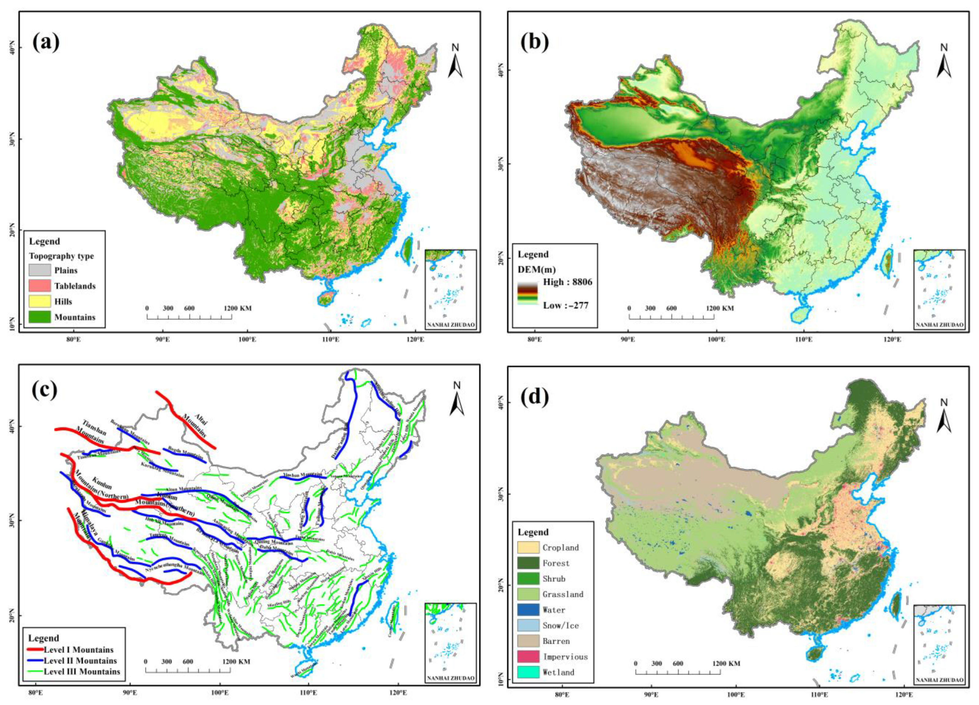
Figure 1. The spatial distribution of the Geomorphologic Atlas of the People’s Republic of China (1:1 million, (a)), digital Elevation Model data (b), major mountain ranges (c), land cover data (d).
Remotesensing 14 06309 g001
Figure 2. Technology roadmap.
Remotesensing 14 06309 g002
Figure 3. The spatial distribution of the average PM2.5 concentration during 2000–2019. This result is calculated by averaging all annual PM2.5 concentration data during 2000–2019 over China.
Remotesensing 14 06309 g003
Figure 4. Comparisons among the average PM2.5 concentrations during 2000–2019 for different topography types.
Remotesensing 14 06309 g004
Figure 5. The spatial distribution of the year frequency of annual PM2.5 concentration that exceeds 35 μg/m3 during 2000–2019 over China (a), the corresponding areal proportion under different levels of exceeding frequency (b), the area percentage of different topography types under different levels of exceeding frequency (ch). Note: Greater year frequency value means higher frequency.
Remotesensing 14 06309 g005
Figure 6. Superimposed distribution map of topography types and 35 μg/m3 dividing line (a), the length proportion of the 35 μg/m3 dividing line across the different topography types (b), the segmented length proportion across different elevation levels mountains in the mountains (c). Note: low elevation is altitude of less than 1000 m, middle elevation is altitude from 1000 to 3500 m, high elevation is altitude higher than 3500 m [60].
Remotesensing 14 06309 g006
Figure 7. The absolute PM2.5 concentration differences between the two sides of Level I–III mountains at different buffer zones. We first averaged the PM2.5 concentration pixels within the 15 km buffer zones of the two sides of the Level I mountains; then, the absolute value of the difference between the two average PM2.5 concentrations was calculated. The results for other buffer zones were found analogously.
Remotesensing 14 06309 g007
Figure 8. The changing curves between the mean and maximum PM2.5 concentrations and the DEM values (AV), and the corresponding trend detection in mean PM2.5 concentrations by M-K test (av) for the typic mountains. The mean PM2.5 concentrations (the orange lines) were the average PM2.5 concentrations based on pixels of each DEM value; analogously, the max PM2.5 concentrations (the blue lines) were the maximum PM2.5 concentrations based on pixels of each DEM value.
Remotesensing 14 06309 g008
Table 1. Classification system of the basic geomorphologic types of Chinese territory [60].
NO.Geomorphologic TypesRelief Amplitude
1Plains<30 m
2Platforms>30 m
3Hills<200 m
4Low-relief mountains200–500 m
5Middle-relief mountains500–1000 m
6High-relief mountains1000–2500 m
7Highest-relief mountains>2500 m
Table 2. The absolute PM2.5 concentration differences between the two sides of Level I–III mountains at different buffer zones. We first calculated the absolute PM2.5 concentration differences between the two sides of each mountain, and the absolute values of all the mountains at each level were then averaged and are provided in the table below. As there are many mountains, only the mountains with absolute PM2.5 concentration differences between their left and right sides greater than 10 μg/m3 were typically shown in the table below, and these mountains were taken as the typical mountains.
Level of MountainsMountains Name15 km30 km45 km60 km75 km90 km105 km
Level I MountainsAll Level I mountains0.593.175.577.328.3210.1611.76
Level I MountainsKunlun Mountains (Northern) 13.0917.6221.6525.2928.21
Level II MountainsAll Level II mountains2.233.574.215.025.856.617.22
Level II MountainsT’aihang Mountains 12.7616.7720.7823.4124.9326.24
Level II MountainsTianshan Mountains 11.7417.0819.4919.8921.41
Level II MountainsLuliang Mountains 16.2515.6713.8712.1911.2711.90
Level II MountainsQinling Mountains10.2513.8015.3516.1415.4915.0214.59
Level II MountainsBogda Mountains 10.3813.4015.20
Level II MountainsQilian Mountains 11.9413.9014.6614.81
Level II MountainsAltun Mountains 11.59
Level II MountainsQimantag Mountains 10.40
Level III MountainsAll Level III mountains3.423.874.14.354.474.485.18
Level III MountainsHora Mountains19.6224.5525.1729.0932.3031.7929.49
Level III MountainsTaiyue Mountains28.2329.5020.8310.48
Level III MountainsLongmen Mountains 13.9218.6321.3723.6824.73
Level III MountainsFangdou Mountains13.2816.7719.4320.3213.9914.5014.87
Level III MountainsDaqingshan Mountains 15.2017.4717.4915.6113.9012.92
Level III MountainsZhongtiao Mountains16.7110.15 14.7415.82
Level III MountainsYanshan Mountains 11.4014.58
Level III MountainsHengshan Mountains 14.0810.37
Level III MountainsDaliang Mountains 10.6913.6711.62
Level III MountainsMufu Mountains 10.6313.59
Level III MountainsWudang Mountains11.0212.44
Level III MountainsTolai Mountains 10.0711.5012.31
Level III MountainsQionglai Mountains 10.7012.25
Level III MountainsAyirariju Mountains 11.89
Level III MountainsDaxue Mountains 10.0611.64
Level III MountainsXionger Mountains 11.40
Level III MountainsHelan Mountains 11.40
Level III MountainsQianshan Mountains 10.7511.37
Table 3. The results of M-K test for the typical mountains.
Mountains’ LevelMountains’ NameUFk ValueThe Starting Position (m)
DEM (m)
Max PM2.5 Value ① (μg/m3)Max PM2.5 Value ② (μg/m3)Mean PM2.5 Value ① (μg/m3)Mean PM2.5 Value ② (μg/m3)Max PM2.5 Pollution Blocking Effects (μg/m3)
All typical mountains−99.41 **163228102.3198.3852.8359.7139.30%
Level IKunlun Mountains (North)−93.22 **1963832102.31102.3162.1962.4738.93%
Level IILüliang Mountains−72.07 **65039796.6496.6463.7165.1532.59%
Level IIQilian Mountains−85.56 **174564952.9252.9241.3337.3929.34%
Level IITaihang Mountains−68.07 **14320898.3898.3852.8375.3123.45%
Level IIQingling Mountains−84.93 **47515685.5585.5471.4667.4521.15%
Level IIAltuns Mountains−102.40 **8454269.0465.3556.6760.767.04%
Level IIIMufu Mountains−56.97 **33232971.8471.8361.5445.5936.54%
Level IIIDaqingshan Mountains−53.14 **10578152.4252.4230.7433.3136.46%
Level IIILongmen Mountains−93.62 **60424081.4881.4749.3253.3734.50%
Level IIIHelan Mountains−62.71 **118320359.6059.6041.6340.6131.86%
Level IIIFangdou Mountains−50.38 **1799266.4866.4854.3645.6931.28%
Level IIIYanshan Mountains−65.13 **5811065.2765.2739.6147.2227.65%
Level IIIHengshan Mountains−72.91 **31114972.4172.4056.0154.1825.17%
Level IIIHuala Mountains−78.32 **119132472.2672.2657.4658.5418.99%
Level IIIDa Xueshan Mountains−88.78 **6526460.3360.0657.6949.4117.73%
Level IIIQionglai Mountains−82.10 **5449585.8885.8875.0172.3015.81%
Level IIIWudang Mountains−75.54 **1314966.0962.1858.3058.456.00%
Level IIIXiong’er Mountains−42.36 **121080.3477.0676.7776.770.37%
Level IIITaiyue Mountains−66.65 **435087.7585.6885.5085.500.21%
Level IIIDaliang Mountains−98.49 **249075.8773.9473.9473.940.00%
Level IIIZhongtiao Mountains−68.27 **122081.2580.3180.3180.310.00%
The UFk value is a variable used to characterize the upward or downward trend of a series by M-K test, and an UFk value below 0 indicates a downtrend, whereas an UFk value above 0 indicates an upward trend. “**” representing a confidence level of p < 0.001. This is achieved based on the 105 km buffer zone for the purpose of covering the large mountains. The starting position is the elevation for the position at which blocking effects begin, as well as the position at which the positive UFk value shifts into negative one. △DEM is the difference of the elevation for the starting position and the lowest elevation in the 105 km buffer zone (i.e., the mountains’ foot). Max PM2.5 value ① is the max PM2.5 value within the 105 km buffer zone, which is the highest pixel value of the PM2.5 concentration within the considered regions of the mountains. Max PM2.5 value ② is the max PM2.5 value within the regions from the mountains’ foot to the starting position, which is the highest pixel value of the PM2.5 concentration within the considered regions of the mountains. Mean PM2.5 value ① is the mean PM2.5 value at the mountains’ foot, which is the averaged PM2.5 concentration for the pixels located at the mountains’ foot. The mountains’ foot is represented by the area with the lowest elevation within the 105 km buffer zone. Mean PM2.5 value ② is the mean PM2.5 value at the position at which blocking effects begin, which is the averaged PM2.5 concentration for the pixels located at the starting position. Max PM2.5 pollution blocking effects is the PM2.5 concentration declining amplitude calculated by the mean PM2.5 value at the starting position and the max PM2.5 value within regions from the mountains’ foot to the starting position.
Publisher’s Note: MDPI stays neutral with regard to jurisdictional claims in published maps and institutional affiliations.