Article

A Filtering Method for LiDAR Point Cloud Based on Multi-Scale CNN with Attention Mechanism

1
College of Oceanography and Space Informatics, China University of Petroleum (East China), Qingdao 266580, China
2
Laboratory for Marine Mineral Resources, Qingdao National Laboratory for Marine Science and Technology, Qingdao 266071, China
*
Author to whom correspondence should be addressed.
Remote Sens. 2022, 14(23), 6170; https://doi.org/10.3390/rs14236170
Submission received: 25 September 2022 / Revised: 2 December 2022 / Accepted: 2 December 2022 / Published: 6 December 2022

Abstract

:
Point cloud filtering is an important prerequisite for three-dimensional surface modeling with high precision based on LiDAR data. To cope with the issues of low filtering accuracy or excessive model complexity in traditional filtering algorithms, this paper proposes a filtering method for LiDAR point cloud based on a multi-scale convolutional neural network incorporated with the attention mechanism. Firstly, a regular image patch centering on each point is constructed based on the elevation information of point clouds. As thus, the point cloud filtering problem is transformed into the image classification problem. Then, considering the ability of multi-scale convolution to extract features at different scales and the potential of the attention mechanism to capture key information in images, a multi-scale convolutional neural network framework is constructed, and the attention mechanism is incorporated to coordinate multi-scale convolution kernel with channel and spatial attention modules. After this, the feature maps of the LiDAR point clouds can be acquired at different scales. For these feature maps, the weights of each channel layer and different spatial regions can be further tuned adaptively, which makes the network training more targeted, thereby improving the model performance for image classification and eventually separating of ground points and non-ground points preferably. Finally, the proposed method is compared with the cloth simulation filtering method (CSF), deep neural network method (DNN), k-nearest neighbor method (KNN), deep convolutional neural network method (DCNN) and scale-irrelevant and terrain-adaptive method (SITA) for the standard ISPRS dataset of point cloud filtering and the filter dataset of Qinghai. The experimental results show that the proposed method can obtain lower classification errors, which proves the superiority of this method in point cloud filtering.

Graphical Abstract

1. Introduction

Compared to traditional remote sensing techniques, the light detection and ranging (LiDAR) system can obtain high-precision three-dimensional information of ground objects rapidly and efficiently. Therefore, it is widely used in digital terrain model (DTM) generation [1,2,3,4,5], 3D modeling of buildings [6,7,8,9], hydrological modeling [10], forest inventory and management [11,12,13,14,15,16,17] and many other application fields. When acquiring data, the LiDAR system not only provides high-precision and high-density topographic surface information, but also records the information of non-topographic surface objects, such as buildings, trees, etc., [18]. As a result, in some measurement tasks closely related to the surface morphology, such as landslide detection [19], erosion and deposition quantification [20], channel bed morphology identification [21] and DTM extraction [22], it is necessary to separate the non-ground points from ground points in the point clouds, by means of the so-called point cloud filtering methods [23,24]. Previous studies have revealed that it is extremely challenging to perform point cloud filtering for particularly complex scenarios, such as urban areas and highly rugged surface environments [25]. This is mainly because complex topographic structures such as trees and buildings in urban areas often lead to misclassification of ground points [26]. In addition, in the forest measurement process, the filtering tasks may become more difficult due to the sparse ground points collected by LiDAR [27]. Over the past two decades, a series of filtering methods have been proposed to automatically classify ground points and non-ground points. Each method has its advantages and disadvantages, and the performance of these filtering methods varies from scene to scene. Traditional point cloud filtering algorithms are mostly based on unsupervised classification, which distinguishes ground points from non-ground points based on their different height, geometry or slope characteristics. These traditional algorithms have a preferable filtering effect in low-complexity scenarios such as flat terrain areas or buildings with simple structures. However, the results may be unsatisfactory in some high-complexity scenarios [28]. For example, Zhao et al. [29] have found that the detection results are sensitive to the selection of the optimal window size when detecting ground seed points using morphological open operation. The multi-resolution hierarchical classification (MHC) algorithm, proposed by Chen et al. [30], has superior performance in urban areas, but poor extraction effect for steep terrain.
To settle the issues of low filtering accuracy or excessive model complexity in traditional filtering algorithms, some researchers have proposed the use of machine learning methods to better solve the point cloud filtering problem. The filtering algorithms based on machine learning treat point cloud filtering as a binary classification problem, that is, all points are classified as ground points or non-ground points. Based on the features acquired from the point cloud data, the filtering tasks can thus be achieved by training some machine learning model, such as a conditional random field (CRF) [31], support vector machine (SVM) [32], random forest (RF) [33], etc. For example, the Bayesian network-based point clouds classification method proposed by Kang et al. [34] combines the geometric features of point clouds and the spectral features of images to classify the ground points, vegetation points and building points in the survey areas. Zhang et al. [35] designed a support vector machine to classify point clouds in urban areas. However, the filtering results of the above methods are not so satisfactory, because these methods are mostly based on local features, without considering the context relationship between taxonomic units. In addition, the training of machine learning models usually requires a large number of input features, which makes the task of feature extraction especially challenging.
In the past few decades, deep learning methods have been widely used in image classification [36]. As the typical representative, convolutional neural networks (CNNs) can directly obtain spatial context information from images, so as to extract complex features more effectively [37]. In recent years, CNNs have been successfully applied to point clouds processing, which can be mainly categorized as multi-view-based network models [38,39], voxel-based network models [40,41] and point-based network models [42,43]. Specifically, the multi-view-based methods convert point clouds into multi-view images and classify the converted images by using a neural network. However, the circumstance of point cloud occlusion is inevitable during the conversion process, thus leaving the classification results unsatisfactory. To solve this problem, the point clouds are converted into 3D voxels, whose features are extracted using CNNs in [40,41]. Although these methods can classify the point clouds, the introduced voxel structure also causes a lot of data redundancy. Later, the point-based network models are proposed by [42,43], with the ability of capturing the characteristics of the object surface from different angles and scales. These models have been successfully applied to the classification of indoor 3D points or building facades.
However, the methods mentioned above assign the same weights to the extracted features, which leads to the increase of unnecessary computation and fails to highlight the differences between the primary features and the secondary features, thus limiting the further improvement of classification performance. Fortunately, the attention mechanism can automatically focus on the target areas according to the salient features of the image. In the image classification tasks, the attention mechanism can adaptively assign different weights to each spectral channel and spatial region, so as to characterize their different contributions to the classification task, which eventually improve the classification performance of the network models. Therefore, the introduction of an attention mechanism is expected to provide a new way to solve the problem of point cloud filtering.
To further improve the accuracy of point cloud filtering, a new point cloud filtering method is proposed by introducing the channel and spatial attention modules [44]. The method mainly includes two processing stages, that is, the conversion of the point clouds to images and the construction and training of the network model. In particular, to avoid serious information loss, this paper does not convert point cloud data to multi-view images, but constructs regular three-channel images centering around each point based on the elevation coordinates of point clouds [45], thereby turning the point cloud filtering problem into an image classification task. In addition, in the model construction and training stage, the introduced channel and spatial attention modules can assign adaptive weights for each spectral channel and different spatial regions of the LiDAR point cloud feature maps, which allows the model to be trained more efficiently, obtains better image classification results and, finally, achieves high-precision point cloud filtering.

2. Method

To better solve the problem of point cloud filtering in complex terrain areas, this paper proposes a filtering method for LiDAR point cloud based on a multi-scale CNN with an attention mechanism. The method consists of two stages: (1) establishing a mapping relationship from point clouds to RGB images; (2) building a multi-scale CNN model with an attention mechanism to achieve images classification. During the first stage, a two-dimensional “square window” is defined with fixed size. By sliding such window, centering on each point, the whole point cloud is then traversed and converted into RGB images. These transformed image data are divided into a training set, verification set and test set to facilitate subsequent experiments. During the second stage, an image classification model is built based on a multi-scale convolutional neural network with attention mechanism (MSCNN-AM). In this model, the attention mechanism is introduced into the multi-scale convolution to capture the spatial significance differences from the features of different scales, so as to improve the classification accuracy. Finally, the trained model is applied to the test set, with the LiDAR point cloud filtering results output. The overall flow of the proposed method is shown in Figure 1.

2.1. Point to Image Conversion

Different from regular image data, LiDAR point cloud data represent discrete points with disordered distribution in space. Considering that these discrete points cannot be directly processed by CNNs, it is necessary to convert LiDAR point cloud data into regular image data. Firstly, to improve the convergence speed of the model and reduce the computational cost, the X-axis and Y-axis coordinate values of the LiDAR point cloud are standardized as follows:
{ x = x μ σ y = y μ σ
where x and y denote the initial coordinate values of each sample on the X and Y axes, μ and σ are the mean value and the standard deviation of all sample data, x and y are the standardized coordinate value of each sample on the X-axis and Y-axis.
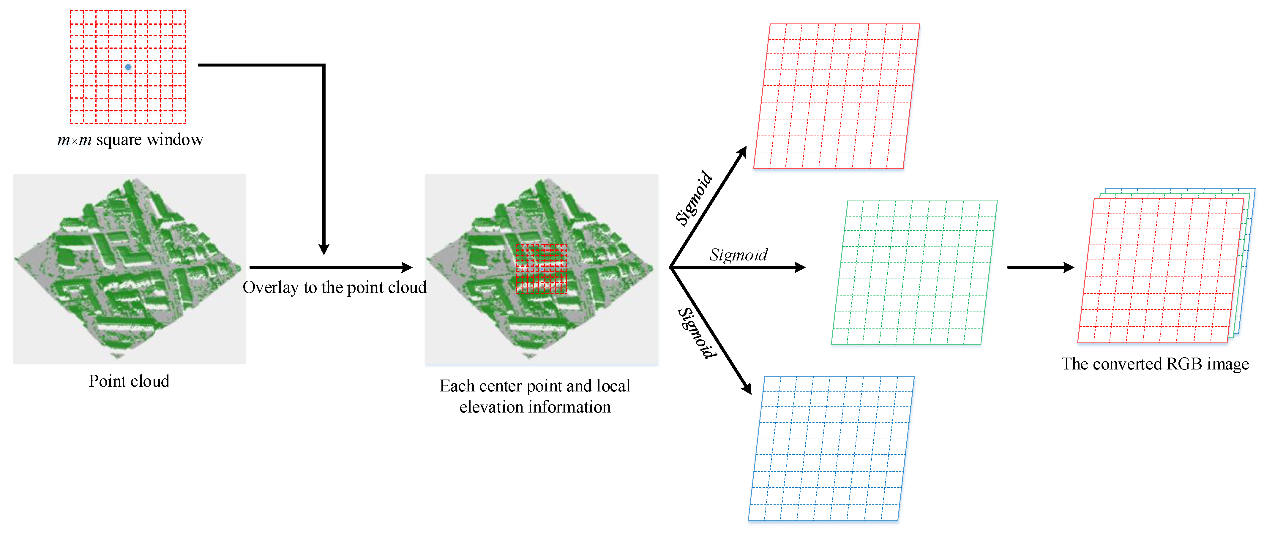
Secondly, a two-dimensional “square window” is defined and divided into m × m grids of the same size. By moving the “square window” so that a certain point p i to be classified becomes the center of the “square window”, all neighboring points within the window around the current point p i will be divided into these m × m different grids. Then, each grid of the “square window” can be converted into an RGB vector based on the elevation difference between the points within the grid and the central point p i . Specifically, the maximum elevation Z m a x , minimum elevation Z m i n and average elevation Z m e a n for all points within each grid are obtained, and then the elevation differences between Z m a x , Z m i n , Z m e a n and the elevation Z i of the current point p i are respectively calculated. By introducing some kind of activation function, the calculated elevation differences are then converted into red, green and blue pixel values according to Equation (2).
{ F r e d = 255 × S i g m o i d ( Z m a x Z i ) 0.5 F g r e e n = 255 × S i g m o i d ( Z m i n Z i ) 0.5 F b l u e = 255 × S i g m o i d ( Z m e a n Z i ) 0.5
where Z i is the elevation value of the current point p i , the symbol represents the operation of rounding down, and the Sigmoid function is expressed as follows.
S i g m o i d ( x ) = 1 ( 1 + e x )
Consequently, the whole “square window” is converted into a color image of size m × m × 3, as illustrated in Figure 2. By further taking each point to be classified as the center of the “square window” and adopting a similar approach as above mentioned, the whole point cloud is eventually traversed and converted into RGB images.

2.2. Attention Modules

There are usually obvious differences for the local features of point clouds located in different spatial regions. By effectively capturing these local features, it is expected to further improve the accuracy of image classification. As a means of focusing on local feature information, the attention mechanism is essentially to locate information in the region of interest while suppressing information in the irrelevant background region. As thus, the attention mechanism is introduced here for capturing the key information of point clouds, which is helpful to further improve the filtering effect of point clouds.

2.2.1. Channel Attention Module

In the CNNs, each channel of the feature maps actually plays a different role in information transmission. If each channel is regarded as equally important when performing feature extraction, the advantage of CNNs will not be fully played.
To this end, in the process of constructing a CNN, the channel attention module [44] is introduced for querying each channel of the feature maps, so as to determine which channels have a significant impact upon the classification results. After that, different weights are assigned to the channels according to their influence degree to reflect the difference in the contribution of different channels to the classification task. The detailed implementation process is shown in Figure 3 below.
The specific calculation procedure can be described as follows: Firstly, the spatial dimension of the input feature map F R C × H × W is “aggregated” by using the operations of global maximum pooling [46] and global average pooling [47], respectively, to generate two feature maps containing different spatial context information. Each feature map is a vector of C × 1 × 1 , represented by F m a x C and F a v g C , respectively. Then, the two feature maps are input into a two-layer shared fully connected neural network for further processing. This shared fully connected neural network consists of a multi-layer perceptron (MLP) and a hidden layer. To reduce parameter overhead, the number of neurons in the first layer is set to C / r , where the reduction rate r is set to 2, and the number of neurons in the second layer is C . After that, the two feature maps processed by the shared fully connected neural network are added together, and then activated by a Sigmoid function to generate the channel attention map M C R C × 1 × 1 , which is namely the weight corresponding to each channel. Finally, the attention map M C is weighted to the input feature map F by channel to produce the output feature map F . In short, the process flow of the channel attention module can be expressed mathematically as follows.
M C ( F ) = σ ( M L P ( M a x P o o l ( F ) ) + M L P ( A v g P o o l ( F ) ) )                           = σ ( W 1 ( W 0 ( F max C ) ) + W 1 ( W 0 ( F a v g C ) ) )
where σ denotes the Sigmoid function, and the weights W 0 R C / r × C and W 1 R C × C / r are shared for the input features of the fully connected neural network.
The channel attention module generates the weights corresponding to different channels, which makes the ultimate classification network model focus on the training process of each channel based on these different attention weights, thereby improving its classification performance.

2.2.2. Spatial Attention Module

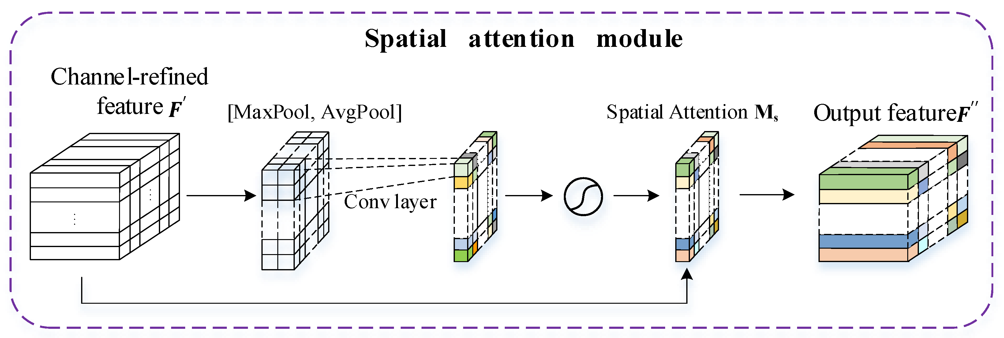
Different spatial regions in the image also have different degrees of contribution to the classification task, to which the regions related need to be paid close attention. By introducing a spatial attention module [44], these regions can be assigned different weights to further produce new features with spatial significance differences. The spatial attention module tends to indicate “where” in the input feature map is the salient information part, which is complementary to the channel attention module. The detailed implementation process is shown in Figure 4 below.
The specific calculation procedure can be described as follows: To enhance the salient contrast of different regions in the feature map, the operations of the maximum pooling and the average pooling are performed upon all pixels within the input feature map F along the channel dimension, yielding the maximum pooling feature map F m a x S R 1 × H × W and the average pooling feature map F a v g S R 1 × H × W . After that, the two feature maps are concatenated, producing a more informative two-channel feature map F m a x _ a v g S R 2 × H × W . By adopting a 3 × 3 convolution kernel processing upon the feature map F m a x _ a v g S , a new single-channel feature map can thus be obtained. If it is further activated by the Sigmoid function, the spatial attention map M S ( F )   R 1 × H × W is generated, with each pixel being assigned a weight. Finally, the spatial attention map M S and the input feature map F are multiplied pixel-by-pixel to yield F , which is the output feature processed by the spatial attention module. In short, the processing procedure of the above-mentioned spatial attention module can be expressed mathematically as follows.
M S ( F ) = σ ( f 7 × 7 ( [ M a x P o o l ( F ) ; A v g P o o l ( F ) ] ) )                             = σ ( f 7 × 7 ( [ F max S ; F a v g S ] ) )
where σ is the Sigmoid function, and f   7 × 7 denotes the convolution operation with a kernel size of 7 × 7.
The attention mechanism introduced in this paper consists of the channel attention module and the spatial attention module as mentioned above. Taking the given feature map F R C × H × W as input, the attention modules operate by sequentially building a 1D channel attention map M C R C × 1 × 1 and a 2D spatial attention map M S R 1 × H × W . The operation process of the overall attention modules can be summarized as follows.
F = M C ( F ) F F = M S ( F ) F
where the symbol ⨂ denotes the multiplication of elements. The attention values are propagated accordingly in such a manner: the channel attention propagates along the spatial dimension, while the spatial attention propagates along the channel dimension.

2.3. MSCNN-AM Model

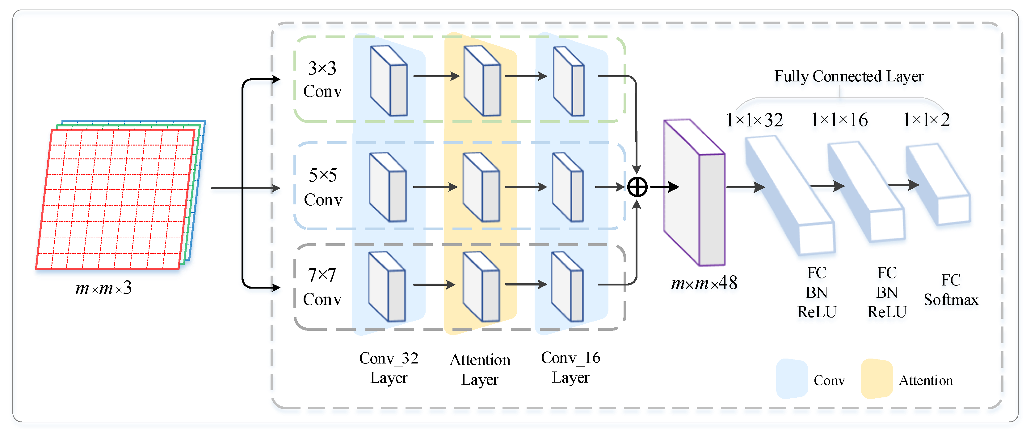
The MSCNN-AM model is mainly composed of five modules: the input layer, convolution layer (Conv), attention layer, fully connected layer and output layer, as shown in Figure 5. The input layer accepts the point-cloud-converted image f produced in Section 2.1. As the core block of the model, the convolution layer first adopts three convolution kernels of different scale to extract the features of the input image f via three branches, to generate different feature maps. What follows is weighting these feature maps respectively by the attention modules. After that, the second layer of multi-scale convolution is employed upon these weighted feature maps to acquire the ultimate feature maps. Finally, these feature maps via three branches are concatenated and input to the fully connected layer to complete the category judgment.
The specific implementation process of this model can be described as follows:
Firstly, the convolution kernels with sizes of 3 × 3, 5 × 5 and 7 × 7 are introduced to capture the local features of different scales from the images. Since CNNs usually have a large number of parameters, a batch normalization layer (BN) and a rectified linear unit layer (ReLU) are added to the convolution layer to prevent overfitting. Here, BN is used to normalize the data in each mini-batch according to the Formula (7) below.
y = x μ σ 2 + ε γ + β
During the training process, μ and σ 2 are the mean and variance of the input mini-batch data, respectively. The learning parameters γ and β represent the scaling factor and the shifting normalization value, and ε is a constant added to the mini-batch variance to maintain the numerical stability. The batch normalization can significantly accelerate the training of neural networks by reducing the overfitting and improving the learning rate. Therefore, the convolutional layer can be regarded as a joint operation of Conv-BN-ReLU.
Based on the above multi-scale convolution kernels, the initial feature map F can be obtained from image f via each of the three branches. Then, the above feature map F is transferred to the channel attention module and the spatial attention module as described in Section 2.2. The channel attention module outputs the feature map F by assigning the weights to each channel of feature map F on the basis of its significance. Then, the spatial attention module generates the feature map F by further assigning different weights to each pixel of the feature map F to highlight the spatial significance of different regions. Finally, by proceeding the second layer of multi-scale convolution upon feature map F , the feature map F can thus be obtained in each branch. It is worth noting that there are 32 convolution kernels in the first layer and 16 kernels in the second layer.
After the processing of above multi-scale convolutions and attention modules, the feature maps generated via the three branches have the same size of width, height and depth. Furthermore, by concatenating the feature maps via the three branches together along the channel dimension, the ultimate feature map with a size of m × m × 48 is obtained, which contains feature information of different scales.
For completing the category judgment, the ultimate feature map needs to be flattened to a one-dimensional vector and transferred into the fully connected layer module. The fully connected layer module consists of three layers, which are composed of 32, 16 and 2 neurons. In the fully connected layer module, each neuron of the current layer is connected to all neurons of the previous layer. As thus, the last layer outputs the category label of each image, which is tuned by the Softmax function. Then, the category label of the point cloud can be obtained according to the mapping relationship from the point cloud to the image. At this point, it is equivalent to having completed the filtering task of the point cloud.

3. Results

3.1. Datasets

3.1.1. ISPRS Filter Dataset

The first filter dataset used in this experiment is the standard point cloud dataset provided by the International Society for Photogrammetry and Remote Sensing (ISPRS) Working Group Ⅲ/3. The dataset includes a total of 15 samples, of which 9 samples are located in cities and 6 samples are located in rural areas. Among them, there are various complex terrain and ground objects, such as steep slopes, large buildings, low vegetation, etc., as shown in Table 1, which could be very helpful for better evaluating the proposed method in all aspects. In particular, the point spacing distances vary from 1 m to 1.5 m for the samples of Samp11-Samp42, and from 2 m to 3.5 m for the samples of Samp51-Samp71. All sample points are manually labeled as ground or non-ground. In addition, according to the geomorphological characteristics, all 15 samples are divided into 3 groups, which are the flat land, the gentle slope and the steep slope, as shown in Table 2.
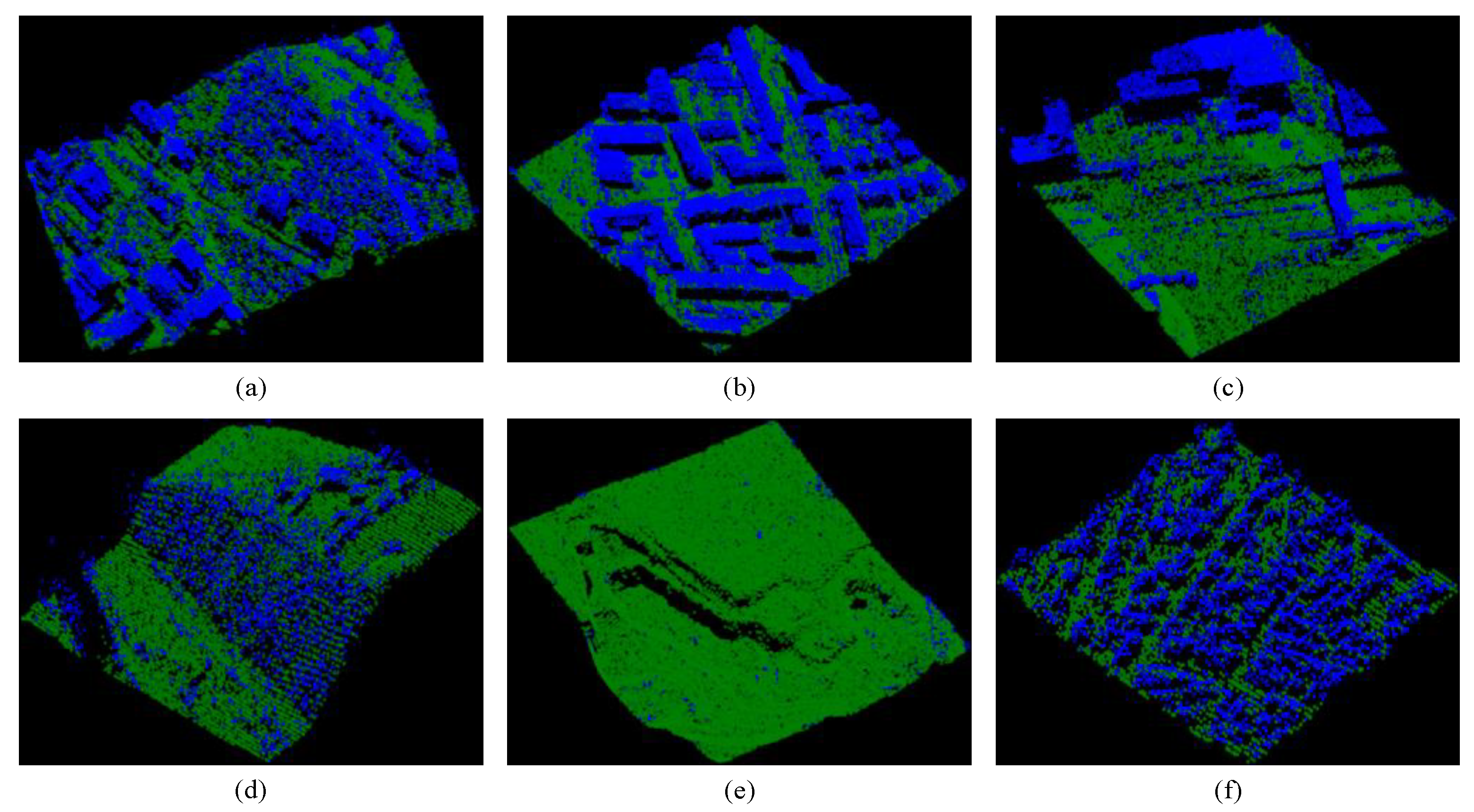
For an intuitive visualization of the point clouds, Figure 6 displays several labeled samples, which are randomly selected from the dataset. The green dot represents the real ground point, and the blue dot indicates part of the real non-ground object such as the building, the vehicle, the vegetation, etc.

3.1.2. The Filter Dataset of Qinghai

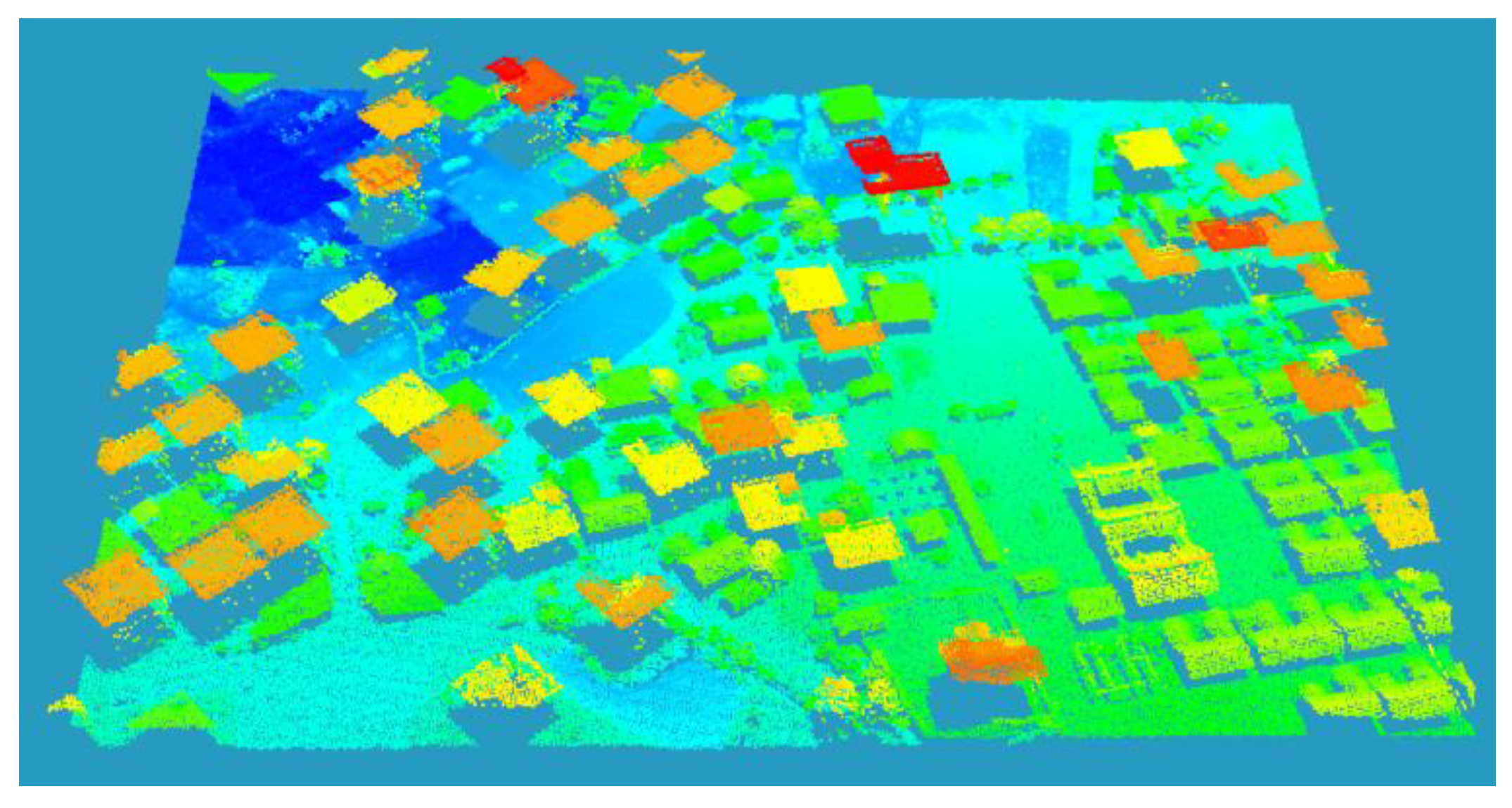
The filter dataset of Qinghai covers part of an urban area in Qinghai Province, with a length of about 297 m and a width of about 186 m, as shown in Figure 7. The terrain of this area is relatively flat and contains a large number of buildings and low vegetation, which is a typical urban area. The dataset has a high point density: about 4 to 5 points per square meter. In addition, there are 227,091 points in this dataset, all of which have been manually labeled as ground or non-ground (156,071 ground points and 71,020 non-ground points) for the convenience of subsequent experiments.
When conducting experiments on the above two datasets, 30% of the data from each dataset is taken as the training set, while 70% of the data is served as the test set to complete the model training and verify its performance. It should be noted that 10% of the training set is used as the validation set to check whether there will be overfitting during the model training stage.

3.2. Parameter Configuration

In the training process, an Adam optimizer is used to optimize the parameters of the model due to its advantages of accelerating the convergence speed and simplifying the parameter adjustment. The learning rate is initially set to be the same for each parameter, and adaptively evolves independently as the learning process progresses.
To better process the task of point cloud classification, the loss function of the MSCNN-AM model can be calculated as follows:
l o s s = 1 n [ i = 1 n j = 0 k 1 I { y ( i ) = j } log e w j T x ( i ) l k e w l T x ( i ) ]
where n is the batch size, which is prescribed to be 280. The category number, k, is set at 2 in the experiment. w is the weighting parameter; x denotes the output of the upper layer of the model; y ( i ) represents the category label of the ith sample. In addition, the indication function of I { y ( i ) = j } takes the value of 1 when y ( i ) = j , or 0 otherwise. The training process will be terminated when the accuracy meets the threshold requirements or reaches the maximum iterations (set to 256).

3.3. Accuracy Evaluation Indexes

In this paper, three indexes of type I error, type II error and total error are respectively employed to evaluate the classification accuracy of point cloud for the several filtering methods. As shown in Table 3, the type I error represents the percentage of ground points that are misclassified as non-ground points to the total number of ground points, while the type II error is the percentage of the number of non-ground points that are misclassified as ground points to the total number of non-ground points. As well the total error represents the percentage of the number of misclassified points to the total number of point clouds. It should be pointed out that the type I error usually has a greater impact on the results of the point cloud filtering compared with the type II error. This is because a larger type I error indicates that the filtered ground points are missing more severely, thus the later-constructed digital products such as DEM/DTM will have lower accuracy. Normally, a better filtering method obtains smaller type I error. For type II error, the secondary filtering strategy can be adopted to reduce its impact.

3.4. Result Analysis

To verify the effectiveness of the proposed method, the filtering performance of the proposed method is compared with that of the cloth simulation filtering method (CSF) [48], the deep neural network (DNN) filtering method [49], the K-nearest neighbor (KNN) filtering method [50], the deep convolutional neural network (DCNN) filtering method [45] and the scale-irrelevant and terrain-adaptive method (SITA) [51] upon the two datasets. Specifically, there are 4 hidden layers in the DNN model, and the neuron number is set to 16, 32, 32 and 16, respectively, for each hidden layer. These hidden layers are composed of fully connected layer (FC), batch normalization layer (BN) and rectified linear unit layer (ReLU). As is known to all, the K value significantly impacts the performance of the KNN filtering algorithm. After several experiments, it is found that the optimal separation effect can be achieved between ground points and non-ground points by setting K to 12. In the DCNN method, six layers with different number of convolution kernels are adopted to extract the single-scale features from the point-cloud-converted image, so as to complete the task of image classification and eventually achieve point cloud filtering. During the conversion stage from point cloud to image of the proposed MSCNN-AM method, the “square window” is divided into 9 × 9 grids, with each grid representing an actual size of 0.1 m × 0.1 m.

3.4.1. Result on ISPRS Dataset

In this paper, the filtering results of the proposed method are compared with those of the other five methods, as shown in Table 4. Obviously, the proposed MSCNN-AM method performs best in terms of the average type I error, type II error and total error upon the 15 samples. Compared with the CSF, KNN, DNN and SITA methods, the total error of the proposed method is reduced by 13.12%, 2.60%, 1.35% and 0.67%, respectively; the type I error is reduced by 18.01%, 0.19%, 0.17% and 0.67%; and the type II error is reduced by 0.36%, 13.99%, 9.07% and 0.07%. Such a satisfactory filtering effect can be mainly attributable to the powerful feature extraction capability of the deep learning network. In other words, when the samples are provided sufficiently, the classification performance of the trained model can be highly improved, thereby eventually separating ground points and non-ground points preferably. Compared with DCNN, the total error of the proposed method is reduced by 0.35%; the type I error is reduced by 0.37%; the type II error is reduced by 1.2%. The possible reasons can be summarized as the MSCNN-AM method not only employs the multi-scale convolution kernels to extract features of different scales, but also adaptively determines the contribution of each spectral channel and spatial region by introducing the attention mechanism, which makes the network training more targeted with the features of different importance. To clearly compare the classification error results, Figure 8 specifically displays the error line charts for the filtering methods of CSF, KNN, DNN, DCNN, SITA and MSCNN-AM upon 15 samples.
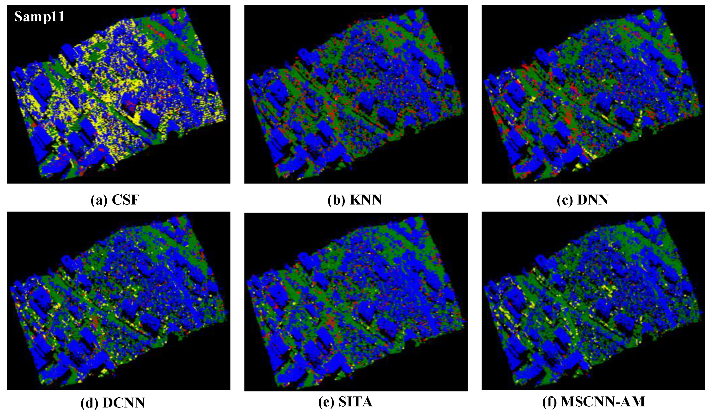
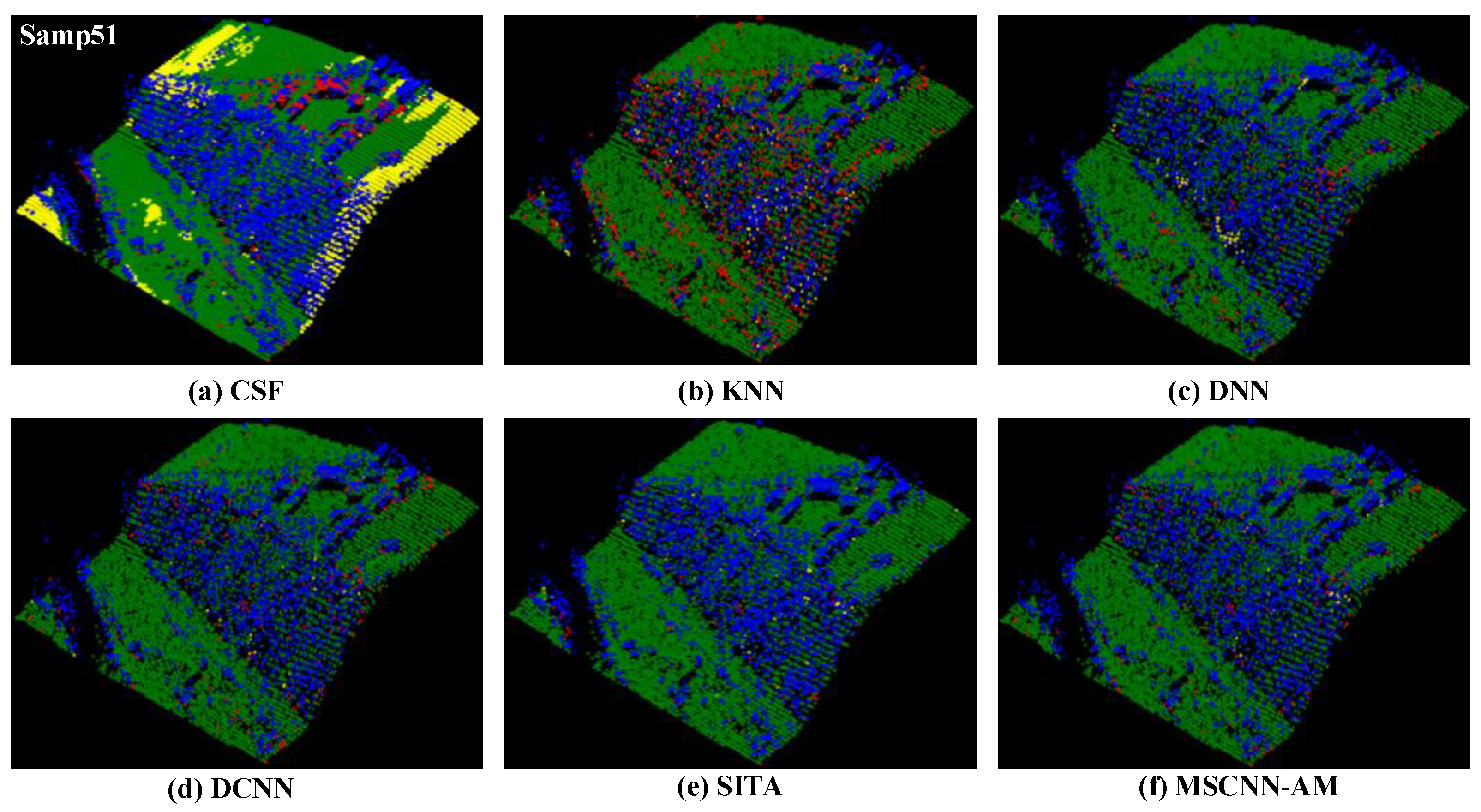
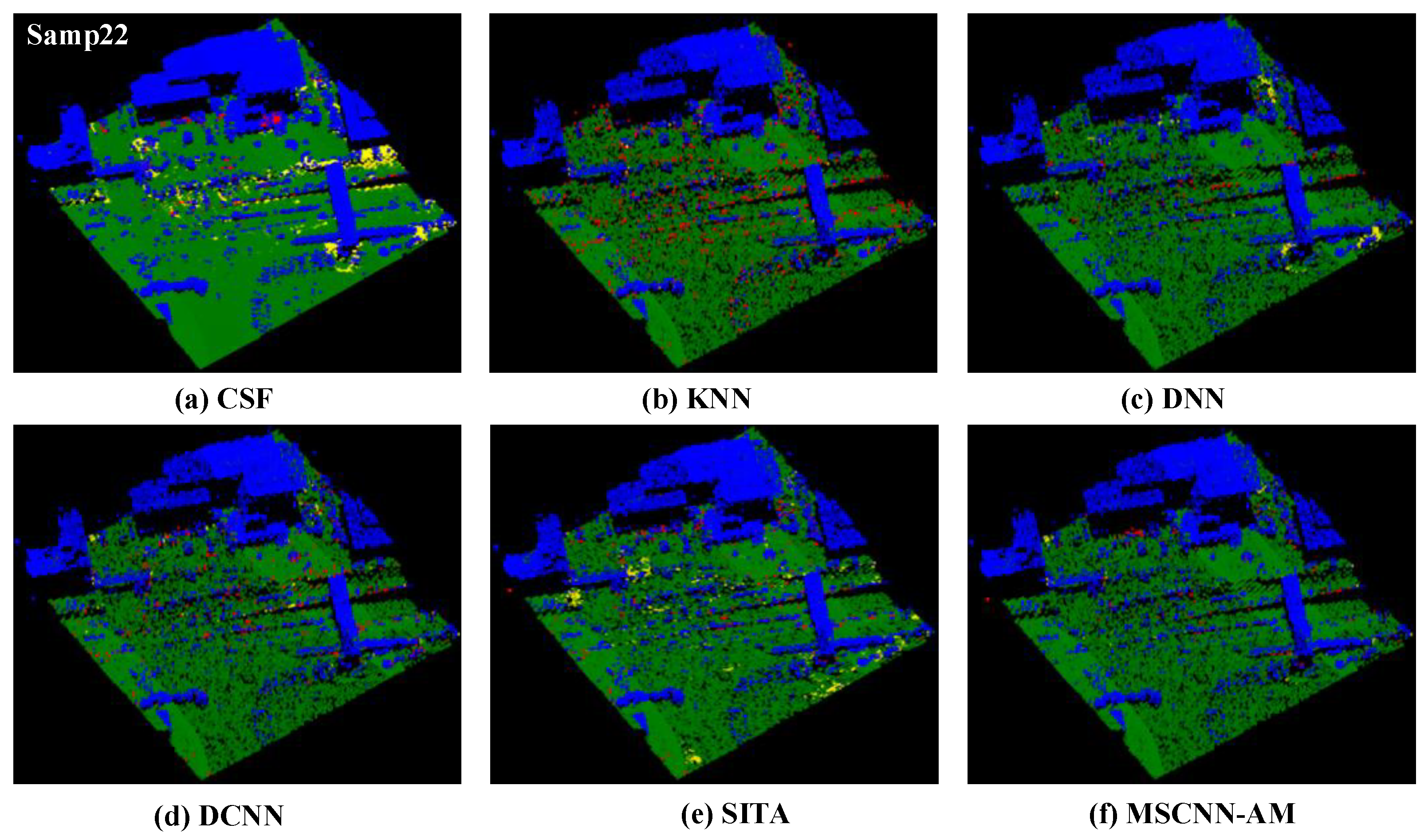
To further manifest the advantages of the proposed method, the comparative experiments of point cloud filtering are conducted on three different terrain samples with steep slope (Samp11 and Samp51), gentle slope (Samp22) and flat (Samp54) area.
In the steep slope area of Samp11, there are a lot of vegetation and buildings, which will cause the elevations of some ground points to be larger than the elevations of the adjacent non-ground points, thus increasing difficulties of the classification task. As shown in the experimental results of KNN, DNN and SITA, non-ground points in many areas are misclassified as ground points, which expands the type II error. These misclassified points are represented by red points in Figure 9b,c,e. Remarkably, this is rarely the case in the proposed method. Because the elevation information and local feature information of the point cloud are retained to the maximum extent when converting point cloud to image, the ground points and non-ground points can be better distinguished. As can be seen from Figure 9a, there are a lot of type I errors in the CSF method, which can be attributed to the insufficient feature extraction capacity of the traditional methods. Compared with the proposed method, although there are more type I errors in the results of DCNN on Samp11, its filtering results are significantly better than those of the KNN and DNN methods, which also demonstrates that the filtering method based on deep learning has certain advantages over machine learning methods to some extent. It should be noted that a small number of ground points are also misclassified into non-ground points within the vegetation and building areas in the proposed method, as indicated by the yellow points in Figure 9f. The main reason accounting for this situation is that in the slope area, the elevations of some ground points in the upper part of the slope are higher than the elevations of vegetation and buildings in the lower part of the slope, which increases the difficulty of distinguishing ground points from non-ground points. This is also a major challenge for point cloud filtering on such terrain containing complex features.
Different from Samp11, there is another sample of the steep terrain, Samp51, which has only vegetation but no buildings. In the results processed by the CSF method, a large number of ground points at the edge of the sample are misclassified as non-ground points, as shown by the yellow points in Figure 10a, and the overall classification effect is not satisfactory. In the steep slope area, a large number of non-ground points are misclassified into ground points in the experimental results of the KNN method, as indicated with the red points in Figure 10b. This can be attributed to the assumption that ground points are lower than the surrounding non-ground points in KNN. Whereas the other four methods all have satisfactory filtering results upon Samp51, and the proposed method performs best.
Samp22 is a gently sloping terrain, which contains buildings such as bridges and flight ladders and a small amount of low vegetation. In this sample, the classification effect of the bridge, especially its connection area with the ground, can be served as an important basis for evaluating the performance of the filtering methods. In the CSF, some ground points are still misclassified as non-ground points, leading to the large type I error. What is more, it can be seen from Figure 11b,d that in KNN and DCNN there are a few cases where non-ground points around the bridge are misclassified as ground points. This can be attributed to the existence of low vegetation around the bridge, whose elevation is smaller than that of the bridge. Although there are some ground points misclassified as non-ground points in DNN and SITA, their overall classification effect is better than that of KNN. In particular, the overall classification performance of the proposed method is the best, as only a small number of non-ground points are misclassified as ground points.
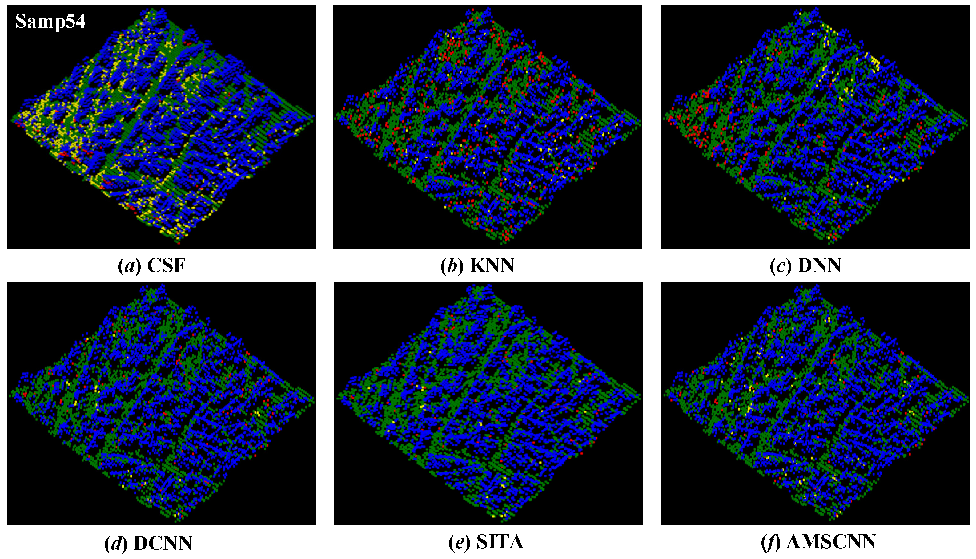
Samp54 is a flat area containing a large number of low-resolution buildings. Due to the low density of point cloud in the sample, the building contour is not clear enough, which leads to the situation where many non-ground points are misclassified into ground points in both KNN and DNN methods, as shown in red points in Figure 12b,c, respectively. In addition, low-resolution buildings still cause some ground points to be misclassified as non-ground points in CSF. By comparison, the methods of DCNN, SITA and MSCNN-AM perform better, which can be interpreted as these methods can better extract local features of buildings, so as to achieve satisfactory classification results even with low resolution.
In summary, the filtering experiments upon a variety of terrain data (steep slope, gentle slope and flat slope) have fully verified the applicability and robustness of the proposed method. Meanwhile, the proposed filtering method of MSCNN-AM exerts strong competitiveness compared to the two traditional filtering methods, with two filtering methods based on machine learning and one filtering method based on deep learning.

3.4.2. Result on Dataset of Qinghai

The proposed method and five other comparison methods are employed to the dataset of Qinghai for point cloud filtering, and Table 5 shows the comparative results of these methods. It can be seen that the proposed method performs optimally on this dataset. Considering that the Qinghai filtering data are collected from a relatively flat urban area, the structure is relatively simple, with only some buildings and low vegetation, so the task of separating ground points from non-ground points is relatively simple. Therefore, the filtering errors of several methods in Table 5 are not much different, but the proposed method still shows obvious advantages. This further verifies the generalization capacity of the proposed method.

4. Discussion

To verify the effectiveness of the multi-scale convolution and attention modules introduced in the proposed MSCNN-AM method, the ablation experiments on the ISPRS dataset are conducted by designing three different network architectures, which are the single scale convolutional neural network and the multi-scale convolutional neural networks integrated with and without the attention mechanism.
Throughout the whole experiment, all the conversion processes are kept consistent from point cloud to image. To be specific, the size of the convolution kernel is 7 × 7 in the single-scale neural network, and three different convolution kernel sizes of 7 × 7, 5 × 5 and 3 × 3 are employed for the multi-scale networks, as indicated in Figure 5. In addition, there are two designed convolutional layers in all the above neural networks. The convolution kernel number is 32 for the first layer, and 16 for the second layer.
As shown in Table 6, the results of ablation experiments indicate that the filtering accuracy based on the multi-scale convolutional neural network is higher than that using only a single-scale convolutional neural network. Moreover, compared with the multi-scale convolutional neural network without attention mechanism, the multi-scale convolutional neural network with attention mechanism has lower classification error and better filtering effect. On the whole, the ablation experiments fully confirm that the strategies of multi-scale convolution and attention mechanism adopted in this study have significantly positive effects on improving the filtering performance.
The proposed method in this paper uses 3 × 3, 5 × 5 and 7 × 7 convolution kernels for feature extraction in the model construction stage. To verify the superiority of these convolution kernel combinations, this paper further compares the effects of the other three convolution kernel combinations of different sizes for point cloud filtering, as shown in Table 7. It can be seen from the comparison results that the minimum total error and type I error can be obtained by using the convolution kernel combination with the size of 3 × 3, 5 × 5 and 7 × 7, and the overall effect is the best. Moreover, using the convolution kernel combination with a relatively small scale can reduce the time used for feature extraction and speed up the calculation.
In addition, to further verify whether the attention mechanism added in the model will increase the computational complexity and take more time, this paper performs the experiments using a computer equipped with AMD Ryzen5 5600H and NVIDIA GeForce RTX 3050 Laptop GPU. This experiment compares the time required for the model to process the ISPRS dataset with and without the attention mechanism, as shown in Table 8. As can be seen from the comparison results in the table, the training time with the attention mechanism model increased compared to the training time without the attention mechanism model, but the growth rate was not obvious, about 17%.

5. Conclusions

In this paper, a filtering method for LiDAR point cloud based on multi-scale CNN with attention mechanism is proposed to settle the problem of point cloud filtering in complex terrain. Firstly, the point cloud filtering problem is transformed into the image classification problem by centering on each point with a regular image patch, constructed relying on the elevation information of point clouds. The core idea of the proposed model is to combine the multi-scale convolution with the attention mechanism. In particular, the multi-scale convolution operation is employed to extract the features of different scales from the LiDAR point cloud, and the channel and spatial attention modules are introduced to adaptively correct the weights for each channel layer and different spatial regions of the feature maps. The practice of combining these two strategies can make the network training more targeted, thereby improving the model performance for image classification and eventually separating ground points and non-ground points preferably. Moreover, the proposed MSCNN-AM method has exerted strong competitiveness compared with five methods of CSF, KNN, DNN, DCNN and SITA on both the ISPRS filter dataset and the filter dataset of Qinghai. In addition, its advantages look even more pronounced when there are a large number of complex land cover types within the steep slope area. Considering that data conversion may cause the loss of partial information, it is necessary to explore a more effective high-fidelity conversion method from point cloud to image in future work.

Author Contributions

Conceptualization, B.W., H.W. and D.S.; methodology, B.W., H.W. and D.S.; software, H.W.; validation, B.W. and H.W.; formal analysis, B.W., H.W. and D.S.; data curation, B.W. and H.W.; writing-original draft preparation, B.W., H.W. and D.S.; writing-review and editing, B.W., H.W. and D.S.; project administration and funding acquisition, B.W. and D.S. All authors have read and agreed to the published version of the manuscript.

Funding

This work was supported by the Natural Science Foundation of Shandong Province under Grant ZR2022MD015, the Key Program of Joint Fund of the National Natural Science Foundation of China and Shandong Province under Grant U22A20586, the National Key Research and Development Program of China under Grant 2019YFC1509202, the National Natural Science Foundation of China under Grant 41701513, 41772350 and 61371189, and the Key Research and Development Program of Shandong Province under Grant 2019GGX101033.

Data Availability Statement

All the data given in this paper is available at corresponding web-sites.

Acknowledgments

We gratefully appreciate the editor and anonymous reviewers for their efforts and constructive comments, which have greatly improved the technical quality and presentation of this study.

Conflicts of Interest

The authors declare no conflict of interest.

Abbreviations

The following abbreviations are used in this manuscript:
BNbatch normalization
CNNconvolutional neural network
CRFconditional random Field
CSFcloth simulation filtering
DCNNdeep convolutional neural network
DEMdigital elevation model
DNNdeep neural network
DTMdigital terrain model
FCfully connected
ISPRSInternational Society for Photogrammetry and Remote Sensing
KNNk-nearest neighbor
LiDARlight detection and ranging
MHCmulti-resolution hierarchical classification
MLPmulti-layer perceptron
MSCNN-AMmulti-scale convolutional neural network with attention mechanism
ReLUrectified linear unit
RFrandom forest
SITAscale-irrelevant and terrain-adaptive
SVMsupport vector machine

References

  1. Meng, X.; Currit, N.; Zhao, K. Ground filtering algorithms for airborne LiDAR data: A review of critical issues. Remote Sens. 2010, 2, 833–860. [Google Scholar] [CrossRef] [Green Version]
  2. Sithole, G.; Vosselman, G. Experimental comparison of filter algorithms for bare-Earth extraction from airborne laser scanning point clouds. ISPRS J. Photogramm. Remote Sens. 2004, 59, 85–101. [Google Scholar] [CrossRef]
  3. Chen, Z.; Gao, B.; Devereux, B. State-of-the-art: DTM generation using airborne LIDAR data. Sensors 2017, 17, 150. [Google Scholar] [CrossRef] [PubMed] [Green Version]
  4. Liu, X. Airborne LiDAR for DEM generation: Some critical issues. Prog. Phys. Geogr. 2008, 32, 31–49. [Google Scholar]
  5. Guo, Q.; Li, W.; Yu, H.; Alvarez, O. Effects of topographic variability and lidar sampling density on several DEM interpolation methods. Photogramm. Eng. Remote Sens. 2010, 76, 701–712. [Google Scholar] [CrossRef] [Green Version]
  6. Rottensteiner, F.; Sohn, G.; Gerke, M.; Wegner, J.D.; Breitkopf, U.; Jung, J. Results of the ISPRS benchmark on urban object detection and 3D building reconstruction. ISPRS J. Photogramm. Remote Sens. 2014, 93, 256–271. [Google Scholar] [CrossRef]
  7. Wang, R. 3D building modeling using images and LiDAR: A review. Int. J. Image Data Fusion 2013, 4, 273–292. [Google Scholar] [CrossRef]
  8. Wang, R.; Peethambaran, J.; Chen, D. Lidar point clouds to 3-D urban models: A review. IEEE J. Sel. Top. Appl. Earth Obs. Remote Sens. 2018, 11, 606–627. [Google Scholar] [CrossRef]
  9. Sampath, A.; Shan, J. Segmentation and reconstruction of polyhedral building roofs from aerial lidar point clouds. IEEE Trans. Geosci. Remote Sens. 2009, 48, 1554–1567. [Google Scholar] [CrossRef]
  10. Bakuła, K. Multispectral airborne laser scanning-a new trend in the development of LiDAR technology. Arch. Fotogram. Kartogr. I Teledetekcji 2015, 27, 25–44. [Google Scholar]
  11. Hyyppä, J.; Hyyppä, H.; Leckie, D.; Gougeon, F.; Yu, X.; Maltamo, M. Review of methods of small-footprint airborne laser scanning for extracting forest inventory data in boreal forests. Int. J. Remote Sens. 2008, 29, 1339–1366. [Google Scholar] [CrossRef]
  12. Wang, Y.; Hyyppä, J.; Liang, X.; Kaartinen, H.; Yu, X.; Lindberg, E.; Holmgren, J.; Qin, Y.; Mallet, C.; Ferraz, A. International benchmarking of the individual tree detection methods for modeling 3-D canopy structure for silviculture and forest ecology using airborne laser scanning. IEEE Trans. Geosci. Remote Sens. 2016, 54, 5011–5027. [Google Scholar] [CrossRef]
  13. Hyyppä, J.; Yu, X.; Hyyppä, H.; Vastaranta, M.; Holopainen, M.; Kukko, A.; Kaartinen, H.; Jaakkola, A.; Vaaja, M.; Koskinen, J. Advances in forest inventory using airborne laser scanning. Remote Sens. 2012, 4, 1190–1207. [Google Scholar] [CrossRef] [Green Version]
  14. Wulder, M.A.; White, J.C.; Nelson, R.F.; Næsset, E.; Ørka, H.O.; Coops, N.C.; Hilker, T.; Bater, C.W.; Gobakken, T. Lidar sampling for large-area forest characterization: A review. Remote Sens. Environ. 2012, 121, 196–209. [Google Scholar] [CrossRef] [Green Version]
  15. Wallace, L.; Lucieer, A.; Watson, C.; Turner, D. Development of a UAV-LiDAR system with application to forest inventory. Remote Sens. 2012, 4, 1519–1543. [Google Scholar] [CrossRef] [Green Version]
  16. Drake, J.B.; Dubayah, R.O.; Clark, D.B.; Knox, R.G.; Blair, J.B.; Hofton, M.A.; Chazdon, R.L.; Weishampel, J.F.; Prince, S. Estimation of tropical forest structural characteristics using large-footprint lidar. Remote Sens. Environ. 2002, 79, 305–319. [Google Scholar] [CrossRef]
  17. Means, J.E.; Acker, S.A.; Fitt, B.J.; Renslow, M.; Emerson, L.; Hendrix, C.J. Predicting forest stand characteristics with airborne scanning lidar. Photogramm. Eng. Remote Sens. 2000, 66, 1367–1372. [Google Scholar]
  18. Wan, P.; Zhang, W.; Skidmore, A.K.; Qi, J.; Jin, X.; Yan, G.; Wang, T. A simple terrain relief index for tuning slope-related parameters of LiDAR ground filtering algorithms. ISPRS J. Photogramm. Remote Sens. 2018, 143, 181–190. [Google Scholar] [CrossRef]
  19. Chu, H.-J.; Wang, C.-K.; Huang, M.-L.; Lee, C.-C.; Liu, C.-Y.; Lin, C.-C. Effect of point density and interpolation of LiDAR-derived high-resolution DEMs on landscape scarp identification. GIScience Remote Sens. 2014, 51, 731–747. [Google Scholar] [CrossRef]
  20. Bremer, M.; Sass, O. Combining airborne and terrestrial laser scanning for quantifying erosion and deposition by a debris flow event. Geomorphology 2012, 138, 49–60. [Google Scholar] [CrossRef]
  21. Cavalli, M.; Tarolli, P.; Marchi, L.; Dalla Fontana, G. The effectiveness of airborne LiDAR data in the recognition of channel-bed morphology. Catena 2008, 73, 249–260. [Google Scholar] [CrossRef]
  22. Murphy, P.N.; Ogilvie, J.; Meng, F.R.; Arp, P. Stream network modelling using lidar and photogrammetric digital elevation models: A comparison and field verification. Hydrol. Processes Int. J. 2008, 22, 1747–1754. [Google Scholar] [CrossRef]
  23. Bayram, E.; Frossard, P.; Vural, E.; Alatan, A. Analysis of airborne LiDAR point clouds with spectral graph filtering. IEEE Geosci. Remote Sens. Lett. 2018, 15, 1284–1288. [Google Scholar] [CrossRef]
  24. Li, Y.; Yong, B.; Van Oosterom, P.; Lemmens, M.; Wu, H.; Ren, L.; Zheng, M.; Zhou, J. Airborne LiDAR data filtering based on geodesic transformations of mathematical morphology. Remote Sens. 2017, 9, 1104. [Google Scholar] [CrossRef] [Green Version]
  25. Nie, S.; Wang, C.; Dong, P.; Xi, X.; Luo, S.; Qin, H. A revised progressive TIN densification for filtering airborne LiDAR data. Measurement 2017, 104, 70–77. [Google Scholar] [CrossRef]
  26. Briese, C. Extraction of digital terrain models. In Airborne and Terrestrial Laser Scanning; Whittles Publishing: Dunbeath, UK, 2010; pp. 135–167. [Google Scholar]
  27. Zhang, J.; Hu, X.; Dai, H.; Qu, S. DEM extraction from ALS point clouds in forest areas via graph convolution network. Remote Sens. 2020, 12, 178. [Google Scholar] [CrossRef] [Green Version]
  28. Pfeifer, N.; Mandlburger, G. LiDAR data filtering and DTM generation. In Topographic Laser Ranging and Scanning; CRC Press: Boca Raton, FL, USA, 2017; pp. 307–334. [Google Scholar]
  29. Zhao, X.; Guo, Q.; Su, Y.; Xue, B. Improved progressive TIN densification filtering algorithm for airborne LiDAR data in forested areas. ISPRS J. Photogramm. Remote Sens. 2016, 117, 79–91. [Google Scholar] [CrossRef] [Green Version]
  30. Chen, C.; Li, Y.; Li, W.; Dai, H. A multiresolution hierarchical classification algorithm for filtering airborne LiDAR data. ISPRS J. Photogramm. Remote Sens. 2013, 82, 1–9. [Google Scholar] [CrossRef]
  31. Yang, F.; Davoine, F.; Wang, H.; Jin, Z. Continuous conditional random field convolution for point cloud segmentation. Pattern Recognit. 2022, 122, 108357. [Google Scholar] [CrossRef]
  32. Hsu, C.-W.; Lin, C.-J. A comparison of methods for multiclass support vector machines. IEEE Trans. Neural Netw. 2002, 13, 415–425. [Google Scholar]
  33. Breiman, L. Random forests. Mach. Learn. 2001, 45, 5–32. [Google Scholar] [CrossRef] [Green Version]
  34. Kang, Z.; Yang, J.; Zhong, R. A bayesian-network-based classification method integrating airborne lidar data with optical images. IEEE J. Sel. Top. Appl. Earth Obs. Remote Sens. 2016, 10, 1651–1661. [Google Scholar] [CrossRef]
  35. Zhang, J.; Lin, X.; Ning, X. SVM-based classification of segmented airborne LiDAR point clouds in urban areas. Remote Sens. 2013, 5, 3749–3775. [Google Scholar] [CrossRef] [Green Version]
  36. Chen, C.; Guo, J.; Wu, H.; Li, Y.; Shi, B. Performance Comparison of Filtering Algorithms for High-Density Airborne LiDAR Point Clouds over Complex LandScapes. Remote Sens. 2021, 13, 2663. [Google Scholar] [CrossRef]
  37. Rizaldy, A.; Persello, C.; Gevaert, C.; Oude Elberink, S.; Vosselman, G. Ground and multi-class classification of airborne laser scanner point clouds using fully convolutional networks. Remote Sens. 2018, 10, 1723. [Google Scholar] [CrossRef] [Green Version]
  38. Su, H.; Maji, S.; Kalogerakis, E.; Learned-Miller, E. Multi-view convolutional neural networks for 3D shape recognition. In Proceedings of the IEEE International Conference on Computer Vision, Washington, DC, USA, 20–23 June 1995; pp. 945–953. [Google Scholar]
  39. Qi, C.R.; Su, H.; Nießner, M.; Dai, A.; Yan, M.; Guibas, L.J. Volumetric and multi-view cnns for object classification on 3d data. In Proceedings of the IEEE Conference on Computer Vision and Pattern Recognition, New Orleans, LA, USA, 17–19 June 1997; pp. 5648–5656. [Google Scholar]
  40. Maturana, D.; Scherer, S. Voxnet: A 3D convolutional neural network for real-time object recognition. In Proceedings of the 2015 IEEE/RSJ International Conference on Intelligent Robots and Systems (IROS), Hamburg, Germany, 28 September–October 2 2015; pp. 922–928. [Google Scholar]
  41. Zhou, Y.; Tuzel, O. Voxelnet: End-to-end learning for point cloud based 3D object detection. In Proceedings of the IEEE Conference on Computer Vision and Pattern Recognition, Salt Lake City, UT, USA, 18–23 June 2018; pp. 4490–4499. [Google Scholar]
  42. Qi, C.R.; Su, H.; Mo, K.; Guibas, L.J. Pointnet: Deep learning on point sets for 3D classification and segmentation. In Proceedings of the IEEE Conference on Computer Vision and Pattern Recognition, Salt Lake City, UT, USA, 18–23 June 2018; pp. 652–660. [Google Scholar]
  43. Qi, C.R.; Yi, L.; Su, H.; Guibas, L.J. Pointnet++: Deep hierarchical feature learning on point sets in a metric space. In Proceedings of the 31st Conference on Neural Information Processing Systems (NIPS 2017), Long Beach, CA, USA, 4–9 December 2017; p. 30. [Google Scholar]
  44. Woo, S.; Park, J.; Lee, J.-Y.; Kweon, I.S. Cbam: Convolutional block attention module. In Proceedings of the European Conference on Computer Vision (ECCV), Munich, Germany, 8–14 September 2018; pp. 3–19. [Google Scholar]
  45. Hu, X.; Yuan, Y. Deep-learning-based classification for DTM extraction from ALS point cloud. Remote Sens. 2016, 8, 730. [Google Scholar] [CrossRef] [Green Version]
  46. Lin, M.; Chen, Q.; Yan, S. Network in network. arXiv 2013, arXiv:1312.4400. [Google Scholar]
  47. Hu, J.; Shen, L.; Sun, G. Squeeze-and-excitation networks. In Proceedings of the 2018 IEEE/CVF Conference on Computer Vision and Pattern Recognition, Salt Lake City, UT, USA, 18–23 June 2018; pp. 7132–7141. [Google Scholar]
  48. Zhang, W.; Qi, J.; Wan, P.; Wang, H.; Xie, D.; Wang, X.; Yan, G. An easy-to-use airborne LiDAR data filtering method based on cloth simulation. Remote Sens. 2016, 8, 501. [Google Scholar] [CrossRef]
  49. Martins, V.S.; Kaleita, A.L.; Gelder, B.K.; Nagel, G.W.; Maciel, D.A. Deep neural network for complex open-water wetland mapping using high-resolution WorldView-3 and airborne LiDAR data. Int. J. Appl. Earth Obs. Geoinf. 2020, 93, 102215. [Google Scholar] [CrossRef]
  50. Chen, B.; Shi, S.; Gong, W.; Zhang, Q.; Yang, J.; Du, L.; Sun, J.; Zhang, Z.; Song, S. Multispectral LiDAR point cloud classification: A two-step approach. Remote Sens. 2017, 9, 373. [Google Scholar] [CrossRef] [Green Version]
  51. Chen, C.; Chang, B.; Li, Y.; Shi, B. Filtering airborne LiDAR point clouds based on a scale-irrelevant and terrain-adaptive approach. Measurement 2021, 171, 108756. [Google Scholar] [CrossRef]
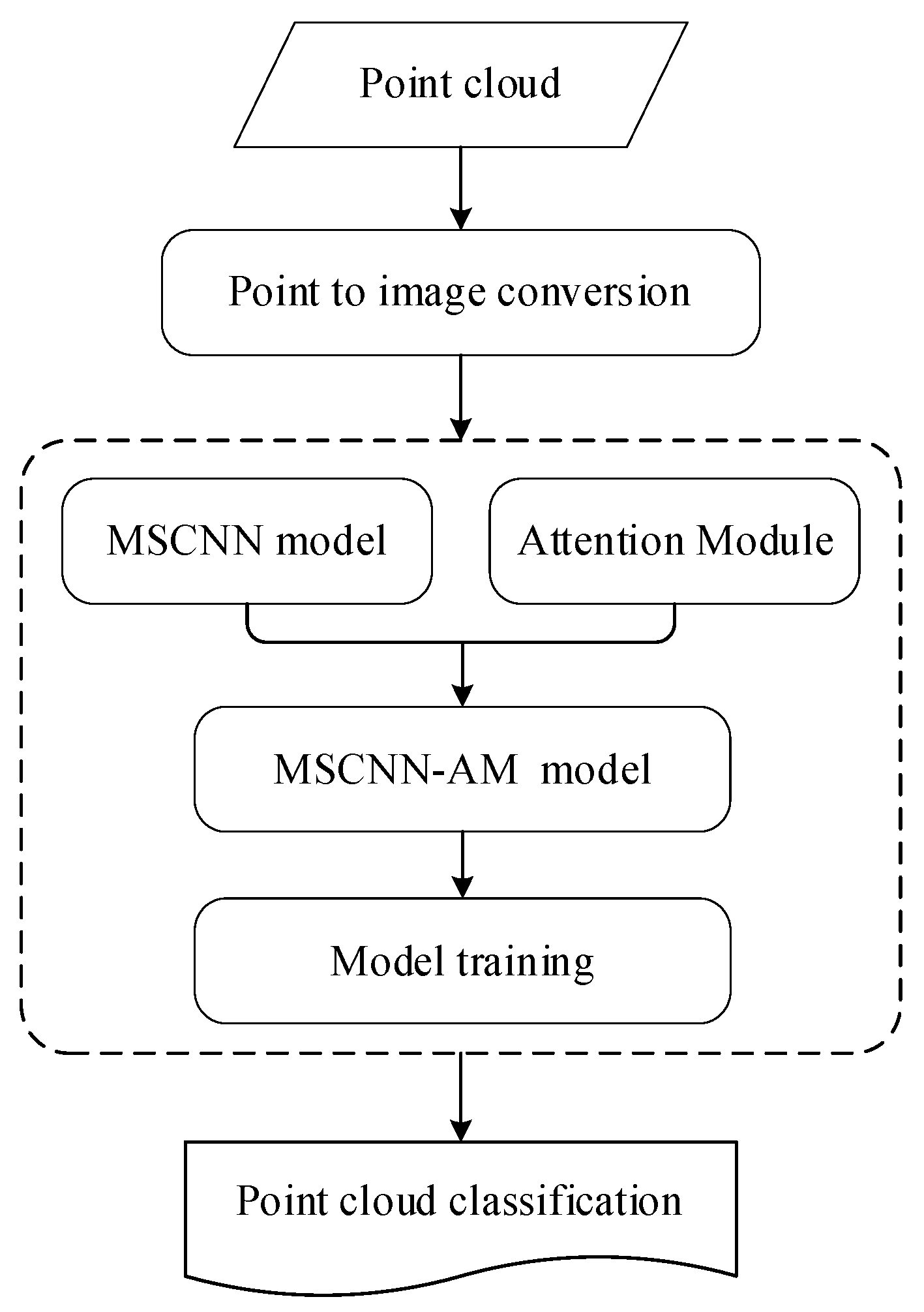
Figure 1. The overall workflow of the proposed point cloud filtering method.
Remotesensing 14 06170 g001
Figure 2. Schematic diagram of converting LiDAR point cloud to RGB image.
Remotesensing 14 06170 g002
Figure 3. Schematic diagram of the channel attention module.
Remotesensing 14 06170 g003
Figure 4. Schematic diagram of the spatial attention module.
Remotesensing 14 06170 g004
Figure 5. The proposed network framework of MSCNN-AM for point clouds filtering.
Remotesensing 14 06170 g005
Figure 6. Several samples of the ISPRS dataset. (a) Samp11; (b) Samp12; (c) Samp22; (d) Samp51; (e) Samp53; (f) Samp54. The green dot represents the real ground point and the blue dot indicates the real non-ground point.
Remotesensing 14 06170 g006
Figure 7. Presentation for the Filter Dataset of Qinghai with its elevation rendered.
Remotesensing 14 06170 g007
Figure 8. Line charts of classification errors of six filtering methods on 15 samples of the ISPRS dataset. (a) Type I error; (b) Type II error; (c) Total error.
Remotesensing 14 06170 g008
Figure 9. The filtering results of six methods on Samp11. (Green: correctly classified ground points; Blue: correctly classified non-ground points; Yellow: misclassified non-ground points; Red: misclassified ground points).
Remotesensing 14 06170 g009
Figure 10. The filtering results of six methods on Samp51.
Remotesensing 14 06170 g010
Figure 11. The filtering results of six methods on Samp22.
Remotesensing 14 06170 g011
Figure 12. The filtering results of six methods on Samp54.
Remotesensing 14 06170 g012
Table 1. Characteristics of each sample in the dataset.
RegionSampleTerrain FeaturesPoint
Spacing
(m)
All
Points
Ground
Points
Non
Ground
Points
UrbanSamp11Vegetation and buildings on steep slopes1–1.538,01021,78616,224
Samp12Cars, mixture of
vegetation and buildings
1–1.552,11926,69125,428
Samp21Narrow bridge and low vegetation1–1.512,96010,0852875
Samp22Bridge and gangway1–1.532,70622,50410,202
Samp23Complex and large buildings, and data gaps1–1.525,09513,22311,872
Samp24Ramp1–1.5749254342059
Samp31Disconnected terrain,
low point influence
1–1.528,86215,55613,306
Samp41Data gaps and clump
of low points
1–1.511,23156025629
Samp42Railway station1–1.542,47012,44330,027
RuralSamp51Steep slopes with
vegetation
2–3.517,84513,9503895
Samp52Low vegetation,
discontinuity, sharp ridge
2–3.522,47420,1122362
Samp53Discontinuity, vertical
slopes
2–3.534,37832,9891389
Samp54Low resolution buildings2–3.5860839834625
Samp61Large buildings,
embankment, data gaps
2–3.535,06033,8541206
Samp71Bridge and discontinuity2–3.515,64513,8751170
Table 2. Sample areas grouping based on geomorphological features.
GroupScenesSample
1Flat12, 31, 42, 54, 71
2Gentle Slope21, 22, 23, 24, 41
3Steep Slope11, 51, 52, 53, 61
Table 3. The confusion matrix of the classification results and evaluation errors calculation method.
Prediction
GroundNon-ground
TruthGroundab
Non-groundcd
Type I errorb/(a + b)
Type II errorc/(c + d)
Total error(b + c)/(a + b + c + d)
Table 4. Comparison of the filtering performance of six different filtering methods upon the ISPRS dataset.
MethodType I Error (%)Type II Error (%)Total Error (%)
CSF18.948.1915.03
KNN1.1221.824.51
DNN1.1016.903.26
DCNN1.309.032.26
SITA1.607.902.58
MSCNN-AM0.937.831.91
Table 5. Comparison of the filtering performance of six different filtering methods upon the dataset of Qinghai.
MethodType I Error (%)Type II Error (%)Total Error (%)
CSF0.570.410.46
KNN0.150.830.37
DNN0.210.460.29
DCNN0.310.630.41
SITA0.220.290.24
MSCNN-AM0.080.240.13
Table 6. Comparison of filtering errors for the ablation experiments upon the ISPRS dataset.
No.Framework SettingType I
Error (%)
Type II
Error (%)
Total
Error (%)
1Singlescale convolution1.718.252.43
2Multi-scale convolution1.368.382.24
3Multi-scale convolution with attention mechanism0.937.831.91
Table 7. Effects of convolution kernel combinations of different scales on filtering results.
No.Convolution Kernel ScaleType I
Error (%)
Type II
Error (%)
Total
Error (%)
13 × 3, 5 × 5, 7 × 70.937.831.91
23 × 3, 5 × 5, 9 × 90.967.841.95
33 × 3, 7 × 7, 9 × 91.177.672.26
45 × 5, 7 × 7, 9 × 91.507.162.22
Table 8. The time of filtering the ISPRS dataset by the model with or without the attention mechanism.
No.Framework SettingTraining
1Multi-scale convolution11,077 s
2Multi-scale convolution
with attention mechanism
13,034 s
Publisher’s Note: MDPI stays neutral with regard to jurisdictional claims in published maps and institutional affiliations.