Airborne Kite Tether Force Estimation and Experimental Validation Using Analytical and Machine Learning Models for Coastal Regions

Abstract

Wind power can significantly contribute to the transition from fossil fuels to renewable energies. Airborne Wind Energy (AWE) technology is one of the approaches to tapping the power of high-altitude wind. The main purpose of a ground-based kite power system is to estimate the tether force for autonomous operations. The tether force of a particular kite depends on the wind velocity and the kite’s orientation to the wind vector in the figure-eight trajectory. In this paper, we present an experimental measurement of the pulling force of an Airush Lithium 12 ${\mathrm{m}}^2$ kite with a constant tether length of 24 m in a coastal region. We obtain the position and orientation data of the kite from the sensors mounted on the kite. The flight dynamics of the kite are studied using multiple field tests under steady and turbulent wind conditions. We propose a physical model (PM) using Artificial Neural Network (ANN) and Long Short-Term Memory (LSTM) deep neural network algorithms to estimate the tether force in the experimental validation. The performance study using the root mean square error (RMSE) method shows that the LSTM model performs better, with overall error values of 126 N and 168 N under steady and turbulent wind conditions.

1. Introduction

Renewable energy generation and utilisation are crucial for reducing the impact of burning fossil fuels on the environment. Renewable technologies come with challenges that restrict their adoption. Wind power is one of the solutions for decarbonising the energy system. Electric power from wind turbines started in the 1880s [1] and since then, these machines have evolved into megawatt-scale energy generators. Horizontal axis wind turbines (HAWTs) are now widely used in the wind power industry [2]. Due to increasing energy demands, wind turbines are being developed to reach higher altitudes using taller towers, increasing the conversion efficiency and tapping into the stronger and more persistent wind at higher altitudes [3]. The cost for the higher hub height of HAWTs increases tremendously and the turbine installation becomes more challenging [4]. Airborne Wind Energy Systems (AWES) provide a solution for reaching higher altitudes using fewer materials and lower costs [5]. One of the AWES implementations uses a kite to generate power in pumping cycles [6]. A rigid or soft flying device is attached to a tether of finite length and connected to a drum on the generator [7]. Energy is generated when the kite pulls the tether, which is called a power generation cycle. When the tether is fully unwound, the kite’s inclination angle is reduced and pulled back by consuming a fraction of the power generated in the power generation cycle [8,9].

Unlike a wind turbine where blades are rotated by the wind to generate power, the kite is flown in crosswind figure-eight manoeuvres, which pull the tether and generate power on the ground, as shown in Figure 1. The power generation capabilities of a specific kite at a certain wind velocity can be calculated by estimating the tether force of the kite [8,10]. An analytical model of a kite was first presented by Loyd [11] in 1980, providing the fundamentals of kite kinematics. The model assumed the kite and tether to be massless objects to derive a wing’s estimated power-generation capabilities. The analytical theory was then refined by Argatov [12] and Terink [13] for tethered kites operating at higher altitudes for power generation. The point mass models presented in [14,15,16] took the kite’s mass, velocity, and tether drag into account to estimate the pulling force of a kite. An experimental approach to data collection from kites by towing them was proposed by Rushdi [17]. The paper lacked a mathematical or analytical approach to predict the tether force using the collected data. The aerodynamic properties of kites using experimental analysis have been investigated in the literature [18] but the data have not been used to estimate the force of kites.

The nonlinearity in the kite power system makes tether force estimation complex using mathematical models. Deep Neural Networks (DNNs) offer a great solution to nonlinear problems in many applications [19]. Researchers have explored methods for estimating the tether force using regression models [20]. The Reinforcement Learning (RL) method has been used [21] to control a tethered kite but there was no explanation for the kite’s force. The machine learning-based control of the tethered wings has been discussed in many papers [22,23] as well as the analytical method for estimating the tether force [24,25]. However, very few studies contain experimental validation of the methods [26]. The experimental data-based approach [27] and system identification approaches [28,29,30] have been discussed in the literature, but a comprehensive explanation of the data collection and analysis was not provided. The literature has discussed control techniques for kites but is lacking in predictions of the tether force of kites using machine learning techniques. The significant contributions of the presented research work are as follows:

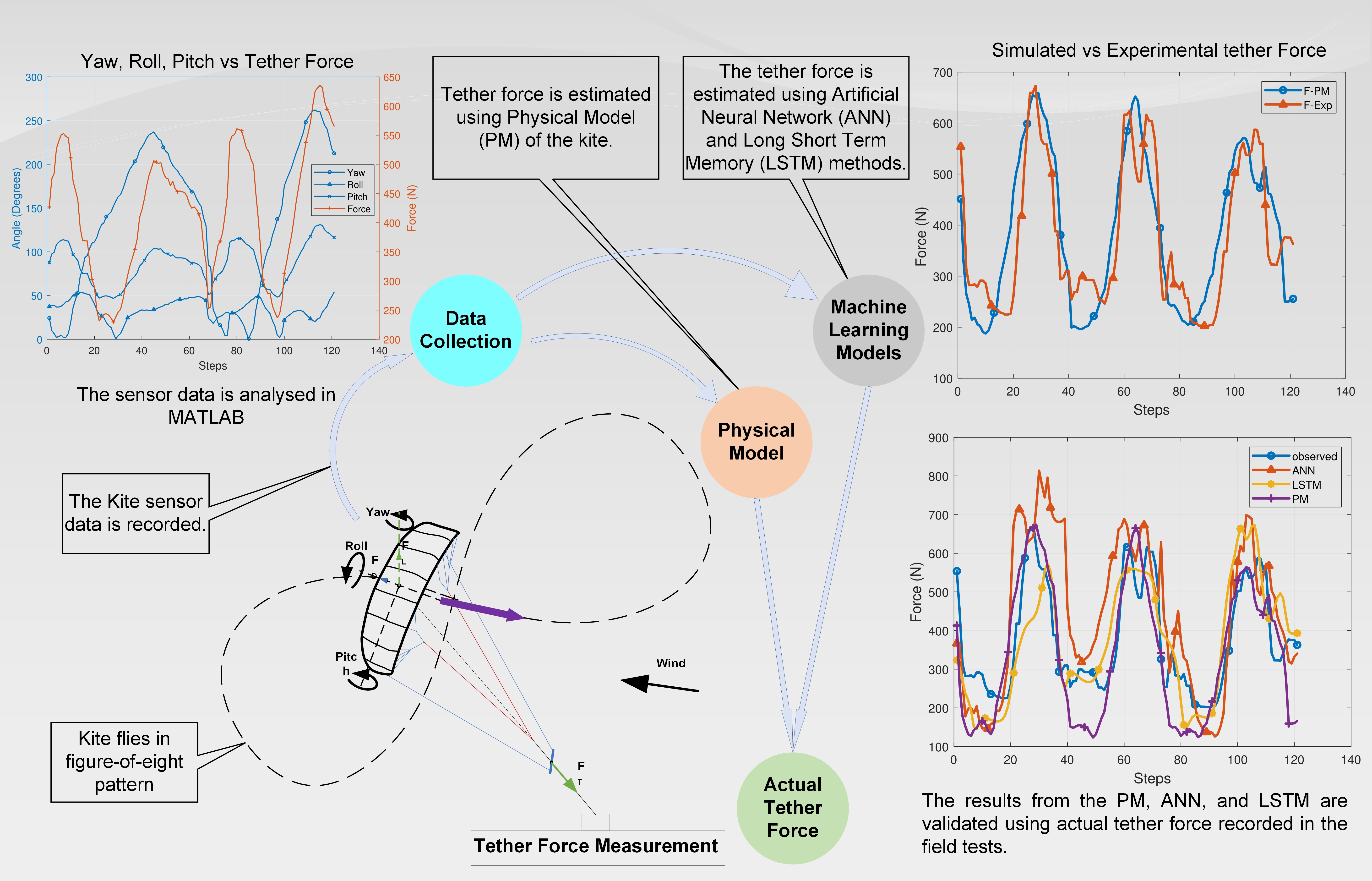
• The proposed approach is based on field data collection, processing, and analysis. The field tests are conducted under steady and turbulent wind conditions, which is explained rigorously.
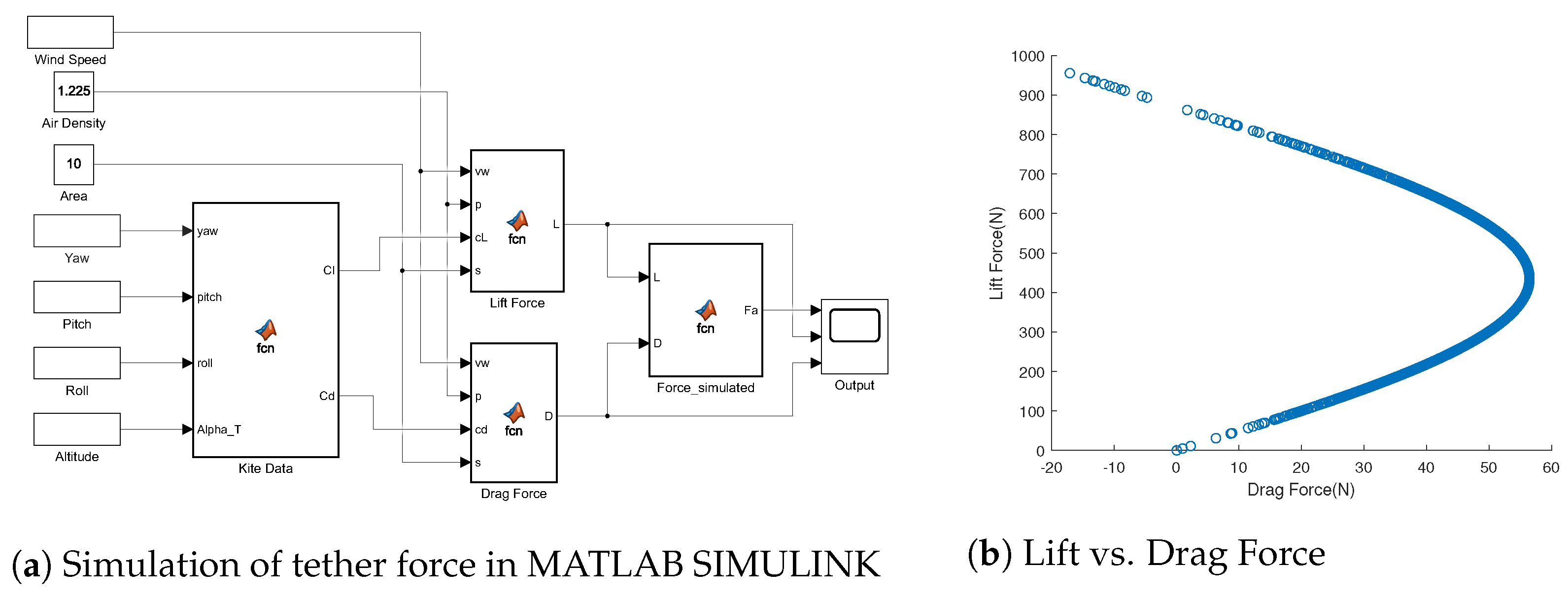
• Tether force estimation using the physical model of a kite is proposed and is simulated using MATLAB SIMULINK.
• Two machine learning models—ANN and LSTM—are trained with the known data from the field tests and the models are tested with unknown data to predict the tether force.
• The proposed methods are experimentally validated and the performance of each method is evaluated.

Section 2 describes the problem description and explains the challenges involved in the experiments. Section 3 describes the tether force estimation methods, the attributes of the experimental setup and its operation in detail. Section 3 also explains the simulation of tether force using a MATLAB SIMULINK environment and the tether force estimation using machine learning techniques. The results are presented in Section 4, which includes the results from the flight tests, simulation results, and experimental validation of the simulated tether force. The conclusions and discussion of this research work are presented in the last Section 5.

2. Problem Description

Estimating the tether force is essential for designing and developing a kite power system. The tether force depends on the kite’s lift coefficient ($C_L$) and drag coefficient ($C_D$). The values of $C_L$ and $C_D$ depend on the angle of attack (AoA), which varies with the kite’s flight (orientation) [31]. The kite’s flight and control are highly nonlinear; hence, modelling the system becomes complicated. In the modelling, assumptions often have to be made to approximate the power output of the system [32]. In many cases, the AoA is assumed to be constant, which makes $C_L$ and $C_D$ constant [33]. In some of the papers, the values of $C_L$ and $C_D$ are assumed to be monotonically increasing with the kite’s trajectory but lack experimental validation [34]. Hence, a simple and accurate approach must be developed to estimate the tether force in the figure-eight trajectory.

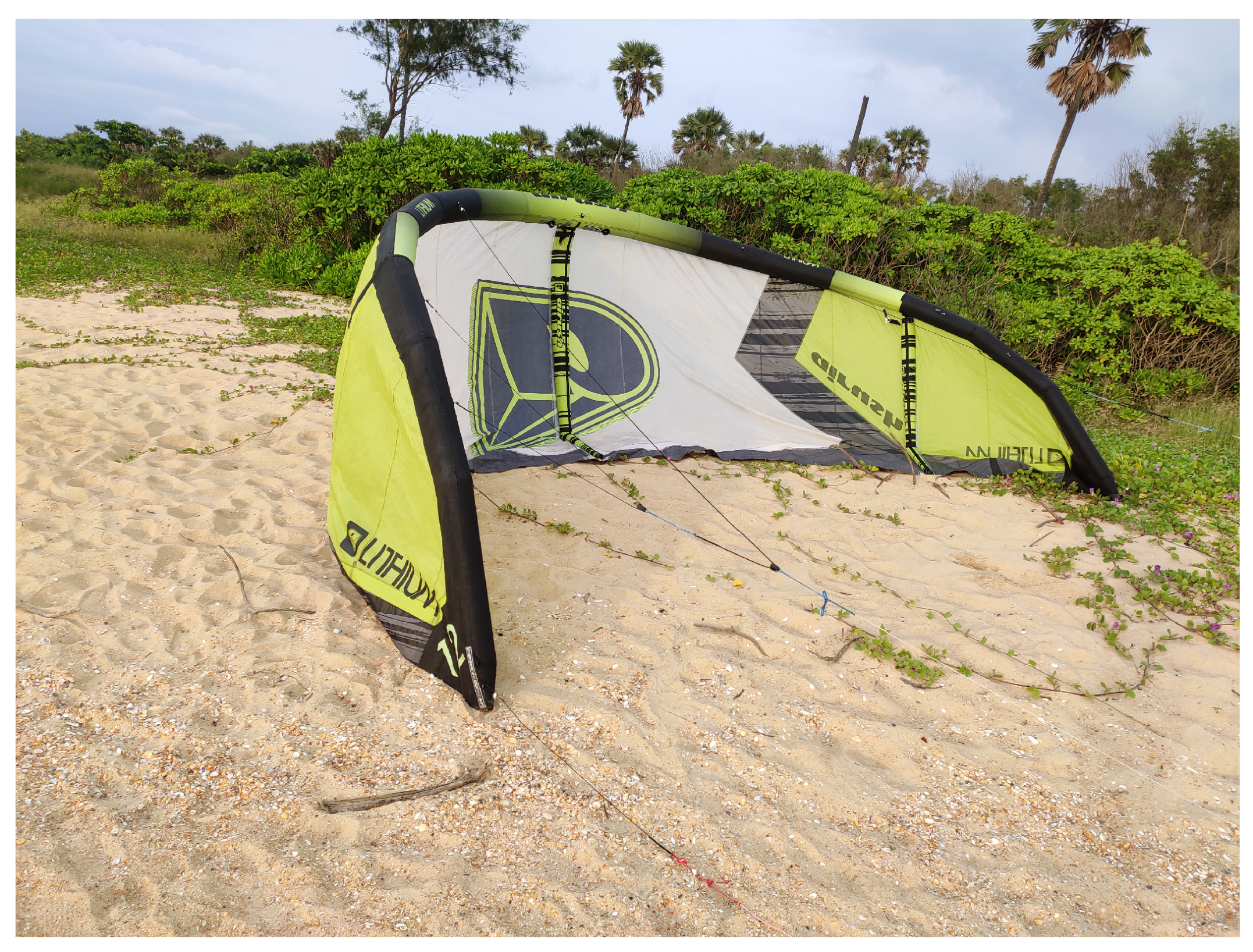
2.1. Kite Constraints

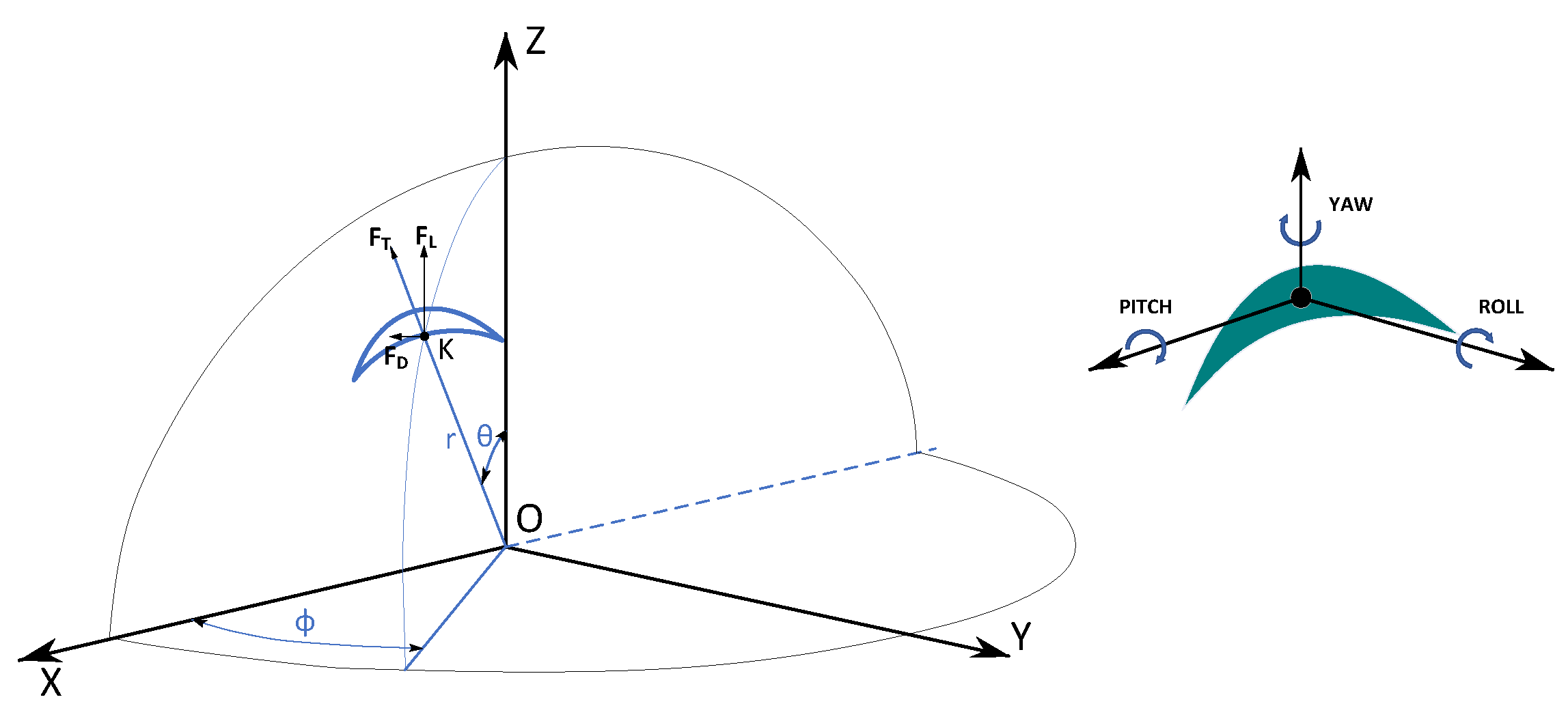
Figure 2 shows the kite’s position and orientation, as well as the AoA of the kite’s trajectory. Figure 2a shows the orientation of the kite in terms of the yaw, roll, and pitch. In the figure, $V_x$ and $V_y$ show the direction of the kite’s travel path and $F_T$ is the tether force measured on the ground. The kite makes an angle with the ground reference called the elevation angle, which is denoted by $\gamma$. In the figure-of-eight trajectory, the kite makes an angle with the reference x-axis called a sweep angle, which is denoted by $\varphi$. $F_L$ denotes the lift force experienced by the kite and the drag force is denoted by $F_D$. Figure 2b shows the AoA of the kite, which is the angle between the kite’s chord line and the relative wind flow. The tether force is measured on the ground, as shown in Figure 2b.

The lift and drag forces can be estimated by finding the relationship between the kite’s orientation and the net aerodynamic force. The orientation of the kite in the Euler form is specified in terms of the yaw, roll, and pitch (YRP) angles, which are related to the measured tether force value from the field tests, to develop the physical model proposed in this paper. There is a negligible sag in the tether for a short tether line, which is a fixed length of 24 m. Therefore, the elevation angle can be calculated using the kite’s altitude.

Hypothesis 1. 

The aerodynamic force of a kite can be estimated by knowing the orientation (YRP) of the kite at a particular altitude and wind speed.

The above hypothesis can be validated using analytical techniques for which the following assumptions are made:

Assumption 1: 

The wind speed at the kite is assumed to be the same as the wind speed on the ground for a short tether length.

Assumption 2: 

The kite is manoeuvred at constant speed in the figure-eight pattern.

Assumption 3: 

The effect of tether drag, sag, and gravity on the net aerodynamic force is negligible.

Assumption 4: 

The tether is assumed to be rigid and straight and the force at the ground station is equal to that at the kite.

2.2. Kite Dynamics

Acquiring accurate orientation data from the kite is challenging. The orientation (YRP) is transmitted to the ground station via wireless communication channels. The measured data should be in quaternions to avoid gimbal lock [35] and the quaternions are converted to the Euler form for calculating the orientation angles. The yaw angle varies from −180 to +180 degrees, the pitch angle varies from −90 to +90 degrees, and the roll angle varies from −180 to +180 degrees. Inertial measurement sensors are required to determine the absolute orientation using an acceleration sensor, gyroscope, and magnetometer [36]. The fusion of the acceleration, gyroscope, and magnetometer values provides the orientation. The quaternions are four signed numbers, including a real number $Q_w$ followed by three imaginary values, $Q_x,Q_y,$ and $Q_z$, representing an object’s rotation. The force calculation of the kite model is in a spherical coordinate system that describes the kite’s orientation in terms of Euler angles. The orientation of the kite in quaternion form is converted into Euler form using the following formula [37]:

$$\left[\begin{array}{c}{\varphi }^{\prime }\\ {\theta }^{\prime }\\ {\psi }^{\prime }\end{array}\right]=\left[\begin{array}{c}atan2(2(Q_w{Q}_x+Q_y{Q}_z),1-2(Q_x^2+Q_y^2))\\ asin\left(2(Q_w{Q}_y+Q_z{Q}_x)\right)\\ atan2(2(Q_w{Q}_z+Q_x{Q}_y),1-2(Q_y^2+Q_z^2))\end{array}\right]$$

(1)

where ${\varphi }^{\prime }$ is the roll of the kite, ${\theta }^{\prime }$ is the pitch of the kite, and ${\psi }^{\prime }$ is the yaw angle of the kite, which are applied in this order [38]. The notation of the YRP angles depends on the sensor (IMU) placement on the kite. In this experiment, the pitch and roll values are interchanged by 90 degrees clockwise according to the sensor placement. Therefore, the pitch values vary from −180 degrees to +180 degrees and the roll values vary from −90 degrees to +90 degrees.

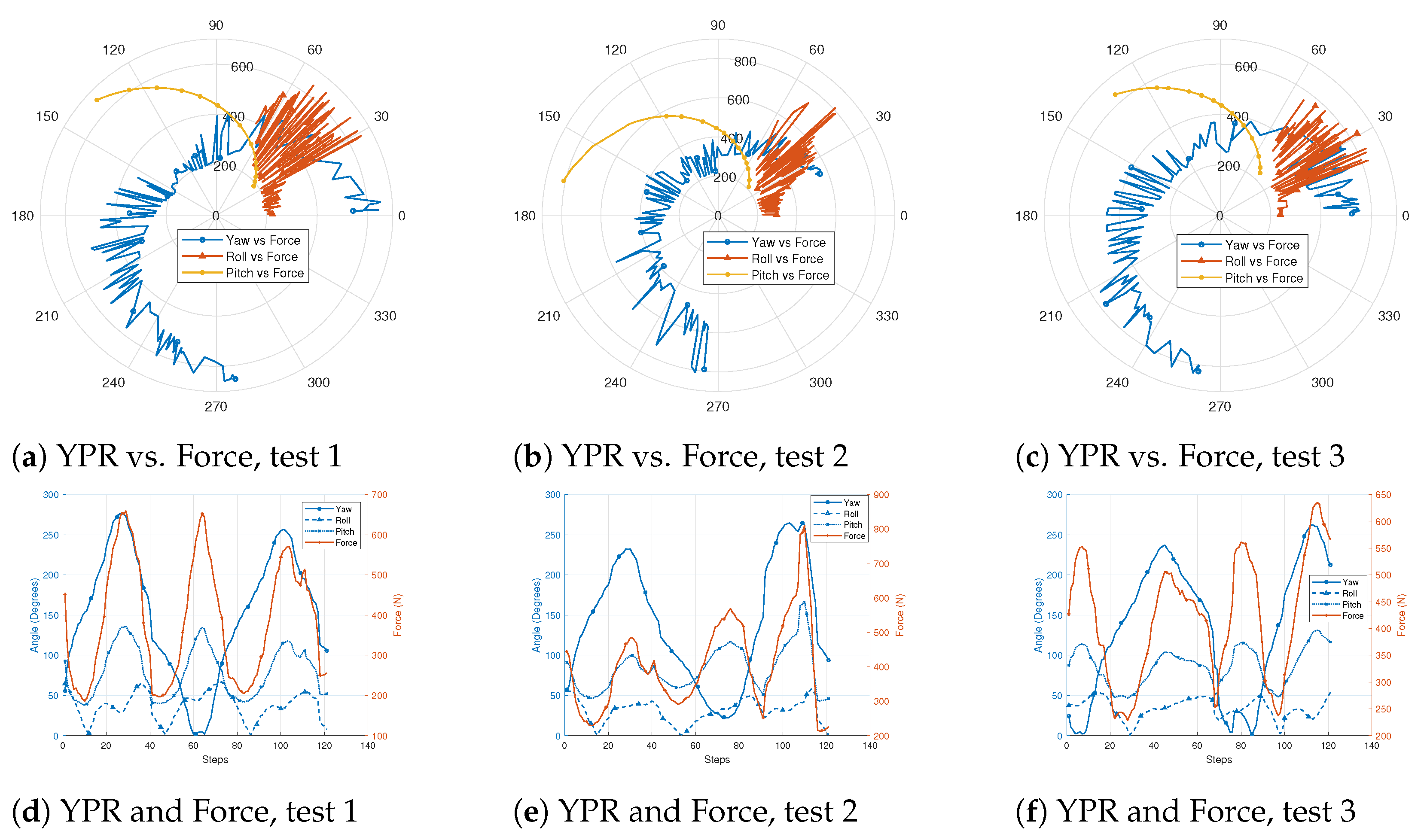
2.3. Kite Field Test Conditions

The field tests were conducted on the shores of the National Institute of Technology Karnataka, Surathkal Beach. Initially, the test was conducted at low wind speeds (3 m/s to 4 m/s) to study the characteristics and learn about flying. Finding the perfect wind conditions to conduct the test was a challenge. Sometimes, there were strong winds and at other times, there was no wind. We experienced a tremendous kite-pulling force that inspired us the most. At first, a rock-mounted anchored safety line was used to hold the kite, but manoeuvring the kite became challenging as the wind direction changed. Later, wood-mounted sandbags were used as a secure platform. The weight of the sandbags was estimated by measuring the tether force from the previous tests.

3. Tether Force Estimation Methods

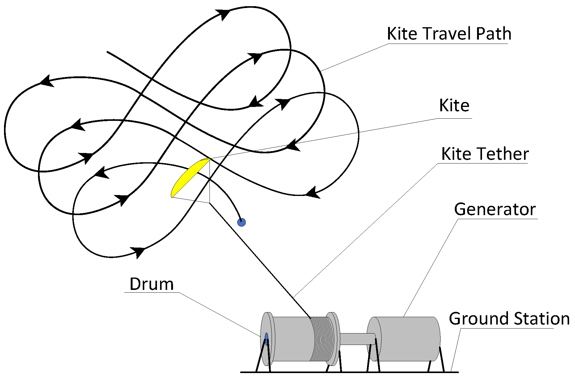
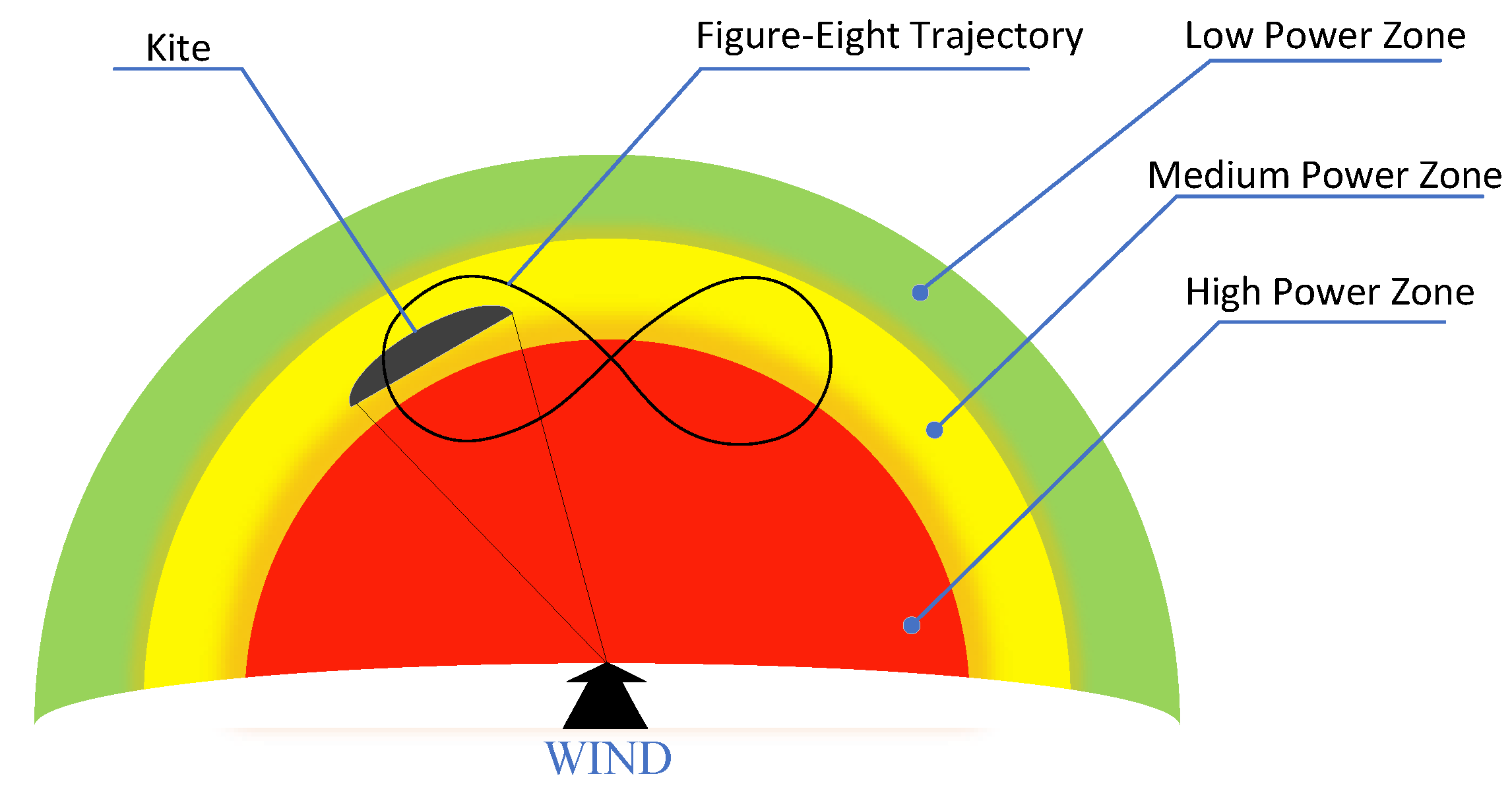
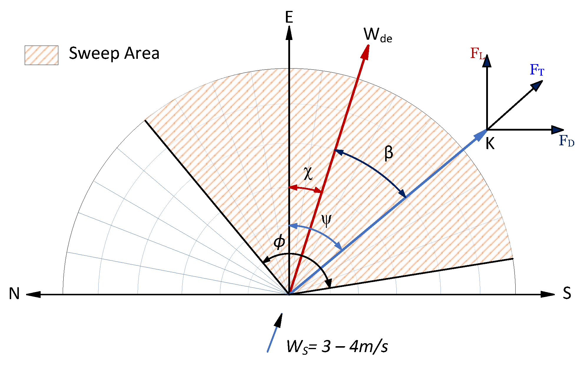
3.1. Wind Window and Crosswind Power

The wind profile plays an essential role in calculating the kite tether force. The “wind window” is an area where a kite can fly in the direction of the wind [12]. When the kite flies in the direction of the wind, it is called a downwind. As shown in Figure 3, if the kite is flown in the maximum power zone, it is called the crosswind zone. When the kite is at the edges of the wind window, the aerodynamic force reduces. The kite is flown in a crosswind zone in the power generation phase to generate maximum power. When the kite reaches the maximum height/length, it returns from the wind window zone and reverts to the initial state, which consumes a fraction of the energy.

3.2. Kite Kinematics and Aerodynamic Force

The kite’s position is represented using a spherical coordinate system, as shown in Figure 4. The proposed method uses a kite reference frame in a spherical coordinate system to represent the kite in the three-dimensional space. Figure 4 shows the kite reference framework in which ‘K’ is the kite’s position, ‘r’ is the tether length, and $\theta$ is the angle between the point K and zenith (Z-axis). The $\varphi$ is the angle between the reference axis (x-axis) and the kite’s orthogonal projection.

The magnitude of the lift and drag forces depends on the AoA, which varies throughout the figure-eight trajectory [39]. The AoA can be estimated by the orientation of the kite under specific wind conditions. The lift and drag forces are estimated by

$$F_L=\frac{1}{2}\rho C_{L}S{v}_w^2$$

(2)

$$F_D=\frac{1}{2}\rho C_{D}S{v}_w^2$$

(3)

where $\rho$ is the air density, $C_L$ and $C_D$ are the lift and drag coefficients, S is the projected area of the kite, and $v_w$ is the wind speed. The resultant aerodynamic force is given by

$$F=\sqrt{{F_L}^2+{F_D}^2}$$

(4)

3.3. Experimental Setup

The following section describes the data collection methodology from the field tests using the experimental setup. Section 3.3.1 through Section 3.3.3 explain the hardware used to acquire the kite’s positional data and the wind data collection on the ground. Section 3.3.4 explains the tether force measurement setup and Section 3.3.5 explains the data logged in the field tests with a plot.

Figure 5 shows the experimental setup used for the measurement of the tether force. Figure 5a shows a pictorial representation and Figure 5b shows the testing of the actual system in the field. The kite used in the experiment was a commercially available Airush Lithium 12 ${\mathrm{m}}^2$ supported leading-edge inflatable (SLEI) kite, as shown in Figure 6.

Table 1. Kite Specifications.

Kite Parameters
No. of Lines	4 lines
Surface Area	12 ${\mathrm{m}}^2$
No. of Struts	3
Canopy Material	Ripstop Nylon
Weight (Deflated)	3.5 kg
Type of kite	Supported leading-edge kite (SLE)

shows the specifications of the kite.

The kite’s measurement system was divided into on-air and on-ground systems. The on-air system consisted of a kite (Figure 6) and its sensor system (Figure 7). The on-ground system consisted of sensors and a data logger system (Figure 8). On the kite, sensors were mounted to measure its orientation, altitude, and location. The measured parameters of the kite were transmitted to the ground using a radio frequency (RF) transmitter module. On the ground, the data were logged after being received from the kite using the RF receiver module. The ground setup consisted of a load cell that measured the force of the kite, a wind speed sensor, and a wind vane to measure the wind direction.

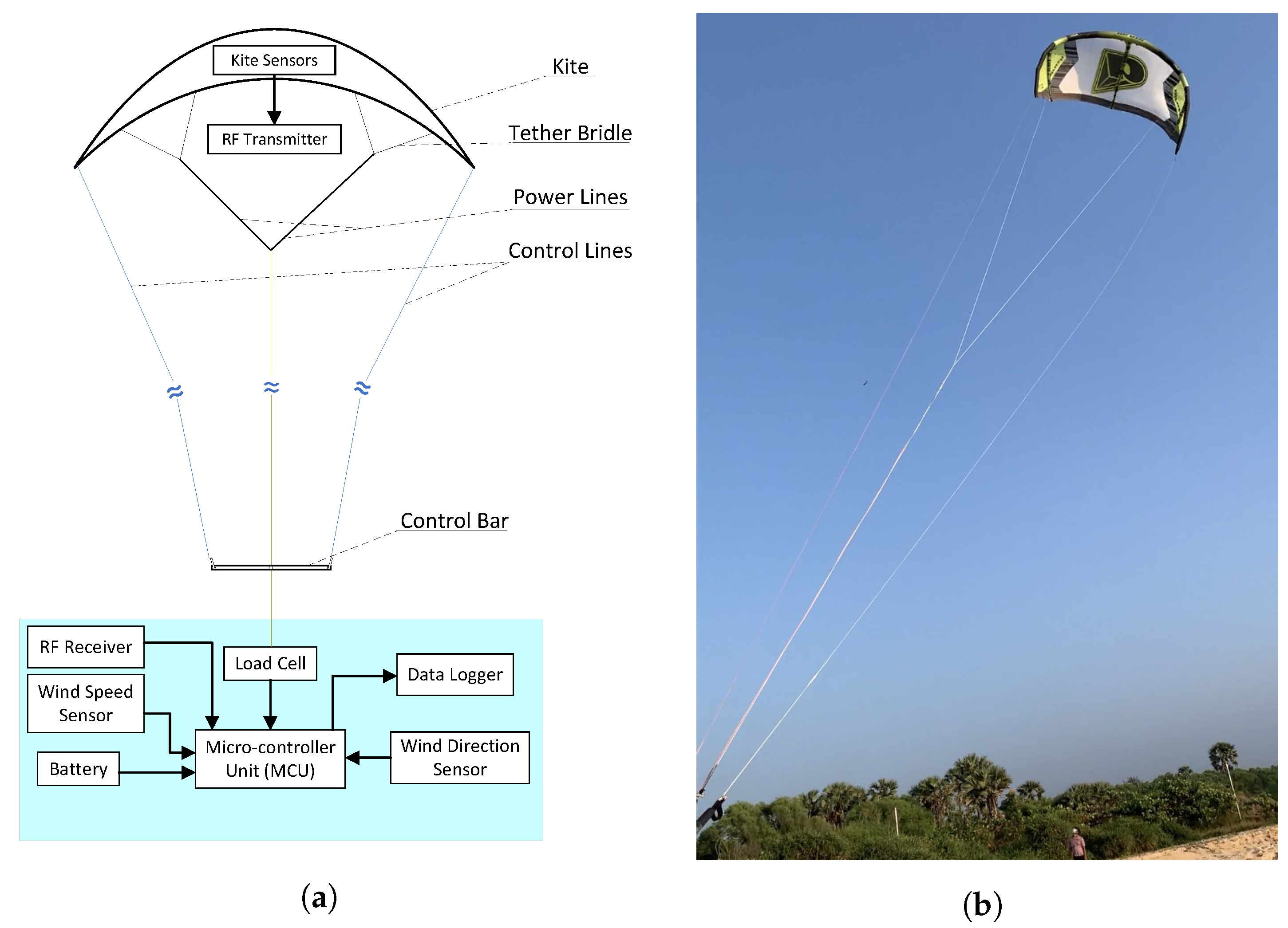
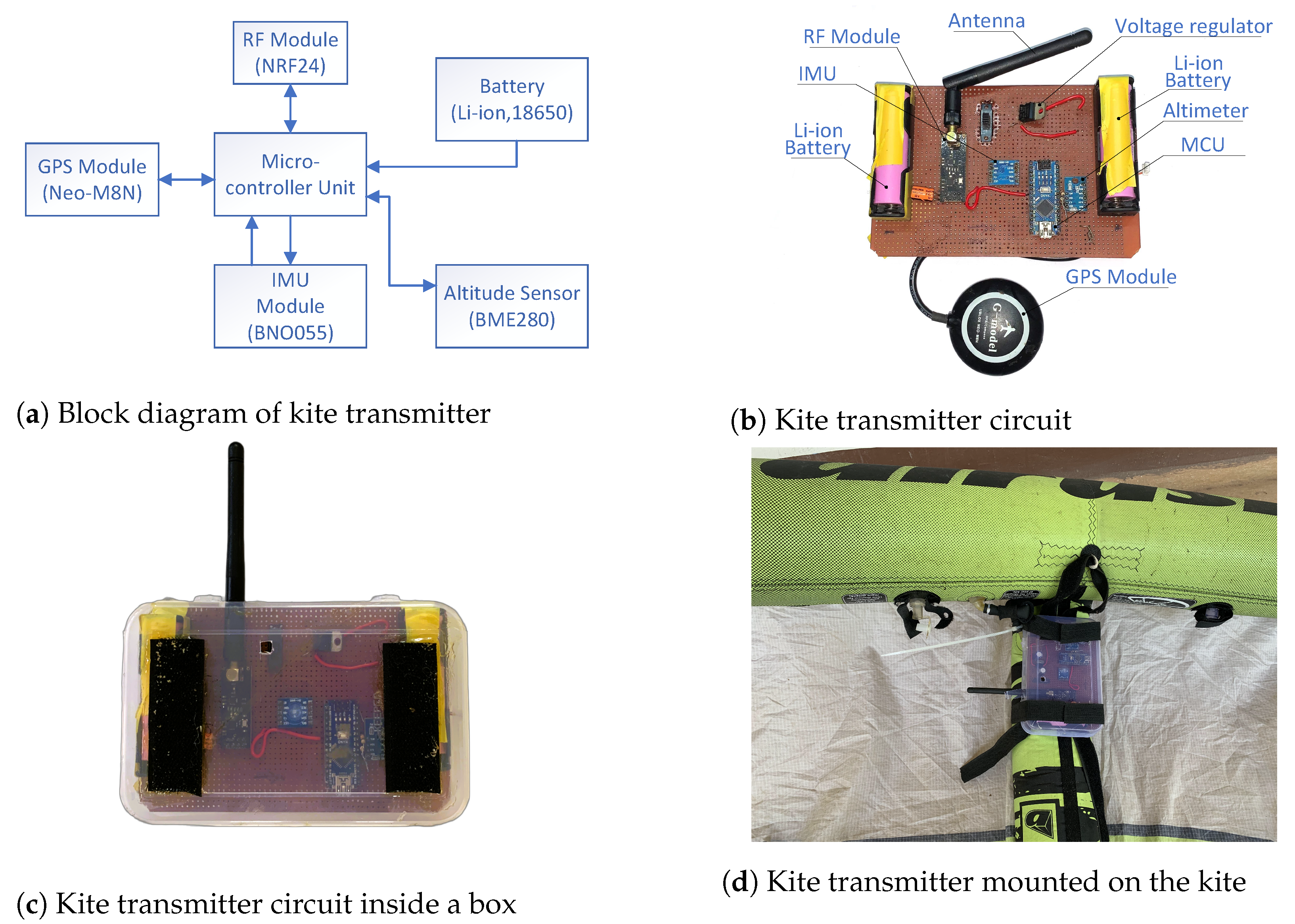
3.3.1. Kite Telemetry System

The proposed tether force estimation approach requires the orientation data of the kite. Since the kite is at a higher elevation, the kite’s orientation data must be transmitted to the ground unit. The kite telemetry system is divided into on-air and on-ground units.

Table 2. Kite telemetry system: on-air kite unit specifications and on-ground kite unit specifications.

Sl No	Part Name	On-Air Kite Unit	On-Ground Kite Unit
1	Wireless Module	NRF24L01 2.4 GHz	NRF24L01 2.4 GHz
2	Micro-Controller Unit (MCU)	ATMEGA328p, 8 bit, 16 MHz, 32 KB flash, 2 KB SRAM, 14 I/O pins	ATMEGA328p, 8 bit, 16 MHz, 32 KB flash, 2 KB SRAM, 14 I/O pins
3	Sensors (20 Hz Sampling)	IMU-BNO055 Altimeter-BME280 GPS—Neo M8N	Loadcell with HX711 ADC Anemometer (Cup type) Wind direction (Encoder)
4	Data Logging	NA	SD card module
5	Power Source	18650 Li-ion battery (Two in series—8 V)	12 V, 7.5 Ah Lead Acid Battery

shows the specifications of the on-air and on-ground units. Figure 7 shows the system setup of the on-air unit.

As shown in Table 2, the micro-controller unit used in this experiment was an ATMEGA328p, which reads the sensor values and sends the values to the ground station via an RF communication link. The Inertial Measurement Unit (IMU) used in this experiment was a BNO055 module with a built-in sensor fusion algorithm. The module can produce rotations in terms of quaternions at a rate of 100 Hz. The kite’s altitude was measured using a barometric pressure sensor module, BME280, which has a sampling rate of 100 Hz. The Global Positioning System (GPS) recorded the kite’s location data, which output the kite’s latitude and longitude at 20 Hz. The sensor data were transmitted to the ground using the NRF24L01+ module, which operates at a 2.4 GHz frequency and has a transmission distance of over 1000 m. The kite’s sensor system was powered by two lithium-ion batteries installed on the PCB.

3.3.2. On-Air Kite Unit

Figure 7a shows a block diagram of the sensor system mounted on the kite. Figure 7b shows the circuit diagram of the transmitter unit. The transmitter unit measured the kite’s orientation, altitude, and location and sent it to the ground station through the RF module. The transmitter PCB was secured inside a plastic container, as shown in Figure 7c, to avoid beach sand and impacts during testing. A box with a sensor unit was attached using velcro, as shown in Figure 7d to measure the flight data.

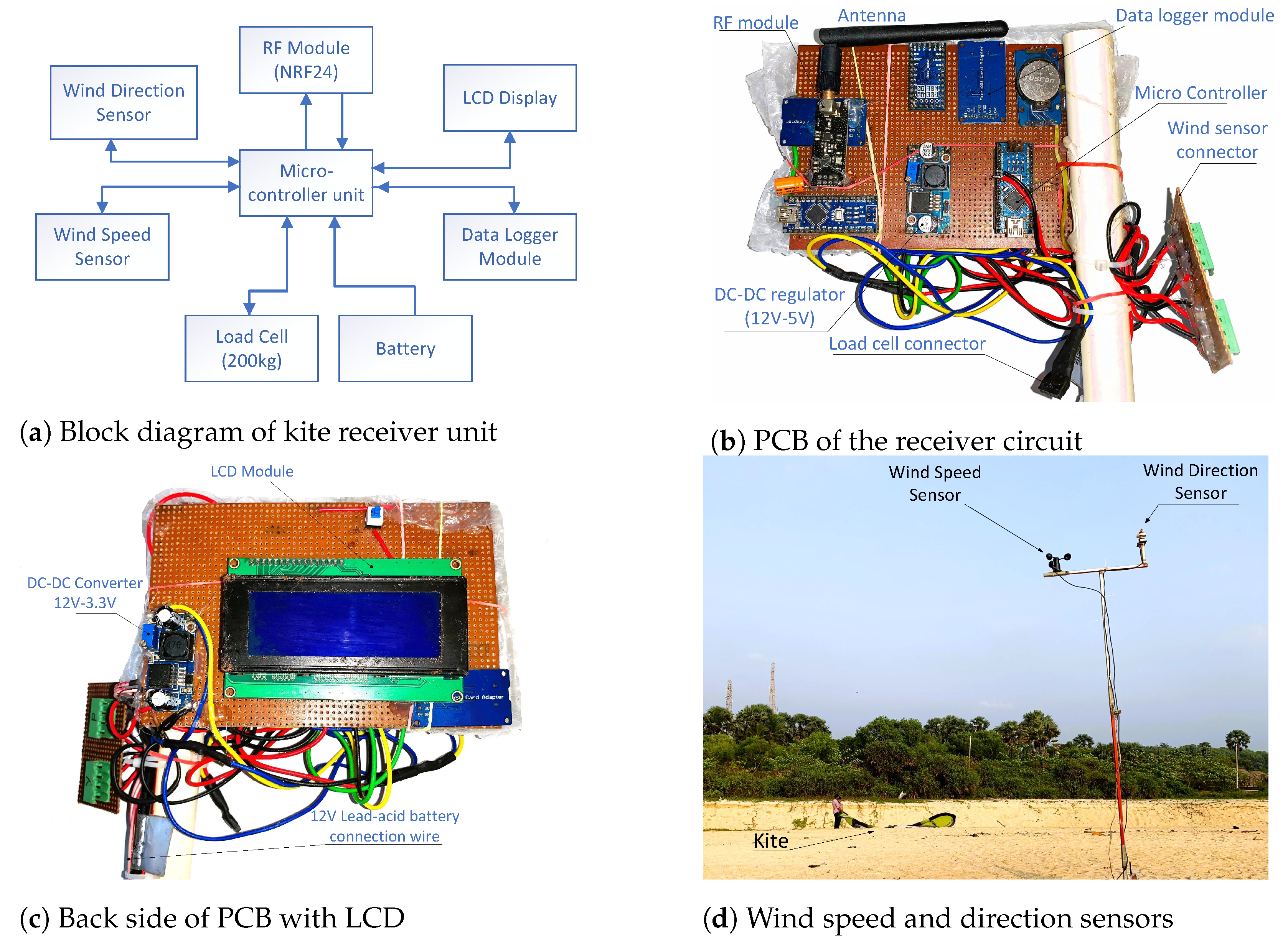
3.3.3. On-Ground Kite Unit

In addition to the kite data receiver circuit, the on-ground unit consisted of wind speed, wind direction, load cell, and data logger modules. Figure 8 shows the system setup of the ground sensor system. A block diagram of the ground unit is shown in Figure 8a. The board was implemented on a PCB, as shown in Figure 8b.

During the field tests, an LCD was installed for visualising the data, and an LCD was installed on which the status of the kite’s data transmission and ground sensor data was displayed, as shown in Figure 8c. The sensors were mounted on the pole to measure the wind speed and direction. The data received from the kite was logged on the ground, which is used to estimate the force using the analytical method.

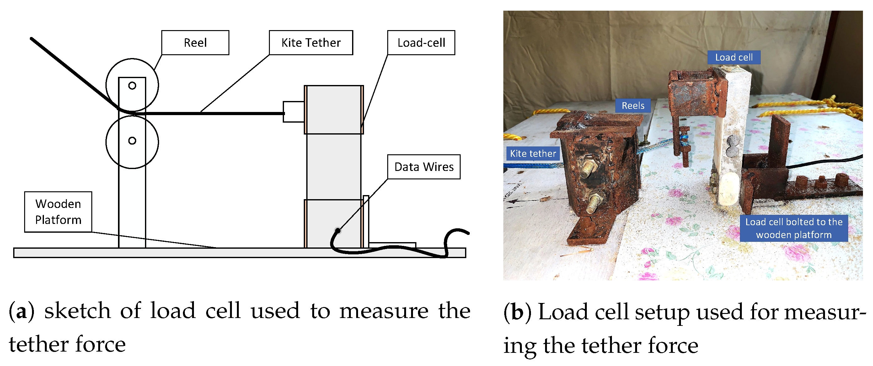
3.3.4. Force Measurement Unit

The force of the fixed- and short-length tethers was equal to the net aerodynamic force of the kite as per the assumptions made in Section 2.1. The force of the tether was measured using a load cell arrangement, as shown in Figure 9. One end of the load cell was anchored to the wooden platform and sandbags and the other was connected to the kite. The output voltage of the load cell changed when the tether exerted a force on the load cell. The subtle changes in voltage were converted to digital form by a 24-bit analogue-to-digital converter (HX711). The digital values obtained from the sensor were then converted to force (Newton).

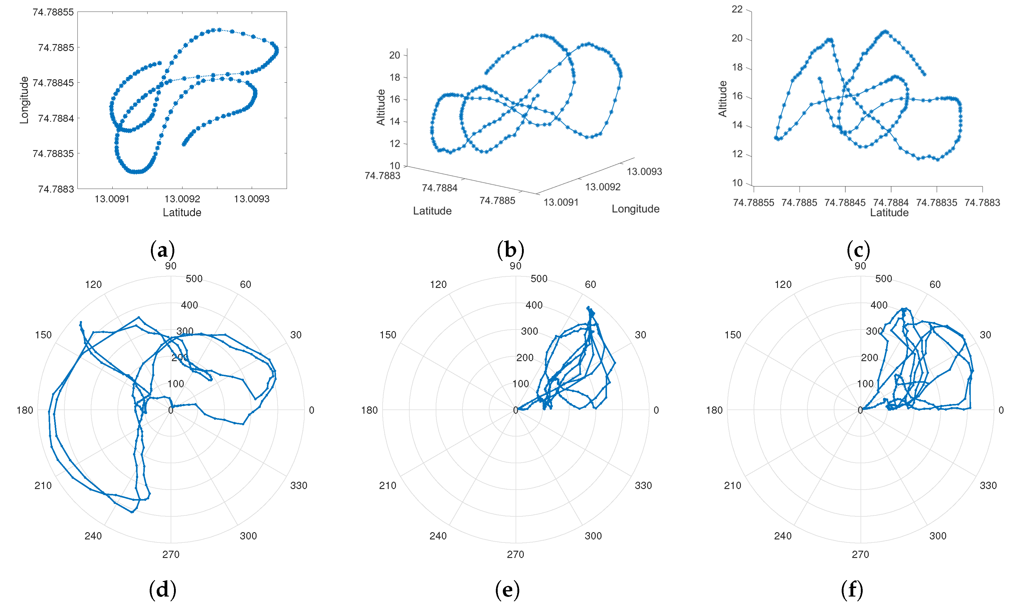
3.3.5. Field Data Collection

The force was estimated using the recorded data from the field tests. Multiple tests were conducted to record the tether force with the kite’s figure-eight trajectory data.

Table 3. Data logged in the field tests consisting of orientation in quaternion form, altitude, GPS data, load-cell values, wind speed, and wind direction.

Data Point	Qw	Qx	Qy	Qz	Altitude (m)	Latitude	Longitude	Load-Cell Analog Value	Wind Speed (m/s)	Wind Direction (Degrees)
1	0.04	−0.36	0.82	0.44	0.43	130091287	747885344	354,420	3.58	15
2	0.06	−0.37	0.82	0.44	0.17	130091287	747885344	611,959	3.63	6
3	0.13	−0.4	0.78	0.47	0.96	130091263	747885311	778,686	3.58	3
4	0.22	−0.44	0.73	0.48	1.95	130091232	747885259	1,012,329	3.58	7
5	0.26	−0.45	0.72	0.46	2.41	130091214	747885219	1,020,015	3.53	13
6	0.3	−0.45	0.73	0.42	4.98	130091167	747885097	955,023	3.55	17
7	0.31	−0.44	0.75	0.4	5.93	130091147	747885017	976,031	3.6	14
8	0.27	−0.41	0.79	0.36	7.14	130091131	747884937	984,059	3.6	9
9	0.2	−0.37	0.85	0.32	8.16	130091119	747884748	947,582	3.63	8
10	0.17	−0.34	0.89	0.27	10.05	130091119	747884655	788,606	3.63	11
11	0.15	−0.32	0.9	0.25	10.66	130091148	747884473	607,128	3.68	13
12	0.16	−0.32	0.9	0.22	12.23	130091164	747884386	550,783	3.7	6
13	0.19	−0.33	0.91	0.18	13.89	130091212	747884234	461,953	3.65	6
14	0.2	−0.34	0.9	0.17	15.53	130091240	747884159	399,323	3.65	15
15	0.2	−0.34	0.91	0.15	16.33	130091300	747884055	405,638	3.65	12

shows the raw data obtained from the field tests, which include the kite orientation data ($Q_w,Q_x,Q_y,Q_z$), altitude of the kite in meters, location of the kite (latitude and longitude), force measurement from the load cell (analogue value), wind velocity (in m/s), and wind direction.

3.4. Kite Tether Force Estimation

According to the hypothesis discussed in Section 2.1, the force from the kite is related to its orientation. The effect of the orientation of the kite on the tether force with varying altitudes and wind speeds was studied. The orientation data of the kite in quaternion form were converted to Euler form, which resulted in the YRP angles, as discussed in Section 2.2. The YRP values changed their signs rapidly, which needed to be filtered to simulate the tether force. The raw values of the yaw (${\psi }_{RAW}$), pitch (${\theta }_{RAW}$), and roll (${\varphi }_{RAW}$) were filtered and converted into positive values. The YRP values were converted by $\psi =|{\psi }_{RAW}|$, $\theta =180-|{\theta }_{RAW}|$, and $\varphi =|{\varphi }_{RAW}|$, respectively.

Figure 10 shows the area swept by the kite in the wind window in the figure-eight trajectory. Although the lift depends on the pitch angle ($\theta$) of the kite, the magnitude of the lift decreased as the kite made an angle $\beta$ with the wind direction vector. The $\beta$ angle, calculated as $|\chi -\psi |$, was zero when the kite tether vector was aligned with the wind direction vector. The $\beta$ angle increased as the kite approached the edges of the wind window, which affected the lift produced by the kite.

Figure 11 shows the kite’s flight path in the experimental field. As the kite moved in a figure-eight trajectory, the force varied according to the position. The GPS and altitude data collected from the field test were used to plot the kite’s trajectory. Figure 11a shows the top view of the kite’s trajectory, Figure 11b shows the front view, and Figure 11c shows the side view of the kite’s trajectory. The figures show that the kite took off from the ground and followed the figure-eight trajectory. Figure 11d–f show the corresponding YRP angles during the trajectory of the kite.

3.4.1. Kite Inclination Effects

The force acting on the kite for a particular wind speed can be split into lift and drag components. The lift components act perpendicular and the drag components act parallel to the wind direction. For an airfoil, the lift and drag components depend on the wind velocity and orientation of the kite in terms of the wind. $C_L$ and $C_D$ change the kite force as per the fundamental aerodynamic Equations (2) and (3) as a function of $\alpha$ (AoA) [40] since the actual measurement of the AoA is difficult and depends on the orientation. $C_L$ and $C_D$ for a thin surface and low-aspect-ratio airfoil [41,42] as a function of $\alpha$ can be written as

$$C_L\approx 2\pi \alpha$$

(5)

$$C_D\approx 1.28\times sin\alpha$$

(6)

The observation made from the field tests was that the $C_L$ is a function of the pitch angle ($\theta$) and sweep angle ($\beta$) and $C_D$ is a function of the pitch angle, sweep angle, and roll angle ($\varphi$). As discussed in Section 3.4, the wind window’s sweep angle and roll angle induce an additional drag as a cosine function. Therefore, by reforming Equations (5) and (6), the equations for $C_L$ and $C_D$ can be written as

$$C_L\approx 2\pi (\theta -\beta )$$

(7)

$$C_D\approx 1.28\times (sin\left(\theta \right)+cos\left(\beta \right)+cos\left(\varphi \right))$$

(8)

3.4.2. Kite Tether Force Estimation Using Physical Model (PM)

Field tests were performed in favourable wind conditions (3 m/s to 6 m/s) to obtain the kite’s orientation data. Hence, the lift and drag forces were estimated by using Equations (7) and (8) in Equations (2) and (3), which yields

$$F_L\approx \frac{1}{2}\rho ·C_L·S{v}_k^2=\frac{1}{2}\rho ·2\pi (\theta -\beta )·S{v}_k^2$$

(9)

$$F_D\approx \frac{1}{2}\rho ·C_D·S{v}_k^2=\frac{1}{2}\rho \times 1.28\times (sin\left(\theta \right)+cos\left(\beta \right)+cos\left(\varphi \right))·S{v}_k^2$$

(10)

As discussed in Section 3.2, the tether force was assumed to be equal to the kite’s force for a tether length of less than 24 m. Hence, the resultant aerodynamic force from Equation (4) yields

$$F_T=\sqrt{{(\frac{1}{2}\rho 2\pi (\theta -\beta )S{v}_k^2)}^2+{\left(\frac{1}{2}\rho 1.28(sin\left(\theta \right)+cos\left(\beta \right)+cos\left(\varphi \right))S{v}_k^2\right)}^2}$$

(11)

Figure 12a shows the simulation of the tether force using the MATLAB SIMULINK environment. The parameters used for the kite were the same as those discussed in Section 3.3. The inputs were imported into SIMULINK in the left blocks, as discussed in Section 3.3.5. The following two lift and drag force blocks were used to compute the lift and drag forces based on Equations (9) and (10). Figure 12b shows the plot of the lift force vs. drag force, which shows a comparison of the lift and drag components of the tether force in the figure-eight trajectory. The resultant aerodynamic force based on Equation (11), which is equal to the tether force, was computed and displayed in the last block, as discussed in Section 4.2.1.

3.4.3. Kite Force Estimation Using Deep Neural Networks

The kite’s power system modelling involves nonlinear dynamics, which depend on the wind and kite parameters. The Deep Neural Network (DNN) technique offers a good solution with noisy data compared to the physical models [19]. The tether force was estimated using Artificial Neural Network (ANN) and Long Short-Term Memory(LSTM) algorithms. The ANN and LSTM model parameters are given in

Table 4. Details of the parameters used in the Deep Learning Models—ANN and LSTM.

S No.	Items	Detail of ANN	Detail of LSTM
1	Target	Tether force	Tether force
2	Input Variable	$Q_w$, $Q_x$, $Q_y$, $Q_z$, Altitude, Wind Speed	$Q_w$, $Q_x$, $Q_y$, $Q_z$, Altitude, Wind Speed
3	Training Parameters	Learning rate: 0.0001, Number of epochs: 1000	Learning rate: 0.0001, Dropout: 0.2, Mini-Batch Size: 8, Number of epochs: 1000
4	Training dataset	Steady Wind Case (30,000) Dynamic Case (30,000)	Steady Wind Case (30,000) Dynamic Case (30,000)
5	Test dataset	Steady Wind Case (1000) Dynamic Case (1000)	Steady Wind Case (1000) Dynamic Case (1000)
6	Network layer	4 (hidden layers)	6 $\left(\begin{array}{c}\hfill \mathrm{F}\mathrm{u}\mathrm{l}\mathrm{l}\mathrm{y}\mathrm{C}\mathrm{o}\mathrm{n}\mathrm{n}\mathrm{e}\mathrm{c}\mathrm{t}\mathrm{e}\mathrm{d}1:\mathrm{B}\mathrm{i}-\mathrm{d}\mathrm{i}\mathrm{r}\mathrm{e}\mathrm{c}\mathrm{t}\mathrm{i}\mathrm{o}\mathrm{n}\mathrm{a}\mathrm{l}\mathrm{L}\mathrm{S}\mathrm{T}\mathrm{M}1:\\ \hfill \mathrm{F}\mathrm{u}\mathrm{l}\mathrm{l}\mathrm{y}\mathrm{C}\mathrm{o}\mathrm{n}\mathrm{n}\mathrm{e}\mathrm{c}\mathrm{t}\mathrm{e}\mathrm{d}2:\mathrm{D}\mathrm{r}\mathrm{o}\mathrm{p}\mathrm{o}\mathrm{u}\mathrm{t}1:\mathrm{B}\mathrm{i}-\mathrm{d}\mathrm{i}\mathrm{r}\mathrm{e}\mathrm{c}\mathrm{t}\mathrm{i}\mathrm{o}\mathrm{n}\mathrm{a}\mathrm{l}\mathrm{L}\mathrm{S}\mathrm{T}\mathrm{M}2:\\ \hfill \mathrm{F}\mathrm{u}\mathrm{l}\mathrm{l}\mathrm{y}\mathrm{C}\mathrm{o}\mathrm{n}\mathrm{n}\mathrm{e}\mathrm{c}\mathrm{t}\mathrm{e}\mathrm{d}3:\mathrm{D}\mathrm{r}\mathrm{o}\mathrm{p}\mathrm{o}\mathrm{u}\mathrm{t}2:\mathrm{F}\mathrm{u}\mathrm{l}\mathrm{l}\mathrm{y}\mathrm{C}\mathrm{o}\mathrm{n}\mathrm{n}\mathrm{e}\mathrm{c}\mathrm{t}\mathrm{e}\mathrm{d}4\end{array}\right)$
7	Number of neurons in each layer	100:50:25:5	100:50:50:25:25:5
8	Training Method	Adam	Adam
9	Loss function	mse	mse
10	Training Type	Regression	Regression

. Figure 13 shows the process of estimating the tether force using the DNN methods. The DNN was fed with 30,000 data points as the input to train the model and 1000 data points to test the model. The values needed to be normalised before being used in the DNN. The orientation data of the kite received in quaternion form were taken as the input, along with the altitude and wind speed.

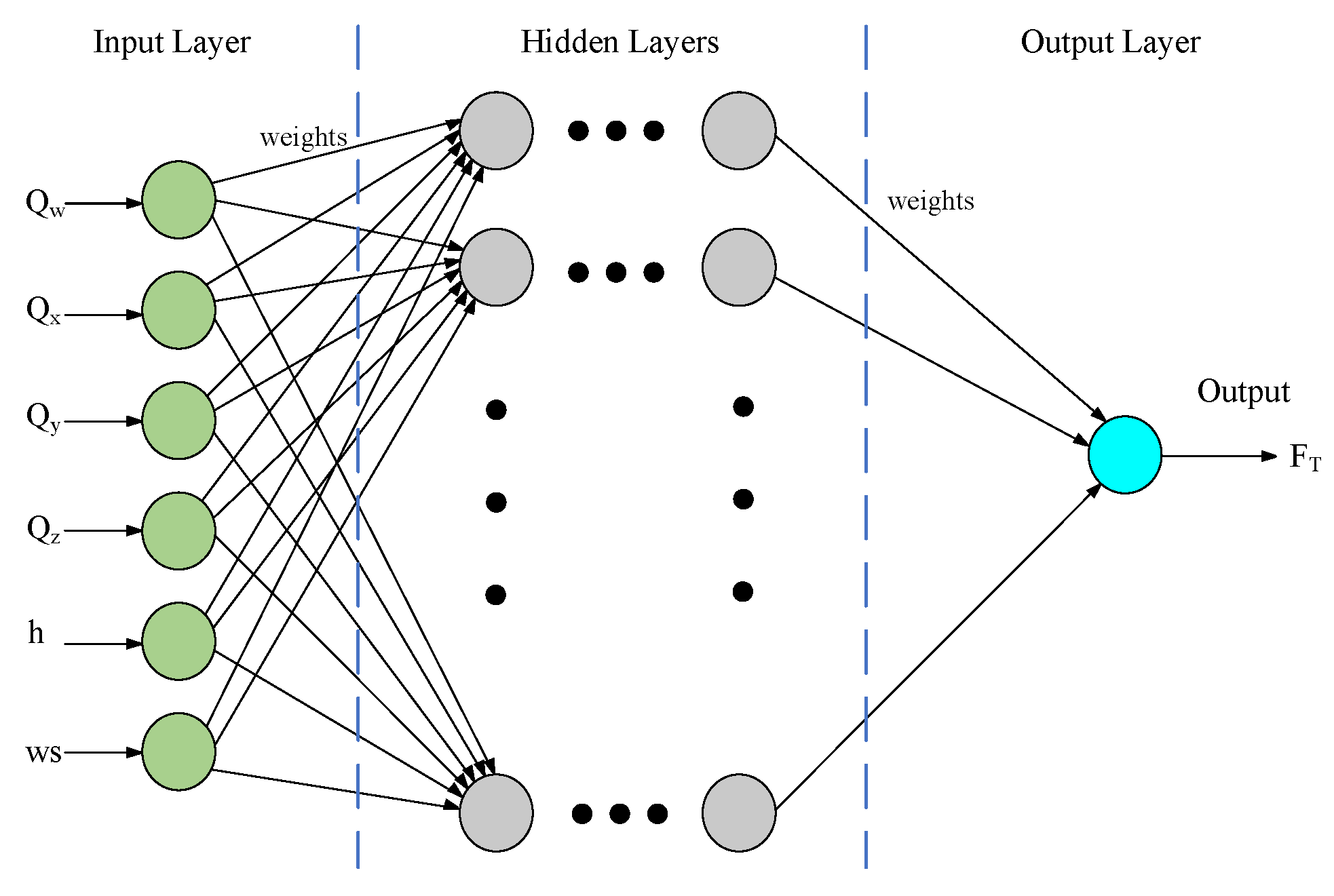
3.4.4. Artificial Neural Network (ANN)

An Artificial Neural Network (ANN) is an interconnection of neurons influenced by the human nervous system [43]. It is a computational approach in which an enormous amount of neurons are inter-connected for parallel processing of the information. ANNs can find a relation between the input and output irrespective of the system’s complexity. Applications of ANNs are growing day by day. In electrical engineering, they are widely used for energy prediction, optimisation, and energy forecasting [44] applications. Figure 14 shows the basic architecture of the ANN in which three layers—input, hidden, and output—are shown. The output is processed by applying weight matrices to the input layers through hidden layers with an activation function. For both the Steady Wind Condition (SWC) and Turbulent Wind Condition (TWC) flight cases, 30,000 data points were given as the training data and 1000 data points were given as the testing data. The neural network had four hidden layers and was trained using the Adam method. ANN computations were performed in the MATLAB coding environment. Table 4 shows the parameters of the proposed ANN approach in which the kite’s orientation in quaternion form, altitude, and wind speed are given as the input matrix and the tether force is obtained as the output, as discussed in Section 4.2.2.

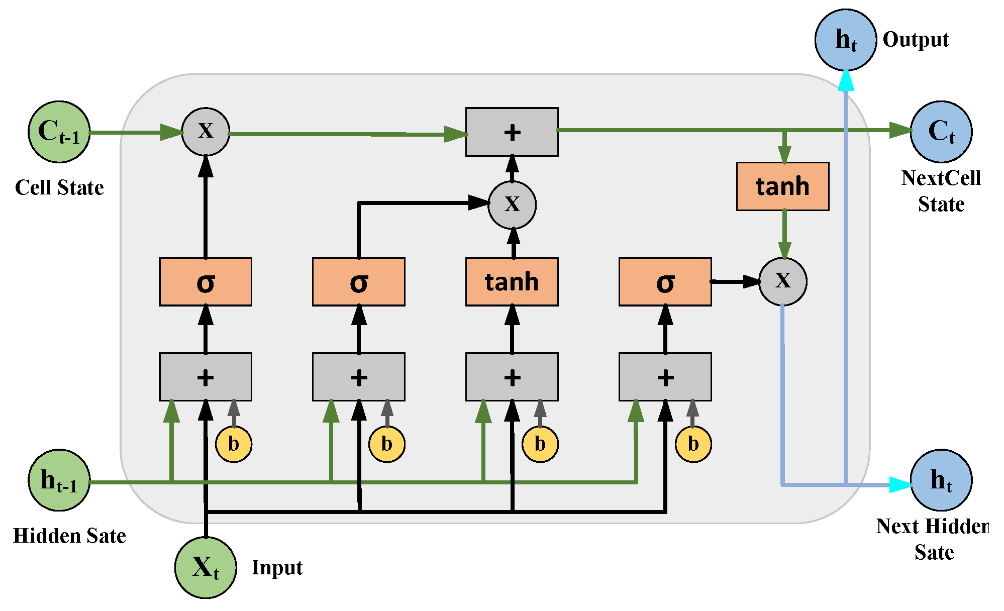
3.4.5. Long Short-Term Memory (LSTM)

The Long Short-Term Memory (LSTM) method is an advancement of the Recurrent Neural Network (RNN), which was developed by Hochreiter and Schmidhuber [45]. The LSTM model consists of sequential blocks called memory cells in which the short-term correlation between the cells is found by comparing each cell state with the adjacent cell states. The LSTM network decides to sustain, define, or update the memory state to evaluate the long-term dependencies [46]. The basic structure of the LSTM network is shown in Figure 15. The parameters involved in the LSTM network are shown in Table 4. The model was fed with the kite’s orientation data, altitude, and wind speed under steady and turbulent wind conditions, with three tests in each case. The LSTM network was trained by a regression-type model with the Adam method and has six network layers. The tether force $F_T$ was the output from the network, as discussed in Section 4.2.3.

4. Results

This section discusses the results of the tether force estimation and validation of the PM, ANN, and LSTM methods using the field test data. The combined analysis of the proposed models was performed by comparing the errors in each test case with the experimental data. Multiple flights were conducted and fed to the models, as discussed for the test data in Section 3.3.5. The models were tested in different test scenarios: steady wind conditions (SWC) and turbulent wind conditions (TWC). In the SWC scenario, the flight parameters (YRP and wind speed) changed gradually, whereas the parameters changed drastically in the TWC scenario. Three flight tests were conducted each for the SWC and TWC.

4.1. PM Simulation Results

The estimation of the tether force through simulations was performed using a MATLAB SIMULINK environment. The kite’s orientation data were loaded as an input matrix in MATLAB and consisted of the yaw, pitch, and roll and wind velocity. The tether force was calculated using Equation (11), as described in Section 3.4.2. The simulation inputs for the two different wind profiles (SWC and TWC) and three separate field test data for each condition were taken as the inputs.

Figure 16 shows the simulation of the tether force under SWC. Figure 16a–c show the polar plots of the YRP angles vs. the tether force for tests 1, 2, and 3, respectively. The plots show the force variation versus the change in the orientation angles (YRP). In Figure 16a–c, it can be seen that the yaw angle varied from $0^{\circ }$ to ${270}^{\circ }$ and the roll angle varied from $0^{\circ }$ to ${70}^{\circ }$, with abrupt changes in the force, which shows a nonlinear relationship between the force and the yaw and roll. We can also observe that the pitch angle varied, following the force in a linear relationship. Figure 16d–f show the time-series plots of the tether force for the corresponding YRP angles for tests 1, 2, and 3, respectively. In the figure, the left y-axis represents the YRP angles in degrees and the right y-axis represents the tether force in Newtons. In Figure 16d–f, it can be seen that the force varied directly with a change in the pitch angle, whereas the yaw and roll angles contributed indirectly to the estimation of the tether force.

The tether force was also simulated under TWC to investigate the effect of abruptly changing the orientation angles and wind velocity in the estimation approach. Three test data sets of the kite’s orientation were used to simulate the tether force under TWC. Figure 17 shows the simulation results of the tether force under TWC where there were abrupt fluctuations in the YRP angles. Figure 17a–c show the polar plots of the YRP angles vs. tether force for test 1, test 2, and test 3, respectively. The figures show that the yaw and roll angles had high variations, whereas the pitch angle variation was acceptable for the force simulation. Figure 17d–f show the time-series plots of the simulated tether force for the corresponding YRP angles for test 1, test 2, and test 3, respectively. The plots show that the orientation angles varied abruptly for the TWC tests. The simulated tether force followed the pitch angle.

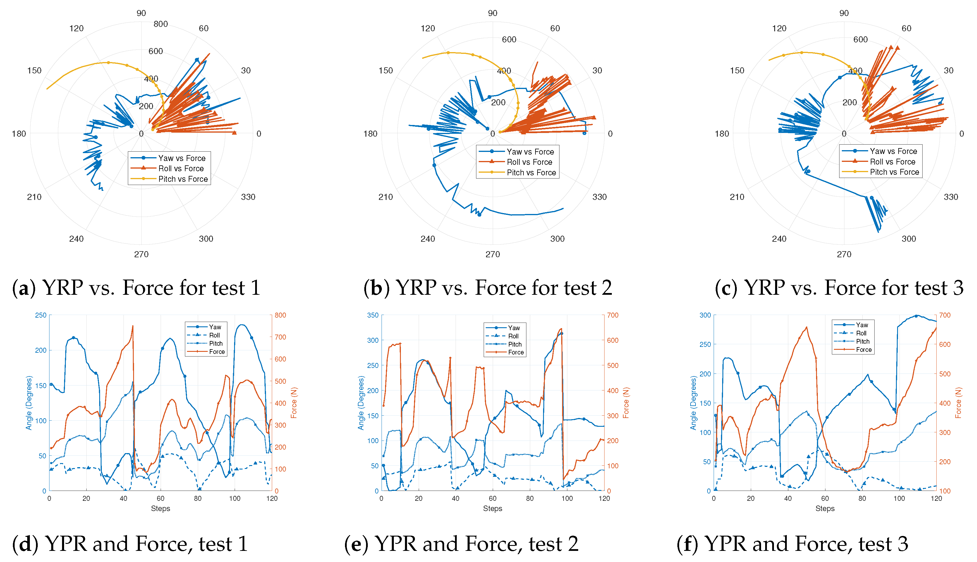
4.2. Tether Force Validation

The flight tests were conducted on the shores of NITK, Surathkal Beach. The tether length of the kite was 24 m and was kept constant. The kite was flown in figure-eight trajectories and the data were recorded for different wind speeds. The recorded kite orientation data with altitude and wind speed were taken as an input matrix in the MATLAB SIMULINK environment to estimate the tether force using the PM, ANN, and LSTM models. The tether force estimated using the above models was validated using experimental tether force data.

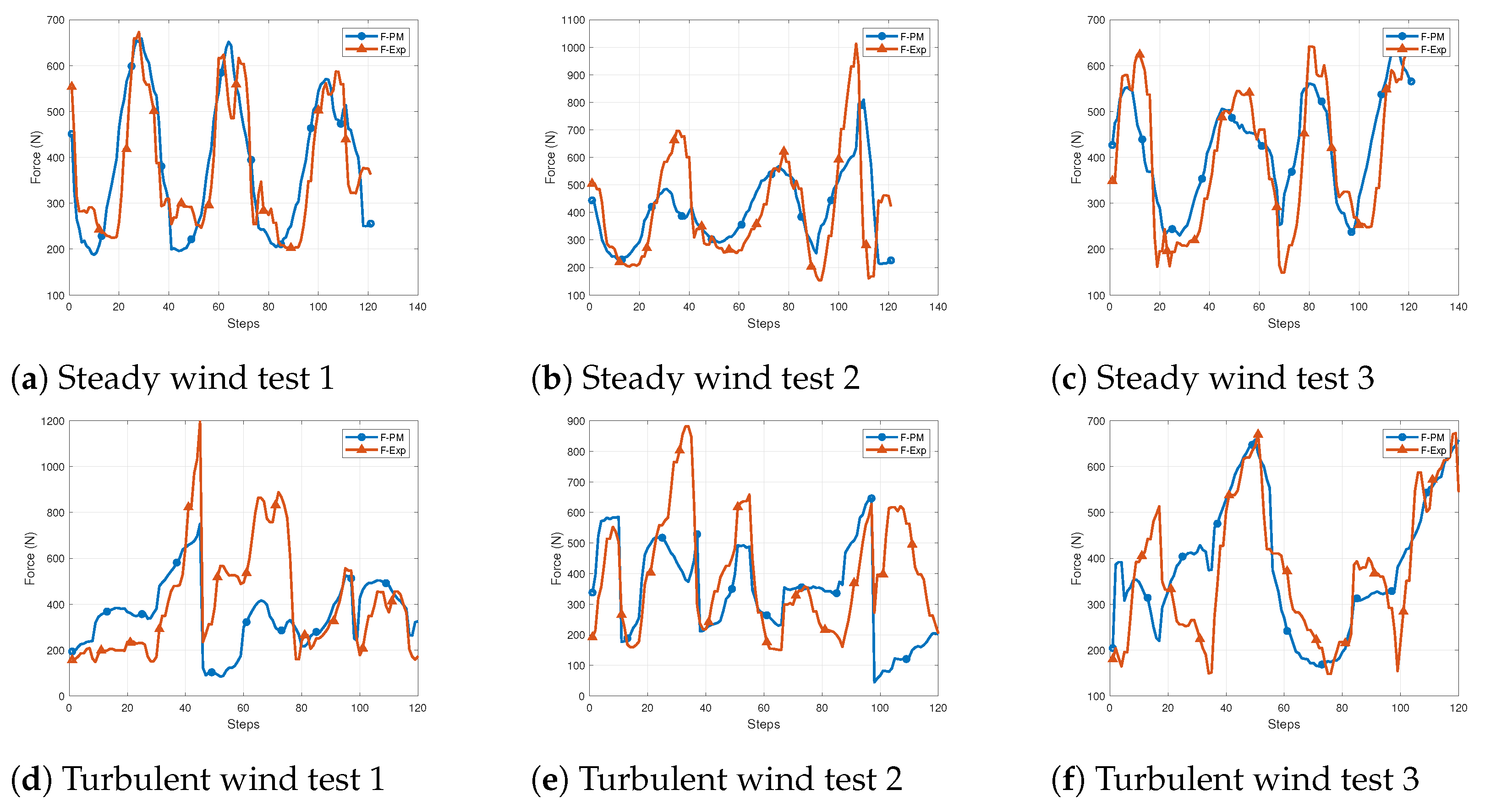
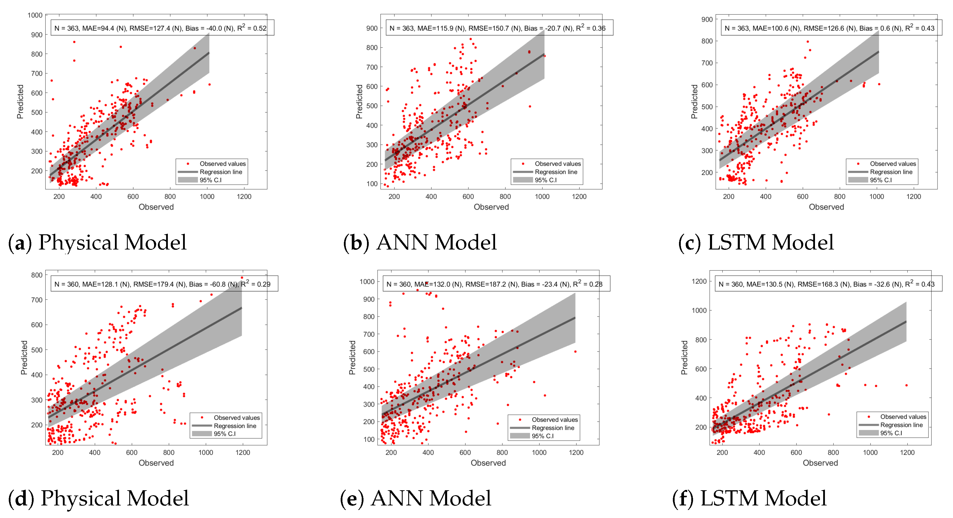
4.2.1. Physical Model (PM) Validation

Figure 18 compares the simulated tether force with the experimental tether force. In the figure, F-PM represents the simulated tether force from the proposed physical model and F-Exp represents the tether force measured in the field tests. Figure 18a–c show a comparison of the tether force from the physical model and the experimental data for tests 1, 2, and 3, respectively, under SWC. In the figures, we can observe that the experimental data varied steadily under SWC and the physical model can estimate the tether force based on the orientation data of the kite. Figure 18d–f show a comparison of the simulated tether force and the experimental force under TWC for tests 1, 2, and 3, respectively. In Figure 18d, we can observe that the tether force in the experimental data changed abruptly due to the TWC and there was a significant error in the simulated tether force. Figure 18e,f also show a significant gap between the simulated force and the actual data from the field tests under TWC. From Figure 18, we can infer that the physical model can perform better for SWC.

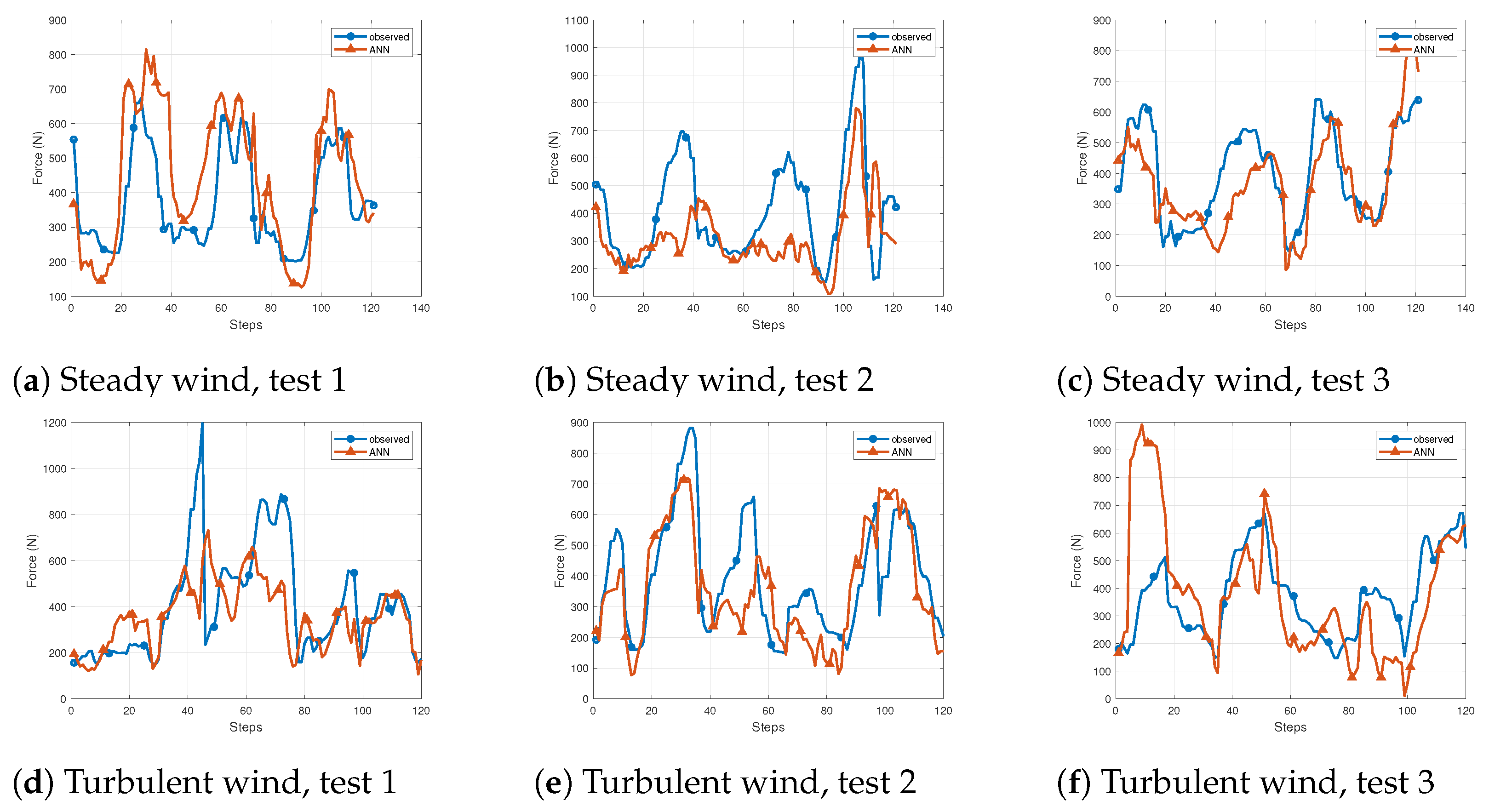
4.2.2. Artificial Neural Network (ANN) Model Validation

The ANN model was trained with the field test data of the SWC and TWC tests. The test results in each case were validated using the experimental data shown in Figure 19. Figure 19a–c show a comparison of the ANN test results and the experimentally observed data for SWC in tests 1, 2, and 3, respectively. From Figure 19a, we can observe that the model estimated the tether force better than the experimentally observed data. Figure 19d–f show the test results of the ANN model compared with the experimental data for TWC in tests 1, 2, and 3, respectively. The prediction of the tether force under SWC using the ANN was similar to that of the PM. For TWC, comparing the results of the PM in Figure 18e with those in Figure 19e, we can observe that the ANN was able to predict better than the PM for TWC. From the results of the ANN model, we can infer that the model similarly estimated the tether force irrespective of steady or turbulent wind conditions.

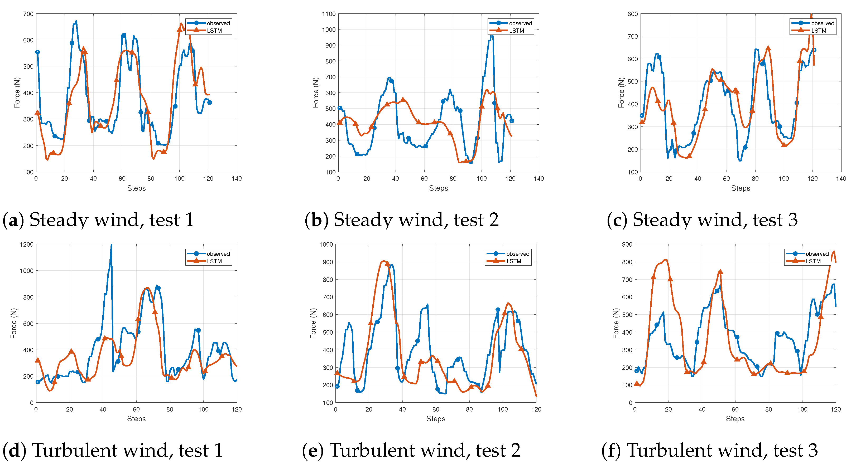
4.2.3. Long Short-Term Memory (LSTM) Model Validation

The LSTM model was trained and tested using the same data points as the physical and ANN models. Figure 20 show the test results of the LSTM model compared with the experimental data. Figure 20a–c show the test results of the LSTM compared with the experimental results for SWC in tests 1, 2, and 3, respectively. From Figure 20a, we can observe that the model performed better and predicted the tether force compared with the experimental data. In Figure 20b, we can observe a deviation in the actual results for test case 2. Figure 20d–f show a comparison of the test results of the LSTM with the experimental data for TWC in tests 1 to 3, respectively. In Figure 20d, we can see that the model was able to estimate the tether force under TWC, except for the spike in the force value. In Figure 20e,f, the estimated values were divergent compared to the experimental values for TWC.

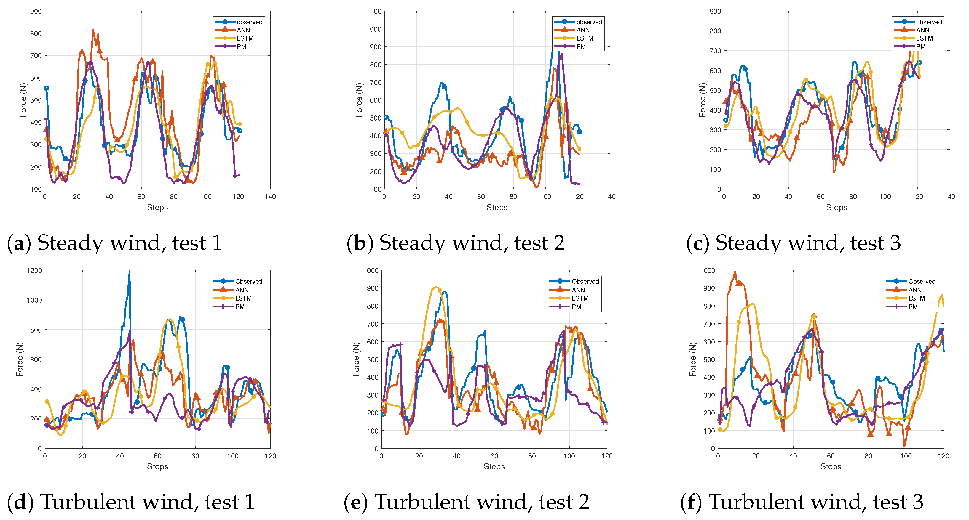
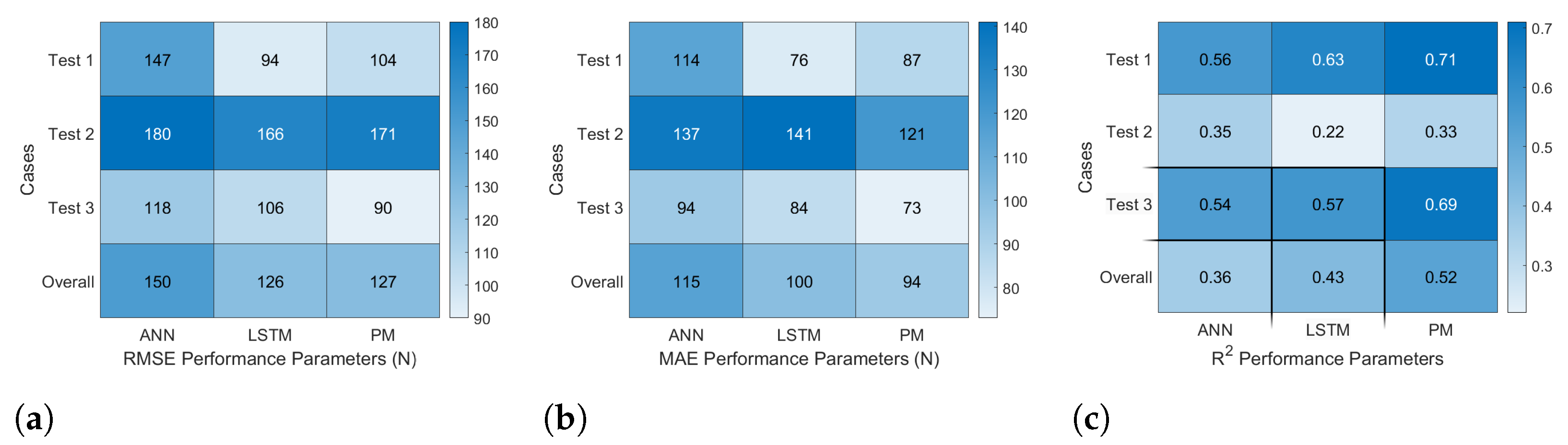
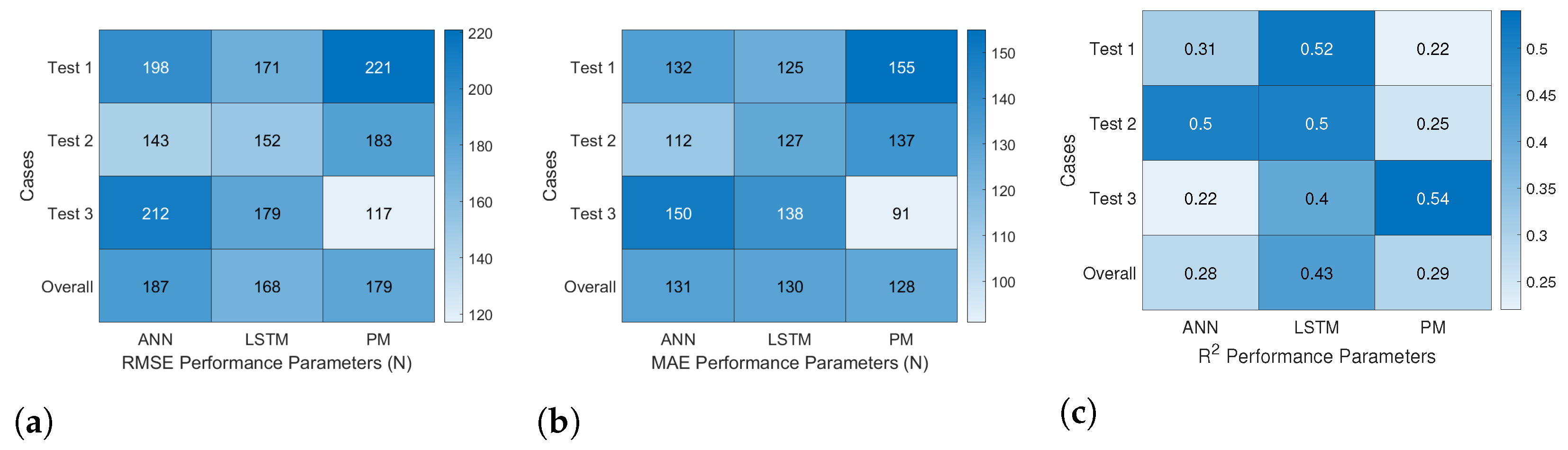
4.2.4. Comparison and Validations of Models

The PM, ANN, and LSTM model results were compared with the actual values measured in the field tests for the combined analysis of the models. Figure 21 shows a comparison of the proposed methods with the experimental values for steady and turbulent wind conditions in three test cases. From Figure 21a–c, we can infer that the physical model performed better in estimating the tether force under SWC in all three test cases. In Figure 21d–f, we can infer that the performance of the PM decreased for TWC as it was susceptible to the noise in the input data, whereas the machine learning methods performed better for TWC.

Figure 22 shows the performance of the PM, ANN, and LSTM models with a linear regression line with a confidence interval (C.I) of 95%. The regression line represents the best fit of the observed values. Figure 22a–c show the scatter plots for 363 data points under SWC and Figure 22d–f show the plots for TWC. In Figure 22a, the performance of the PM under SWC is shown and it can be seen that the observed points are closer to the regression line, which represents the estimated values being closer to the actual values. Figure 22b shows the performance of the ANN model under SWC where the observed values are away from the regression line, indicating that the prediction value was less accurate. Figure 22c shows the performance of the LSTM model under SWC, where we can see that the observed values were better than the ANN model. Figure 22d shows the performance of the PM under TWC. The figure shows that the values are away from the regression line, indicating a reduction in accuracy for TWC. However, the ANN and LSTM model performances, as shown in Figure 22e,f, performed better compared to the PM for TWC.

The error parameters for the three methods were compared with three different error parametrics—the root mean square error (RMSE), mean absolute error (MAE), and R-squared ($R^2$) method.

RMSE Method

This method evaluates the standard deviations in the estimated tether force which are calculated using the equation

$$RMS{E}_{F_T}=\sqrt{\frac{{\sum }_{i=1}^N{(F_{actual}-F_{estimated})}^2}{N}}$$

(12)

where $RMS{E}_{F_T}$ denotes the RMSE of the tether force, $F_{actual}$ is the tether force from the field test, $F_{oredict}$ is the estimated tether force from the machine learning algorithm, and N is the number of non-missing data points.

MAE Method

This method calculates the mean absolute error involved in the tether force measurement. The absolute error is the difference between the actual and estimated tether force. The formula to calculate the MAE for the tether force is given below:

$$MA{E}_{F_T}=\frac{{\sum }_{i=1}^N|F_{actual}-F_{estimated}|}{N}$$

(13)

where $MA{E}_{F_T}$ is the mean absolute error in the tether force and n is the number of errors.

$R^2$ Method

The R-squared method is used to evaluate the best fit or goodness of fit of the expected tether force with the experimental values using the ratio of the sum of squares regression (SSR) and the sum of squares total (SST). The value of R-squared varies from zero to one and has to be closer to one for a better result. The formula to evaluate the error using the $R^2$ method is as follows:

$$R_{F_T}^2=1-\frac{SSR}{SST}=1-\frac{{\sum }_{i=1}^N{(F_{actual}-F_{estimated})}^2}{{\sum }_{i=1}^N{(F_{actual}-\frac{\sum F_{actual}}{N})}^2}$$

(14)

Figure 23 and Figure 24 show the performance analysis of the PM, ANN, and LSTM models for the three tests under SWC and TWC, respectively. In the figures, a lighter cell colour for the RMSE and MAE methods indicates a better estimation of the tether force, whereas for the $R^2$ method, a darker cell colour indicates a better estimation of the tether force.

In Figure 23a, it can be seen that the overall RMSE values of the PM and LSTM models were 127 N and 126 N, respectively, compared to a value of 150 N for the ANN model, which indicates that the PM and LSTM models performed better in SWC. Using the MAE method, the PM had the overall lowest error value of 94 N compared to 115 N and 100 N for the ANN and LSTM, respectively, as shown in Figure 23b. In Figure 23c, it can be seen that the PM had an overall performance score of 0.52, which shows good estimation compared to the scores of 0.36 and 0.43 for the ANN and LSTM methods, respectively, using the $R^2$ method.

Under TWC, the overall RMSE value of the LSTM was 168 N, which was the lowest compared to 187 N and 179 N using the ANN and PM, respectively, as shown in Figure 24a. In Figure 24b, it can be seen that the PM had the overall lowest error value of 128 N, indicating better estimation compared to 131 N and 130 N using the ANN and LSTM methods, respectively, with the MAE method. The $R^2$ method, as seen in Figure 24c, shows that the LSTM method was more accurate, with a value of 0.43, which was the highest among the three, with 0.28 for the ANN and 0.29 for the PM, indicating a better estimation of the tether force in TWC than the ANN and PM.

5. Conclusions

Airborne wind energy has the potential to solve some of the shortcomings of conventional wind turbines. Estimating the tether force is essential for determining the power generation capabilities of the system. The kite is steered in crosswind figure-eight manoeuvres to harvest wind energy. Multiple field tests were conducted in a coastal region to study the kite’s flight dynamics under steady wind conditions (SWC) and turbulent wind conditions (TWC). The test data collected in the field tests were used to estimate the tether force using MATLAB Simulink and Deep Neural Network (DNN) models. The combined analysis of the tether force estimation using the proposed methods was validated using experimental tether force data and the performance of the methods was evaluated using the RMSE, MAE, and $R^2$ methods.

The proposed physical model (PM) had an overall error value of 127 N using the RMSE method and 94 N using the MAE method in estimating the tether force in SWC. However, in turbulent wind conditions, the overall error values increased to 179 N and 128 N using the RMSE and MAE methods, respectively. The PM had a performance index of 0.52 in SWC and 0.29 in TWC using the $R^2$ method, indicating better estimation in SWC than TWC. The proposed ANN model had error values of 150 N and 115 N in SWC using RMSE and MAE methods, respectively, and in TWC, the error values increased to 187 N and 131 N, respectively. The $R^2$ method indicated the change in the error values from 0.36 in SWC to 0.28 in TWC for the ANN method. In the proposed LSTM method, we observed error values of 126 N using the RMSE and 100 N using the MAE in SWC. The error values increased to 168 N using the RMSE and 130 N using the MAE in TWC. Using the $R^2$ method, we observed that the LSTM had an error value of 0.43 in both SWC and TWC, which indicates that the LSTM method had similar performance in the estimation of the tether force in both SWC and TWC.

The PM model relied on the ground-level wind velocity; however, in TWC, the wind velocity at the position of the kite changed rapidly, which made the estimation less accurate. Based on the RMSE method, we can deduce that the LSTM model performed better than the PM and ANN, with overall error values of 126 N and 168 N in SWC and TWC, respectively. The performance of the PM in TWC can be improved by measuring the wind velocity at the kite’s position.

References

1. Olabi, A.G.; Wilberforce, T.; Elsaid, K.; Sayed, E.T.; Salameh, T.; Abdelkareem, M.A.; Baroutaji, A. A review on failure modes of wind turbine components. Energies 2021, 14, 5241. [Google Scholar] [CrossRef]
2. Johansen, K. Blowing in the wind: A brief history of wind energy and wind power technologies in Denmark. Energy Policy 2021, 152, 112139. [Google Scholar] [CrossRef]
3. Caduff, M.; Huijbregts, M.A.; Althaus, H.J.; Koehler, A.; Hellweg, S. Wind power electricity: The bigger the turbine, the greener the electricity? Environ. Sci. Technol. 2012, 46, 4725–4733. [Google Scholar] [CrossRef]
4. DeCarolis, J.F.; Keith, D.W. The economics of large-scale wind power in a carbon constrained world. Energy Policy 2006, 34, 395–410. [Google Scholar] [CrossRef]
5. Meghana, A.; Smitha, B.; Jagwani, S. Technological Advances in Airborne Wind Power: A Review. In Emerging Research in Computing, Information, Communication and Applications; Springer: Singapore, 2022; pp. 349–359. [Google Scholar]
6. Zolfaghari, M.; Azarsina, F.; Kani, A. Feasibility Analysis of Airborne Wind Energy System (AWES) Pumping Kite (PK). J. Adv. Res. Fluid Mech. Therm. Sci. 2020, 74, 133–143. [Google Scholar] [CrossRef]
7. Cherubini, A.; Papini, A.; Vertechy, R.; Fontana, M. Airborne Wind Energy Systems: A review of the technologies. Renew. Sustain. Energy Rev. 2015, 51, 1461–1476. [Google Scholar] [CrossRef] [Green Version]
8. Luchsinger, R.H. Pumping cycle kite power. In Airborne Wind Energy; Springer: Cham, Switzerland, 2013; pp. 47–64. [Google Scholar]
9. Duckworth, R. The application of elevated sails (kites) for fuel saving auxiliary propulsion of commercial vessels. J. Wind Eng. Ind. Aerodyn. 1985, 20, 297–315. [Google Scholar] [CrossRef]
10. Burgin, N.; Wilson, P. The influence of cable forces on the efficiency of kite devices as a means of alternative propulsion. J. Wind Eng. Ind. Aerodyn. 1985, 20, 349–367. [Google Scholar] [CrossRef]
11. Loyd, M.L. Crosswind kite power (for large-scale wind power production). J. Energy 1980, 4, 106–111. [Google Scholar] [CrossRef]
12. Argatov, I.; Rautakorpi, P.; Silvennoinen, R. Apparent wind load effects on the tether of a kite power generator. J. Wind Eng. Ind. Aerodyn. 2011, 99, 1079–1088. [Google Scholar] [CrossRef]
13. Terink, E.; Breukels, J.; Schmehl, R.; Ockels, W. Flight dynamics and stability of a tethered inflatable kiteplane. J. Aircr. 2011, 48, 503–513. [Google Scholar] [CrossRef] [Green Version]
14. Ahmed, M. Optimisation de Contrôle Commande des Systèmes de Génération d’électricité à Cycle de Relaxation. Ph.D. Thesis, Université de Grenoble, Grenoble, France, 2014. [Google Scholar]
15. Ruppert, M.B. Development and Validation of a Real Time Pumping Kite Model. Ph.D. Thesis, Delft University of Technology, Delft, The Netherland, 2012. [Google Scholar]
16. Akberali, A.F.K.; Kheiri, M.; Bourgault, F. Generalized aerodynamic models for crosswind kite power systems. J. Wind Eng. Ind. Aerodyn. 2021, 215, 104664. [Google Scholar] [CrossRef]
17. Rushdi, M.A.; Dief, T.N.; Yoshida, S.; Schmehl, R. Towing test data set of the kyushu university kite system. Data 2020, 5, 69. [Google Scholar] [CrossRef]
18. Borobia-Moreno, R.; Ramiro-Rebollo, D.; Schmehl, R.; Sánchez-Arriaga, G. Identification of kite aerodynamic characteristics using the estimation before modeling technique. Wind Energy 2021, 24, 596–608. [Google Scholar] [CrossRef]
19. LeCun, Y.; Bengio, Y.; Hinton, G. Deep learning. Nature 2015, 521, 436–444. [Google Scholar] [CrossRef]
20. Rushdi, M.A.; Rushdi, A.A.; Dief, T.N.; Halawa, A.M.; Yoshida, S.; Schmehl, R. Power prediction of airborne wind energy systems using multivariate machine learning. Energies 2020, 13, 2367. [Google Scholar] [CrossRef]
21. Orzan, N.; Leone, C.; Mazzolini, A.; Oyero, J.; Celani, A. Optimizing Airborne Wind Energy with Reinforcement Learning. arXiv 2022, arXiv:2203.14271. [Google Scholar]
22. Fechner, U. A Methodology for the Design of Kite-Power Control Systems. Ph.D. Thesis, Delft University of Technology, Delft, The Netherlands, 2016. [Google Scholar]
23. Dief, T.N.; Fechner, U.; Schmehl, R.; Yoshida, S.; Rushdi, M.A. Adaptive flight path control of airborne wind energy systems. Energies 2020, 13, 667. [Google Scholar] [CrossRef] [Green Version]
24. Rushdi, M.; Yoshida, S.; Dief, T.N. Simulation of a Tether of a Kite Power System Using a Lumped Mass Model. In Proceedings of the International Exchange and Innovation Conference on Engineering and Sciences (IEICES), Fukuoka, Japan, 18–19 October 2018; Interdisciplinary Graduate School of Engineering Sciences, Kyushu University: Kyushu, Japan, 2018; pp. 42–47. [Google Scholar]
25. van der Vlugt, R.; Bley, A.; Noom, M.; Schmehl, R. Quasi-steady model of a pumping kite power system. Renew. Energy 2019, 131, 83–99. [Google Scholar] [CrossRef]
26. Oehler, J.; Schmehl, R. Aerodynamic characterization of a soft kite by in situ flow measurement. Wind Energy Sci. 2019, 4, 1–21. [Google Scholar] [CrossRef] [Green Version]
27. Baheri, A.; Vermillion, C. Altitude optimization of airborne wind energy systems: A Bayesian optimization approach. In Proceedings of the 2017 American Control Conference (ACC), Seattle, WA, USA, 24–26 May 2017; pp. 1365–1370. [Google Scholar]
28. Licitra, G.; Koenemann, J.; Bürger, A.; Williams, P.; Ruiterkamp, R.; Diehl, M. Performance assessment of a rigid wing Airborne Wind Energy pumping system. Energy 2019, 173, 569–585. [Google Scholar] [CrossRef]
29. Licitra, G.; Bürger, A.; Williams, P.; Ruiterkamp, R.; Diehl, M. System identification of a rigid wing airborne wind energy system. arXiv 2017, arXiv:1711.10010. [Google Scholar]
30. Dief, T.N.; Fechner, U.; Schmehl, R.; Yoshida, S.; Ismaiel, A.M.; Halawa, A.M. System identification, fuzzy control and simulation of a kite power system with fixed tether length. Wind Energy Sci. 2018, 3, 275–291. [Google Scholar] [CrossRef] [Green Version]
31. Ahmed, M.; Hably, A.; Bacha, S. Power maximization of a closed-orbit kite generator system. In Proceedings of the 2011 50th IEEE Conference on Decision and Control and European Control Conference, Orlando, FL, USA, 12–15 December 2011; pp. 7717–7722. [Google Scholar]
32. Bauer, F.; Kennel, R.M.; Hackl, C.M.; Campagnolo, F.; Patt, M.; Schmehl, R. Drag power kite with very high lift coefficient. Renew. Energy 2018, 118, 290–305. [Google Scholar] [CrossRef] [Green Version]
33. Hummel, J.; Göhlich, D.; Schmehl, R. Automatic measurement and characterization of the dynamic properties of tethered membrane wings. Wind Energy Sci. 2019, 4, 41–55. [Google Scholar] [CrossRef] [Green Version]
34. Houska, B.; Diehl, M. Optimal control for power generating kites. In Proceedings of the 2007 European Control Conference (ECC), Kos, Greece, 2–5 July 2007; pp. 3560–3567. [Google Scholar]
35. Alaimo, A.; Artale, V.; Milazzo, C.; Ricciardello, A. Comparison between Euler and quaternion parametrization in UAV dynamics. Aip Conf. Proc. 2013, 1, 1228–1231. [Google Scholar]
36. Castelino, R.V.; Kashyap, Y. Airborne Manoeuvre Tracking Device for Kite-based Wind Power Generation. In Control Applications in Modern Power System; Springer: Cham, Switzerland, 2021; pp. 497–507. [Google Scholar]
37. Perumal, L. Quaternion and its application in rotation using sets of regions. Int. J. Eng. Technol. Innov. 2011, 1, 35. [Google Scholar]
38. Karduna, A.R.; McClure, P.W.; Michener, L.A. Scapular kinematics: Effects of altering the Euler angle sequence of rotations. J. Biomech. 2000, 33, 1063–1068. [Google Scholar] [CrossRef]
39. Dadd, G.M.; Hudson, D.A.; Shenoi, R. Determination of kite forces using three-dimensional flight trajectories for ship propulsion. Renew. Energy 2011, 36, 2667–2678. [Google Scholar] [CrossRef]
40. Center, N.G.R. Kite Inclination Effects. 2005. Available online: https://www.grc.nasa.gov/www/k-12/VirtualAero/BottleRocket/airplane/kiteincl.html (accessed on 20 January 2022).
41. Paiva, L.T.; Fontes, F.A. Optimal control of underwater kite power systems. In Proceedings of the 2017 International Conference in Energy and Sustainability in Small Developing Economies (ES2DE), Funchal, Portugal, 10–12 July 2017; pp. 1–6. [Google Scholar]
42. Hobbs, S. A Quantitative Study of Kite Performance in Natural Wind with Application to Kite Anemometry. Ph.D. Thesis, Cranfield University, Bedford, UK, 1986. [Google Scholar]
43. Wang, S.C. Artificial neural network. In Interdisciplinary Computing in Java Programming; Springer: Cham, Switrzerland, 2003; pp. 81–100. [Google Scholar]
44. Ahmad, A.S.; Hassan, M.Y.; Abdullah, M.P.; Rahman, H.A.; Hussin, F.; Abdullah, H.; Saidur, R. A review on applications of ANN and SVM for building electrical energy consumption forecasting. Renew. Sustain. Energy Rev. 2014, 33, 102–109. [Google Scholar] [CrossRef]
45. Schmidhuber, J.; Hochreiter, S. Long short-term memory. Neural. Comput. 1997, 9, 1735–1780. [Google Scholar]
46. Greff, K.; Srivastava, R.K.; Koutník, J.; Steunebrink, B.R.; Schmidhuber, J. LSTM: A search space odyssey. IEEE Trans. Neural Netw. Learn. Syst. 2016, 28, 2222–2232. [Google Scholar] [CrossRef] [PubMed]
Figure 1. Kite power generation technique: kite travels in a figure-eight trajectory, which pulls the tether wound on the drum and rotates the generator to produce electric power.
Remotesensing 14 06111 g001
Figure 2. Kite’s position and orientation represented in the spherical coordinate system and the forces experienced by the kite [26]. (a) Kite’s orientation and position. (b) Angle of attack of the kite.
Remotesensing 14 06111 g002
Figure 3. Wind window: an imaginary boundary in which the kite can be flown to produce power; the red area indicates the maximum power zone, the yellow area shows the moderate power zone, and the green area indicates the low power zone.
Remotesensing 14 06111 g003
Figure 4. Kite reference frame [25]: The left figure shows the position of the kite at point K in a three-dimensional plane with the forces acting on the kite. The right figure shows the orientation of the kite in terms of the Euler form.
Remotesensing 14 06111 g004
Figure 5. Experimental setup: (a) pictorial representation of the system used for estimating the tether force with a block diagram of the system, (b) Actual experimental setup used in the experimental tests.
Remotesensing 14 06111 g005
Figure 6. Airush Lithium 12 m 2 Kite.
Remotesensing 14 06111 g006
Figure 7. Sensor system on the kite: (a) block diagram of the system, (b) PCB implementation of the sensor system, (c) PCB enclosed within the box for protection, (d) Sensor system installed on the kite using velcro.
Remotesensing 14 06111 g007
Figure 8. Sensor system on the ground: (a) Block diagram of the kite data receiver system on the ground, (b) Implementation of the sensor data receiver circuit in the PCB, (c) Back side of the PCB with LCD, (d) Wind speed and direction sensors at the testing site.
Remotesensing 14 06111 g008
Figure 9. Measurement of tether force using lad-cell, (a) shows the pictorial representation of the setup, (b) shows the actual setup mounted on the wooden board in which the tether is passed through the pulleys.
Remotesensing 14 06111 g009
Figure 10. Wind window with shaded area indicating area swept by the kite in the figure-eight trajectory ( ϕ degrees); W d e represents the wind direction vector; K represents kite tether vector; N, E, and S are the north, east, and south reference vectors; χ is the angle between east and W d e ; ψ is the angle between east and the kite tether vector; β is the angle between W d e and the kite tether vector.
Remotesensing 14 06111 g010
Figure 11. The figure-eight trajectory followed by the kite during the test. The GPS and altitude data were used to plot the trajectory of the kite in 3 dimensions. (a) Top view: lat vs. lon. (b) 3D view: lat-lon vs. altitude. (c) Side view: lat vs. altitude. (d) Yaw vs. Force. (e) Roll vs. Force. (f) Pitch vs. Force.
Remotesensing 14 06111 g011
Figure 12. Simulation of tether force in MATLAB SIMULINK: (a) From left, the data from the field test are given as a numeric matrix and the kite’s data block filters the data to calculate the lift and drag forces; the force–simulated block calculates the tether force. (b) Shows a plot of the lift force vs. drag force from the simulated tether force.
Remotesensing 14 06111 g012
Figure 13. The flow of the estimation of the tether force using the DNN methods: The field test data were imported to the models and then normalised so that they could be used in the ANN and LSTM models; the predicted data in the normalised form were then inverted to the actual values; the performance was evaluated using the RMSE, MAE, and R 2 methods.
Remotesensing 14 06111 g013
Figure 14. The basic architecture of the ANN: the input layer is fed with the kite’s orientation data on altitude and wind speed; there are four hidden layers between the input and output and the output of the ANN was the tether force ( F t ).
Remotesensing 14 06111 g014
Figure 15. The basic structure of a Long Short-Term Memory (LSTM) unit: X t is the current input; h t 1 is the last output; C t 1 is the memory from the last LSTM unit; h t is the current output; C t is the next cell state; ’b’ is the bias; ’ σ ’ block is a sigmoid layer; ’ t a n h ’ block is a tanh layer; ’×’ and ’+’ are the scaling and addition operators, respectively.
Remotesensing 14 06111 g015
Figure 16. Tether force simulation for three test cases: (ac) polar plots of the YRP vs. force; the sweep represents the angles ( 0 to 360 ) and the magnitude represents the tether force, (df) time-series plots of the YRP and the tether force under the steady wind conditions.
Remotesensing 14 06111 g016
Figure 17. Tether force simulation for three test cases: (ac) polar plots of the YRP vs. force; the sweep represents the angles ( 0 to 360 ) and the magnitude represents the tether force, (df) time-series plots of the YRP and the tether force under turbulent wind conditions.
Remotesensing 14 06111 g017
Figure 18. Validation of the physical model with the experimental data: (ac) steady wind conditions, (df) turbulent wind conditions.
Remotesensing 14 06111 g018
Figure 19. Experimental validation of predicted tether force from ANN: (ac) test results for steady wind conditions, (df) test results for turbulent wind conditions.
Remotesensing 14 06111 g019
Figure 20. LSTM model test results comparison with the experimental data: (ac) steady wind condition data for the three tests, (df) turbulent wind condition data for the three tests.
Remotesensing 14 06111 g020
Figure 21. Combined analysis of tether force estimation methods–physical, ANN, and LSTM methods: (ac) the three tests under steady wind conditions, (df) the three tests under turbulent wind conditions.
Remotesensing 14 06111 g021
Figure 22. Scatter plots of the physical, ANN, and LSTM models: (ac) the performance of the models under steady wind conditions, (df) the performance of the models under turbulent wind conditions.
Remotesensing 14 06111 g022
Figure 23. Performance analysis of PM, ANN, and LSTM models under steady wind conditions: (a) RMSE method, (b) MAE method, (c) R 2 method.
Remotesensing 14 06111 g023
Figure 24. Performance analysis of PM, ANN, and LSTM models under turbulent wind conditions: (a) RMSE method, (b) MAE method, (c) R 2 method.
Remotesensing 14 06111 g024