Zero-Shot Remote Sensing Image Dehazing Based on a Re-Degradation Haze Imaging Model

Abstract

Image dehazing is crucial for improving the advanced applications on remote sensing (RS) images. However, collecting paired RS images to train the deep neural networks (DNNs) is scarcely available, and the synthetic datasets may suffer from domain-shift issues. In this paper, we propose a zero-shot RS image dehazing method based on a re-degradation haze imaging model, which directly restores the haze-free image from a single hazy image. Based on layer disentanglement, we design a dehazing framework consisting of three joint sub-modules to disentangle the hazy input image into three components: the atmospheric light, the transmission map, and the recovered haze-free image. We then generate a re-degraded hazy image by mixing up the hazy input image and the recovered haze-free image. By the proposed re-degradation haze imaging model, we theoretically demonstrate that the hazy input and the re-degraded hazy image follow a similar haze imaging model. This finding helps us to train the dehazing network in a zero-shot manner. The dehazing network is optimized to generate outputs that satisfy the relationship between the hazy input image and the re-degraded hazy image in the re-degradation haze imaging model. Therefore, given a hazy RS image, the dehazing network directly infers the haze-free image by minimizing a specific loss function. Using uniform hazy datasets, non-uniform hazy datasets, and real-world hazy images, we conducted comprehensive experiments to show that our method outperforms many state-of-the-art (SOTA) methods in processing uniform or slight/moderate non-uniform RS hazy images. In addition, evaluation on a high-level vision task (RS image road extraction) further demonstrates the effectiveness and promising performance of the proposed zero-shot dehazing method.

1. Introduction

Remote sensing (RS) imagery has been widely used in meteorology, agriculture, the military, and other fields. However, compared to ground images, the quality of RS images is not good even under haze-free conditions due to the light attenuation in the long imaging distance. In addition, RS imagery has a larger field of view than ground imaging, resulting in a non-uniform distribution of haze. Due to the much more complex atmospheric conditions than exists for ground photography, the captured RS images are usually degraded with contrast reduction and detailed information loss. As a result, such degraded images further constrain the advanced applications of RS images, such as ground object segmentation, classification, recognition, tracking, etc. Therefore, RS image dehazing, as an essential image preprocessing step and image quality enhancement technology, has been extensively researched [1,2,3]. According to the dehazing principle, the existing dehazing methods can be roughly divided into two categories: the traditional dehazing method [4,5,6,7] and the learning-based dehazing method [8,9,10,11,12].

Based on the dehazing principles, the traditional image dehazing methods can be categorized into prior-based methods and enhancement-based methods. The prior-based methods use handcrafted hazy image priors for restoration. For example, He et al. [7] proposed the dark channel prior (DCP), which is simple and effective for image dehazing. However, since the DCP is based on the statistics of outdoor haze-free images, it fails to remove the haze in regions of white objects or the sky. In Zhu’s work [4], color attenuation prior (CAP) was proposed to recover the depth information in greater detail, but the CAP is inadequate to remove haze thoroughly. Zhao et al. [6] used a bounded channel difference prior (BCDP) for single image dehazing. The BCDP can effectively suppress the noise amplification in dehazing, but it may result in uneven brightness of blocks in the dehazed image. Therefore, since most dehazing priors are based on the properties of ground images, it is insufficient to use the easily violated hazy image priors when processing hazy RS images with complex features. Besides using image priors to recover the haze-free image, many image enhancement techniques are selected for image dehazing tasks, such as histogram equalization [13,14], wavelet transformation [15], the Retinex method [16], and homogeneous filtering [17]. Kim et al. [18] proposed an optimized contrast enhancement strategy for real-time image dehazing, which can optimally preserve the image information. Wang et al. [19] demonstrated a linear relationship in the minimum channel between the hazy and the haze-free images, so the input image is dehazed using a linear transformation. Wang et al. [20] introduced a multi-scale Retinex with color restoration (MSRCR) algorithm to preserve the image’s dynamic range. However, the enhancement-based methods naively improve the RS hazy image’s visual effect without considering the hazy degradation principle, resulting in over-enhancement and undesired artifacts in the dehazed image.

Due to the rapid development of deep neural networks (DNNs), learning-based methods are being increasingly applied to solve the dehazing problem and have achieved remarkable performance in recent years. They can be categorized into two groups: one is model-based dehazing methods that use the convolutional neural network (CNN) to estimate the parameters of the haze imaging model. The other is end-to-end dehazing methods that use CNN or a generative adversarial network (GAN) to recover the haze-free image directly. For model-based dehazing methods, Bie et al. [21] proposed a Gaussian and physics-guided dehazing network (GPD-Net) by combining the Gaussian process and physical prior knowledge for single RS image dehazing. Li et al. [8] designed an all-in-one dehazing network (AOD-Net) that reformulates the atmospheric scattering model to generate a clean image directly. By integrating learning-based and prior-based methods, Chen et al. [22] embedded a patch-map-based DCP into the learning network to efficiently improve the performance of the dehazing network. For end-to-end dehazing methods, Chen et al. [23] presented a memory-oriented generative adversarial network (MO-GAN) to find the relationship between the RS hazy domain and the RS clear domain in an unpaired learning manner. Motivated by the attention mechanism, Qin et al. [10] proposed an end-to-end feature fusion attention network (FFA-Net) to restore the haze-free image directly. Using a deep dehazing network based on encoder–decoder architecture, Jiang et al. [24] eliminated the non-uniform haze of RS hazy images. Engin et al. [25] proposed an enhanced cycle-GAN to generate visually better haze-free images. In recent years, transformer models have been applied to RS image dehazing tasks due to their outstanding performance in visual tasks. For example, Song et al. [26] proposed a DehazeFormer, which obtains fabulous quantitative results on various hazy datasets. Dong et al. [27] proposed a two-branch neural network fused with Transformer and residual attention to recover the fine details of RS hazy images with nonhomogeneous haze.

Although the learning-based methods achieve remarkable performance, they require large-scale datasets with paired hazy–clear images for training. However, for RS images, collecting large-scale datasets with paired real-world hazy images is scarcely feasible. Therefore, most learning-based RS dehazing methods use synthetic RS hazy datasets (RICE [28], RS-Haze [26], SateHaze1k [29], etc.) for network training, which may result in domain-shift issues. To prevent labor-intensive data collection and solve the domain-shift issues caused by synthetic datasets, in recent years, a few zero-shot dehazing methods [12,30,31,32] have been proposed. Zero-shot dehazing methods use a single hazy image to perform learning and inference. Motivated by the deep image prior (DIP) [33], Gandelsman et al. [30] introduced the Double-DIP using coupled DIP networks. However, the dehazed image by Double-DIP may result in noise amplification, especially in the sky region. Li et al. [31] proposed a zero-shot dehazing (ZID) framework using three joint sub-networks to estimate the atmospheric light, transmission map, and haze-free image. However, the ZID is unstable and can have over-enhancement and color distortion due to the poor loss function design. Through controlled perturbation of Koschmieder’s model, Kar et al. [32] designed a zero-shot image restoration network model to recover the degraded image (hazy or underwater image). Although Kar’s method achieves good dehazing performance, certain dehazed images may have color distortion. Therefore, the existing zero-shot dehazing approaches cannot effectively tackle the dehazing problem, and few studies on zero-shot RS image dehazing have been proposed.

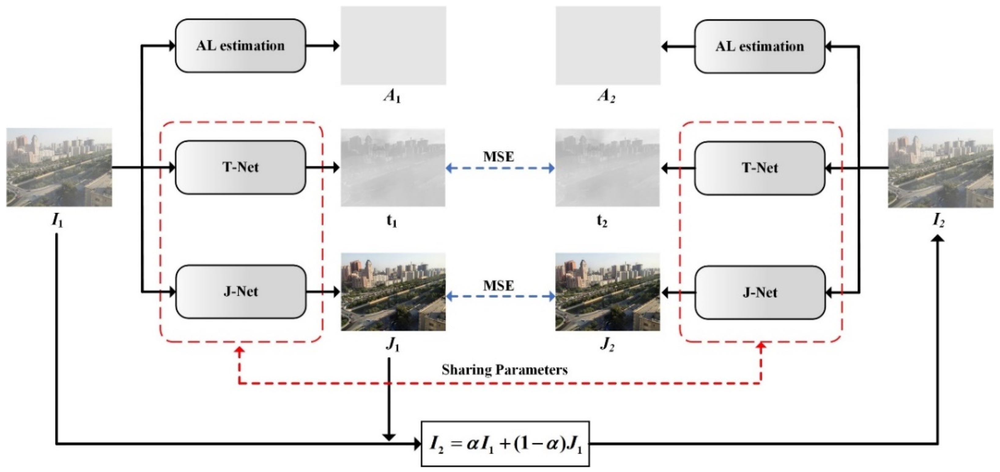
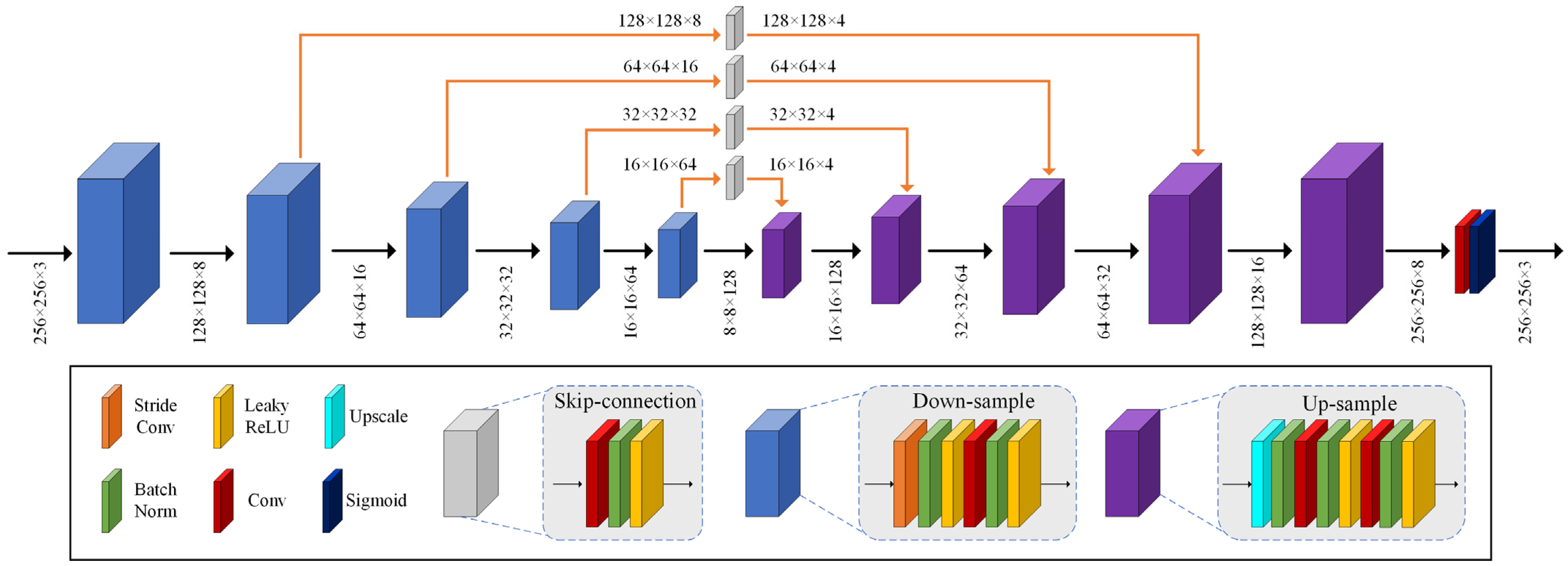
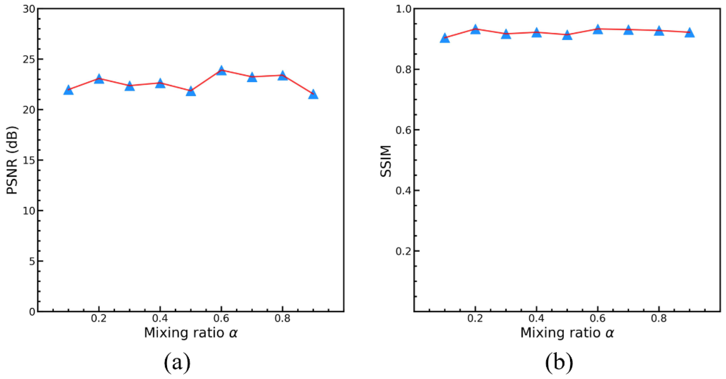
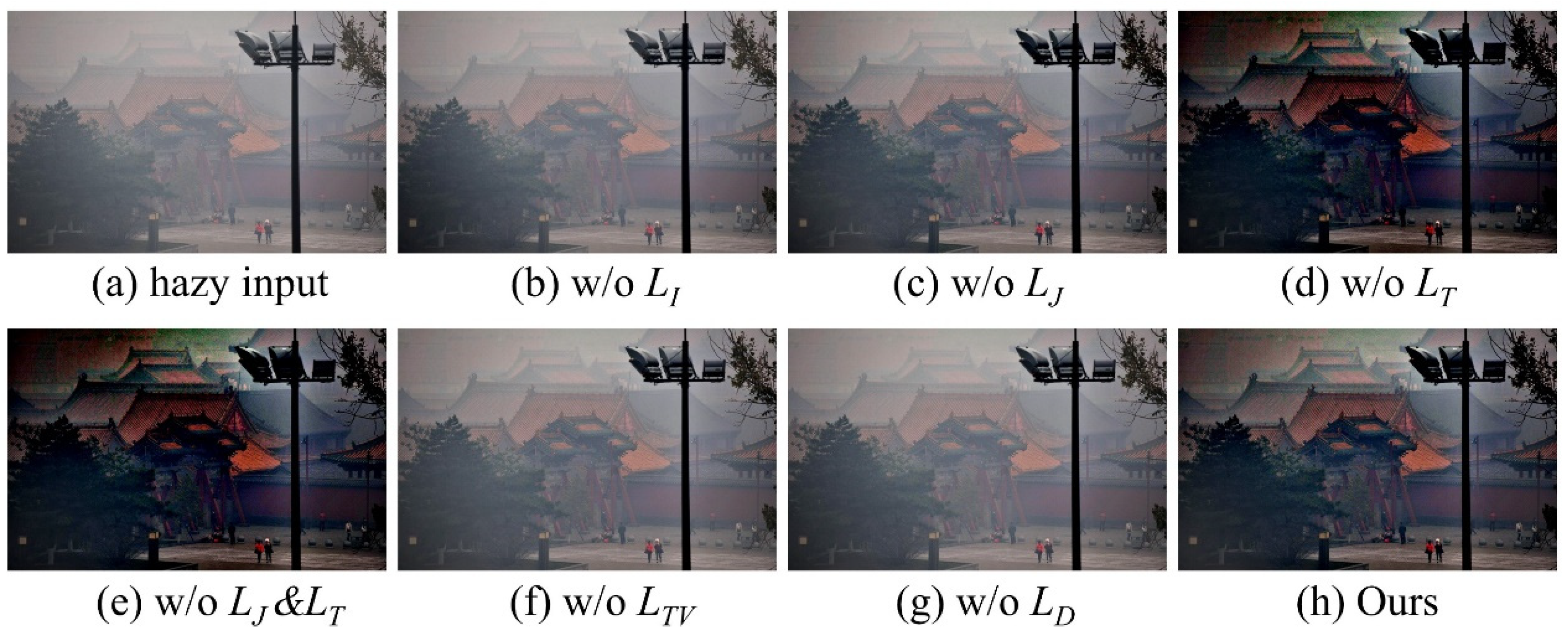
This work proposes a novel re-degradation haze imaging model for zero-shot RS image dehazing. Firstly, we design a dehazing framework consisting of three joint sub-modules: AL estimation, J-Net, and T-Net. The AL estimation module estimates the atmospheric light using a quad-tree hierarchical search algorithm. T-Net and J-Net are two neural networks to infer the transmission map and haze-free image. Thus, the dehazing framework disentangles the hazy input image into three components: the atmospheric light, the transmission map, and the recovered haze-free image. We then generate a re-degraded hazy image by mixing up the hazy input image and the recovered haze-free image. Through the proposed re-degradation haze imaging model, we theoretically demonstrate that the hazy input image and the re-degraded hazy image follow a similar haze imaging model with the same scene radiance, the same atmospheric light, and the transmission maps with known fixed relations. This finding helps us to train the dehazing network in an unsupervised fashion. Concretely, the dehazing network is optimized in a zero-shot manner to generate outputs that satisfy the relationship between the hazy input image and the re-degraded hazy image in the re-degradation haze imaging model. Therefore, given a hazy RS image, the dehazing network directly infers the haze-free image by minimizing a specific loss function. Comprehensive experiments demonstrate the effectiveness of the proposed dehazing method. To summarize, the main contributions of this paper are listed as follows:

(1) Based on layer disentanglement, we design a dehazing framework consisting of three joint sub-modules: AL estimation, J-Net, and T-Net. The AL estimation module estimates the atmospheric light. T-Net and J-Net infer the transmission map and haze-free image, respectively.

(2) We propose a novel re-degradation haze imaging model to demonstrate the relationship between the hazy input image and the re-degraded hazy image. A re-degradation loss is introduced to train the dehazing network in a zero-shot manner; that is, the dehazing network is optimized using only one hazy RS image.

(3) The proposed network recovers a haze-free image from a single RS image without large training data, hence avoiding labor-intensive data gathering and resolving the domain-shift issue brought on by synthetic datasets.

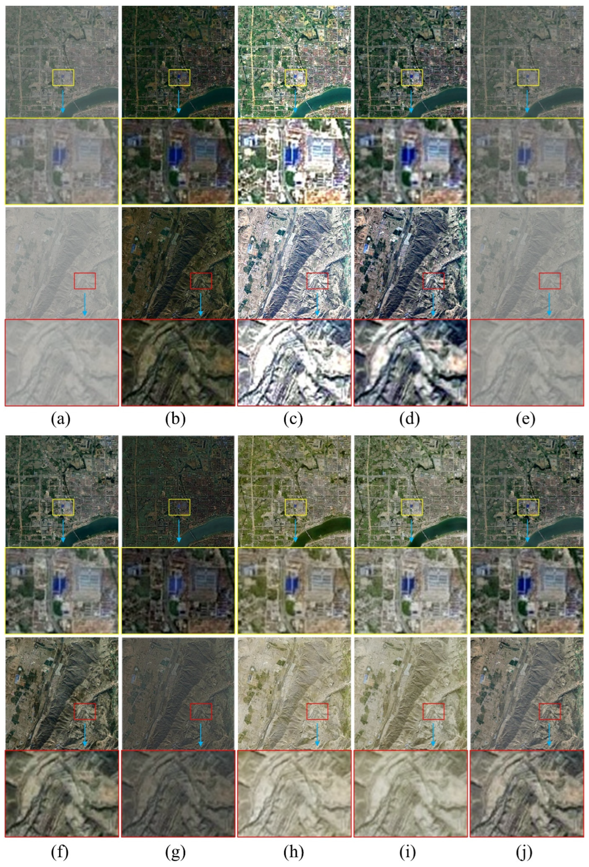
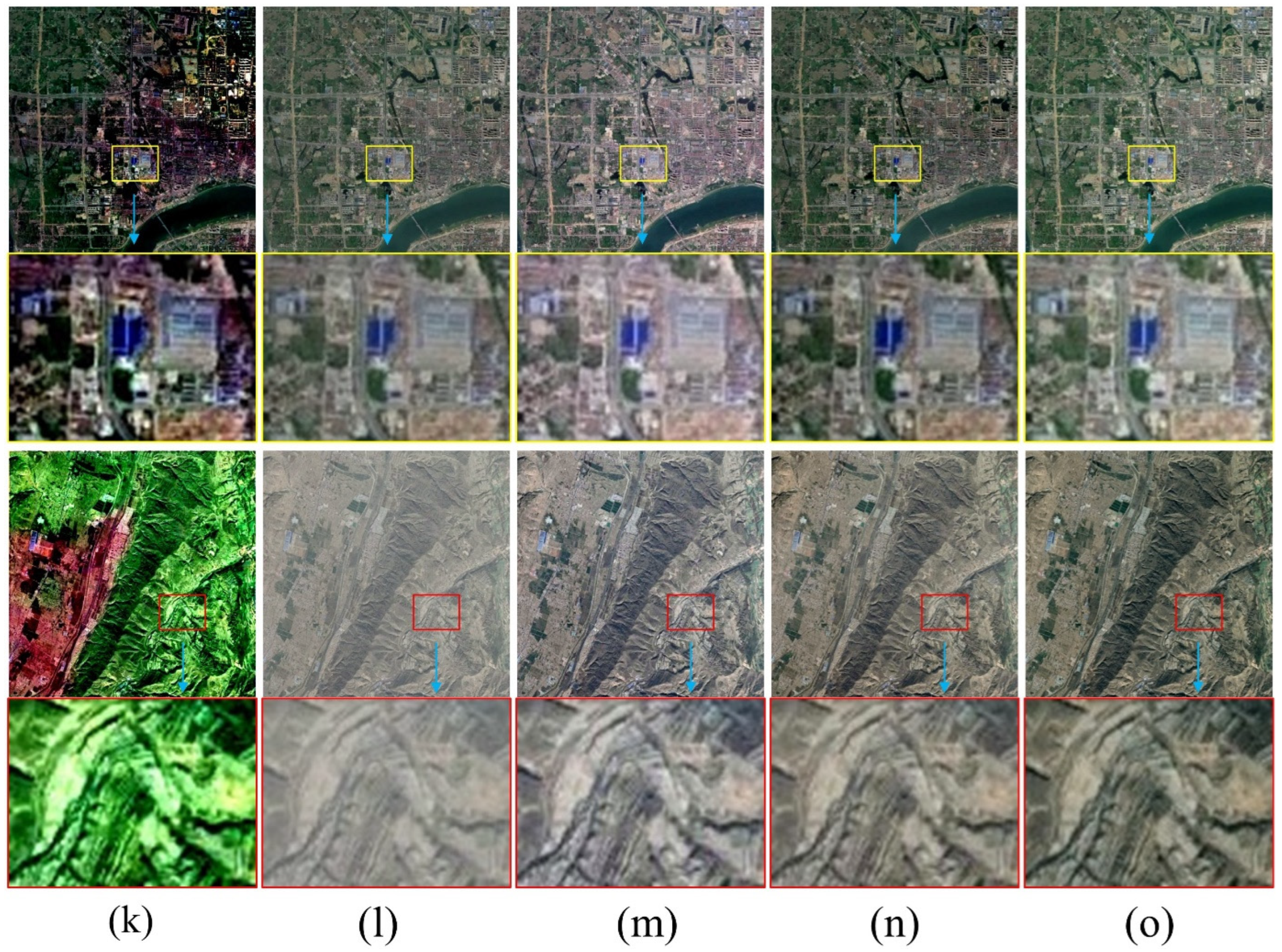
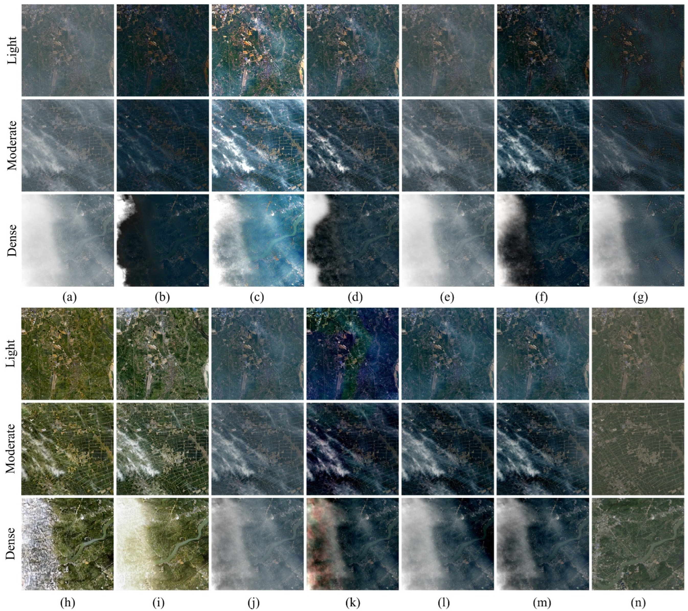
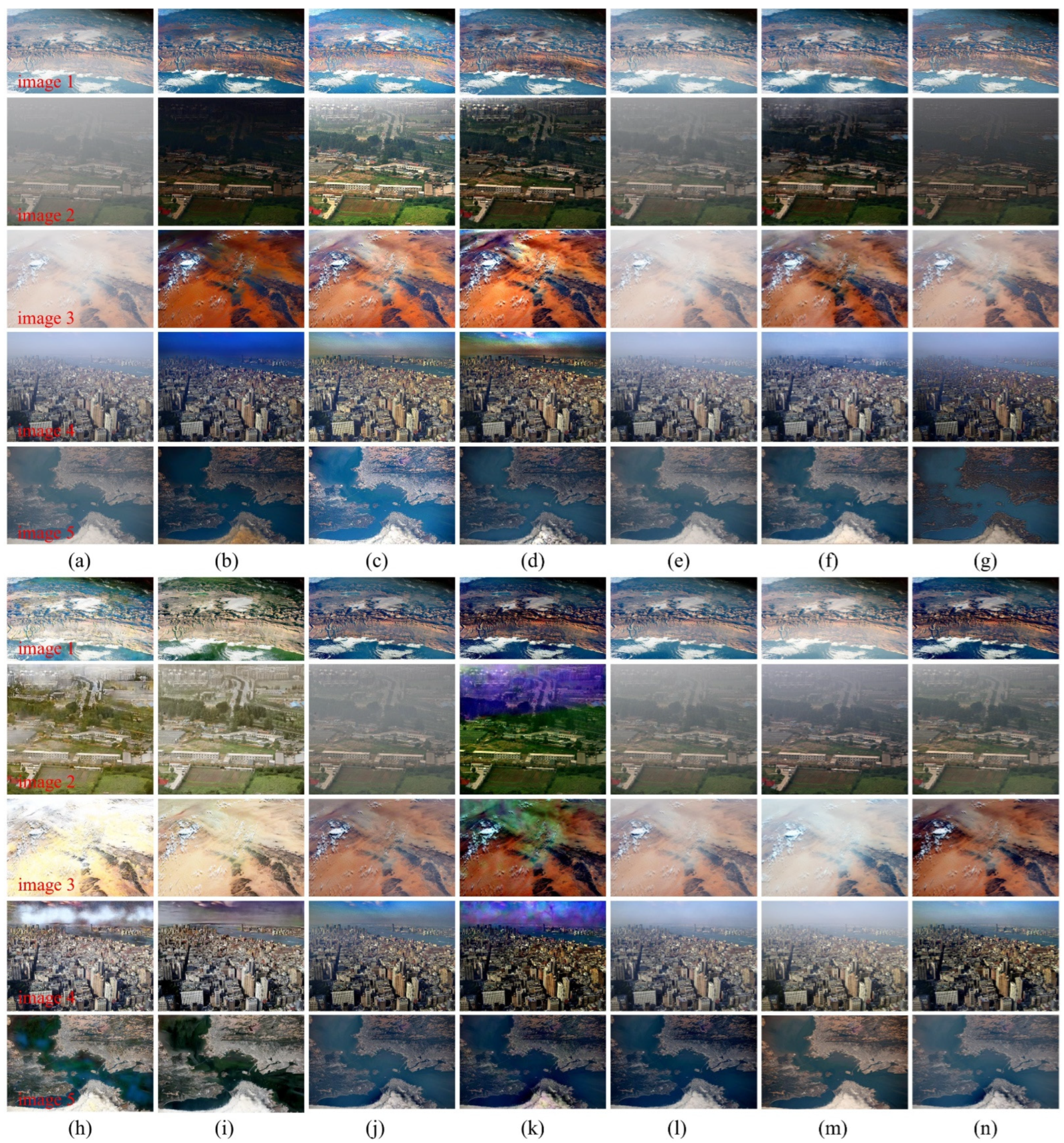
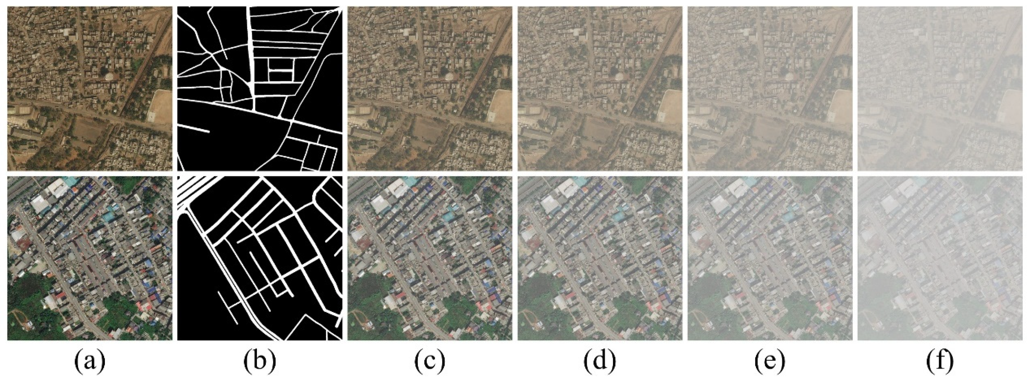
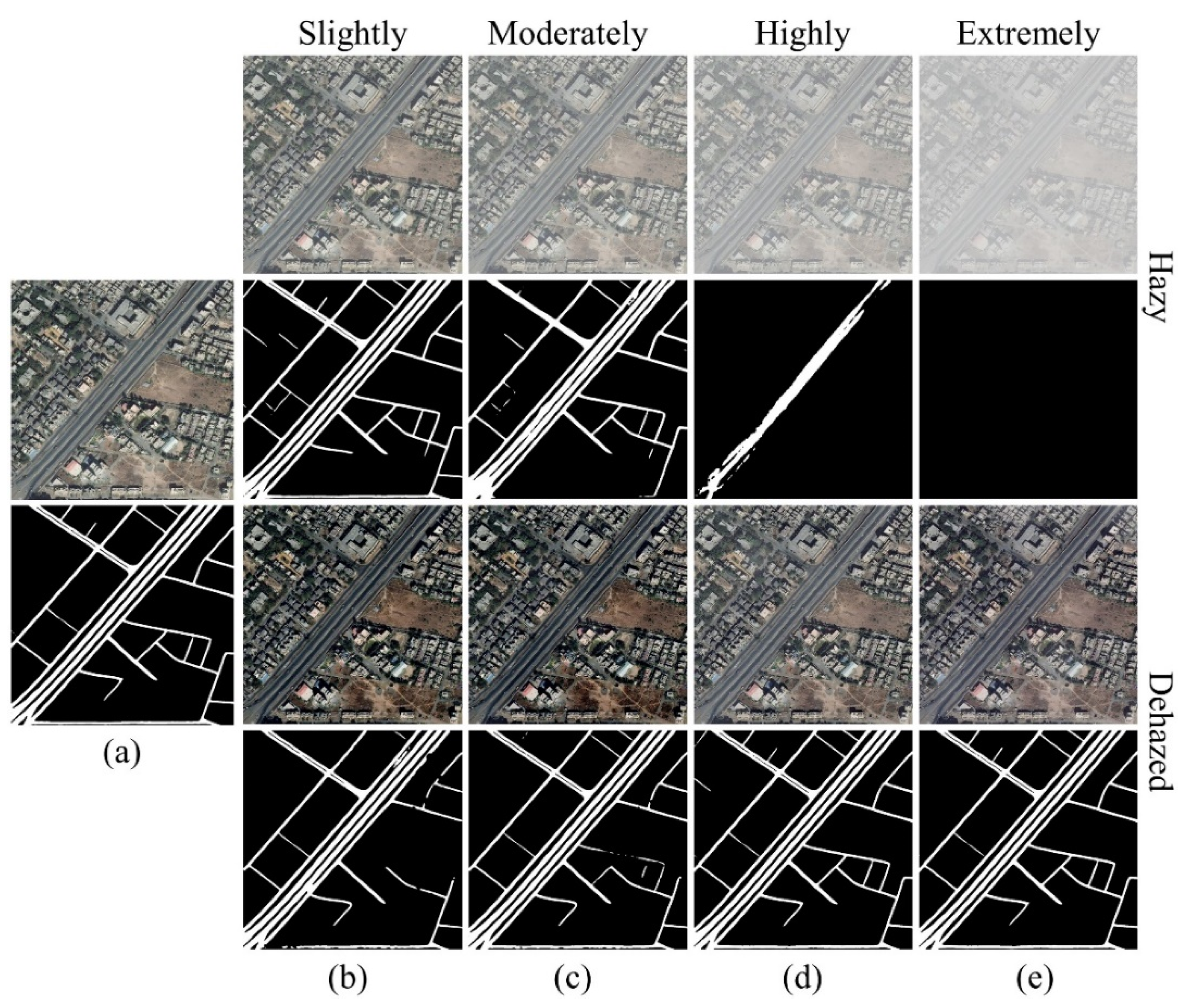
(4) In the experiments, we evaluate uniform RS hazy datasets, non-uniform RS hazy datasets, and real-world RS hazy images. Results show that our method outperforms numerous state-of-the-art (SOTA) dehazing methods in processing RS hazy images with uniform haze or slight/moderate non-uniform haze. In addition, we implement the RS image road extraction task to further demonstrate the effectiveness of our method.

2. Methodology

2.1. Re-Degradation Haze Imaging Model

According to the atmospheric scattering theory proposed by McCartney [34], the degradation of a hazy image can be formulated by the haze imaging model as follows:

$$I=Jt+A(1-t)$$

(1)

where I is the observed hazy image by the camera sensor, J is the haze-free image needing to be recovered, A is the global atmospheric light, and t is the medium transmission map. Generally, $t=e^{-\beta d}$, where $\beta$ is the scattering coefficient of the atmospheric light and d is the scene depth. The ill-posed dehazing problem is to recover J from I, which indicates that transmission map t and atmospheric light A should be estimated.

Given a hazy image I₁, according to Equation (1), we have:

$$I_1=J_1{t}_1+A_1(1-t_1)$$

(2)

where $J_1$, $t_1$, and $A_1$ are the estimated haze-free image, transmission map, and atmospheric light, respectively. Assuming the error map between the estimated haze-free image $J_1$ and the ground truth $J_{GT}$ is $\epsilon$, we obtain:

$$J_1=J_{GT}+\epsilon$$

(3)

The dehazing process can be realized by a well-designed estimator to minimize the error map $\epsilon$. Therefore, substituting $J_1$ in Equation (2) with Equation (3), we have:

$$I_1=J_{GT}{t}_1+(1-t_1)A_1+\epsilon t_1$$

(4)

We now fuse the estimated $J_1$ and original hazy image $I_1$ with a mixing ratio $\alpha \in (0,1)$ to obtain a re-degraded hazy image $I_2$ as follows:

$$I_2=\alpha I_1+(1-\alpha )J_1$$

(5)

Substituting $I_1$ in Equation (5) with Equation (2), we have:

$$I_2=J_1(\alpha t_1+1-\alpha )+\alpha (1-t_1)A_1$$

(6)

Let $t_2=\alpha t_1+1-\alpha$, then Equation (6) can be reformulated as:

$$I_2=J_1{t}_2+(1-t_2)A_1$$

(7)

Therefore, substituting $J_1$ in Equation (7) with Equation (3), we have:

$$I_2=J_{GT}{t}_2+(1-t_2)A_1+\epsilon t_2$$

(8)

One can find that if the error map $\epsilon$ is close to zero, then $\epsilon t_1=\epsilon t_2=0$. Hence, Equations (4) and (8) can be modified as follows:

$$I_1=J_{GT}{t}_1+(1-t_1)A_1$$

(9)

$$I_2=J_{GT}{t}_2+(1-t_2)A_1$$

(10)

Now, the hazy image $I_1$ and the re-degraded hazy image $I_2$ follow a similar haze imaging model with the same scene radiance $J_{GT}$ and the same global atmospheric light $A_1$. Furthermore, as the mixing ratio $\alpha$ is a preset fixed parameter, the relation of $t_1$ and $t_2$ is known, i.e., $t_2=\alpha t_1+1-\alpha$. Therefore, the re-degradation haze imaging model explained by Equations (9) and (10) can be implemented to regulate the dehazing network. Assuming a dehazing network, $F=\{F_J,F_A,F_t\}$, which estimates the haze-free image by $F_J$, atmospheric light by $F_A$, and transmission map by $F_t$, respectively. Therefore, given the hazy image $I_1$ and the re-degraded hazy image $I_2$ as inputs, the dehazing network $F$ tries to output two similar haze-free images ($F_J(I_1)$ and $F_J(I_2)$), two similar atmospheric lights ($F_A(I_1)$ and $F_A(I_2)$), and two transmission maps with fixed relation ($F_t(I_1)$ and $F_t(I_2)$).

Therefore, the minimization of the error map $\epsilon$ for the dehazing problem can be realized by minimizing the following function:

$$L=\Vert J_1-J_2\Vert +\Vert A_1-A_2\Vert +\Vert (\alpha t_1+1-\alpha )-t_2\Vert$$

(11)

where $J_i=F_J(I_i)$, $A_i=F_A(I_i)$, $t_i=F_t(I_i)$, and $i\in \{1,2\}$. $\Vert ·\Vert$ denotes L2-norm regularization. $J_1$ and $J_2$ are the recovered haze-free images from $I_1$ and $I_2$, respectively, $A_1$ and $A_2$ are the estimated atmospheric lights, and $t_1$ and $t_2$ are the estimated transmission maps. Note that the re-degraded $I_2$ is generated from $I_1$ without any other information, so the whole dehazing procedure requires only one hazy image $I_1$ as the input. Concretely, the dehazing network $F$ is optimized to generate outputs that satisfy the relationship between the hazy input image and the re-degraded hazy image in the re-degradation haze imaging model. Therefore, the dehazing network $F$ can be trained using a zero-shot training strategy.

2.2. Network Architecture

As shown in Figure 1, the overall framework of the proposed dehazing network consists of three sub-modules, i.e., the atmospheric light estimation module (AL estimation), the transmission map estimation network (T-Net), and the haze-free recovery network (J-Net). Given a hazy image $I_1$ as the input, the three sub-modules disentangle the input into $A_1$ by AL estimation module, $t_1$ by T-Net, and $J_1$ by J-Net. Based on the haze imaging model in Equation (1), we can reconstruct the hazy image ${I_1}^{\prime }$ by:

$${I_1}^{\prime }=J_1{t}_1+A_1(1-t_1)$$

(12)

Indeed, $I_1$ and ${I_1}^{\prime }$ should be cycle-consistent, which can be used to self-regulate the dehazing network. By mixing up the $I_1$ and $J_1$ with a ratio $\alpha$, we obtain a re-degraded hazy image $I_2$. The $I_2$ is then fed into the network to obtain another three outputs: $A_2$, $t_2$, and $J_2$. According to the re-degradation haze imaging model discussed in Section 2.1, $J_1$ and $J_2$ should be the same, while $t_1$ and $t_2$ have a known fixed relation. This property poses another regulation for the optimization of the proposed dehazing network. We now elaborate on the three sub-modules in detail.

AL estimation: For many dehazing frameworks using disentangle–entangle architecture, they estimate the atmospheric light (AL) by a well-designed network. For example, Li et al. [12] use a variational auto-encoder (VAE) to infer the global AL. Kar et al. [32] propose an AL network with multi-scale feature attention. Typically, a hazy image’s AL is constant in a homogenous medium, which locates in the smoothest patch with the maximum brightness. Therefore, to reduce the complexity of the whole network, we directly estimate the AL by an AL estimation module.

The proposed AL estimation module locates the AL by a quad-tree hierarchical search algorithm. Firstly, the hazy image $I$ is divided into four blocks, and the score of each block is calculated by the difference between the mean and standard deviation of the pixel values within the block. Assuming the i-th block is $I_n^i$, where $n$ is the degree of subdivision and $i\in \{1,2,3,4\}$, the score is calculated as follows:

$$S(I_n^i)=mean(I_n^i)-std(I_n^i)$$

(13)

The block with the highest score is further divided into four sub-blocks, and we repeat this process until the size of the block is under a predefined threshold. Therefore, we attempt to choose the image block as bright and hazy as possible. As shown in Figure 2, the mean value of the selected block is regarded as the estimated AL.

J-Net and T-Net: Inspired by [33,35], we take an encoder–decoder architecture with skip-connections for J-Net. As shown in Figure 3, in the encoding stage, there are five down-sampling modules to extract the image’s features in pyramid scales. We use stride convolution as the down-sampling operation. Five up-sampling modules with bilinear upscale are implemented in the decoding stage to recover the image. To reduce the information loss, skip connections using concatenate operation are employed between the corresponding layers of different levels from encoder and decoder. We use convolution with $1\times 1$ filters to reduce the dimension of feature maps to four for concatenation.

The detailed configuration of J-Net is listed in Figure 4. Given an image with the size of $256\times 256\times 3$, in the encoding stage, the image’s size is gradually down-sampled from $256\times 256$ to $8\times 8$, while the dimension is increased from 3 to 128. In the decoding stage, the image’s size is gradually up-sampled from $8\times 8$ to $256\times 256$, while the dimension decreases from 128 to 3. Note that the four skip connection layers are L3, L6, L9, and L12. The T-Net has the same network architecture as J-Net, with only one difference: the T-Net has only one output channel in the last layer (L34).

2.3. Loss Function

The following loss function in Equation (14) is formulated to train J-net and T-net jointly.

$$L=L_I+L_J+L_T+{\lambda }_1{L}_{TV}+{\lambda }_2{L}_D$$

(14)

where $L_I$ is the reconstruction loss, $L_J$ and $L_T$ are the re-degradation losses, $L_{TV}$ is the total variation loss, $L_D$ is the dark channel prior (DCP) loss, and ${\lambda }_1$ and ${\lambda }_2$ are two balancing weights. In this section, we describe each part of the loss function in detail.

Reconstruction loss. Given a hazy image $I_1$ as input, the network disentangles it into three parts: atmospheric light $A_1$ by AL estimation module, transmission map $t_1$ by T-Net, and haze-free image $J_1$ by J-Net. Therefore, we can reconstruct the hazy image ${I_1}^{\prime }$ at the top layer by the haze imaging model in Equation (1). We then minimize the subsequent reconstruction loss $L_I$ in Equation (15) by the mean square error (MSE) criterion to constrain the entire network to reconstruct the hazy image by disentanglement.

$$L_I={\Vert {I_1}^{\prime }-I_1\Vert }^2$$

(15)

Re-degradation loss. As discussed in Section 2.2, when the error map $\epsilon$ is close to zero, the two hazy input images $I_1$ and $I_2$ have similar degradation formulation. Therefore, the re-degradation loss function includes two parts $L_J$ and $L_T$ to regulate the two J-Nets and T-Nets. $L_J$ measures the dissimilarity of the recovered haze-free images $J_1$ and $J_2$, and regulates the two J-Nets to yield the same output. Thus, we compute the $L_J$ loss as follows:

$$L_J={\Vert J_1-J_2\Vert }^2$$

(16)

Similarly, as $t_2=\alpha t_1+1-\alpha$ in the re-degradation haze imaging model, the T-Nets are regulated to produce $t_2\to (\alpha t_1+1-\alpha )$ by the following loss function:

$$L_T={\Vert (\alpha t_1+1-\alpha )-t_2\Vert }^2$$

(17)

Total variation loss. An image with much noise or abrupt artifacts tends to have a higher total variation (TV) value. By reducing the total variation of an image, the unwanted noise can be removed while preserving valuable details. Therefore, in Equation (18), we use total variation loss to regulate the J-Net generating a natural haze-free image with spatial continuity and smoothness.

$$L_{TV}={\Vert {\nabla }_h{J}_1+{\nabla }_v{J}_1\Vert }^2$$

(18)

where ${\nabla }_h$ and ${\nabla }_v$ denote the horizontal and vertical differential operation matrices, respectively.

Dark channel prior loss. Dark channel prior (DCP) is one of the most significant image priors for dehazing proposed by He et al. [7]. It is based on a statistical observation that in most local patches of an outdoor haze-free image, there is at least one color channel whose pixel intensity is close to zero, as expressed below:

$$J^{Dark}=\underset{y\in \mathrm{\Omega }(x)}{\min }[\underset{c\in \{r,g,b\}}{\min }{J}^c(y)]\to 0$$

(19)

where $x$ and $y$ are pixel coordinates, $J^c$ is the c-th color channel of the haze-free image, and $\mathrm{\Omega }(x)$ is a local image patch centered at $x$. Thus, the dark channel of a haze-free image ($J^{Dark}$) tends to be zero.

Motivated by this principle, DCP loss $L_D$ is applied to constrain the dark channel of the recovered haze-free image close to zero:

$$L_D={\Vert J_1{}^{Dark}\Vert }^2$$

(20)

In this work, we adopt the look-up table scheme proposed by [36] to embed the DCP loss into the learning network.

3. Experiments and Discussions

In this section, we conduct comprehensive experiments to show the performance of the proposed method. In Section 3.1, we elaborate on the experimental settings. In Section 3.2, Section 3.3 and Section 3.4, we evaluate the dehazing performance of the proposed method using uniform RS hazy images, non-uniform RS hazy images, and real-world hazy images, respectively. In Section 3.5, we apply the proposed dehazing method to an advanced application of RS images (road extraction) for further investigation. Finally, the selection of mixing ratio $\alpha$ and the ablation study is explained in Section 3.6.

3.1. Experimental Settings

Datasets: We conduct experiments on various RS hazy datasets to obtain a comprehensive evaluation. According to the purpose of the evaluation, the testing datasets are separated into five categories: (1) RS hazy datasets with uniform haze. We choose RICE-I [28] to verify our method’s dehazing performance on uniform RS hazy images. The RICE-I includes 500 pairs of images with uniform haze or thin clouds. (2) RS hazy datasets with non-uniform haze. We use the SOTA RS-Haze dataset [26] for non-uniform dehazing evaluation. The RS-Haze is a large-scale realistic RS dehazing dataset including 54,000 RS hazy images covering light, moderate, and dense non-uniform haze. We randomly select 100 images for each haze density from the test set of RS-Haze, giving us a total of 300 hazy images for testing. (3) Real-world hazy datasets. We collected some real-world RS or aerial hazy images from Google and Flickr for real-world dehazing evaluation. The collected images cover both city scenes and natural scenes. (4) High-level vision application of RS images. To test the proposed method’s performance on advanced RS image applications, we employ the DeepGlobe road extraction dataset [37]. (5) Ablation study dataset. Since the proposed method achieves zero-shot dehazing without large-scale training datasets, we choose the tiny subset (HSTS) of RESIDE for the ablation study. In

Table 1. Datasets that are used in the experiments.

Datasets	Purpose	Brief Description
RICE-I [28]	Dehazing evaluation on RS hazy images with uniform haze.	An RS image dataset that includes 500 pairs of images with uniform haze or thin cloud.
RS-Haze [26]	Dehazing evaluation on RS hazy images with non-uniform haze.	A large-scale realistic RS dehazing dataset covering light, moderate, and dense haze density for highly non-uniform haze removal evaluation.
Real-world hazy datasets	Dehazing evaluation on real-world hazy images.	Some real-world RS or aerial hazy images collected from Google and Flickr.
DeepGlobe [37]	RS image road extraction evaluation.	A land cover classification dataset for CVPR 2018 satellite challenge.
HSTS [38]	Ablation study.	A testing subset of the RESIDE dataset, including 10 real-world hazy images and 10 pairs of synthetic images.

, we list all the datasets used in the experiments.

Training details: We train the proposed network on an NVIDIA RTX 3080 GPU using the PyTorch toolbox. The model is trained with 800 iterations for each hazy image to obtain the dehazed image. The optimization process is conducted by the ADAM optimizer, with the learning rate set to 0.001. For the balancing weights of loss function in Equation (14), we set ${\lambda }_1=5\times {10}^{-5}$ and ${\lambda }_2={10}^{-6}$. For the mixing ratio $\alpha$ in Equation (5), we set α = 0.8, with the impact of $\alpha$ on the dehazing performance discussed in Section 3.6.1.

Baselines: As shown in Table 2, we evaluate the performance against 13 SOTA dehazing methods, including four traditional dehazing methods, five supervised learning-based methods, and four zero-shot dehazing methods. To be specific, the traditional dehazing methods contain DCP, MOF, CAP, and BCDP. The supervised-learning-based methods are FFA, EMRA, LDN, AESUN, and TBNN, where AESUN and TBNN are non-uniform dehazing methods. The zero-shot dehazing methods include DDIP, ZID, YOLY, and ZIR. To better compare the generalizability of different methods, we use official pretrained models for all the supervised-learning-based methods.

Table 2. Thirteen dehazing methods for comparison are divided into three categories: traditional dehazing methods, supervised-learning-based dehazing methods, and zero-shot dehazing methods.

Category	Method	Short Explanation
Traditional	DCP [7]	Dark channel prior
	MOF [5]	Multi-scale optimal fusion
	CAP [4]	Color attenuation prior
	BCDP [6]	Bounded channel difference prior
Supervised	FFA [10]	Feature fusion attention network
	EMRA [39]	Ensemble multi-scale residual attention network
	LDN [40]	Lightweight CNN dehazing network
	AESUN [35]	Attention enhanced serial Unet++ network
	TBNN [41]	Two-branch neural network via ensemble learning
Zero-shot	DDIP [30]	Coupled deep image prior
	ZID [31]	Zero-shot dehazing
	YOLY [12]	You only look yourself
	ZIR [32]	Zero-shot single image restoration

Table 2. Thirteen dehazing methods for comparison are divided into three categories: traditional dehazing methods, supervised-learning-based dehazing methods, and zero-shot dehazing methods.

Category	Method	Short Explanation
Traditional	DCP [7]	Dark channel prior
	MOF [5]	Multi-scale optimal fusion
	CAP [4]	Color attenuation prior
	BCDP [6]	Bounded channel difference prior
Supervised	FFA [10]	Feature fusion attention network
	EMRA [39]	Ensemble multi-scale residual attention network
	LDN [40]	Lightweight CNN dehazing network
	AESUN [35]	Attention enhanced serial Unet++ network
	TBNN [41]	Two-branch neural network via ensemble learning
Zero-shot	DDIP [30]	Coupled deep image prior
	ZID [31]	Zero-shot dehazing
	YOLY [12]	You only look yourself
	ZIR [32]	Zero-shot single image restoration

3.2. Evaluation of RS Images with Uniform Haze

To evaluate the RS image dehazing performance on uniform hazy images, we compare our method with SOTA dehazing methods on RICE-I [28]. We randomly select two images covering city scenes and mountain scenes from the RICE-I test set as inputs. The recovered haze-free images by various dehazing methods are shown in Figure 5. Specifically, Figure 5a is the hazy input image, Figure 5b–n are the recovered haze-free images by various dehazing methods, and Figure 5o is the reference ground truth. A close-up indicated by the blue arrow is shown below the corresponding image for better comparison.

As shown in Figure 5, it can be seen that ZID obtains the worst results with severe color distortion, whereas the recovered images by FFA and YOLY have plenty of haze. Although DCP and LDN can remove haze properly, the dehazed images tend to have a darker color than the ground truth. For the results by MOF and BCDP, obvious over-enhancement can be found in the close-up of the red rectangle in Figure 5c,d. As shown in Figure 5h,i, the dehazed images by AESUN and TBNN show slight color distortion compared with the reference image in Figure 5o. From Figure 5f,j,n, the recovered haze-free images by EMRA, DDIP, and our method are visually closer to the ground truth. Therefore, from the qualitative comparison, our proposed method outperforms most of the SOTA dehazing methods in processing uniform RS hazy images.

In addition, we quantitatively analyze the performance of different methods by evaluating three IQA indexes (PSNR, SSIM, and CIEDE2000) on the RICE-I dataset. The CIEDE2000 [42] measures the color difference between the dehazed image and the ground truth, with a lower CIEDE2000 value indicating better color consistency. The quantitative evaluation results for RICE-I are shown in

Table 3. Quantitative evaluation results for the RS uniform hazy dataset (RICE-I). The best value of the specific metric for each category is in boldface.

Category	Method	PSNR	SSIM	CIEDE2000
Traditional	DCP	11.6	0.58	7.77
	MOF	17.54	0.53	16.32
	CAP	24.85	0.87	9.39
	BCDP	21.2	0.65	18.64
Supervised	FFA	25.81	0.82	7.98
	EMRA	16.6	0.82	4.89
	LDN	15.46	0.76	5.26
	AESUN	18.58	0.67	4.62
	TBNN	19.07	0.73	4.04
Zero-shot	DDIP	24.65	0.87	10.69
	ZID	19.23	0.53	26.13
	YOLY	24.34	0.85	11.31
	Ours	24.76	0.88	10.23

, where the testing methods are divided into three categories: traditional dehazing methods, supervised-learning-based methods, and zero-shot dehazing methods. We mark the best value of the specific metric for each category in boldface. From Table 3, it can be seen that, for traditional dehazing methods, DCP has the best CIEDE2000 value and CAP has the best PSNR and SSIM values. For supervised-learning-based methods, FFA outperforms the other methods in PSNR value by a large margin. Both FFA and EMRA have the best SSIM value, while TBNN obtains the best CIEDE2000 value. In the zero-shot dehazing category, our method obtains the best results for all three IQA indexes. In addition, our method has better PSNR and SSIM values than most dehazing methods in the traditional and supervised-learning categories. Moreover, Figure 5 and Table 3 reveal that the supervised-learning-based methods trained on synthetic ground hazy images achieve comparatively unsatisfactory performance on the RS uniform hazy dataset (RICE-I). Thus, the zero-shot dehazing methods show better generalizability than the supervised-learning-based methods.

3.3. Evaluations of RS Images with Non-Uniform Haze

RS-Haze [26] is a large-scale realistic RS dehazing dataset for non-uniform dehazing task evaluation. According to the haze density, the images in RS-Haze can be divided into lightly hazy, moderately hazy, and densely hazy. We randomly select 100 images from the test set of RS-Haze for each haze density, giving us a total of 300 hazy images for testing. For comparison, both qualitative and quantitative evaluations are conducted.

The dehazing results by various SOTA methods on the RS-Haze dataset are shown in Figure 6, where Figure 6a shows the hazy input images with light haze, moderate haze, and dense haze. Figure 6b–m are the dehazed results by various methods and our method, while Figure 6n is the reference ground truth. AESUN and TBNN, as non-uniform dehazing methods, obtain the best visual results for light and moderate hazy images. As shown in Figure 6c,k, MOF and ZID have the worst non-uniform haze removal capability and suffer from severe color distortion. DCP, EMRA, and LDN can remove light and most moderate non-uniform haze, but darker color and detailed information loss are the main problems. According to the dehazed results by FFA and DDIP, there is plenty of remaining haze, especially in moderately hazy images (see Figure 6e,j). BCDP, YOLY, and our method seem to have comparable dehazing performance for light and moderate haze removal. For dense non-uniform hazy images, all the dehazing methods fail to remove the haze properly, even the non-uniform dehazing methods (AESUN and TBNN). In conclusion, when non-uniform haze is present in the hazy images, most dehazing methods produce worse dehazing outcomes than when processing uniform hazy images, with the exception of the non-uniform dehazing approaches (AESUN and TBNN). However, our proposed method still obtains competitive results when processing light and moderately hazy images.

The quantitative evaluation results on RS-Haze are shown in

Table 4. Quantitative evaluation results on the RS non-uniform hazy dataset (RS-Haze). The best value of the specific metric for each category is in boldface.

Category		Traditional				Supervised					Zero-Shot
Density	Metrics	DCP	MOF	CAP	BCDP	FFA	EMRA	LDN	AESUN	TBNN	DDIP	ZID	YOLY	Ours
Light	PSNR	15.88	12.42	21.23	19.85	20.96	17.14	16.77	19.48	20.13	21.25	15.22	19.84	21.48
	SSIM	0.22	0.27	0.39	0.43	0.45	0.29	0.33	0.65	0.73	0.43	0.25	0.39	0.49
	CIEDE	6.48	7.96	4.24	4.71	4.07	5.79	5.75	3.94	3.09	4.19	6.79	4.70	4.26
Moderate	PSNR	15.51	10.28	16.97	17.22	14.67	16.48	17.53	16.48	15.57	17.65	15.40	15.83	17.77
	SSIM	0.13	0.13	0.25	0.26	0.36	0.23	0.30	0.62	0.68	0.33	0.25	0.28	0.38
	CIEDE	6.71	9.81	5.52	5.82	6.08	6.09	5.32	4.86	4.56	5.15	6.68	5.97	5.15
Dense	PSNR	14.34	9.01	13.64	15.27	9.95	14.30	14.17	11.00	10.52	14.48	13.88	12.21	14.38
	SSIM	0.19	0.10	0.22	0.21	0.32	0.26	0.33	0.48	0.56	0.30	0.19	0.27	0.28
	CIEDE	6.72	10.52	6.71	6.22	9.28	6.46	6.19	7.57	7.83	6.12	7.13	7.58	6.12
Average	PSNR	15.24	10.57	17.28	17.45	15.19	15.97	16.16	15.65	15.41	17.79	14.83	15.96	17.88
	SSIM	0.18	0.17	0.29	0.30	0.38	0.26	0.32	0.58	0.66	0.36	0.23	0.31	0.39
	CIEDE	6.64	9.43	5.49	5.58	6.48	6.11	5.75	5.45	5.16	5.15	6.87	6.08	5.18

. We calculate PSNR, SSIM, and CIEDE2000 indexes for different haze densities, with the average results compared. In Table 4, the best value of the specific metric for each category is marked in boldface. For traditional dehazing methods, BCDP obtains the best results followed by CAP. For supervised-learning-based methods, AESUN and TBNN outperform other methods in the SSIM index by a large margin, while TBNN has the best SSIM and CIEDE2000 values on average. In the zero-shot dehazing category, our method obtains the best results in both light and moderate haze density, while DDIP has the best results in processing dense hazy images. On average, our method outperforms the other zero-shot dehazing methods with the best IQA metrics values. Moreover, even compared with the dehazing methods in traditional and supervised categories, our method shows better results for PSNR and CIEDE2000 values.

3.4. Evaluations of Real-World RS Hazy Images

In order to analyze the real-world dehazing performance, we collected real-world RS and aerial hazy images from Google and Flickr for testing. As shown in Figure 7, the testing images are labeled ‘image 1’ to ‘image 5’, where all five images have uniform haze except for ‘image 3’ which has a slight non-uniform haze. Figure 7a is the input hazy images, Figure 7b–m are the dehazed results by various SOTA dehazing results, and Figure 7n is our dehazed results.

As shown in Figure 7k, ZID presents the worst results with severe color distortion, especially in the sky region of ‘image 2’ and ‘image 4’. According to ‘image 2’, ‘image 4’, and ‘image 5’ in Figure 7b,g, the dehazed images by DCP and LDN result in dark color and detailed information lost. FFA, YOLY, and ZIR cannot remove haze thoroughly, especially the non-uniform haze in ‘image 3’. AESUN and TBNN, as trained on non-uniform hazy datasets, suffer from severe domain-shift issues in processing real-world RS hazy images. Thus, they obtain poor results with color distortion and undesired artifacts (see ‘image 2’ and ‘image 4’ in Figure 7h,i). Although BCDP achieves good haze removal capability, over-enhancement can be found in ‘image 4’ of Figure 7d, while slight color shift occurs in ‘image 3’ of Figure 7d. MOF and EMRA show good haze removal capability, but there is slight color distortion in ‘image 1’ and ‘image 5’ of Figure 7c, while ‘image 2’ of Figure 7f loses the shadow details. DDIP and our method obtain visually better results than the other methods, but there is more residual haze in Figure 7j than in Figure 7n. Therefore, compared with the SOTA dehazing methods, our proposed method shows better dehazing results on processing RS hazy images with uniform haze or slight non-uniform haze. In addition, the results also show the better generalizability of our method due to the zero-shot learning manner.

3.5. Application of Dehazing on RS Image Road Extraction

To further investigate the dehazing algorithms for improving the performance of advanced RS image applications, we compare the results of RS image road extraction by using different image dehazing methods as prepossessing. To this end, we select the DeepGlobe road extraction dataset [37] to generate the testing data. Firstly, we randomly select 30 haze-free images from DeepGlobe. Note that each image has a corresponding ground truth road mask for evaluation. For each haze-free image, we then generate four hazy images of different densities by the haze imaging model defined in Equation (1). Finally, we obtain 120 hazy images in total for testing. Samples of the generated hazy RS image from the DeepGlobe dataset are shown in Figure 8, where Figure 8a is the original haze-free image, Figure 8b is the ground truth road mask, and Figure 8c–f are the four generated hazy images of different haze densities defined as slightly hazy, moderately hazy, highly hazy, and extremely hazy, respectively.

Given the generated hazy images as inputs, we obtain the recovered haze-free images by different dehazing methods. We then use a pre-trained D-LinkNet [43] to extract road masks from the dehazed images. As shown in Figure 9, the D-LinkNet can extract the road when the haze density is slight. However, as the haze density increases, the D-LinkNet can hardly obtain good results using the hazy images and fails to extract any road tracks under an extremely hazy situation. As shown in the third row of Figure 9b–e, our method removes the haze effectively and recovers the full road details. Using the dehazed images obtained by our method, the D-LinkNet can accurately extract the road, even for extremely hazy images. Therefore, our proposed dehazing method can greatly boost the road extraction accuracy of the D-LinkNet.

To quantitatively compare with the other dehazing methods, we select four standard road extraction evaluation metrics [44] for comparison, i.e., Precision, Recall, IoU, and F1-Score. The representations of the four metrics are as follows:

$$Precision=\frac{TP}{TP+FP},Recall=\frac{TP}{TP+FN},IoU=\frac{TP}{TP+FN+FP},$$

(21)

$$F1-Score=\frac{2\ast \mathrm{Pr}ecision\ast Recall}{Precision+Recall}$$

(22)

where TP, FN, and FP are the true positive, false negative, and false positive values, respectively. We first use the dehazed images from various dehazing methods to extract the road mask by D-LinkNet. We then calculate the four metrics using the ground truth road mask and the extracted road mask. Finally, the average value of the testing images is compared.

As shown in

Table 5. Quantitative comparisons of D-LinkNet road extraction accuracy using clear images and hazy images.

Input	Precision	Recall	IoU	F1-Score
Clear	0.935	0.914	0.859	0.924
Hazy	0.387	0.384	0.239	0.385

, the results of D-LinkNet road extraction using clear images are much better than those using hazy images, indicating that haze dramatically reduces the road detection accuracy of the D-LinkNet. Quantitative comparisons of D-LinkNet road extraction accuracy using the dehazed images of different dehazing methods are shown in

Table 6. Quantitative comparisons of D-LinkNet road extraction accuracy using the dehazed images of different dehazing methods. The best value of the specific metric for each category is in boldface.

Category	Method	Precision	Recall	IoU	F1-Score
Traditional	DCP	0.895	0.884	0.801	0.890
	MOF	0.640	0.657	0.480	0.648
	CAP	0.689	0.683	0.522	0.686
	BCDP	0.772	0.791	0.641	0.781
Supervised	FFA-Net	0.796	0.779	0.649	0.787
	EMRA	0.890	0.880	0.793	0.885
	LDN	0.767	0.764	0.620	0.766
	AESUN	0.547	0.568	0.386	0.557
	TBNN	0.653	0.665	0.491	0.659
Zero-shot	DDIP	0.790	0.786	0.651	0.788
	ZID	0.647	0.671	0.491	0.659
	YOLY	0.652	0.653	0.484	0.652
	Ours	0.805	0.813	0.679	0.809

. For traditional dehazing methods and supervised-learning-based methods, DCP and EMRA obtain the best results, respectively, while for zero-shot dehazing methods, our method has the best results. Although DCP and EMRA have better results than ours in Table 6, our method outperforms many SOTA traditional dehazing methods (CAP, MOF, and BCDP) and supervised-learning-based methods (FFA, LDN, AESUN, and TBNN). Therefore, our proposed dehazing method has more promising results than the other methods in improving the performance of the high-vision RS image task.

3.6. Discussions

3.6.1. Selection of the Mixing Ratio

As discussed in Section 2.1, the value of the mixing ratio ($\alpha$) is between 0 and 1. In order to investigate the impact of $\alpha$ on the performance of the re-degradation haze imaging model, we vary $\alpha$ from 0.1 to 0.9 at a step of 0.1, and calculate the average PSNR and SSIM on the HSTS dataset [38] for comparison. Testing results with different mixing ratios ($\alpha$) on the HSTS dataset are shown in Figure 10. The values of PSNR and SSIM with different $\alpha$ are slightly different. The standard deviation of PSNR and SSIM values are 0.747 dB and 0.009, respectively. Therefore, we observe that the dehazing performance is not sensitive to the selection of $\alpha$.

3.6.2. Ablation Study on the Loss Function

To verify the effectiveness of the loss function, we compare the dehazing results on the HSTS dataset by removing parts of the loss function, i.e., $L_I$, $L_J$, $L_T$, $L_{TV}$, and $L_D$. A qualitative ablation study for the loss function on a real-world hazy image dehazing is shown in Figure 11. It can be seen that the dehazed result by our method is better than the results of removing any part of the loss function. In addition, from the results of the quantitative ablation study for the loss function in

Table 7. Quantitative ablation study for the loss function on the HSTS dataset [38]. ‘w/o’ is the abbreviation of ‘without’. The best value of the specific metric is in boldface.

Metrics	w/o LI	w/o LJ	w/o LT	w/o LJ & LT	w/o LTV	w/o LD	Ours
PSNR	21.236	22.954	19.517	19.284	23.570	22.820	23.917
SSIM	0.895	0.926	0.871	0.869	0.925	0.931	0.933

, our method obtains the best PSNR and SSIM on the HSTS dataset, which further demonstrates the effectiveness of our loss function.

4. Conclusions

In this paper, we propose a re-degradation haze imaging model for zero-shot RS image dehazing. Motivated by layer disentanglement, we design a dehazing framework consisting of three sub-modules: AL estimation for atmospheric light estimation, T-Net for transmission map estimation, and J-Net for haze-free image recovery. A re-degraded hazy image is obtained by mixing up the hazy input image and the inferred haze-free image. We propose a re-degradation haze imaging model to theoretically demonstrate that the hazy input image and the re-degraded hazy image follow a similar haze imaging model. This finding helps us to design a re-degradation loss to train the dehazing network in a zero-shot manner; that is, the dehazing network is optimized using only one hazy RS image. We conduct qualitative and quantitative evaluations on both uniform and non-uniform RS hazy image datasets to show the effectiveness and promising performance of the proposed method. The results show that, in processing uniform and slight/moderate non-uniform RS hazy images, our method outperforms all zero-shot dehazing methods, and obtains better results than many traditional dehazing methods and supervised-learning-based methods. A benefit from the zero-shot learning manner is that our method shows better generalizability than the supervised-learning-based methods in the real-world image dehazing task. In addition, the evaluation on a high-level vision task (road extraction) also proves the effectiveness of our method. However, for the hazy images with dense non-uniform haze, our method fails to recover the haze-free image, which remains a task for our future research.

References

1. Chen, T.; Liu, M.; Gao, T.; Cheng, P.; Mei, S.; Li, Y. A Fusion-Based Defogging Algorithm. Remote Sens. 2022, 14, 425. [Google Scholar] [CrossRef]
2. Zhu, Z.; Luo, Y.; Qi, G.; Meng, J.; Li, Y.; Mazur, N. Remote sensing image defogging networks based on dual self-attention boost residual octave convolution. Remote Sens. 2021, 13, 3104. [Google Scholar] [CrossRef]
3. Liu, J.; Wang, S.; Wang, X.; Ju, M.; Zhang, D. A review of remote sensing image dehazing. Sensors 2021, 21, 3926. [Google Scholar] [CrossRef] [PubMed]
4. Zhu, Q.; Mai, J.; Shao, L. A fast single image haze removal algorithm using color attenuation prior. IEEE Trans. Image Process. 2015, 24, 3522–3533. [Google Scholar]
5. Zhao, D.; Xu, L.; Yan, Y.; Chen, J.; Duan, L.-Y. Multi-scale optimal fusion model for single image dehazing. Signal Process. Image Commun. 2019, 74, 253–265. [Google Scholar] [CrossRef]
6. Zhao, X. Single Image Dehazing Using Bounded Channel Difference Prior. In Proceedings of the IEEE/CVF Conference on Computer Vision and Pattern Recognition, Nashville, TN, USA, 19–25 June 2021; pp. 727–735. [Google Scholar]
7. He, K.; Sun, J.; Tang, X. Single image haze removal using dark channel prior. IEEE Trans. Pattern Anal. Mach. Intell. 2010, 33, 2341–2353. [Google Scholar]
8. Li, B.; Peng, X.; Wang, Z.; Xu, J.; Feng, D. Aod-net: All-in-one dehazing network. In Proceedings of the IEEE International Conference on Computer Vision, Venice, Italy, 22–29 October 2017; pp. 4770–4778. [Google Scholar]
9. Li, H.; Li, J.; Zhao, D.; Xu, L. DehazeFlow: Multi-scale Conditional Flow Network for Single Image Dehazing. In Proceedings of the 29th ACM International Conference on Multimedia, Virtual, 20–24 October 2021; pp. 2577–2585. [Google Scholar]
10. Qin, X.; Wang, Z.; Bai, Y.; Xie, X.; Jia, H. FFA-Net: Feature fusion attention network for single image dehazing. In Proceedings of the AAAI Conference on Artificial Intelligence, New York, NY, USA, 7–12 February 2020; Volume 34, pp. 11908–11915. [Google Scholar]
11. Liu, X.; Ma, Y.; Shi, Z.; Chen, J. Griddehazenet: Attention-based multi-scale network for image dehazing. In Proceedings of the IEEE/CVF International Conference on Computer Vision, Seoul, Korea, 27 October–2 November 2019; pp. 7314–7323. [Google Scholar]
12. Li, B.; Gou, Y.; Gu, S.; Liu, J.Z.; Zhou, J.T.; Peng, X. You only look yourself: Unsupervised and untrained single image dehazing neural network. Int. J. Comput. Vis. 2021, 129, 1754–1767. [Google Scholar] [CrossRef]
13. Kim, T.K.; Paik, J.K.; Kang, B.S. Contrast enhancement system using spatially adaptive histogram equalization with temporal filtering. IEEE Trans. Consum. Electron. 1998, 44, 82–87. [Google Scholar]
14. Xu, H.; Zhai, G.; Wu, X.; Yang, X. Generalized equalization model for image enhancement. IEEE Trans. Multimed. 2013, 16, 68–82. [Google Scholar] [CrossRef]
15. Dippel, S.; Stahl, M.; Wiemker, R.; Blaffert, T. Multiscale contrast enhancement for radiographies: Laplacian pyramid versus fast wavelet transform. IEEE Trans. Med. Imaging 2002, 21, 343–353. [Google Scholar] [CrossRef]
16. Cooper, T.J.; Baqai, F.A. Analysis and extensions of the Frankle-McCann Retinex algorithm. J. Electron. Imaging 2004, 13, 85–92. [Google Scholar] [CrossRef]
17. Seow, M.-J.; Asari, V.K. Ratio rule and homomorphic filter for enhancement of digital colour image. Neurocomputing 2006, 69, 954–958. [Google Scholar] [CrossRef]
18. Kim, J.-H.; Jang, W.-D.; Sim, J.-Y.; Kim, C.-S. Optimized contrast enhancement for real-time image and video dehazing. J. Vis. Commun. Image Represent. 2013, 24, 410–425. [Google Scholar] [CrossRef]
19. Wang, W.; Yuan, X.; Wu, X.; Liu, Y. Fast image dehazing method based on linear transformation. IEEE Trans. Multimed. 2017, 19, 1142–1155. [Google Scholar] [CrossRef]
20. Wang, J.; Lu, K.; Xue, J.; He, N.; Shao, L. Single image dehazing based on the physical model and MSRCR algorithm. IEEE Trans. Circuits Syst. Video Technol. 2017, 28, 2190–2199. [Google Scholar] [CrossRef]
21. Bie, Y.; Yang, S.; Huang, Y. Single Remote Sensing Image Dehazing using Gaussian and Physics-Guided Process. IEEE Geosci. Remote Sens. Lett. 2022, 19, 1–5. [Google Scholar] [CrossRef]
22. Chen, W.-T.; Fang, H.-Y.; Ding, J.-J.; Kuo, S.-Y. PMHLD: Patch map-based hybrid learning DehazeNet for single image haze removal. IEEE Trans. Image Process. 2020, 29, 6773–6788. [Google Scholar] [CrossRef]
23. Chen, X.; Huang, Y. Memory-Oriented Unpaired Learning for Single Remote Sensing Image Dehazing. IEEE Geosci. Remote Sens. Lett. 2022, 19, 1–5. [Google Scholar] [CrossRef]
24. Jiang, B.; Chen, G.; Wang, J.; Ma, H.; Wang, L.; Wang, Y.; Chen, X. Deep Dehazing Network for Remote Sensing Image with Non-Uniform Haze. Remote Sens. 2021, 13, 4443. [Google Scholar] [CrossRef]
25. Engin, D.; Genç, A.; Kemal Ekenel, H. Cycle-dehaze: Enhanced cyclegan for single image dehazing. In Proceedings of the IEEE Conference on Computer Vision and Pattern Recognition Workshops, Salt Lake City, UT, USA, 18–22 June 2018; pp. 825–833. [Google Scholar]
26. Song, Y.; He, Z.; Qian, H.; Du, X. Vision Transformers for Single Image Dehazing. arXiv 2022, arXiv:2204.03883. [Google Scholar]
27. Dong, P.; Wang, B. TransRA: Transformer and residual attention fusion for single remote sensing image dehazing. Multidimens. Syst. Signal Process. 2022, 33, 1119–1138. [Google Scholar] [CrossRef]
28. Lin, D.; Xu, G.; Wang, X.; Wang, Y.; Sun, X.; Fu, K. A remote sensing image dataset for cloud removal. arXiv 2019, arXiv:1901.00600. [Google Scholar]
29. Huang, B.; Zhi, L.; Yang, C.; Sun, F.; Song, Y. Single satellite optical imagery dehazing using SAR image prior based on conditional generative adversarial networks. In Proceedings of the IEEE/CVF Winter Conference on Applications of Computer Vision, Snowmass, CO, USA, 1–5 March 2020; pp. 1806–1813. [Google Scholar]
30. Gandelsman, Y.; Shocher, A.; Irani, M. “double-dip”: Unsupervised image decomposition via coupled deep-image-priors. In Proceedings of the IEEE/CVF Conference on Computer Vision and Pattern Recognition, Long Beach, CA, USA, 15–20 June 2019; pp. 11026–11035. [Google Scholar]
31. Li, B.; Gou, Y.; Liu, J.Z.; Zhu, H.; Zhou, J.T.; Peng, X. Zero-shot image dehazing. IEEE Trans. Image Process. 2020, 29, 8457–8466. [Google Scholar] [CrossRef] [PubMed]
32. Kar, A.; Dhara, S.K.; Sen, D.; Biswas, P.K. Zero-Shot Single Image Restoration through Controlled Perturbation of Koschmieder’s Model. In Proceedings of the IEEE/CVF Conference on Computer Vision and Pattern Recognition, Nashville, TN, USA, 20–25 June 2021; pp. 16205–16215. [Google Scholar]
33. Ulyanov, D.; Vedaldi, A.; Lempitsky, V. Deep image prior. In Proceedings of the IEEE Conference on Computer Vision and Pattern Recognition, Salt Lake City, UT, USA, 18–23 June 2018; pp. 9446–9454. [Google Scholar]
34. McCartney, E.J. Optics of the Atmosphere: Scattering by Molecules and Particles; John Wiley and Sons, Inc.: New York, NY, USA, 1976. [Google Scholar]
35. Zhao, W.; Zhao, Y.; Feng, L.; Tang, J. Attention Enhanced Serial Unet++ Network for Removing Unevenly Distributed Haze. Electronics 2021, 10, 2868. [Google Scholar] [CrossRef]
36. Li, L.; Dong, Y.; Ren, W.; Pan, J.; Gao, C.; Sang, N.; Yang, M.-H. Semi-supervised image dehazing. IEEE Trans. Image Process. 2019, 29, 2766–2779. [Google Scholar] [CrossRef]
37. Demir, I.; Koperski, K.; Lindenbaum, D.; Pang, G.; Huang, J.; Basu, S.; Hughes, F.; Tuia, D.; Raskar, R. Deepglobe 2018: A challenge to parse the earth through satellite images. In Proceedings of the IEEE Conference on Computer Vision and Pattern Recognition Workshops, Salt Lake City, UT, USA, 18–22 June 2018; pp. 172–181. [Google Scholar]
38. Li, B.; Ren, W.; Fu, D.; Tao, D.; Feng, D.; Zeng, W.; Wang, Z. Benchmarking single-image dehazing and beyond. IEEE Trans. Image Process. 2018, 28, 492–505. [Google Scholar] [CrossRef] [Green Version]
39. Wang, J.; Li, C.; Xu, S. An ensemble multi-scale residual attention network (EMRA-net) for image Dehazing. Multimed. Tools Appl. 2021, 80, 29299–29319. [Google Scholar] [CrossRef]
40. Ullah, H.; Muhammad, K.; Irfan, M.; Anwar, S.; Sajjad, M.; Imran, A.S.; de Albuquerque, V.H.C. Light-DehazeNet: A novel lightweight CNN architecture for single image dehazing. IEEE Trans. Image Process. 2021, 30, 8968–8982. [Google Scholar] [CrossRef]
41. Yu, Y.; Liu, H.; Fu, M.; Chen, J.; Wang, X.; Wang, K. A two-branch neural network for non-homogeneous dehazing via ensemble learning. In Proceedings of the IEEE/CVF Conference on Computer Vision and Pattern Recognition, Nashville, TN, USA, 19–25 June 2021; pp. 193–202. [Google Scholar]
42. Sharma, G.; Wu, W.; Dalal, E.N. The CIEDE2000 color-difference formula: Implementation notes, supplementary test data, and mathematical observations. Color Res. Appl. 2005, 30, 21–30. [Google Scholar] [CrossRef]
43. Zhou, L.; Zhang, C.; Wu, M. D-LinkNet: LinkNet with pretrained encoder and dilated convolution for high resolution satellite imagery road extraction. In Proceedings of the IEEE Conference on Computer Vision and Pattern Recognition Workshops, Salt Lake City, UT, USA, 18–22 June 2018; pp. 182–186. [Google Scholar]
44. Chen, Z.; Deng, L.; Luo, Y.; Li, D.; Junior, J.M.; Gonçalves, W.N.; Nurunnabi, A.A.M.; Li, J.; Wang, C.; Li, D. Road extraction in remote sensing data: A survey. Int. J. Appl. Earth Obs. Geoinf. 2022, 112, 102833. [Google Scholar] [CrossRef]
Figure 1. The schematic illustration of the proposed dehazing network. AL estimation is the atmospheric light estimation module. T-Net and J-Net represent two joint subnetworks to estimate the transmission map and haze-free image. I1 is the hazy input image and I2 is the re-degraded hazy image by mixing up I1 and J1 with a ratio α. MSE denotes minimizing the dissimilarity of two images by minimizing the mean square error. Note that the two T-Nets and J-Nets have sharing parameters marked by the red dotted line.
Remotesensing 14 05737 g001
Figure 2. AL estimation by the quad-tree hierarchical search algorithm, where (a) illustrates the quad-tree subdivision procedure and (b,c) show the close-up of the final selected blocks as the AL estimation.
Remotesensing 14 05737 g002
Figure 3. The network architecture of the J-Net.
Remotesensing 14 05737 g003
Figure 4. A detailed configuration of the J-Net. ‘C’ denotes the convolution layer. ‘B’ denotes batch normalization. ‘L’ denotes Leaky ReLU activation. ‘Upscale’ denotes bilinear upscale layer. ‘S’ denotes Sigmoid activation. ‘Cat’ denotes concatenate operation as the skip connection. ‘K’ denotes the kernel size. ‘S’ denotes the stride size. ‘P’ denotes the padding size. ‘Input’ denotes the input image size (h × w × c). ‘Output’ denotes the output image size (h × w × c).
Remotesensing 14 05737 g004
Figure 5. Comparisons with SOTA dehazing methods on the RICE-I dataset. (a) Hazy input image. (b) DCP. (c) MOF. (d) BCDP. (e) FFA. (f) EMRA. (g) LDN. (h) AESUN. (i) TBNN. (j) DDIP. (k) ZID. (l) YOLY. (m) ZIR. (n) Our method. (o) Ground truth.
Remotesensing 14 05737 g005aRemotesensing 14 05737 g005b
Figure 6. Comparisons with SOTA dehazing methods on the RS-Haze dataset. (a) Hazy input image. (b) DCP. (c) MOF. (d) BCDP. (e) FFA. (f) EMRA. (g) LDN. (h) AESUN. (i) TBNN. (j) DDIP. (k) ZID. (l) YOLY. (m) Our method. (n) Ground truth.
Remotesensing 14 05737 g006
Figure 7. Comparisons with SOTA dehazing methods on real-world RS hazy images. (a) Hazy input image. (b) DCP. (c) MOF. (d) BCDP. (e) FFA. (f) EMRA. (g) LDN. (h) AESUN. (i) TBNN. (j) DDIP. (k) ZID. (l) YOLY. (m) ZIR. (n) Our method.
Remotesensing 14 05737 g007
Figure 8. Samples of the generated hazy RS images from the DeepGlobe dataset [37]. (a) Clear image. (b) Ground truth road mask of image (a). (cf) are the four generated hazy images of different densities defined as slightly hazy, moderately hazy, highly hazy, and extremely hazy, respectively.
Remotesensing 14 05737 g008
Figure 9. D-LinkNet [43] road extraction results using the dehazed images by the proposed dehazing method, where (a) is the reference clear image and the corresponding road extraction result. The first and second rows of (be) are the hazy images of different densities and the corresponding road extraction results. The third and fourth rows of (be) are the dehazed images by our proposed method and the corresponding road extraction results.
Remotesensing 14 05737 g009
Figure 10. Testing results on the HSTS dataset [38] with different mixing ratios (α). (a) Results of PSNR. (b) Results of SSIM.
Remotesensing 14 05737 g010
Figure 11. Qualitative ablation study for the loss function on a real-world hazy image dehazing. ‘w/o’ is the abbreviation of ‘without’.
Remotesensing 14 05737 g011