The Long-Term Trends and Interannual Variability in Surface Ozone Levels in Beijing from 1995 to 2020

Abstract

Tropospheric ozone is an important atmospheric pollutant as well as an efficient greenhouse gas. Beijing is one of the cities with the most serious ozone pollution. However, long-term date of observed ozone in Beijing are limited. In this paper, we combine the measurements of the In-service Aircraft for a Global Observing System (IAGOS), ozonesonde observations as well as the recently available ozone monitoring network observations to produce a unique data record of surface ozone (at 14:00 Beijing time) in Beijing from 1995 to 2020. Using this merged dataset, we investigate the variability in surface ozone in Beijing on multiple timescales. The long-term change is primarily characterized by a sudden drop in 2011–2012 with an insignificant linear trend during the full period. Based on CAM-chem model simulations, meteorological factors played important roles in the 2011–2012 ozone drop. Before and after this sudden drop, ozone levels in Beijing increased significantly by 0.42 ± 0.27 ppbv year⁻¹ before 2011 and 0.43 ± 0.41 ppbv year⁻¹ after 2013. We also found a substantial increase in the amplitude of the ozone annual cycle in Beijing, which has not been documented in previous studies. This is consistent with ozone increases in summer and ozone decreases in winter. In addition, the results by the Ensemble Empirical Mode Decomposition (EEMD) analysis indicate significant interannual variations in ozone levels in Beijing with different time oscillation periods, which may be associated with natural variabilities and subsequent changes in meteorological conditions.

1. Introduction

Atmospheric ozone is mostly located in the stratosphere at 20~30 km. Tropospheric ozone accounts for about 10% of the total atmospheric ozone, which originates both from stratosphere-to-troposphere transport and the photochemical reactions of nitrogen oxides (NOx) and volatile organic compounds (VOCs) in the troposphere [1,2,3,4]. When the tropospheric ozone concentration exceeds normal and natural levels, it is harmful to human health and vegetation ecology [5,6,7,8].

The earliest ozone observations were made over Europe in the 19th century [9]. The surface ozone concentrations observed at many sites in Europe have substantially increased from 1950 to 1991 [10]. With reductions in ozone precursor emissions, ozone levels in Europe have remained unchanged since 2000 and have even begun to decrease afterwards [11]. A similar situation happened in America. After taking effective emission controls, the ozone concentration in America is reduced, especially in summer [12,13]. However, there are significant positive trends in some regions in East Asia, including China [9,13,14]. With the implementation of the Clean Air Action, China’s anthropogenic emissions reduced by 17 % for NOx and 35% for PM_2.5 from 2010 to 2017, while nonmethane volatile organic compound emissions increased by 11 % [15]. Li et al. [16] also suggested that the emissions of NOx in China decreased by 30% during 2013–2019. In this context, surface ozone in China has shown a rapid growth trend [17,18]. Ozone pollution has become a key problem restricting air quality in China, drawing wide attention at home and abroad [4,19].

As the Chinese Ministry of Ecology and Environment (MEE) only established the monitoring network to observe surface ozone in 2013, little data are available. Ozone records in China are limited to few baseline stations or cities before 2013. Mt Waliguan, a baseline Global Atmospheric Watch station, has provided the longest observation record of surface ozone in China since 1995. Xu et al. [20] showed that there are significant positive trends of ozone at Mt Waliguan from 1995 to 2013 during both daytime and nighttime. Sun et al. [21] suggested a positive ozone trend of 2.1 ppbv year⁻¹ at Mount Tai in 2003–2015. Surface ozone concentrations also increased substantially from 2006 to 2011 in the Pearl River Delta [22]. Liao et al. [23] observed a substantial increase in the lower troposphere over Hong Kong during 2001–2019 based on ozonesonde observations. At a national level, Xu et al. [24] used ozone data of the Tropospheric Ozone Assessment Report to estimate ozone trends in China over the period 2006–2016. Their results indicated an increase in ozone at the Shangdianzi background site in the North China Plain (NCP), which is consistent with Ma et al. [25], but they found no significant trend at the Lin’an background station in the Yangtze River Delta. Li et al. [18] and Li et al. [26] indicated significant increase in ozone in most regions of China from 2013 onwards based on MEE observations. Additionally, ozone changes in China are also investigated using satellite measurements. Shen et al. [27] assessed Ozone Monitoring Instrument measurements to observe 2005–2017 boundary layer ozone trends in China. Dufour et al. [28] investigated ozone trends in the Central East China using the Infrared Atmospheric Sounding Interferometer for O₃ observations and reported a decrease in ozone in the lower free troposphere (3–6 km column) for 2008–2017. Hence, there is still uncertainty and debate about the current trends in tropospheric ozone in China.

Beijing is the center of Jing-Jin-Ji urban agglomeration, where ozone pollution is the most serious [26]. Long-term surface ozone trends and variation surveys in Beijing are of great scientific and practical significance. Ding et al. [29] collected ozone data in Beijing for 1995–2005 from the IAGOS (In-service Aircraft for the Global Observing System) programs. Zhang et al. [30] and Zhang et al. [31] explored the long-term ozone variability over Beijing using the very valuable ozonesonde data observed by the Institute of Atmospheric Physics (IAP) from March 2001 to February 2019. Although there were plenty of studies of the trends of ozone in China with several studies focusing on particular ozone changes in Beijing, all of those studies used relatively short data records. In climate change studies, it is commonly noted that a longer data record is better when detecting trends to reduce the uncertainties related to interannual variations. In this study, we merged the IAGOS (1995–2005) and IAP ozonesonde profiles (2001–2019) as well as the MEE ozone measurements (2014–2020) to obtain a 26-year (1995–2020) record of surface ozone in Beijing (Section 3.1). While this time series is still short for the analysis of long-term trends, it is several years longer than previous data records and the significance of estimated trends will increase. Using this ozone time series, we compute the ozone trends for different periods and different seasons in Beijing (Section 3.2). We also explored the reasons for a sudden decline in ozone during 2011–2012 by using additional model simulations (Section 3.3). The variability in Beijing surface ozone is presented in Section 3.4. Data and methods used in this study are described in Section 2 and conclusions are presented in Section 4.

2. Data and Methods

2.1. Ozone Observation Data

In-service Aircraft for a Global Observing System (IAGOS) is a European Research Infrastructure for global observations of atmospheric composition from commercial aircraft (https://www.iagos.org/, accessed on 1 September 2021). Measurement of Ozone and Water Vapor on Airbus In-service Aircraft (MOZAIC) is the earliest project of IAGOS running from August 1994 to December 2014 [32]. The total uncertainty of ozone measurement with dual-beam UV-absorption monitor in aircrafts is ±2 ppbv ± 2% [33]. We selected profiles over Beijing airport (see its location in Figure 1) from MOZAIC-IAGOS. Because profiles after 2005 are very few, we used profiles from the period of 1995–2005. The number of profiles by month are shown in Figure 2a. This figure shows that the number of profiles is limited in 2000–2002 and several months are missing.

The Key Laboratory of Middle Atmosphere and Global Environment Observation of the Institute of Atmospheric Physics (IAP) launched the ozonesonde to measure ozone and other atmospheric data in Beijing Nanjiao Meteorological Observatory (39.81°N, 116.47°E; 31 m above the sea level; see its location in Figure 1) at about 14:00 Beijing Time (BJT, 06:00 UTC) once a week from March 2001 to February 2019 [31]. The GPSO3 ozonesonde was used before January 2013 and the IAP ozonesonde was developed to replace GPSO3 [34,35]. The ozone profiles captured by both of them are similar to those measured by electrochemical concentration cells [35,36]. The absolute difference in ozone measurements between GPSO3 ozonesonde and IAP ozonesonde is generally less than 2 mPa below 25 km [35]. As shown in Figure 2b, the IAP ozonesonde data are available from March 2001 to February 2019, except for a few months in 2002 and August 2008.

Twelve stations of hourly ozone measurements in Beijing (their locations shown in Figure 1) after 2014 were also used in this study, which are from the network of sites operated by the China Ministry of Ecology and Environment (MEE): https://quotsoft.net/air/, accessed on 3 March 2021.

2.2. Model Simulation

The latest version of the Community Atmosphere Model (CAM6) with Chemistry (CAM-chem), which is a component of the Community Earth System Model (CESM, version 2.2.0) developed by the National Center for Atmospheric Research (NCAR) [37], was used in this study. CAM-chem uses the MOZART (Model for OZone and Related chemical Tracers) chemical mechanism, with various choices of complexity for tropospheric and stratospheric chemistry. The MOZART-TS1 chemical mechanism, which includes the tropospheric and stratospheric chemistry [38], was selected here. MOZART-TS1 includes the Modal Aerosol Model with 4 modes and a more comprehensive secondary organic aerosols approach using the Volatility Basis Set scheme [39]. We run CAM-chem in its off-line mode, with meteorological conditions nudging to atmospheric forcing data, regridded from the Modern-Era Retrospective analysis for Research and Applications, Version 2 (MERRA2). The model has 32 vertical levels from the surface to 3.6 hPa and the horizontal resolution is 0.95° × 1.25°.

A set of three model simulations were employed in this study. The first simulation used the default emission data, which changes with time following the Coupled Model Intercomparison Project Phase 6 [40] (named the CMIP6 run in the rest of the paper). The second simulation used the Multi-resolution Emission Inventory for China (MEIC, http://meicmodel.org/, accessed on 24 April 2022) emission data in China but used the CMIP6 emission in other regions (named the MEIC run). The MEIC is developed by Tsinghua University in 2010, providing anthropogenic sources of emissions in China [15,41]. The third simulation also used the MEIC emission data in China but fixed the emissions at the 2010 values (named the MEIC-2010 run). All the three simulations were integrated from 2010 to 2013.

2.3. Statistical Models

2.3.1. Simple Linear Regression

Simple linear regression was used here to estimate the trend of ozone and to merge three different ozone datasets. The simple linear regression’s common form is as the following:

$$\widehat{\mathrm{Y}}=\mathrm{ax}+\mathrm{b}$$

(1)

where the slope a represents the linear trend of ozone concentration and b the intercept. We expressed ozone concentration trend by a ± 2SE (SE being the standard error) with confidence intervals for the trend of 95% [42]. The overlap period of MEE data and ozonesonde data was from April 2014 to February 2019, while that of ozonesonde data and IAGOS data was from March 2001 to December 2005. After simple linear regression of data during the overlap period, we applied the regression model to adjust ozonesonde and IAGOS ozone data using the MEE data as reference.

2.3.2. Seasonal-Trend Decomposition Using LOESS (STL)

Seasonal-Trend decomposition using LOESS (STL) is an effective time series decomposition method often used in environmental analysis. It applies LOESS (locally estimated scatterplot smoothing) models to filter and then decomposing the time series into three components: trend, seasonal cycle and residual [43]. We obtained the Beijing surface ozone seasonal component using STL to figure out anomalies. The length of the seasonal smoother we used here was 7 and the length of the low-pass estimation window was 13.

Autoregressive Integrated Moving Average model (ARIMA) is one of the prediction and analysis methods of time series. It is combined with STL to STLForecast. STLForecast uses STL to remove seasonality then using ARIMA to forecast deseasonalized data and cyclical components. It considers the seasonality, linear trend, etc., information using the STLForecast to fill data. When there were many missing data during some periods (e.g., 2000–2001), the STLForecast was used to fill the missing data instead of linear interpolation.

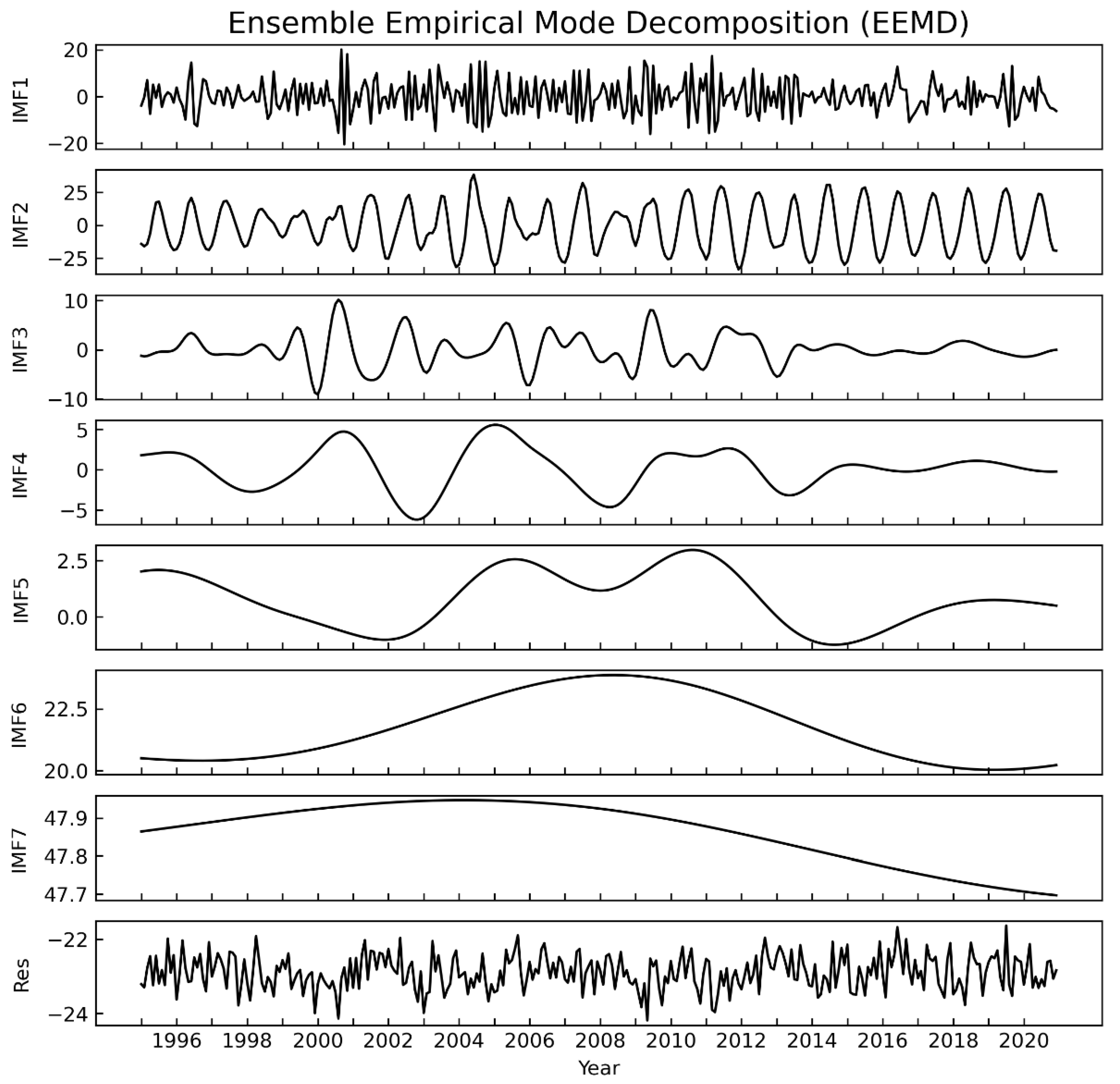
2.3.3. Ensemble Empirical Mode Decomposition (EEMD)

The empirical mode decomposition (EMD) proposed by Huang et al. [44] is a time-frequency filter that can decompose time series into modes with different timescales. To solve the problem of mode mixing in EMD, Wu and Huang [45] offered a noise-assisted analytical method named Ensemble Empirical Mode Decomposition (EEMD). Here, the EEMD was used to decompose ozone data into different empirically orthogonal intrinsic mode function (IMF) components and residuals.

3. Results

3.1. Data Sets Constructions

The ozonesonde data has the longest data record in the three ozone datasets, which is at 14:00 BJT. To keep the consistency with the ozonesonde data, the MEE ozone data at 14:00 BJT were used in this study. We also counted the number of IAGOS profiles over Beijing airport by hours (BJT) (Figure 3). It was found that IAGOS profiles were mainly available from 6:00–16:00 BJT for 1995–1999 and from 09:00–16:00 BJT for 2002–2005. There were little data available at 14:00 BJT. Therefore, we adjusted the data at other time to 14:00 BJT based on the diurnal cycle of ozone. Figure S1 shows the diurnal cycle of Beijing ozone measured by MEE in different months for 2014–2020. We assumed that ozone concentrations at other time can be adjusted to ozone at 14:00 BJT by timing a scale factor, which is month-dependent and can be estimated from the diurnal cycle of ozone in different months, as shown in Figure S1. To evaluate the method above, a comparison between the estimated and observed ozone concentrations at 14:00 BJT using the MEE ozone measurements from 2014 to 2020 is shown in Figure 4. As shown in Figure 4, the estimated ozone concentrations are very close to observed values when the time of used data is close to 14:00 BJT, but are significantly different with observed values when the time of used data is far away from 14:00 BJT. We therefore used IAGOS data from 10:00 BJT to 16:00 BJT in this study to have sufficient data and to avoid a large bias in our adjustment.

After IAGOS data adjustment, the monthly average surface ozone mixing ratio at 14:00 BJT in Beijing measured by IAGOS, ozonesonde and MEE is shown in Figure 5a. The IAGOS ozone data shown is an average between 990 hPa and the surface. The ozonesonde ozone data was averaged below 100 m. Seen from their overlap time from 2001 to 2005, the ozone values of IAGOS data are slightly higher than ozonesonde data. The ozone values in MEE data also are slightly lower than in ozonesonde during their overlapped time 2014–2019. This may be mainly because ozone concentrations below 990 hPa or below 100 m are slightly higher than only at the surface. Overall, the three ozone datasets display consistent patterns during the overlap periods. To avoid the inhomogeneity between different data, which may influence the trend estimation, we applied a linear regression between different datasets during their overlap time. For example, Figure S2 shows the ozonesonde and MEE ozone data from 2014 to 2019. Before the data correction, there were slight differences between them (Figure 5a). After performing the simple linear regression of data in the same period, the two data showed very good agreement with each other. The regression model passed a significance test at 99% confidence level. The ozonesonde data were then corrected using the MEE data as reference and the IAGOS ozone data were also corrected by such a linear regression method using the corrected ozonesonde data as reference. We finally merged the three ozone datasets and obtained a 26-year record of ozone data (at 14:00 BJT) in Beijing (Figure 5b).

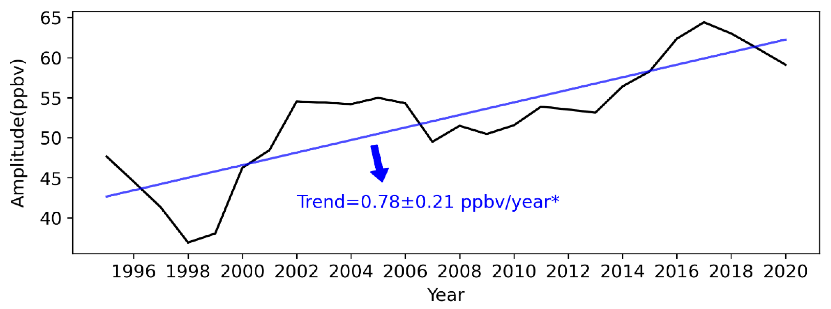
3.2. Trends of Beijing Surface Ozone

As can be seen from Figure 5b, there are some missing data in some periods. We filled the gaps in the ozone mixing ratio data by interpolation and STLForecast (see details in Section 2.3.2). Figure 6a shows the time series of ozone from 1995 to 2020 after filling the missing data points. In trend analysis, the annual cycle is usually removed before the computation. In climate change studies, the annual cycle is often estimated by the climatological mean. However, as shown in Figure 6a, the annual cycle of surface ozone in Beijing is quite different during different periods from 1995 to 2020. For example, the amplitude of annual cycle is much smaller during 1995–2000 than afterwards. Hence, the annual cycle cannot be removed well by subtracting the average of each month (Figure S3). Therefore, we applied STL to decompose the seasonal component of ozone. Indeed, Figure 6b shows that the amplitude of the annual cycle increased substantially during 1995–2020. The amplitude of the annual cycle was calculated as the difference between maximum and minimum of the STL seasonal component. The increase in annual cycle amplitude was further confirmed by the linear trend of the amplitude, as shown in Figure 7, which indicates an increase in amplitude by 0.78 ± 0.21 ppbv year⁻¹ from 1995 to 2020. The monthly ozone anomalies, which were calculated by subtracting the seasonal component as shown in Figure 6b from the initial data (Figure 6a), are displayed in Figure 6c. The long-term trend of surface ozone in Beijing was then estimated based on this time series of monthly ozone anomalies.

Surface ozone in Beijing decreased by 0.08 ± 0.12 ppbv year⁻¹ from 1995 to 2020 and the linear trend is not significant at the 95% confidence level. This is likely related to the sudden decrease in ozone in 2011–2012, which was also reported by Zhang et al. [31]. Such a steep decline in ozone is possibly related to the Clean Air Action Plan initiated nationwide in 2013 (1–2 years earlier in Beijing) and less ozone transport from the stratosphere to the troposphere [30]. We also computed the trend before 2011 and after 2013. Ozone in Beijing increased significantly by 0.42 ± 0.27 ppbv year⁻¹ during 1995–2010 and by 0.43 ± 0.41 ppbv year⁻¹ during 2013–2020, with these trends being significant at the 95% significance level. Note that the sudden drop in ozone persists until mid-2013, which makes ozone in 2013 significantly lower than after 2014. Seen from Figure 6c, ozone concentrations are almost flat after 2014. This further confirms the importance of a long-enough data record in detecting trends, since the starting/ending year strongly affects the estimated trends if the data record is short. The ozone trends calculated from monthly anomalies by removing a constant annual cycle are also shown (Figure S3). The results are in good agreement with the results shown in Figure 6c, which implies that the changes in annual cycle do not influence the long-term trend estimate significantly.

Ozone trends at 14:00 BJT in different seasons during 1995–2020 are shown in Figure 8. The surface ozone concentrations increased significantly in summer (JJA) by 0.54 ± 0.38 ppbv year⁻¹ but decreased in autumn (SON) and winter (DJF) by 0.64 ± 0.35 ppbv year⁻¹ and 0.27 ± 0.26 ppbv year⁻¹ from 1995 to 2020. In spring (MAM), the trend of ozone concentrations is close to zero and not significant. The sudden drop during 2011–2012 is also obvious in four seasons. Therefore, the linear trends of ozone in the four seasons were also calculated separately before 2011 and after 2013. During 1995–2010, ozone concentrations in Beijing show a rising trend in spring and summer, especially in summer with a significant ozone increase of 1.41 ± 0.72 ppbv year⁻¹, while a decreasing trend is seen in winter. This trend is possibly related to the rapid increase in NOx emission from 1995 to 2010 [46,47]. In summer, high temperature and solar radiation benefit the ozone photochemical process so that ozone concentration increases with increased NOx emissions [48,49]. Conversely, with the NOx concentration at a high level in winter, ozone production fell into a “NOx titrated regime” and the increased NOx emission lead to a decrease in ozone in winter [4]. The significant increase in ozone in summer and decrease in winter confirm the increase in the amplitude of the ozone annual cycle, as shown in Figure 6b and Figure 7. Anthropogenic emissions changed due to the Clean Air Plan in China after 2013 (after 2011 in Beijing). The trend of surface ozone in Beijing also changed in the four seasons. From 2013 to 2020, the surface ozone increased in all seasons except for summer, with trends of 0.67 ± 1.52 ppbv year⁻¹ in spring, 0.57 ± 0.75 ppbv year⁻¹ in autumn, and 1.12 ± 0.82 ppbv year⁻¹ in winter, respectively. It is noteworthy that the growth in ozone in winter during 2013–2020 is significant, which is caused by lower NOx emissions and reduced ozone destruction [16]. The COVID-19 lockdown in 2020 may have also enhanced this increasing trend in winter [16,50]. In summer, the ozone trend during 2013–2020 is not significant. The springtime ozone has no significant linear trend in all the three periods, with strong interannual fluctuations. Details of the ozone trends in different periods and different seasons are summarized in

Table 1. The linear trends (ppbv year⁻¹) of Beijing surface ozone mixing ratio in different periods and different seasons. The trends with “*” passed the 95% significance test.

	1995–2020	1995–2010	2013–2020
All months	−0.08 ± 0.12	0.42 ± 0.27 *	0.43 ± 0.41 *
Spring	0.02 ± 0.42	0.66 ± 0.83	0.67 ± 1.52
Summer	0.54 ± 0.38 *	1.41 ± 0.72 *	−0.02 ± 1.02
Autumn	−0.64 ± 0.35 *	0.01 ± 0.66	0.57 ± 0.75
Winter	−0.27 ± 0.26 *	−0.12 ± 0.51	1.12 ± 0.82 *

.

3.3. The Sudden Decline in Ozone during 2011–2012

As mentioned previously, there was a sudden drop in ozone in Beijing during 2011–2012. In order to explore the reasons for this sudden decline, we used CAM-chem model to simulate ozone levels from 2010–2013 (see Section 2.2 for model details). Figure 9 shows the observed and simulated ozone mixing ratio by the CMIP6 run at 14:00 BJT in Beijing. It can be seen that the values from the simulation are broadly similar to the observations. This suggests that the model can simulate the Beijing ozone level relatively well. However, the simulated slope during 2011–2012 (−0.48 ± 3.41 ppbv year⁻¹) is much weaker than that in the observation (−3.94 ± 6.31 ppbv year⁻¹). This may be caused by an unrealistic anthropogenic emission of ozone precursors in the model simulation.

The default emission of CAM-chem model is from CMIP6. However, CMIP6 emission cannot reflect the actual anthropogenic emissions in China. In Figure S4, we can see that the anthropogenic emissions of NOx over Beijing in MEIC decreases during 2010–2013 but increases in CMIP6. Due to the Chinese Air Pollution Prevention, the emissions of NOx in Beijing have declined since 2011. The MEIC-based anthropogenic emissions are more reasonable. The changes in VOCs from 2010 to 2013 are also different between MEIC and CMIP6. This deviation of emissions may lead to an inaccurate ozone simulation. We, therefore, conducted a new simulation (the MEIC run) from 2010 to 2013 using MEIC’s anthropogenic emissions of NOx and VOCs (main ozone precursors) in China, instead of CMIP6. The simulated ozone over Beijing in the MEIC run shows a more apparent decrease with −1.30 ± 2.19 ppbv year⁻¹ in 2011–2012.

To evaluate the relative contributions of meteorological conditions and anthropogenic emissions to this sudden ozone decline during 2011–2012, we employed another model simulation (the MEIC-2010 run), which fixed the anthropogenic emissions of NOx and VOCs at their 2010 values from MEIC. The ozone change during 2011–2012 in this simulation is −1.06 ± 2.41 ppbv year⁻¹. A comparison of the deseasonalized monthly anomalies of ozone from the observation and the three model simulations is shown in Figure 10. The MEIC run, in which the emission of ozone precursors decreased, shows the strongest ozone decline (−1.30 ± 2.19 ppbv year⁻¹) in the three model simulations during 2011–2012. With fixed anthropogenic emissions at the 2010 values, there is still a weaker decline in ozone (−1.06 ± 2.41 ppbv year⁻¹) in the MEIC-2010 run. In the CMIP6 run, where the emission of ozone precursors was unrealistically increasing, the ozone decline is weakest (−0.48 ± 3.41 ppbv year⁻¹). This indicates that the sudden decline in ozone in the period 2011–2012 may be mainly caused by meteorological conditions, which is consistent with the results of previous studies [30]. During 2011–2012, there was a strong La Niña event, which led to a weakening of the Brewer–Dobson circulation and less transportation of stratospheric ozone-rich air into the troposphere, therefore causing negative anomalies of tropospheric ozone at mid-latitudes [51]. Note that even the MEIC run can only simulate about 1/3 of the observed ozone decline during 2011–2012. This is possibly due to the following reasons: (1) the ability of the CAM-Chem model to simulate well the ozone changes in China; (2) the uncertainties of the anthropogenic emissions from MEIC; and (3) the uncertainties of the meteorological conditions in MERRA2, e.g., the stratosphere–troposphere exchange was not correctly estimated over this period. Although there are some uncertainties in the model simulations, it provides useful information of the relative contribution of the meteorological conditions and anthropogenic emissions to this sudden ozone decline during 2011–2012.

3.4. Interannual Variability in Surface Ozone in Beijing

Ozone is mainly produced by photochemical reactions, which are temperature- and radiation-dependent. With an average lifetime of 22.5 ± 2.2 days, ranging from a few hours in polluted urban regions up to a few weeks in the upper troposphere, ozone can also be transported from one region to another depending on atmospheric circulation [52,53]. Therefore, ozone variations at different time scales are under the influence of emissions of ozone precursors, on the one hand, and are affected by meteorological conditions and climate change, on the other hand [54,55]. Different weather and climate systems at varying time scales may produce different periodic properties in surface ozone concentrations. In order to detect the different time oscillation frequencies of Beijing surface ozone from 1995 to 2020, we used the EEMD method [45] to decompose ozone time series into multiple intrinsic mode functions (IMFs) with different timescales and a residues. The results of the EEMD method can be seen in Figure 11.

Figure 11 shows the seven IMFs of the EEMD results. IMF1 is the lowest order of EEMD, meaning the highest frequency of ozone time series. We can see that there are different periodic phenomena from IMF2 to IMF5. In order to understand the oscillation periods of IMF2–IMF5, we analyzed the power spectra, as displayed in Figure 12. The oscillation period of IMF2 is one year, which indicates the annual cycle. Tang et al. [56] suggested that the ozone concentration in Beijing is the highest in June and the lowest in December, which is in agreement with our results (Figure 6a). The abundant solar radiation and the damp air condition in summer is favorable for ozone production [57]. The maximum Beijing ozone concentration in early summer is possibly related to the East Asian summer monsoon (EASM) shifting to an earlier date [58]. There is a ~2–3 years peak in the power spectrum of IMF3 (Figure 12b), which is close to the period of the Quasi-biennial Oscillation (QBO). The QBO is the dominant mode of interannual variability in the equatorial stratosphere with a period of ~28 months. IMF4 shows a significant peak of 3~9 years (Figure 12c), which may be related to the El Niño–Southern Oscillation (ENSO). IMF5 has the periodical fluctuation of around 20 years (Figure 12d) and is possibly affected by climate systems with a longer cycle, such as the Pacific Decadal Oscillation (PDO). IMF6 and IMF7 are not periodic but show the long-term tendency of ozone. IMF6 shows an increase in the first stage before 2008 and a decrease afterwards. On much longer time scale, Beijing surface ozone mixing ratio at 14:00 BJT shows a slight decrease as displayed in IMF7, which is consistent with the long-term linear trend (Figure 6).

4. Conclusions

A long-term (26 years) ozone record for Beijing (at 14:00 BJT) was presented in this paper for the first time by merging three types of ozone measurements, i.e., IAGOS measurements, ozonesonde measurements as well as the monitoring network observations from the MEE. Using this unique data record, the long-term trend and the interannual variability in surface ozone in Beijing were explored for the period of 1995–2020. In general, the surface ozone mixing ratio at 14:00 BJT in Beijing decreased by 0.08 ± 0.12 ppbv year⁻¹ from 1995 to 2020, which is not statistically significant. This long-term trend is strongly influenced by the sudden decline in ozone concentrations in 2011–2012. Beijing ozone increased by 0.42 ± 0.27 ppbv year⁻¹ before 2011 and increased by 0.43 ± 0.41 ppbv year⁻¹ after 2013, with these increases being both statistically significant at the 95% confidence level. The trends of ozone in different seasons were also investigated. In 1995–2020, the surface ozone increased in summer but decreased in autumn and winter. Because of the increase in summer and decrease in winter, the annual cycle of ozone in Beijing became substantially strengthened from 1995 to 2020, which may cause more frequent ozone pollution episodes.

To explain the sudden drop in ozone over Beijing from 2011 to 2012, a set of model simulations were conducted using the CAM-Chem model. Because of the Clean Air Plan by the Chinese Government, the anthropogenic emissions of ozone precursors have decreased since 2013 in eastern China and since 2011 in Beijing. Using the most realistic emissions from MEIC and specified meteorological conditions from the MERRA2 reanalysis, the MEIC run simulated about 1/3 (−1.30 ± 2.19 ppbv year⁻¹) of the observed ozone decline (−3.94 ± 6.31 ppbv year⁻¹). While the emissions are fixed to 2010 values, the simulated ozone decline became weaker (−1.06 ± 2.41 ppbv year⁻¹). The run using unrealistic increasing emissions from CMIP6 showed the weakest ozone decline (−0.48 ± 3.41 ppbv year⁻¹). Although the CAM-Chem model could not simulate the ozone decrease over Beijing during 2011–2012 perfectly, a comparison of the three model simulations provided useful information of the relative contribution of anthropogenic emissions and meteorological conditions. The results indicate that the sudden ozone drop during 2011–2012 can be mainly attributed to variations in meteorological conditions, while the decrease in the anthropogenic emissions as a result of the clean air plan plays a secondary role. This is consistent with the results of previous studies [30], which found a sudden drop in ozone from the lower stratosphere to the near surface, indicating an important contribution of the weaker stratosphere-to-troposphere transport to surface ozone levels.

From the EEMD analysis, seasonal to interannual variations in Beijing surface ozone were evident from 1995 to 2020. Ozone time series can be mainly decomposed into seven modes, including periodicities of several months, one year, 2~3 years, 3~7 years, 10~20 years, and long-term trends. These periodicities are likely associated with meteorological conditions and climate systems, for example, the 2~3 years period is likely related to the QBO and the 3~7 years period is possibly related to the ENSO. The exact factors that influence the interannual variations in tropospheric ozone need further studies.

References

1. Fishman, J.; Crutzen, P.J. The origin of ozone in the troposphere. Nature 1978, 274, 855–858. [Google Scholar] [CrossRef]
2. Junge, C.E. Global ozone budget and exchange between stratosphere and troposphere. Tellus 1962, 14, 363–377. [Google Scholar] [CrossRef]
3. Stohl, A.; Bonasoni, P.; Cristofanelli, P.; Collins, W.; Feichter, J.; Frank, A.; Forster, C.; Gerasopoulos, E.; Gäggeler, H.; James, P.; et al. Stratosphere-troposphere exchange: A review, and what we have learned from STACCATO. J. Geophys. Res. Atmos. 2003, 108, D12. [Google Scholar] [CrossRef]
4. Wang, T.; Xue, L.K.; Brimblecombe, P.; Lam, Y.F.; Li, L.; Zhang, L. Ozone pollution in China: A review of concentrations, meteorological influences, chemical precursors, and effects. Sci. Total Environ. 2017, 575, 1582–1596. [Google Scholar] [CrossRef]
5. Canella, R.; Borriello, R.; Cavicchio, C.; Cervellati, F.; Martini, M.; Muresan, X.; Valacchi, G. Tropospheric ozone effects on chlorine current in lung epithelial cells: An electrophysiological approach. Free. Radic. Biol. Med. 2016, 1, S58–S59. [Google Scholar] [CrossRef]
6. Avnery, S.; Mauzerall, D.L.; Liu, J.; Horowitz, L.W. Global crop yield reductions due to surface ozone exposure: 1. Year 2000 crop production losses and economic damage. Atmos. Environ. 2011, 45, 2284–2296. [Google Scholar] [CrossRef]
7. Rider, C.F.; Carlsten, C. Air pollution and DNA methylation: Effects of exposure in humans. Clin. Epigenetics 2019, 11, 131. [Google Scholar] [CrossRef] [Green Version]
8. Van Dingenen, R.; Dentener, F.J.; Raes, F.; Krol, M.C.; Emberson, L.; Cofala, J. The global impact of ozone on agricultural crop yields under current and future air quality legislation. Atmos. Environ. 2009, 43, 604–618. [Google Scholar] [CrossRef]
9. Cooper, O.R.; Parrish, D.D.; Ziemke, J.; Balashov, N.V.; Cupeiro, M.; Galbally, I.E.; Gilge, S.; Horowitz, L.; Jensen, N.R.; Lamarque, J.-F.; et al. Global distribution and trends of tropospheric ozone: An observation-based reviewGlobal distribution and trends of tropospheric ozone. Elem. Sci. Anthr. 2014, 2, 000029. [Google Scholar] [CrossRef]
10. Staehelin, J.; Thudium, J.; Buehler, R.; Volz-Thomas, A.; Graber, W. Trends in surface ozone concentrations at Arosa (Switzerland). Atmos. Environ. 1994, 28, 75–87. [Google Scholar] [CrossRef]
11. Derwent, R.G.; Manning, A.J.; Simmonds, P.G.; Spain, T.G.; O’Doherty, S. Long-term trends in ozone in baseline and European regionally-polluted air at Mace Head, Ireland over a 30-year period. Atmos. Environ. 2018, 179, 279–287. [Google Scholar] [CrossRef] [Green Version]
12. Strode, S.A.; Rodriguez, J.M.; Logan, J.A.; Cooper, O.R.; Witte, J.C.; Lamsal, L.N.; Damon, M.; Van Aartsen, B.; Steenrod, S.D.; Strahan, S.E. Trends and variability in surface ozone over the United States. J. Geophys. Res. Atmos. 2015, 120, 9020–9042. [Google Scholar] [CrossRef]
13. Gaudel, A.; Cooper, O.R.; Ancellet, G.; Barret, B.; Boynard, A.; Burrows, J.P.; Clerbaux, C.; Coheur, P.-F.; Cuesta, J.; Cuevas, E.; et al. Tropospheric Ozone Assessment Report: Present-day distribution and trends of tropospheric ozone relevant to climate and global atmospheric chemistry model evaluation. Elem. Sci. Anthr. 2018, 6, 39. [Google Scholar] [CrossRef] [Green Version]
14. Chang, K.-L.; Petropavlovskikh, I.; Cooper, O.R.; Schultz, M.G.; Wang, T.; Helmig, D.; Lewis, A. Regional trend analysis of surface ozone observations from monitoring networks in eastern North America, Europe and East Asia. Elem. Sci. Anthr. 2017, 5, 50. [Google Scholar] [CrossRef] [Green Version]
15. Zheng, B.; Tong, D.; Li, M.; Liu, F.; Hong, C.; Geng, G.; Li, H.; Li, X.; Peng, L.; Qi, J. Trends in China’s anthropogenic emissions since 2010 as the consequence of clean air actions. Atmos. Chem. Phys. 2018, 18, 14095–14111. [Google Scholar] [CrossRef] [Green Version]
16. Li, K.; Jacob, D.J.; Liao, H.; Qiu, Y.; Shen, L.; Zhai, S.; Bates, K.H.; Sulprizio, M.P.; Song, S.; Lu, X. Ozone pollution in the North China Plain spreading into the late-winter haze season. Proc. Natl. Acad. Sci. USA 2021, 118, e2015797118. [Google Scholar] [CrossRef]
17. Lu, X.; Hong, J.; Zhang, L.; Cooper, O.R.; Schultz, M.G.; Xu, X.; Wang, T.; Gao, M.; Zhao, Y.; Zhang, Y. Severe surface ozone pollution in China: A global perspective. Environ. Sci. Technol. Lett. 2018, 5, 487–494. [Google Scholar] [CrossRef]
18. Li, K.; Jacob, D.J.; Liao, H.; Shen, L.; Zhang, Q.; Bates, K.H. Anthropogenic drivers of 2013–2017 trends in summer surface ozone in China. Proc. Natl. Acad. Sci. USA 2019, 116, 422–427. [Google Scholar] [CrossRef] [Green Version]
19. Verstraeten, W.W.; Neu, J.L.; Williams, J.E.; Bowman, K.W.; Worden, J.R.; Boersma, K.F. Rapid increases in tropospheric ozone production and export from China. Nat. Geosci. 2015, 8, 690–695. [Google Scholar] [CrossRef]
20. Xu, W.; Lin, W.; Xu, X.; Tang, J.; Huang, J.; Wu, H.; Zhang, X. Long-term trends of surface ozone and its influencing factors at the Mt Waliguan GAW station, China—Part 1: Overall trends and characteristics. Atmos. Chem. Phys. 2016, 16, 6191–6205. [Google Scholar] [CrossRef]
21. Sun, L.; Xue, L.; Wang, T.; Gao, J.; Ding, A.; Cooper, O.R.; Lin, M.; Xu, P.; Wang, Z.; Wang, X.; et al. Significant increase of summertime ozone at Mount Tai in Central Eastern China. Atmos. Chem. Phys. 2016, 16, 10637–10650. [Google Scholar] [CrossRef] [Green Version]
22. Li, J.; Lu, K.; Lv, W.; Li, J.; Zhong, L.; Ou, Y.; Chen, D.; Huang, X.; Zhang, Y. Fast increasing of surface ozone concentrations in Pearl River Delta characterized by a regional air quality monitoring network during 2006–2011. J. Environ. Sci. 2014, 26, 23–36. [Google Scholar] [CrossRef]
23. Liao, Z.; Ling, Z.; Gao, M.; Sun, J.; Zhao, W.; Ma, P.; Quan, J.; Fan, S. Tropospheric Ozone Variability Over Hong Kong Based on Recent 20 years (2000–2019) Ozonesonde Observation. J. Geophys. Res. Atmos. 2021, 126, e2020JD033054. [Google Scholar] [CrossRef]
24. Xu, X.; Lin, W.; Xu, W.; Jin, J.; Wang, Y.; Zhang, G.; Zhang, X.; Ma, Z.; Dong, Y.; Ma, Q.; et al. Long-term changes of regional ozone in China: Implications for human health and ecosystem impacts. Elem. Sci. Anthr. 2020, 8, 13. [Google Scholar] [CrossRef] [Green Version]
25. Ma, Z.; Xu, J.; Quan, W.; Zhang, Z.; Lin, W.; Xu, X. Significant increase of surface ozone at a rural site, north of eastern China. Atmos. Chem. Phys. 2016, 16, 3969–3977. [Google Scholar] [CrossRef] [Green Version]
26. Li, K.; Jacob, D.J.; Shen, L.; Lu, X.; De Smedt, I.; Liao, H. Increases in surface ozone pollution in China from 2013 to 2019: Anthropogenic and meteorological influences. Atmos. Chem. Phys. 2020, 20, 11423–11433. [Google Scholar] [CrossRef]
27. Shen, L.; Jacob, D.J.; Liu, X.; Huang, G.; Li, K.; Liao, H.; Wang, T. An evaluation of the ability of the Ozone Monitoring Instrument (OMI) to observe boundary layer ozone pollution across China: Application to 2005–2017 ozone trends. Atmos. Chem. Phys. 2019, 19, 6551–6560. [Google Scholar] [CrossRef] [Green Version]
28. Dufour, G.; Hauglustaine, D.; Zhang, Y.; Eremenko, M.; Cohen, Y.; Gaudel, A.; Siour, G.; Lachatre, M.; Bense, A.; Bessagnet, B.; et al. Recent ozone trends in the Chinese free troposphere: Role of the local emission reductions and meteorology. Atmos. Chem. Phys. 2021, 21, 16001–16025. [Google Scholar] [CrossRef]
29. Ding, A.J.; Wang, T.; Thouret, V.; Cammas, J.-P.; Nédélec, P. Tropospheric ozone climatology over Beijing: Analysis of aircraft data from the MOZAIC program. Atmos. Chem. Phys. 2008, 8, 1–13. [Google Scholar] [CrossRef] [Green Version]
30. Zhang, Y.; Tao, M.; Zhang, J.; Liu, Y.; Chen, H.; Cai, Z.; Konopka, P. Long-term variations in ozone levels in the troposphere and lower stratosphere over Beijing: Observations and model simulations. Atmos. Chem. Phys. 2020, 20, 13343–13354. [Google Scholar] [CrossRef]
31. Zhang, J.; Li, D.; Bian, J.; Xuan, Y.; Chen, H.; Bai, Z.; Wan, X.; Zheng, X.; Xia, X.; Lü, D. Long-term ozone variability in the vertical structure and integrated column over the North China Plain: Results based on ozonesonde and Dobson measurements during 2001–2019. Environ. Res. Lett. 2021, 16, 074053. [Google Scholar] [CrossRef]
32. Petzold, A.; Thouret, V.; Gerbig, C.; Zahn, A.; Brenninkmeijer, C.A.; Gallagher, M.; Hermann, M.; Pontaud, M.; Ziereis, H.; Boulanger, D.; et al. Global-scale atmosphere monitoring by in-service aircraft–current achievements and future prospects of the European Research Infrastructure IAGOS. Tellus B Chem. Phys. Meteorol. 2015, 67, 28452. [Google Scholar] [CrossRef] [Green Version]
33. Nédélec, P.; Blot, R.; Boulanger, D.; Athier, G.; Cousin, J.-M.; Gautron, B.; Petzold, A.; Volz-Thomas, A.; Thouret, V. Instrumentation on commercial aircraft for monitoring the atmospheric composition on a global scale: The IAGOS system, technical overview of ozone and carbon monoxide measurements. Tellus B Chem. Phys. Meteorol. 2015, 67, 27791. [Google Scholar] [CrossRef] [Green Version]
34. Wang, G.; Kong, Q.; Xuan, Y.; Wan, X.; Chen, H.; Ma, S. Development and application of ozonesonde system in China. Adv. Earth Sci. 2003, 18, 471–475. (In Chinese) [Google Scholar]
35. Zhang, J.; Xuan, Y.; Yan, X.; Liu, M.; Tian, H.; Xia, X.; Pang, L.; Zheng, X. Development and preliminary evaluation of a double-cell ozonesonde. Adv. Atmos. Sci. 2014, 31, 938–947. [Google Scholar] [CrossRef]
36. Xuan, Y.J.; Ma, S.Q.; Chen, H.B.; Wang, G.C.; Kong, Q.X.; Zhao, Q.; Wan, X.W. Intercomparisons of GPSO 3 and Vaisala ECC Ozone Sondes. Plateau Meteorol. 2004, 23, 394–399. (In Chinese) [Google Scholar]
37. Danabasoglu, G.; Lamarque, J.F.; Bacmeister, J.; Bailey, D.; DuVivier, A.; Edwards, J.; Emmons, L.; Fasullo, J.; Garcia, R.; Gettelman, A. The community earth system model version 2 (CESM2). J. Adv. Model. Earth Syst. 2020, 12, e2019MS001916. [Google Scholar] [CrossRef] [Green Version]
38. Emmons, L.K.; Schwantes, R.H.; Orlando, J.J.; Tyndall, G.; Kinnison, D.; Lamarque, J.F.; Marsh, D.; Mills, M.J.; Tilmes, S.; Bardeen, C.; et al. The Chemistry Mechanism in the Community Earth System Model Version 2 (CESM2). J. Adv. Model. Earth Syst. 2020, 12, e2019MS001882. [Google Scholar] [CrossRef] [Green Version]
39. Tilmes, S.; Hodzic, A.; Emmons, L.; Mills, M.; Gettelman, A.; Kinnison, D.E.; Park, M.; Lamarque, J.F.; Vitt, F.; Shrivastava, M. Climate forcing and trends of organic aerosols in the Community Earth System Model (CESM2). J. Adv. Model. Earth Syst. 2019, 11, 4323–4351. [Google Scholar] [CrossRef]
40. Feng, L.; Smith, S.J.; Braun, C.; Crippa, M.; Gidden, M.J.; Hoesly, R.; Klimont, Z.; Van Marle, M.; Van Den Berg, M.; Van Der Werf, G.R. The generation of gridded emissions data for CMIP6. Geosci. Model Dev. 2020, 13, 461–482. [Google Scholar] [CrossRef] [Green Version]
41. Li, M.; Liu, H.; Geng, G.; Hong, C.; Liu, F.; Song, Y.; Tong, D.; Zheng, B.; Cui, H.; Man, H. Anthropogenic emission inventories in China: A review. Natl. Sci. Rev. 2017, 4, 834–866. [Google Scholar] [CrossRef]
42. Wigley, T.M.; Santer, B.; Lanzante, J. Appendix A: Statistical issues regarding trends. Temp. Trends Low. Atmos. Steps Underst. Reconciling Differ. 2006, 129, 139. [Google Scholar]
43. Cleveland, R.B.; Cleveland, W.S.; McRae, J.E.; Terpenning, I. STL: A seasonal-trend decomposition. J. Off. Stat. 1990, 6, 3–73. [Google Scholar]
44. Huang, N.E.; Shen, Z.; Long, S.R.; Wu, M.C.; Shih, H.H.; Zheng, Q.; Yen, N.-C.; Tung, C.C.; Liu, H.H. The empirical mode decomposition and the Hilbert spectrum for nonlinear and non-stationary time series analysis. Proc. R. Soc. Lond. Ser. A Math. Phys. Eng. Sci. 1998, 454, 903–995. [Google Scholar] [CrossRef]
45. Wu, Z.H.; Huang, N.E. Ensemble empirical mode decomposition: A noise-assisted data analysis method. Adv. Adapt. Data Anal. 2009, 1, 1–41. [Google Scholar] [CrossRef]
46. Zhao, B.; Wang, S.; Liu, H.; Xu, J.; Fu, K.; Klimont, Z.; Hao, J.; He, K.; Cofala, J.; Amann, M. NOx emissions in China: Historical trends and future perspectives. Atmos. Chem. Phys. 2013, 13, 9869–9897. [Google Scholar] [CrossRef] [Green Version]
47. Liu, F.; Beirle, S.; Zhang, Q.; van der, A.R.; Zheng, B.; Tong, D.; He, K. NOx emission trends over Chinese cities estimated from OMI observations during 2005 to 2015. Atmos. Chem. Phys. 2017, 17, 9261–9275. [Google Scholar] [CrossRef] [Green Version]
48. Ziemke, J.R.; Chandra, S. Seasonal and interannual variabilities in tropical tropospheric ozone. J. Geophys. Res. Atmos. 1999, 104, 21425–21442. [Google Scholar] [CrossRef] [Green Version]
49. Trainer, M.; Parrish, D.; Goldan, P.; Roberts, J.; Fehsenfeld, F. Review of observation-based analysis of the regional factors influencing ozone concentrations. Atmos. Environ. 2000, 34, 2045–2061. [Google Scholar] [CrossRef]
50. Sokhi, R.S.; Singh, V.; Querol, X.; Finardi, S.; Targino, A.C.; de Fatima Andrade, M.; Pavlovic, R.; Garland, R.M.; Massagué, J.; Kong, S. A global observational analysis to understand changes in air quality during exceptionally low anthropogenic emission conditions. Environ. Int. 2021, 157, 106818. [Google Scholar] [CrossRef]
51. Kilifarska, N.A.; Velichkova, T.P.; Batchvarova, E.A. From Phase Transition to Interdecadal Changes of ENSO, Altered by the Lower Stratospheric Ozone. Remote Sens. 2022, 14, 1429. [Google Scholar] [CrossRef]
52. Griffiths, P.T.; Murray, L.T.; Zeng, G.; Shin, Y.M.; Abraham, N.L.; Archibald, A.T.; Deushi, M.; Emmons, L.K.; Galbally, I.E.; Hassler, B.; et al. Tropospheric ozone in CMIP6 simulations. Atmos. Chem. Phys. 2021, 21, 4187–4218. [Google Scholar] [CrossRef]
53. Monks, P.S.; Archibald, A.T.; Colette, A.; Cooper, O.; Coyle, M.; Derwent, R.; Fowler, D.; Granier, C.; Law, K.S.; Mills, G.E.; et al. Tropospheric ozone and its precursors from the urban to the global scale from air quality to short-lived climate forcer. Atmos. Chem. Phys. 2015, 15, 8889–8973. [Google Scholar] [CrossRef] [Green Version]
54. Fu, Y.; Liao, H.; Yang, Y. Interannual and decadal changes in tropospheric ozone in China and the associated chemistry-climate interactions: A review. Adv. Atmos. Sci. 2019, 36, 975–993. [Google Scholar] [CrossRef]
55. Fiore, A.M.; Naik, V.; Leibensperger, E.M. Air quality and climate connections. J. Air Waste Manag. Assoc. 2015, 65, 645–685. [Google Scholar] [CrossRef]
56. Tang, G.; Wang, Y.; Li, X.; Ji, D.; Hsu, S.; Gao, X. Spatial-temporal variations in surface ozone in Northern China as observed during 2009–2010 and possible implications for future air quality control strategies. Atmos. Chem. Phys. 2012, 12, 2757–2776. [Google Scholar] [CrossRef] [Green Version]
57. Chen, W.; Yan, L.; Zhao, H. Seasonal variations of atmospheric pollution and air quality in Beijing. Atmosphere 2015, 6, 1753–1770. [Google Scholar] [CrossRef] [Green Version]
58. Huang, J.; Liu, H.; Crawford, J.H.; Chan, C.; Considine, D.B.; Zhang, Y.; Zheng, X.; Zhao, C.; Thouret, V.; Oltmans, S.J.; et al. Origin of springtime ozone enhancements in the lower troposphere over Beijing: In situ measurements and model analysis. Atmos. Chem. Phys. 2015, 15, 5161–5179. [Google Scholar] [CrossRef]
59. Von Storch, H.; Zwiers, F.W. Statistical Analysis in Climate Research; Cambridge University Press: Cambridge, UK, 2002. [Google Scholar]
Figure 1. The location of Beijing airport (blue star), Nanjiao Meteorological Observatory (red triangle) and 12 sites operated by the China Ministry of Ecology and Environment (black dots). The color filling is based on terrain elevation.
Remotesensing 14 05726 g001
Figure 2. Number of IAGOS profiles (a) and the IAP ozonesonde profiles (b) over Beijing by month.
Remotesensing 14 05726 g002
Figure 3. Number of IAGOS profiles in Beijing time (BJT) by hour from 1995 to 2005.
Remotesensing 14 05726 g003
Figure 4. The relationship of ozone mixing ratio at 14:00 BJT measured by MEE and ozone mixing ratio at other time (06:00 BJT, 09:00 BJT, 10:00 BJT, 11:00 BJT, 12:00 BJT, 13:00 BJT, 15:00 BJT, 16:00 BJT, 23:00 BJT) with adjustment to 14:00 BJT. The red line is the 1:1 line.
Remotesensing 14 05726 g004
Figure 5. (a) The monthly average ozone mixing ratio in Beijing measured by IAGOS (blue, below 990 hPa), the IAP ozonesonde (red, below 100 m) and the MEE (black, surface). (b) Surface ozone mixing ratio in Beijing for 1995–2020 based on merging the three data sets (see text for details).
Remotesensing 14 05726 g005
Figure 6. (a) Monthly mean surface ozone mixing ratio in Beijing for 1995–2020 after filling missing values. (b) The seasonal component decomposed by STL from time series of surface ozone mixing ratio. (c) Monthly mean surface ozone anomalies calculated by subtracting seasonal component and its linear trends during 1995–2020 (solid blue line), before 2011 (solid green line) and after 2013 (solid red line). The trends with “*” passed the 95% significance test.
Remotesensing 14 05726 g006
Figure 7. The amplitude of the annual cycle decomposed by STL and its trend from 1995 to 2020. The “*” stands for that trend can pass the 95% significance test.
Remotesensing 14 05726 g007
Figure 8. Beijing’s surface ozone mixing ratio in (a) spring (MAM), (b) summer (JJA), (c) autumn (SON), and (d) winter (DJF). The solid blue line, green line, and red line estimate the linear trends during 1995–2020, before 2011 and after 2013. The trends with “*” passed the 95% significance test.
Remotesensing 14 05726 g008
Figure 9. Observational ozone data (black solid line) and simulated ozone mixing ratio (blue dotted line) at 14:00 BJT in Beijing during 2010–2013.
Remotesensing 14 05726 g009
Figure 10. The deseasonalized monthly anomalies of ozone in Beijing at 14:00 BJT during 2011–2012 from the observation (black line) and three model simulations by the CAM-chem model. The first set of model simulations uses the default emissions of CMIP6 (red line). The second uses MEIC’s NOx and anthropogenic VOC emissions in place of CMIP6 emissions in China (blue line). The third is based on the second emissions remaining unchanged in 2010 (cyan line).
Remotesensing 14 05726 g010
Figure 11. Ensemble empirical mode decomposition of surface ozone in Beijing with its intrinsic mode functions IMF1–IMF7 (from the lowest to the highest-order IMF) and residues.
Remotesensing 14 05726 g011
Figure 12. Power spectra of IMF2 (a), IMF3 (b), IMF4 (c), and IMF5 (d). Thick dashed lines indicate the best fit based on a first-order autoregressive model and the dotted lines indicate the 95% confidence level. The details of the power spectra and their significance tests can be seen in [59]. The dashed vertical lines show the time periods of high power, all of which pass the 95% significance test.
Remotesensing 14 05726 g012