Abstract
The previous multi-frame version of the generalized labeled multi-Bernoulli model (MF-GLMB) only accounts for standard measurement models. It is not suitable for application in the detection and tracking of multiple weak targets (low signal-to-noise ratio) due to the measurement information loss. In this paper, we introduce a MF-GLMB model that formally incorporates a track-before-detect scheme for point targets using an image sensor model. Furthermore, a belief propagation algorithm is adopted to approximately calculate the marginal association probabilities of the multi-target posterior density. In this formulation, an MF-GLMB model based on the track-before-detect measurement model (MF-GLMB-TBD smoothing) enables multi-target posterior recursion for multi-target state estimation. By taking the entire history of the state estimation into account, MF-GLMB-TBD smoothing achieves superior performance in estimation precision compared with the corresponding GLMB-TBD filter. The simulation results demonstrate that the performance of the proposed algorithm is comparable to or better than that of the Gibbs sampler-based version.
1. Introduction
Multi-target tracking inference aims at estimating trajectories from sensor data [1,2,3,4,5,6,7]. Driven by aerospace and electronic applications, multi-target tracking has become the main technique in a wide range of application areas, such as commerce and military and so on. Amongst a great deal of approaches, joint probabilistic data association (JPDA), multiple hypothesis tracking (MHT) [8], and recently random finite set (RFS) [9,10,11,12,13,14] are viewed as the three main and most prominent solutions to multi-target tracking problems. More specifically, an RFS approach based on finite set statistics (FISST) theory provides an elegant and systematic formulation for multi-target tracking. Through multi-target trajectory estimation within the Bayes framework based on the labeled RFS, it provides an analytic solution known as the generalized labeled multi-Bernoulli (GLMB) filter [1,2,3]. Further, the GLMB filter is perfectly situated to track multiple time-varying targets with tractability and fidelity using Gibbs sampler algorithm [3].
In Bayesian inference, multi-target smoothing would yield considerably better estimates than corresponding filtering due to its consideration of comprehensive state histories rather than just the current state [7,15,16]. Conditional on historical measurements including both the current measurement and previous ones, multi-target filtering works with the current state, but smoothing works with the entire history of the multi-target states up to the current multi-target state by recursively propagating the multi-target posterior. Compared to multi-target smoothing, the multi-target filtering algorithms probably suffer from phenomena such as tracking switching and track fragmentation [7]. Conversely, the posterior recursively outputted by multi-target smoothing can eliminate track switching and track fragmentation while improving previous state estimates, since it captures more comprehensive information on the multi-target trajectory. In [7], a multi-frame version of the GLMB model (MF-GLMB) is presented to accommodate (labeled) multi-target posterior recursion with respect to the standard measurement model. Meanwhile, an efficient numerical solution to multi-frame GLMB smoothing is developed for use in tracking multiple targets by computing multi-frame GLMB posterior via Gibbs sampling.
The classic detect-before-tracking (DBT) approach is implemented to make a detection decision via a thresholding operation by which a finite set of the sufficient-strength point measurements are held in reservation so as to keep the subsequent tracking approach tractable. However, this approach suffers from performance degradation due to information loss, especially for a low signal-to-noise ratio (SNR) target, whereas the TBD technique is commonly used to jointly detect and track weak targets by capturing low-SNR radar measurement. Generally, the TBD methods are roughly classified into two categories: multi-frame TBD (MF-TBD) and single-frame, recursive TBD (SFR-TBD). Efficient solutions to the MF-TBD method mainly include Hough transform (HT-TBD), maximum likelihood probabilistic data association (ML-PDA-TBD), and dynamic programming (DP-TBD) [17]. The MF-TBD methods are capable of achieving superior performance by jointly processing several consecutive frames of echo data. An alternative solution to tracking low-SNR targets is an SFR-TBD algorithm based on a pixel–image measurement model. The first SFR-TBD method was presented in [18] using a random finite set for jointly detecting multiple targets and estimating their states. In a Bayesian framework, an exact analytic estimate solution to the multi-target tracking problem is presented using the product-styled representation of labeled multi-target densities [19]. Efficient implementation of the GLMB-TBD is presented to track multiple weak targets using dynamic group strategy [20]. A multiple-mode multi-Bernoulli filter was presented to solve the tracking problem of multiple maneuvering targets [21]. A Gaussian-lattice-reduction Gibbs sampler was adopted in order to further reduce the computational cost of the GLMB-TBD filter for tracking multiple weak targets [22]. To summarize, labeled-RFS-based tracking algorithms based on TBD measurement model only involve the current state of multiple targets rather than multiple-frame states, resulting in reduced tracking performance.
In this paper, we focus on the multi-frame GLMB model for generic measurement modelling, specifically a single-frame recursive track-before-detect model (MF-GLMB-TBD). Interestingly, an MF-GLMB-TBD smoother can achieve better performance in the detection and tracking of low-SNR targets by performing smoothing while filtering. However, the MF-GLMB-TBD posterior recursion is faced with a far more serious challenge compared with standard multi-frame GLMB smoothing. On the one hand, the family of labeled RFS mixture densities outputted by the MF-GLMB-TBD algorithm is not necessarily a conjugate prior for the next recursion. In [22,23,24], the Kullback–Leibler divergence (KLD) is used to obtain tractable multi-target GLMB density approximation while preserving the cardinality distribution and the PHD of the original posterior density. On the other hand, the number of components in the posterior densities grows exponentially over time resulting in computationally intractable implementation. Consequently, the pruned methods are used to reduce the complexity by retaining components with significant weights. Thus, deterministic ranked assignment algorithms are presented to implement a GLMB-TBD filter with cubic complexity (at best) in the number of measurements [2]. More efficiently truncating algorithms such as the Gibbs sampler can improve the computational complexity with a linear scalar in the number of measurements and a quadric scalar in the number of Bernoulli components [3]. In fact, converting the mixture density to the GLMB-form density is equivalent to approximately calculating the marginal association probabilities of the joint association density. The belief propagation (BP) algorithm provides an efficient solution to computing the approximate marginal probability density function (PDF) of a high-dimensional joint probability distribution by passing messages between the neighboring nodes in the factor graph. More importantly, the BP-based approach can drastically reduce computational complexity by exploiting the condition of the statistical independencies. Therefore, the BP method is widely used in applications ranging from wireless communication [25], digital decoding [26], and target tracking [27,28]. More specifically, a fast labeled multi-Bernoulli filter (LMB) is proposed for solving probabilistic data association using belief propagation [28]. The BP-based LMB solution to the problem of multi-target tracking can further reduce complexity with better tracking precision compared to implementation based on the original truncated algorithms.
Contrary to the implementation of a multi-frame GLMB smoother based on the Gibbs sampler [7], this paper adopts the BP algorithm to implement the MF-GLMB-TBD smoother for multi-target state estimation. Collectively, the main innovations of this paper are listed as follows:
On one hand, the objective of this paper is to further generalize the multi-frame GLMB model to a pixeled image sensor model, especially for TBD measurement, thereby making it suitable for the challenging scenario of tracking multiple low-SNR targets. To this end, we introduce a generic observation model that takes into account the possible superposition of the measurements from the echo signal [18]. This paper considers a MF-GLMB smoother for the generic multi-target likelihood function in order to derive the joint implementation of the MF-GLMB-TBD smoother. The simulation results show that the proposed MF-GLMB smoother based on the TBD measurement model can effectively solve the problem of tracking multiple weak targets.
On the other hand, compared to the Gibbs sampler-based implementation of the MF-GLMB-TBD smoother, the BP-based implementation avoids the truncating of association information in order to improve the tracking precision. The Gibbs sampler-based version reduces the computational complexity of the MF-GLMB-TBD smoother by truncating Bernoulli components with insignificant weights. As a result, the relevant association information of the posterior density is ignored by the Gibbs sampler algorithm, resulting in tracking precision loss, especially when the number of samples is small. Furthermore, the complexity of the BP-based implementation scales only linearly in the number of Bernoulli components and measurements, whereas the Gibbs sampler-based solutions are quadric at best.
The rest of this paper is arranged as follows. The background of the multi-frame GLMB model is presented in Section 2. An efficient BP-based implementation of an MF-GLMB-TBD smoother is developed in Section 3. In Section 4, the convergence analysis of the BP algorithm is further discussed for solving data association in MF-GLMB-TBD smoothing. Discussion of the BP-based implementation of MF-GLMB-TBD smoothing is given in Section 5. The simulation results are given in Section 6. Concluding discussion and future research follow in Section 7.
2. Background
This section summarizes the multi-frame GLMB model, generic observation measurement (TBD) model, and KLD-based implementation of the MF-GLMB-TBD smoother. For a detailed introduction to the multi-frame GLMB model, we refer the readers to the original work [7].
2.1. Multi-Frame GLMB Model
Consider a multi-frame multi-target state in the time interval . Note that denotes the element consisting of a label and corresponding unlabeled state . Then, the multi-frame trajectory with label is the sequence of multi-target states with the same label :
where the beginning time of trajectory is denoted by
and the latest time of trajectory is given by
It is worth noting that both and are time functions of the index and . The multi-target state in the interval is defined as the concatenation of the individual target-state sequence, i.e.,
Like the analytical form of the single-frame GLMB filter, the multi-frame GLMB mode can be expressed in the so-called -GLMG form
where the multi-frame label indicator , , is non-negative with
and the multi-frame spatial density is defined on with
As shown in Equation (5), a multi-frame GLMB model can be interpreted as a mixture of multi-target component which consist of the weight and corresponding multi-frame exponential with the label history .
2.2. The Pixel-Image TBD Measurement Model
In this subsection, a multi-frame GLMB model (GLMB smoother) is developed for multi-target state estimation in the challenge scenario. The multi-frame GLMB model approaches under the standard measurement model have shown quality performance in tracking multiple targets due to their closure under Bayes recursion [7]. Similar to the single-frame GLMB version, the multi-frame GLMB model is conjugate with regard to the standard multi-target observation model. Meanwhile, the multi-frame GLMB model based on the standard multi-target likelihood lacks the capability to deal with the weak-target tracking problem. This paper introduces the pixel-imaged TBD measurement model to collect raw echo signal for updating weak-target state estimation. Figure 1 illustrates the physical scenario of the TBD measurement model. Consider a monitored region with the range . A radar with a pixel–image sensor receives the echo signal with range–Doppler–angle dimensional measurements. The collected data at the frame are modeled by the pixel–image grid to yield
where denotes the signal intensity recorded in the cell. The intensity information recorded in each cell is the echo–signal energy, i.e., , where is the complex signal with specific form
where the target template denotes a set of cells illustrated by the target with state , the measurement noise is assumed to be a white Gaussian process with zero mean and variance [23], and a point spread function will be introduced in detail as follows. The complex echo is assumed to be the target type of Swerling 0 model with
Figure 1.
The pixel-imaged observation model in three dimensions.
The TBD pixel–image plane consists of the pixel cells, where , and represent the number of range cells, Doppler cells, and angle cells, respectively. The pixel–image resolution is three-dimensional including range resolution , Doppler resolution , and angle resolution , respectively. Assume that the radar is positioned at the original point and the target state is a four-dimensional vector in Cartesian coordinates with . A target with state illustrates several cells of its neighbors. Within the effective template of the target, the echo intensity contribution from the pixel cell follows a point spread function with
where the parameters , , and in Equation (11) represent the loss coefficient in the three-dimensional measurement model. Given the target-state information in Cartesian coordinates, the physical target state in the radar interface is given by
According to [23], the likelihood ratio for the pixel–image cell is given by
where represents the modified Bessel function. Conditioned on the independent–identical–distributed (i.i.d) measurements, the multi-target likelihood function for the pixeled-image TBD model is given by
Note that the multi-target likelihood in Equation (16) preserves the entirety of the measurement information from the echo signal. Hence, by introducing a generic observation such as the TBD measurement model, the multi-frame GLMB model in [7] will be further generalized for tracking low-SNR targets.
2.3. Multi-Frame GLMBs Approximation Recursion Based on KLD
Given the multi-frame GLMB posterior density at time
For a prior density in the GLMB form as in Equation (8), applying the likelihood function (7) yields a multi-target posterior density at the next time point, resulting in a labeled RFS mixture density
where , , and
It is worth noting from Equation (18) that the posterior density is a joint density of all the targets in . This is fundamentally different from the GLMB-formed density in [1]. The mixture density (joint density) in Equation (20) would quickly tend to a computationally intractable problem, since no specific method is utilized for truncating the summation over the space of target-to-measurement associations. Consequently, the recursive posterior density does not belong to the same family at that of prior one due to the mixture densities . In order to overcome such difficulty, a possible and prudent solution to forming the closure under Bayesian recursion is to approximate the general labeled posterior density (20) by a GLMB prior. In particular, the approximated GLMB densities are numerically evaluated via the so-called -GLMB form involving explicit enumeration of the label sets. Inspired by the GLMB approximation of multi-target densities based on Kullback–Leibler divergence (KLD), such a labeled multi-target density in Equation (9) can be approximated by the GLMB-form density with
where
A salient feature of the above approximate method is the minimization of the KLD from the original distribution in Equation (11) as well as matching its PHD and cardinality distribution [24]. The number of components in the multiple-frame GLMB posterior grows exponentially with recursive time. Indeed, the main challenge to solving the above problem is determining a way to deal with data association without exhaustive enumeration. Generally, an efficient solution, based on the Gibbs sampler, to the data association problem posed by the MF-GLMB-TBD smoother is to implement multi-frame GLMB smoothing by truncating the GLMB filtering density [3]. However, the truncating performed by the Gibbs sampler would lead to tracking performance degradation in multi-target estimation precision. The main contribution of this paper is to provide an efficient algorithm for solving this data association problem.
3. An Efficient Implementation of MF-GLMB-TBD Smoother Based on Belief Propagation
In order to avoid the pruning of association information (GLMB components), we adopt an efficient technique for (approximately) calculating the marginal association probabilities based on a belief propagation algorithm. Further, an efficient BP-based solution is offered for solving the data association problem of the MF-GLMB-TBD smoother. Contrary to traditional implementation based on state-of-the-art techniques, the relevant association information is preserved using belief propagation to improve the tracking performance. Furthermore, a variant scheme based on belief propagation is used for probabilistic data association in the implementation of the MF-GLMB-TBD filter. In this regard, the GLMB RFS is reformulated by the product of its marginals in terms of a joint association distribution.
3.1. The Posterior Density Formulation of Multi-Frame GLMB Model
In order to describe the multi-frame posterior in canonical form, an extended association map : is constructed to represent each . The set of all positive one-to-one maps from to is denoted by . Consequently, can be recovered by for each . Similarly, can be completely described by the vector due to the bijection between and for each mapping . Instead of using the mapping , the association vector switch elements are defined to depict the target–measurement association. For the frame of measurement, indicates that the target with the state is associated with the measurement . indicates that the target is not associated with any measurement, and indicates a disappearing target. The set of admissible association vectors is denoted by . Similar to an admissible mapping in [26], an admissible association vector means that any measurement in is mapped to at most one target, and ensures that no measurement is assigned to more than one target. Consequently, the posterior density in Equation (9) is, in principle, approximated by
where
Note from Equation (28) that all sum only corresponds to mappings and is considered without exhaustive enumeration over all of . The weights can be further rewritten as
where the association weight is defined by
Note from Equation (31) that the weight in Equation (30) is independent of in contrast to the one in Equation (24). They are normalized with
With above reformulation, the weights can be equivalent to the probability mass function of the association vector . Specifically, the probability mass function of is mathematically defined as
With the above definition, the multi-frame GLMB posterior density can then be expressed as
According to the definition of the in Equation (33), the can be approximated by the product of its marginals with
The summation in Equation (34) can be factorized as . The product in Equation (35) can be split as . Integrating whole components, the multi-frame posterior density can be further expressed by the product with the form
where
Arriving here, we can conclude that it is MF-GLMB posterior with the weights
and corresponding spatial PDFs
The remaining problem is to approximately calculate the using a belief propagation algorithm.
3.2. The Review of the Belief Propagation
The canonical formulation of the posterior density for the multi-frame GLMB model is leveraged to construct the MF-GLMB-TBD implementation method based on belief propagation. More precisely, a fast belief propagation algorithm based on a factor graph is used to approximately calculate the marginal association probabilities involved in (39). Here, we consider the general framework of factor graphs and belief propagation.
In MF-GLMB posterior recursion, the core is closed update under GLMB prior by calculating the marginal density from the joint density with . However, direct marginalization is often computationally expensive or infeasible. According to the factorization structure of the joint posterior density function, the joint posterior density is assumed to be the product type of certain lower-dimensional factors, i.e.,
Here, the symbol represents equality up to a constant factor. Each argument consists of certain variables . Specifically, each parameter variable is denoted by a variable node, and each factor is denoted by a factor node. Meanwhile, variable node and factor node are adjacent, i.e., connected by an edge in a factor graph. Let denote the set of the label of all variables . Factor node “” passes the following message to variable node with
where denotes integration over all variables except , and is the message passed from variable node to factor node . The belief propagation would be applied to factorizations involving discrete variables by replacing the respective integrations in Equation (41) with the following summations:
The message passed from variable node to factor node is given by the product of the messages, which is passed to variable node from all adjacent factor nodes except , i.e.,
where the neighborhood set consists of the set of the labels of all those factor nodes that are adjacent to variable node . Generally, the above messages in the looping factor graph are usually repeatedly calculated in an iterative manner, and the beliefs are approximately calculated from the respective marginal posterior probability mass functions .
3.3. Message Passing Algorithm Based on Belief Propagation
We now present the belief-propagation-based solution to calculating the marginal association probabilities involved in Equation (39). Recalling the definition in Equation (33), the probability mass function is further expressed as
where association vector enforces the admissibility of the target-oriented association depicted by vector , and is defined by
Following [25] and [26], the measurement-oriented association vector is introduced in order to construct the bijectional relationship between the target and measurement. The vector consists of several non-negative value elements , where indicates that measurement is associated with target state , and means that measurement is not associated with any target. Analogously to a single association vector, the joint association probability mass function is generalized into a two-vector case, i.e.,
Here, the extended association vector enforces the admissibility of and . According to the definition of the and , the extended association vector is factorized into
where the indicator function is given by
Obviously, the indicator function describes the data association constraint. Compared to the original graph with a single association vector , the expanded graph with two association vectors and would yield an admissibility constraint due to its complete factorization. This complete factorization allows us to devise a feasible solution to calculating marginal association probabilities, albeit with redundant formulation. As discussed in [25], the redundant formulation is the basis for obtaining an efficient algorithm, resulting in a tradeoff between computational complexity and excellent estimation precision.

Figure 2.
Factor graph of (46) and (47).
3.4. Marginal Association Probability Approximation Based on Belief Propagation
The approximation calculation of the marginal association probability is conducted by performing a belief propagation algorithm on the factor graph in Figure 2. Initially, the messages are successively propagated between the factor nodes and the variable nodes and at the message passing iteration. Specifically, a message is passed from to , and another message is passed from to , respectively. It is obviously from Figure 2 that each factor node is adjacent to two variable nodes. Thus, an outgoing message from such a factor is derived according to Equation (41). We can obtain the outgoing message
and
Each message is equivalent to only two different values due to the admissibility constraint for and , i.e.,
where
To normalize the messages for compact calculation, we define via Equation (52) by dividing , i.e.,
Similarly, the normalized message is defined as
where
Further, due to the fact that all but one of the values of are one, the message is simplified as
Analogous to the above approach, the message is simplified as
Since both messages in (58) and (59) only comprise one value except for “value one”, the scalar-valued messages and containing the same information as the vector-valued messages (49) and (50) are defined as
for and . The algorithm based on Equations (60) and (61) is initialized by . Until the final iteration , the marginal association probability mass functions are approximately calculated by the beliefs at the respective variable nodes . These beliefs are given by
where
In a similar way, an approximation of is given by
A multi-target posterior density with a multi-frame GLMB form is finally obtained via approximate calculation of the beliefs according to (62) and (64).
Efficient implementation based on belief propagation is developed for computing the approximation of marginal association probability. Further, multi-target posterior recursion is performed for multi-target state estimation using a multi-frame GLMB model. A pseudocode of BP-based GLMB approximation posterior density is provided by Algorithm 1.
| Algorithm 1: BP-based GLMB approximation posterior density | ||
| Output: | ||
| For do | ||
| Calculate for as with given in (23) and for as , respectively The spatial densities for are respectively calculated according to (20) | ||
| End for | ||
| do | ||
| The message according to (60) | ||
| according to (61) | ||
| End for | ||
| The marginal are approximately calculated according to (62) and (64), respectively The update are calculated, respectively Calculate the MF-GLMB posterior density according to (38) and (39) Extract the multi-target state from the posterior density by maximum a posterior method | ||
3.5. Complexity Analysis
This subsection presents the implementation of the MF-GLMB-TBD smoothing using a BP algorithm. In [2], the implementation of MF-GLMB-TBD smoothing can be accomplished by Murty’s algorithm without exhaustive enumeration. Efficient implementation has a computational complexity of at best, where denotes the number of measurements, denotes the number of targets, and denotes the number of samplers. In [7], the computational complexity of the implementation is reduced by pruning Bernoulli components with insignificant weight, resulting in a linear complexity of the number of samplers and measurements and quadratic complexity in the number of targets, respectively. Consequently, the Gibbs-based implementation has the complexity . The computational cost of the BP-based version scales linearly with the number of iterations, measurements, and targets.
4. The Convergence Discussion on Data Association Based on Belief Propagation
This subsection discusses the convergence of the proposed BP-based version. It is necessary to establish a simplified and contractive expression in order to guarantee the convergence of the proposed BP method. According to [29], the sufficient condition of the BP algorithm is that the mapping is a contract. In general, a function is a contraction with regard to a distance measure , resulting in
For all contraction factors, . That is to say, the defined function is a contraction for arbitrary . If the function is a contraction, then any sequence formed by repeated application of will converge to the same stationed point. To this regard, the messages are measured using the dynamic range function with
without loss of generalization, both and denote the density vectors, such as , satisfying that
such that
As shown in Equations (49) and (50), the data association is an iterative form in mathematics. For notation convenience, let be the update defined in Equation (50) and be the update defined in Equation (49).
Theorem 1.
The messages updated by loopy belief propagation and converge to the same stationary point regardless of initialization.
Proof.
In fact, Theorem 1 is straightforwardly proven using contraction mapping results. The convergence of the loopy belief propagation algorithm is proven first. Given an initial , take . Note that
and
Then
where the function is defined by
On the other hand, the messages iteratively outputted by the loopy belief propagation algorithm converge to the same fixed point regardless of an initial point. Given arbitrary two starting points and , note that , , , and , then
Theorem 1 has been proven. In a word, the proposed belief propagation is efficient for solving data association with superior convergence performance in a multi-frame GLMB-TBD smoothing approach. □
5. Numerical Simulation
5.1. Simulation Setup
This section validates the tracking performance of the MF-GLMB-TBD smoothing with BP-based implementation via several simulation experiments. As shown in Figure 3, consider the multi-target tracking scenario on the two-dimensional surveillance region . The time duration is 100 sample steps in each Monte Carlo trial over which the number of targets (up to ten in total) is unknown and varies with time due to births, deaths, and crossings. The multi-target births occur around times 1, 10, 60, and 70 (s) and the multi-target deaths occur around times 30 and 50 (s), respectively. Individual target kinematics are described by a 6D state vector of position, velocity, and the complex amplitude , respectively, i.e., . Each target follows a coordinated turn model (CT) with transition density , where mean value , covariance value with
and denotes the standard deviation of the process noise, is the standard deviation of the turn rate noise, and is the amplitude fluctuation, respectively. The birth model is a labeled multi-Bernoulli RFS with the parameters where , and . The clutter is modeled as a Poisson RFS with an average intensity of . The main specific parameters in the numerical simulation are reported in Table 1.
Figure 3.
Multiple-target trajectories in the plane. Starting and stopping positions are indicated with ◯ and △, respectively. Targets become more dispersed over time.

Table 1.
Main parameters of the simulation.
In order to verify the efficacy of the proposed method in the challenge scenario, the SNR for tracking multiple targets is defined as
In the implementation of the MF-GLMB-TBD smoothing, the belief propagation version (briefly denoted by the BP-based MF-GLMB-TBD smoother) is validated in comparison to the Gibbs sampler-based version [7] (briefly denoted by the Gibbs-GLMB-TBD filter) with different values of the Bernoulli component. Due to the high degree of uncertainty in the challenging non-linear scenario with dense clutter, all of the studied filters (or smoothers) are performed using particle implementations with particles. The marginal association probabilities of the MF-GLMB-TBD approach are approximately calculated using belief propagation iterations.
5.2. Simulation Results
For a quantitative evaluation of the average performance of the tested methods, this paper adopts the Euclidean distance-based optimal sub-pattern assignment (OSPA) metric with the cutoff parameter and order to measure the deviation between the estimated and true target states. The OSPA(2) metric is also adopted to account for track switching and fragmentation.
5.2.1. Comparison with Smoother and Filter
The smoother and filter are implemented via a BP algorithm with BP iteration 20. The SNR of the target is set at 7 dB. The simulation results outputted by the tested algorithms are given as follows.
The estimated tracks outputted by the BP-MF-GLMB-TBD smoother are shown in Figure 4. It is clearly observable from Figure 4 that there are no fragmented tracks in the design of the MF-GLMB-TBD smoother. The estimated tracks outputted from the corresponding GLMB-TBD filter are shown in Figure 5. Obviously, for the corresponding filter there is a significant incidence of false, dropped, and broken tracks, and even when a track has been declared or two tracks have been crossed, the positional and localization errors are noticeably larger as compared to those of the MF-GLMB-TBD smoother. In comparison with corresponding filters, the performance of the MF-GLMB-TBD smoother is significantly better in the estimation precision since the smoother would update the entire multi-target history at each time.
Figure 4.
Ground truths for the multiple target tracking scenario and estimated tracks outputted from MF-GLMB-TBD smoother. The solid lines denote the true trajectories. The dot lines denote the estimated trajectories. The symbol ‘x’ denotes the clutter distribution.
Figure 5.
Ground truths for the multiple target tracking scenario and estimated tracks outputted from the corresponding GLMB-TBD filter. The symbol ‘x’ denotes the clutter distribution. The dot lines denote the estimated trajectories. The symbol ‘x’ denotes the clutter distribution.
The OSPA and OSPA(2) errors of both the MF-GLMB-TBD smoother and the corresponding filter’s final estimated state versus time is shown in Figure 6. The MF-GLMB-TBD smoother has the ability to correct earlier estimations since it takes the state estimate history into full consideration. Hence, its estimation error is remarkably lower than that of the corresponding filtering for the entire tracking duration, albeit at the expense of the higher computational costs. In summary, the proposed MF-GLMB-TBD smoother is superior to the corresponding filter in terms of estimation precision.
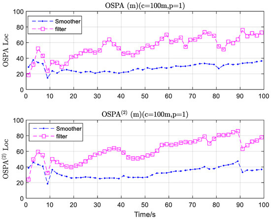
Figure 6.
OSPA and OSPA(2) error versus time for the MF-GLMB-TBD smoother and corresponding GLMB-TBD filter.
5.2.2. Comparison with BP-Version and Gibbs Sampler-Version
The number of samples used by the Gibbs sampler-based MF-GLMB-TBD smoother was set to 103 and 105, respectively. To be concise, the resulting MF-GLMB-TBD smoothers will be referred to as the Gibbs sampler-based MF-GLMB-TBD smoother-103 and the Gibbs sampler-based MF-GLMB-TBD smoother-105. Additionally, the number of BP iterations used by the BP-based MF-GLMB-TBD smoother is set to 20 and 30, respectively. The resulting MF-GLMB-TBD smoothers will be referred to as the BP-based MF-GLMB-TBD smoother-20 and the BP-based MF-GLMB-TBD smoother-30. As shown in Figure 7, the BP-based version with 30 BP iterations performs best among the four methods. Both the BP-based version with 20 BP iterations and the Gibbs sampler-based version with 105 samples are almost identical in tracking precision. Meanwhile, the Gibbs sampler-based version with 103 samples performs the worst among the four methods. The performance difference between the BP-MF-GLMB-TBD smoother and the Gibbs-MF-GLMB-TBD smoother can be explained as follows. The Gibbs-based version is performed with liner scaling of the number of measurements by truncating the GLMB components with lower weights than the threshold value. Consequently, the summations in the iterative Equation (15) are iteratively running only over the remaining Bernoulli components. Some of the relevant GLMB components are necessarily truncated resulting in ignoring relevant association information when the number of samples is small enough in the Gibbs-based version. This would directly yield a reduced tracking accuracy of the Gibbs-based version due to discarding some GLMB components with lower weights. By contrast to the Gibbs sampler-based version, the marginal association probabilities approximately calculated by the BP method completely avoid the truncating operation of the GLMB components of the posterior density resulting in improved tracking accuracy.
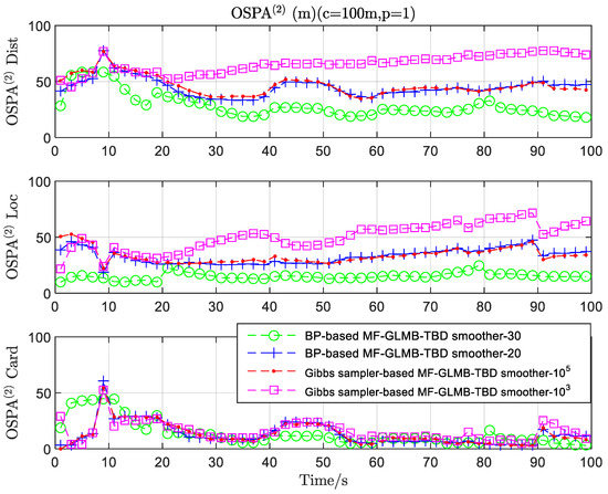
Figure 7.
OSPA(2) error versus time for the final estimation from different implementations of the MF-GLMB-TBD smoother.
In summary, the belief propagation-based version is a general case of the Gibbs sampler-based version for the implementation the MF-GLMB-TBD smoother. Selecting GLMB components with significant weights for the Gibbs sampler-based version is equivalent to drawing samples from the probability mass function . However, the BP-based version can avoid the information loss of the relevant GLMB components due to truncating performed by the Gibbs sampler version. In fact, implementation based on Gibbs sampling is a special case based on belief propagation. The performance of Gibbs sampling with a large number of Bernoulli components is almost same as that of the belief propagation with less iterative times. However, the estimate precision of the Gibbs sampling version drastically degrades as the number of Bernoulli components is reduced. Meanwhile, the performance of the belief propagation version slowly deteriorates as the iterative time is reduced.
Figure 8 plots the average runtime of the different methods, referred to as the “total runtime”. The total runtime results from Figure 8 show that the computational complex of the proposed BP-based version is significantly less than the Gibbs sampler-based version with 105 samples. The computational cost of the Gibbs sampler-based version with 103 samples is almost identical to that of the BP-based version with 20 iterations. However, the tracking precision of BP-based version with 20 iterations is remarkably better than Gibbs sampler-based version with 103 samples. Finally, as may be expected, the implementation performance of the MF-GLMB-TBD smoother based on BP is better than that based on the Gibbs sampler.
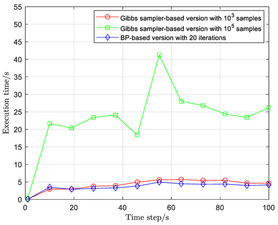
Figure 8.
The total runtime of the different methods.
6. Discussion
By incorporating the generic observation model (TBD model) into MF-GLMB smoothing, MF-GLMB-TBD smoothing is able to successfully solve the problem of tracking multiple weak targets. The positional and localization error of the MF-GLMB-TBD smoothing is considerably reduced compared with that of the MF-GLMB filter based on the standard measurement model. The complexity of MF-GLMB-TBD smoothing is far larger than that of the corresponding GLMB-TBD filter due to the full consideration of the multiple-frame state history. Hence, the current main task is to adopt a method to reduce the complexity of the implementation of the MF-GLMB-TBD smoothing. This paper uses an efficient belief propagation-based method for approximately calculating the marginal density of the posterior density in MF-GLMB-TBD smoothing. The simulation results demonstrate that the proposed BP-based implementation method is superior to the Gibbs sampler-based version, especially for challenging tracking scenarios.
7. Conclusions
Based on the multi-frame version of the GLMB model, we further generalize the results of Reference [7] to a pixel–image sensor model based on the track-before-detect strategy, thereby making it suitable for application in tracking multiple weak targets. Further, we derive the MF-GLMB-TBD posterior recursion by approximating the joint association distribution (mixture–form density) by the product of its marginals. By contrast to the Gibbs-based implementation, the approximation calculation of the GLMB posterior density using belief propagation algorithm avoids the truncating operation of the GLMB components resulting in significantly higher tracking precision. The simulation results show that the proposed BP-based implementation method outperforms the Gibbs-based version in terms of tracking precision due its preservation of all of the relevant association information. More importantly, the computational complexity of the BP-based implementation scales only linearly in the number of GLMB components and number of the measurements. The BP-based implementation achieves improved tracking performance at the cost of low computational load compared to Gibbs sampler-based version.
A multiple-sensor system would yield improved multi-target tracking performance using multi-view measurement data due to the reduction of uncertainty as to the number of targets and their states [29,30,31,32,33,34,35]. Regarding this consideration, a topic for further research is the generalization of multi-target tracking based the BP algorithm to multiple-sensor scenario. Further, another potential topic of research is how to drastically reduce the complexity of the multiple-frame GLMB model for multiple sensors.
Author Contributions
Data curation, C.C.; Formal analysis, C.C. and Y.Z.; Funding acquisition, Y.Z.; Investigation, Y.Z.; Methodology, C.C. and Y.Z.; Project administration, Y.Z.; Resources, C.C.; Supervision, Y.Z.; Writing—original draft, C.C.; Writing—review & editing, C.C. All authors have read and agreed to the published version of the manuscript.
Funding
This research was funded by 111 project, grant number No.B18039.
Conflicts of Interest
We declare that we do not have any commercial or associative interest that represents a conflict of interest in connection with the work submitted.
References
- Vo, B.T.; Vo, B.N. Labeled random finite sets and multi-object conjugate priors. IEEE Trans. Signal Process. 2013, 61, 3460–3475. [Google Scholar] [CrossRef]
- Vo, B.N.; Vo, B.T.; Phung, D. Labeled random finite sets and Bayes multi-target tracking filter. IEEE Trans. Signal Process. 2014, 62, 6554–6567. [Google Scholar] [CrossRef]
- Vo, B.N.; Vo, B.T.; Hoang, H.G. An efficient implementation of the generalized labeled multi-Bernoulli filter. IEEE Trans. Signal Process. 2017, 65, 1975–1987. [Google Scholar] [CrossRef]
- Reuter, S.; Vo, B.T.; Vo, B.N.; Dietmayer, K. The labeled multi-Bernoulli filter. IEEE Trans. Signal Process. 2014, 62, 3246–3260. [Google Scholar]
- Beard, M.; Vo, B.T.; Vo, B.N. A Solution for large-scale multi-object tracking. IEEE Trans. Signal Process. 2020, 68, 2754–2769. [Google Scholar] [CrossRef]
- Beard, M.; Vo, B.T.; Vo, B.N. Bayesian multi-target tracking with merged measurements using labeled random finite sets. IEEE Trans. Signal Process. 2015, 63, 1433–1447. [Google Scholar] [CrossRef]
- Vo, B.N.; Vo, B.T. A multi-scan labeled random finite set model for multi-object state estimation. IEEE Trans. Signal Process. 2019, 67, 4948–4963. [Google Scholar] [CrossRef]
- Blackman, S.S. Multiple hypothesis tracking for multiple target tracking. IEEE Trans. Aerosp. Electron. Syst. 2004, 19, 5–18. [Google Scholar] [CrossRef]
- Vo, B.N.; Vo, B.T.; Cantoni, A. Analytic implementations of the Cardinalized probability hypothesis density filter. IEEE Trans. Signal Process. 2007, 55, 3553–3567. [Google Scholar] [CrossRef]
- Li, C.; Wang, W.; Kirubarajan, T.; Sun, J.; Lei, P. PHD and CPHD filtering with unknown detection probability. IEEE Trans. Signal Process. 2018, 66, 3784–3798. [Google Scholar] [CrossRef]
- Jones, B.A. CPHD filter birth modeling using the probabilistic admissible region. IEEE Trans. Aerosp. Electron. Syst. 2018, 54, 1456–1469. [Google Scholar] [CrossRef]
- Mahler, R.P.S.; Vo, B.T.; Vo, B.N. CPHD filtering with unknown clutter rate and detection profile. IEEE Trans. Signal Process. 2011, 59, 3497–3513. [Google Scholar] [CrossRef]
- Bryant, D.S.; Delande, E.D.; Gehly, S.; Houssineau, J.; Clark, D.E.; Jones, B.A. The CPHD filter with target spawning. IEEE Trans. Signal Process. 2017, 65, 1324–1338. [Google Scholar] [CrossRef]
- Wang, B.; Yi, W.; Hoseinnezhad, R.; Li, S.; Kong, L.; Yang, X. Distributed fusion with multi-Bernoulli filter based on generalized covariance intersection. IEEE Trans. Signal Process. 2017, 65, 242–255. [Google Scholar] [CrossRef]
- Vo, B.T.; Clark, D.; Vo, B.N.; Ristic, B. Bernoulli forward-backward smoothing for joint target detection and tracking. IEEE Trans. Signal Process. 2011, 59, 4473–4477. [Google Scholar] [CrossRef]
- Vo, B.N.; Vo, B.T.; Mahler, R.P.S. Closed-form solutions to forward-backward smoothing. IEEE Trans. Signal Process. 2012, 60, 2–17. [Google Scholar] [CrossRef]
- Yi, W.; Fang, Z.; Li, W.; Hoseinnezhad, R.; Kong, L. Multi-frame track-before-detect algorithm for maneuvering target tracking. IEEE Trans. Veh. Technol. 2020, 69, 4104–4118. [Google Scholar] [CrossRef]
- Vo, B.N.; Vo, B.T.; Pham, N.T.; Suter, D. Joint detection and estimation of multiple objects from image observation. IEEE Trans. Signal Process. 2010, 58, 5129–5141. [Google Scholar] [CrossRef]
- Li, S.; Yi, W.; Hoseinnezhad, R.; Wang, B.; Kong, L. Multi-object tracking for generic observation using labeled random finite sets. IEEE Trans. Signal Process. 2018, 66, 368–383. [Google Scholar] [CrossRef]
- Cao, C.; Zhao, Y. An efficient implementation of multiple weak targets tracking filter with labeled random finite sets for marine radar. Digit. Signal Process. 2020, 101, 102710. [Google Scholar] [CrossRef]
- Chai, L.; Kong, L.; Li, S.; Yi, W. The multiple model multi-Bernoulli filter based track-before-detect using a likelihood based adaptive birth distribution. Signal Process. 2020, 171, 107501. [Google Scholar] [CrossRef]
- Cao, C.; Zhao, Y. An efficient implementation of the multiple-model generalized labeled multi-Bernoulli filter for track-before-detect of point targets using an image sensor. IEEE Trans. Aerosp. Electron. Syst. 2021, 57, 4416–4432. [Google Scholar] [CrossRef]
- Papi, F.; Vo, B.N.; Vo, B.T.; Fantacci, C.; Beard, M. Generalized labeled multi-Bernoulli approximation of multi-object densities. IEEE Trans. Signal Process. 2015, 63, 5487–5497. [Google Scholar] [CrossRef]
- Bryant, D.S.; Vo, B.N.; Vo, B.T.; Jones, B.A. A generalized labeled multi-Bernoulli filter with object spawning. IEEE Trans. Signal Process. 2018, 66, 6177–6189. [Google Scholar] [CrossRef]
- Li, B.; Wu, Y.-C. Convergence analysis of Gaussian belief propagation under high-order factorization and asynchronous scheduling. IEEE Trans. Signal Process 2019, 67, 2884–2897. [Google Scholar] [CrossRef]
- Leng, M.; Wu, Y.C. Distributed clock synchronization for wireless sensor networks using belief propagation. IEEE Trans. Signal Process. 2011, 59, 5404–5414. [Google Scholar] [CrossRef]
- Awais, M.; Masera, G.; Martina, M.; Montorsi, G. VLSI implementation of a non-binary decoder based on the analog digital belief propagation. IEEE Trans. Signal Process. 2014, 62, 3965–3975. [Google Scholar] [CrossRef][Green Version]
- Soldi, G.; Meyer, F.; Braca, P.; Hlawatsch, F. Self-tuning algorithms for multisensory-multitarget tracking using belief propagation. IEEE Trans. Signal Process. 2019, 67, 3922–3937. [Google Scholar] [CrossRef]
- Mooij, J.M.; Kappen, H.J. Sufficient conditions for convergence of the sum-product algorithm. IEEE Trans. Inf. Theory 2007, 53, 4422–4437. [Google Scholar] [CrossRef]
- Wien, T.; Meyer, F.; Hlawatsch, F. A fast labeled multi-Bernoulli filter using belief propagation. IEEE Trans. Aerosp. Electron. Syst. 2020, 56, 2478–2488. [Google Scholar]
- Cao, C.; Zhao, Y. A multiple-model generalized labeled multi-Bernoulli filter based on blocked Gibbs sampling for tracking maneuvering targets. Signal Process. 2021, 186, 108119. [Google Scholar] [CrossRef]
- Vo, B.N.; Vo, B.T.; Beard, M. Multi-sensor multi-object tracking with the generalized labeled multi-Bernoulli filter. IEEE Trans. Signal Process. 2019, 67, 5952–5967. [Google Scholar] [CrossRef]
- Yi, W.; Chai, L. Heterogeneous multi-sensor fusion with random finite set multi-object densities. IEEE Trans. Signal Process. 2021, 69, 3399–3414. [Google Scholar] [CrossRef]
- Garcia-Fernandez, A.F.; Yi, W. Continuous-discrete multiple target tracking with out-of-sequence measurements. IEEE Trans. Signal Process. 2021, 69, 4699–4709. [Google Scholar] [CrossRef]
- Li, S.; Battistelli, G.; Chisci, L.; Member, S.; Yi, W.; Wang, B.; Kong, L. Computationally Efficient Multi-agent multi-object tracking with labeled random finite sets. IEEE Trans. Signal Process. 2019, 67, 260–275. [Google Scholar] [CrossRef]
Publisher’s Note: MDPI stays neutral with regard to jurisdictional claims in published maps and institutional affiliations. |
© 2022 by the authors. Licensee MDPI, Basel, Switzerland. This article is an open access article distributed under the terms and conditions of the Creative Commons Attribution (CC BY) license (https://creativecommons.org/licenses/by/4.0/).