Article

Development of a New Vertical Water Vapor Model for GNSS Water Vapor Tomography

1
Jiangsu Key Laboratory of Resources and Environmental Information Engineering, China University of Mining and Technology, Xuzhou 221116, China
2
School of Environment Science and Spatial Informatics, China University of Mining and Technology, Xuzhou 221116, China
*
Author to whom correspondence should be addressed.
Remote Sens. 2022, 14(22), 5656; https://doi.org/10.3390/rs14225656
Submission received: 17 September 2022 / Revised: 26 October 2022 / Accepted: 3 November 2022 / Published: 9 November 2022
(This article belongs to the Section Atmospheric Remote Sensing)

Abstract

:
One of the main challenges of Global Navigation Satellite System (GNSS) tomography is in solving ill-conditioned system equations. Vertical constraint models are typically used in the solution procedure and play an important role in the quality of the GNSS tomography, in addition to helping resolve ill-posed problems in system equations. In this study, based on a water vapor (WV) parameter, namely IRPWV, a new vertical constraint model with six sets of coefficients for six different WV states was developed and tested throughout 2019 in the Hong Kong region with four tomographic schemes, which were carried out with the model and the traditional vertical constraint model using three different types of water vapor scale height parameters. Experimental results were numerically compared against their corresponding radiosonde-derived WV values. Compared with the tests that used the traditional model, our results showed that, first, for the daily relative error of WV density (WVD) less than 30%, the new model can lead to at least 10% and 49% improvement on average at the lower layers (below 3 km, except for the ground surface) and the upper layers (about 5–10 km), respectively. Second, the skill score of the monthly root-mean-square error (RMSE) of layered WVD above 10 accounted for about 83%, 87%, and 64%. Third, for the annual biases of layered WVD, the new model significantly decreased by 1.1–1.5 g/m3 at layers 2–3 (about 1 km), where all schemes showed the maximal bias value. Finally, for the annual RMSE of layered WVD, the new model at the lower (about 0.6–3 km) and upper layers improved by 13–42% and 5–47%, respectively. Overall, the new model performed better on GNSS tomography and significantly improved the accuracy of GNSS tomographic results, compared to the traditional model.

1. Introduction

Atmospheric water vapor (WV) is one of the most important components of the troposphere, and it plays a key role in atmospheric processes and affects almost all atmospheric processes [1], e.g., it is strongly associated with climate change, atmospheric radiation, weather patterns, and the hydrologic cycle [2,3]. Information on the distribution and variation of WV is essential for meteorological applications. Traditional WV detection techniques, such as radiosondes and automatic weather stations, can obtain WV profiles with high accuracy. However, the spatial and temporal resolution of WV cannot be described by demand in the related applications [4].
Bevis et al. [5] proposed a tropospheric tomography using meteorological Global Positioning System (GPS) networks to reconstruct three-dimensional WV fields based on GPS-derived slant delays. It made up for the shortcomings of the traditional techniques, with the advantages of low-cost, high accuracy, all weather conditions, and high temporal resolution. Hence, it has become one of the most promising techniques to reconstruct the four-dimensional distribution of atmospheric WV [6]. Plenty of Global Navigation Satellite System (GNSS) tropospheric WV tomography (GNSS tomography) studies and experiments have been carried out in different regions [7,8,9,10,11,12,13,14,15,16,17,18,19,20,21,22,23,24,25]. A GNSS tomographic domain covering the ground-based GNSS receiver network is usually cuboid-shaped or box-shaped within the troposphere, and it is first needed to discretize into many tomographic voxels in the process of tomographic solving. On account of the geographical distribution of the receivers being sparse and uneven and the geometric characteristics of the satellite constellation of GNSS, the number of satellite signals received by each receiver at a tomographic epoch is limited. In addition, all observed GNSS signal ray paths from a receiver to satellites present an inverted triangular cone shape [10,26,27,28]. Therefore, at a tomographic epoch, the number of intersecting GNSS signal rays in a voxel is insufficient and a large number of voxels are not even crossed by any rays (i.e., non-intercepted voxels), especially the bottom voxels where the WV is most active and abundant. The situations described above lead to an ill-conditioned GNSS tomographic model, i.e., the singularity condition, in which an ill-posed problem appears in the inversion of the tomographic equations, so the inverse of the design tomographic matrix cannot be directly obtained [6,7,9,29,30]. Several methods have been developed for solving the ill-posed problem, such as (1) adding inter-spatial constraints [6,8,12,13,31,32,33,34,35]; (2) adding prior information of WV [31,36,37,38]; (3) expanding the tomographic area to increase the number of available observations [19,37,39,40,41,42]; (4) using multi-GNSS observations [41,43,44,45,46,47]; (5) utilizing other observations [18,48,49,50].
In the preliminary stage of GNSS tomography, the inter-spatial constraint is a smoothing function, which uses a weighted-mean method [6,8], or the inverse-distance-weighted interpolation algorithm [19], or a Gauss distance weighting function [12]. These approaches can perform well for neighbors in the horizontal direction. However, they cannot perform effectively in the vertical direction since simple smoothing functions cannot sufficiently reflect the rapid vertical variation in the WV. Some researchers employed an exponential relationship to express the vertical relationship between the WV in nearby vertical voxels, which is under the approximation that the WV follows the ideal-gas law distribution along the vertical direction [38,51]. The exponential function performs much better than the simple weighted-mean method on constraining the vertical distribution of WV [52]. As a result, it has become the most commonly used vertical constraint model in GNSS tomography, while the exponential function is determined by the WV scale height (H), which is a key parameter of the local troposphere and is empirically determined. The vertical constraint model typically used in the solution process of GNSS tomography is not only to overcome the ill-posed problem in the inversion of the tomographic equations but also to help retrieve the vertical structure of tropospheric WV [53]. Several investigations [12,32,33,35] have shown that the performance of GNSS tomography largely depends on the accuracy of the vertical constraint conditions used in the model, especially in the case that a ground-based GNSS network is relatively flat in the height distribution of all the GNSS receivers, i.e., the geographical distribution is not optimal because of the difficulty in inverting the vertical structure of WV [8,54]. The WV varies rapidly in time and space within the troposphere, and its vertical distribution also correlates with the WV state caused by some meteorological factors, e.g., temperature and WV pressure [55]. Its vertical distribution may not always strictly follow an exponential law under different WV states, especially in the lower troposphere where WV is most active and abundant. Therefore, using the exponential relation to estimate the WV content of an empty voxel by its nearby vertical voxels under different WV states may lead to large errors.
Since the information in the variation of WV cannot be accurately detected at a high spatial and temporal resolution with current techniques, the accuracy of its fitting model may not be as good as desired under various weather conditions. One of the main issues in current GNSS tomography is the low accuracy of the vertical constraint model [13]. In this study, based on the spatio-temporal characteristics of the WV parameter, i.e., IRPWV, under different WV states, a temporal model with six sets of coefficients has been developed for the six classified WV states over the Hong Kong region. The model of IRPWV is applied as a new vertical constraint condition in the GNSS tomographic system model, and the selection of its coefficients is based on the WV state at the tomographic epoch over the tomographic region.
This paper is organized as follows. Section 2 introduces the methodology of voxel-based GNSS tropospheric WV tomography; Section 3 describes the data and processing for the GNSS tomographic experiments performed in this study, followed by the newly proposed vertical constraint model; Section 4 presents the results of the GNSS tomographic experiments and Section 5 presents concluding remarks.

2. Voxel-Based GNSS Tropospheric WV Tomography

After the retrieving of GNSS-derived slant water vapor (SWV) of each GNSS signal ray path, the continuous tomographic domain is needed to uniformly discrete into a set of three-dimensional voxels over the research area, and the continuous and varying distribution of WV over the research area is discretized by the voxels under the assumption that the WV density (WVD) in each discrete voxel is invariable, i.e., a constant, during a tomographic period, and the small influence of geometric delay in signal propagation is neglected. By discretizing the tomographic domain into a finite number of voxels, an integral signal ray path is divided into several line segments, and the full GNSS-derived SWV carried by the integral signal ray path is divided into several segments by the voxels along the signal ray path. Each segment represents the WV content of its voxel, the partial SWV, which is obtained by combining the WVD of the voxel with its corresponding signal intercept. Each partial SWV along the path of the signal ray forms a basic tomographic observation equation in discrete form. The three-dimensional WV content in the tomographic domain can be reconstructed from a large number of such signal rays during the tomographic epoch.
From the above procedure, the GNSS-derived SWV along the path of the GNSS signal in the tomographic domain during the tomographic epoch can be discretized and expressed in terms of the tomographic observation equation as
SWV s t a s a t = i , j , k m , n , l d i , j , k s t a s a t · WVD i , j , k + v
where SWV s t a s a t is the GNSS-derived SWV along the signal ray paths of the station and the satellite ( s t a s a t ); d i , j , k s t a s a t (unit: km) and WVD i , j , k (unit: g/m3) represent the distance traveled by the signal ray and the WVD within the (ith, jth, kth) voxel, respectively; the number of the voxels is m  × n × l; v is the residual term.
During the tomographic period, according to the effective signals (i.e., the signal passes through the top of the tomographic domain), the matrix form of the tomographic observation equations, which consist of all effective GNSS-derived SWV observations from all satellites observed at the GNSS station, can be written
A · X = b
where A and b are the coefficient matrix composed of the signal intercept and the column vector made up of the effective GNSS-derived SWV observations, respectively; X is the column vector of the unknown parameters that are the WVD values in each voxel.
In general, the WVD parameter in a voxel can be theoretically obtained by solving the above linear equation using least-squares estimation. However, due to the ill-posed problem of the tomographic observation equations, i.e., Equation (2) is not uniquely solvable, the horizontal and vertical constraint conditions are usually combined with Equation (2) to establish the entire GNSS tomographic equations in the following matrix form.
A A H A V · X = b 0 0
where A H is the coefficient matrix of horizontal constraint equations (e.g., the Gauss-weighted function [12] was adopted in this study); A V is the coefficient matric for vertical constraint equations, which will be introduced in Section 3.
To analyze the impact of using different vertical constraints on the GNSS tomographic result, for all tomographic schemes performed in this study, the established model of GNSS tomography was resolved under the same configurations: utilizing the singular value decomposition (SVD) method, the same horizontal constraint, and the same weighting strategy, i.e., the three types of the observations in Equation (3) were set to equal weights (the identity matrix). The only difference between different tomographic schemes is the use of different vertical constraints.

3. GNSS Tomographic Experiment

3.1. Data Description and Data Processing

Hong Kong, China, was chosen as the study area. The distribution of the Satellite Positioning Reference Station Network (SatRef) and the King’s Park radiosonde station in the tomographic region are shown in Figure 1. SatRef provides the GNSS observations for the tomographic experiments, and the radiosonde station provides meteorological profiles that are used for modeling and also as references for tomographic results.

3.1.1. GNSS Data

The Survey and Mapping Office (SMO) of Lands Department in Hong Kong, China, has applied the Global Navigation Satellite System (GNSS) to develop the local satellite positioning system, i.e., SatRef, the GNSS reference station network, which consists of 18 Continuously Operating Reference Stations (CORS), including 16 reference stations and 2 Integrity Monitoring stations evenly distributed in Hong Kong. The stations receive GNSS satellite data round-the-clock and send it to a data center for further processing and analysis. Some stations are equipped with an automatic meteorological device to record temperature, pressure, and relative humidity. The largest altitude difference among the 17 GNSS stations selected for this study is about 330 m, implying that the GNSS stations constitute a relatively flat network of GNSS reference stations.
The GNSS observations for the whole year 2019 from 17 GNSS stations were preprocessed by the Bernese software (version 5.2), and the two epochs, 00 and 12 UTC on each day, were selected as the tomographic epochs for the testing of this study, since the observing time of the radiosonde data (used as the reference) are available only at these two epochs. The following processing strategies were adopted in the usage of the software: the precise point positioning (PPP) approach [56]; a 10° cut-off elevation angle; the global mapping function (GMF) [57]; a 30-s sampling rate of GNSS data; a 1-h temporal resolution of zenith total delay (ZTD) and horizontal gradient estimates. The wet delay gradient was obtained by subtracting the dry delay gradient (the mean of 12-h tropospheric gradients) from the tropospheric gradient [58]. The ZTD and the wet delay gradient were mapped with the mapping function and then transformed into SWV by the conversion factor [5] and expressed as
SWV = Π · MF w e · ZTD ZHD + MF g e G w N S cos α + G w E W sin α + ε
where Π is the conversion factor; e and α are the elevation and azimuth angles of the ray path of the GNSS signal, respectively; MF w and MF g are the wet mapping function (GMF) and horizontal gradient mapping function [59], respectively; G w N S and G w E W are the wet gradients in the direction of north–south (NS) and east–west (EW), respectively; ε is the residual unmodeled delay along the ray path [60]; ZHD is the zenith hydrostatic delay, which can be accurately estimated by the empirical Saastamoinen model [60] and using the surface pressure at the station as the input of the model.

3.1.2. Radiosonde Data

The sounding data over the 12 years from 2008 to 2019 at the King’s Park radiosonde station were downloaded from the Integrated Global Radiosonde Archive (IGRA). The data with a 12-h temporal resolution (observed at UTC 00:00 and 12:00) can provide high-accuracy various meteorological profiles, including pressure, temperature, WV pressure, relative humidity, etc.
According to the equation of state for WV, WVD ( ρ w , unit: g/m3) can be obtained by a function of the WV partial pressure (e, unit: hPa) and temperature (T, unit: K) [61], and then PWV (unit: mm) can be calculated by the integral of WVD, expressed as
ρ w = e R T
PWV = 1 ρ v h s h t r o p ρ w d h
where R is the specific gas constant of the WV (R = 0.4615 J / K · g ); ρ v is the water density ( ρ v = 1 g/cm3); d h is the increment step (unit: km); h s and h t r o p are the heights of the ground surface and the tropopause (unit: km), respectively.
Based on the above two equations, the radiosonde-derived WVD (RS-derived WVD) profiles and PWV on each day of the year (doy) from 2008 to 2019 were calculated. Data from the first 11 years was used as the sample data to develop the vertical constraint model in Section 3.3, and data from the last year was used as a reference to validate the tomographic results.

3.2. Division Strategy for Tomographic Voxel

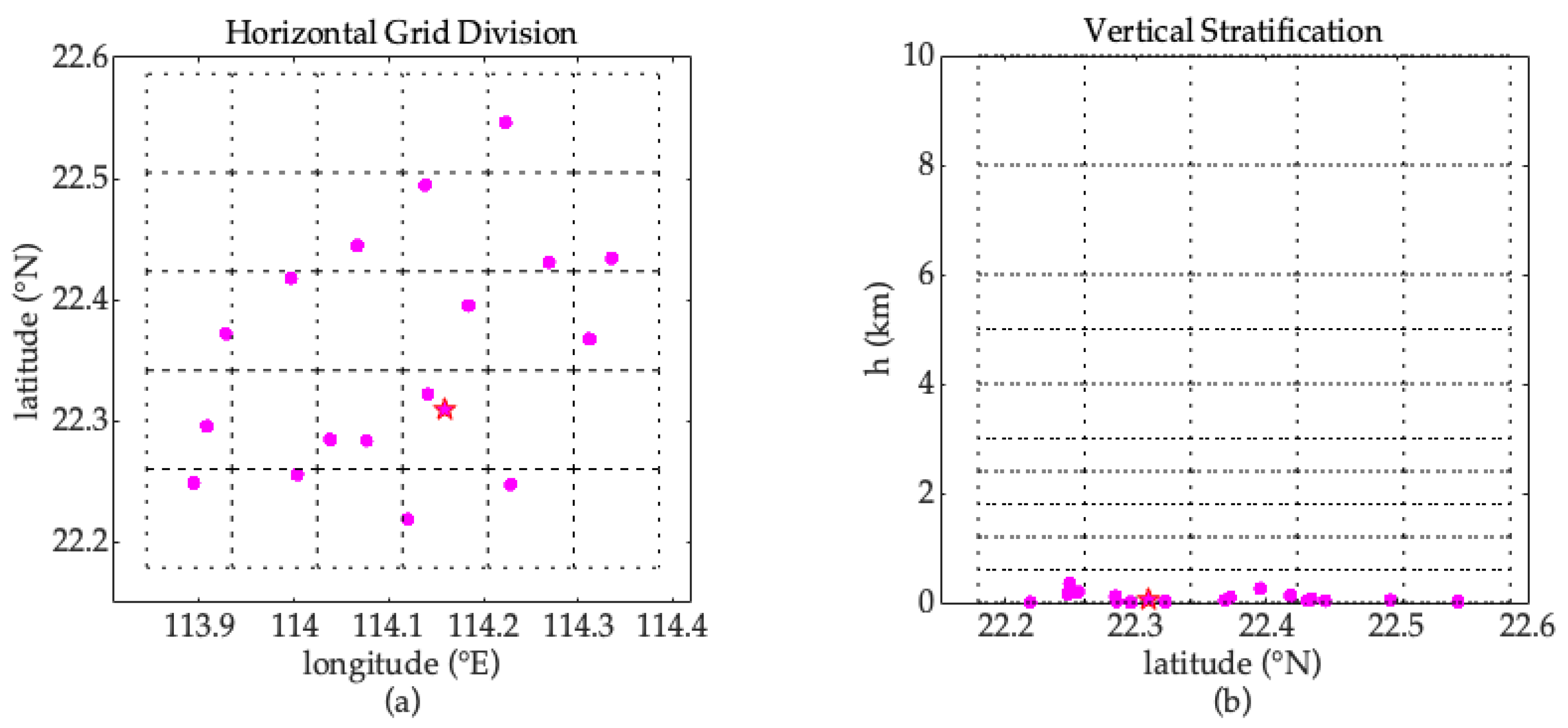
The tomographic region is from 113.81°E to 114.42°E and from 22.13°N to 22.57°N. A 0.1° interval in both longitude and latitude directions was adopted for the horizontal grid division, which yielded a 6 × 5-floor plan grid (the longitudinal and latitudinal axes were 6 and 5, respectively, as shown in the left pane of Figure 2); the troposphere over the research area is divided into 10 non-uniform layers from 0 km to the tropopause (about 10 km, where the WVD is close to 0 g/m3) along the vertical direction. Specifically, the three different height intervals were 0.6 km (below 3 km), 1 km (between 3 km and 6 km), and 2 km (above 6 km), as shown in the right pane of Figure 2. By combining the horizontal grid division and vertical layering, the tomographic domain was discretized into 6 × 5 × 10 voxels.

3.3. Vertical Constraint Conditions

3.3.1. Traditional Vertical Constraint Condition

The traditional vertical constraint condition used in GNSS tomography is an exponential function expressed as
ρ w j = ρ w i e h j h i H
where ρ w i and ρ w j are the WVD of the ith and jth layers, respectively; h i and h j are the height of the ith and jth layers, respectively; H is the WV scale height (unit: km), which can be calculated from PWV and the ground surface WVD (SWVD, ρ w s ) by
H = PWV ρ w s
The H of a local troposphere is empirically determined and usually obtained using the historical sounding data of the local radiosonde station [62]. In the application of the traditional vertical constraint, three types of H parameters are generally taken, namely, a constant, a periodic function value, and a near real-time value, which are calculated as follows: (1) Based on the sample data in Section 3.1.2, the 11-year time series of H was calculated according to Equation (8), and the mean value of H ( H m e a n ) was about 2.4 km. (2) According to the periodic nature of H [63,64], the second-order trigonometric periodic function ( H f ) was used to fit the time series, and its fitted coefficients were a H 0 = 2.6149, a H 1 = 0.0487, b H 1 = 0.0607, a H 2 = −0.0253, and b H 2 = −0.0330. (3) Some of the 17 GNSS stations were equipped with an automatic meteorological device for recording temperature, pressure, and relative humidity. Therefore, a near real-time H ( H r e a l t i m e ) was obtained by a near real-time SWVD and GNSS-derived PWV [53]. Note that if there were more than one near real-time H at a tomography epoch, then their mean would be taken as the final result.

3.3.2. Newly Proposed Vertical Constraint Model

IRPWV (unit: 1/km), derived from our previous work [65], is a WV parameter of which the vertical distribution represents the variation in WV along the vertical direction over a site in the troposphere, and it is expressed as
IRPWV h = ρ w h PWV
where ρ w h is the WVD (unit: g/m3) at the height h (unit: km).
The relationship between the WVDs at any two heights over the site is expressed in terms of their corresponding IRPWV as
ρ w j = ρ w i IRPWV j IRPWV i
where ρ w i , ρ w j , IRPWV i and IRPWV j are the WVDs and IRPWVs at h i and h j , respectively.
Based on the analysis conclusions that there is a strong correlation between the vertical structures of IRPWV and their corresponding WV states and the periodic variations in IRPWV, first, the vertical structures of IRPWV were classified into six vertical structures according to their WV states relative to the six WV states. Note that the six WV states are the states of maximal disturbance, sub-disturbance, normal, normal, sub-saturated, and saturated. Then, the spatiotemporal IRPWV model was developed at a specific height (i.e., the tomographic height layers of this study) for each of the six WV states. The spatio-temporal IRPWV models are represented in a unified form as
IRPWV h , r = a 0 , h , r + a 1 , h , r cos ( doy · w ) + b 1 , h , r sin ( doy · w ) + a 2 , h , r cos ( doy · 2 w ) + b 2 , h , r sin ( doy · 2 w )
where a 0 , h , r , a 1 , h , r , b 1 , h , r , a 2 , h , r and b 2 , h , r are the periodic coefficients; the subscript h and r are the indexes of the height layers and six WV states, respectively; w = 2 π / 365.25 .
The spatiotemporal IRPWV model was employed as a new vertical constraint model in the GNSS tomographic system equation, and its coefficients were estimated and are shown in Appendix A. The procedure for applying the new vertical constraint model to GNSS tomography is as follows: Step 1—according to the WV state at the tomographic epoch (i.e., the doy parameter), the coefficients of the new vertical constraint model are selected from the corresponding WV states (Table A2); Step 2—the coefficients and tomographic epoch are input into Equation (11) to calculate the IRPWV value at each tomographic layer; Step 3—the WVDs at any two tomographic layers along the vertical direction are expressed by Equation (10), and then the new vertical constraint equation is obtained.

4. Test Results of Using Different Vertical Constraints

In this section, WVDs resulting from the GNSS tomographic technique (hereinafter referred to as GNSS-Tom) using different vertical constraints are compared against the reference values. The GNSS-Tom experiments, with four sets of vertical constraints, are defined as different tomographic schemes, hereafter referred to as SCH1, SCH2, SCH3, and SCH4, and they are listed in Table 1.
Before comparing to the RS-derived WVD, the GNSS-Tom-derived WVD in each tomographic voxel is the mean of the WVDs in that voxel, and therefore the RS-derived WVD profile needs to be interpolated to the central position of the voxel. The interpolation method used divides the intercepted RS-derived PWV within a voxel by the height of the voxel. From the left pane of Figure 2, it can be seen that the radiosonde station is located close to the center of the grid which is in row 4 from the top to the bottom along the latitudinal direction and in column 4 from the left to the right along the longitudinal direction. Hence, the GNSS-Tom-derived WVDs in the voxels located in row 4 and column 4 of the tomographic layers 1–10 were directly used to compare against the interpolated RS-derived WVDs in the same voxel.
The GNSS-Tom-derived WVD resulting from the four tomographic schemes for each doy of 2019 is compared against the RS-derived WVD. Four statistical indicators, including relative error (RE), bias, root mean square error (RMSE), and skill score (SS), were used to evaluate the performance of the four schemes. The four metrics are defined as follows.
RE = v a l u e m o d e l i v a l u e r e f e r e n c e i v a l u e r e f e r e n c e i · 100 %
bias = 1 N i = 1 N v a l u e m o d e l i v a l u e r e f e r e n c e i
RMSE = 1 N i = 1 N v a l u e m o d e l i v a l u e r e f e r e n c e i 2
SS = 100 · 1 RMSE 1 RMSE 2
where the superscript i is the index of the sample data; the two subscripts denote the model and reference; N is the number of samples; RMSE 1 and RMSE 2 are the RMSE of experiments 1 and 2, respectively.
RE is defined as the percentage of the absolute difference between the model value and the reference value to the reference value, and in general, the smaller the RE value, the better the result. A positive SS indicates an improvement of experiment 1 over experiment 2, and the larger the SS value, the better the performance. When SS = 1, the best performance is achieved. A negative SS indicates that the application of the method (or data, or parameter, etc.) in experiment 1 had a detrimental impact. The daily RE, monthly and annual bias, and RMSE of the GNSS-Tom-derived WVD for each of the 10 tomographic layers during the 2019 tomographic experiment period, as well as the SS values for the monthly RMSEs, are all presented in the next two sections.

4.1. RE of Layered WVD

The resulting daily RE of the WVD for each of the four schemes at each of the 10 tomographic layers during 2019 is shown in Figure 3, and the information on the statistical proportion of the daily RE is given in Table 2.
It can be seen from Figure 3 that, for all the schemes, the large daily RE values (e.g., RE > 50%) are mainly distributed at the upper layers and vary with the month. The distribution of the four schemes is all the sparest in the summer and the opposite in the winter. The RE distributions of SCH1, SCH2, and SCH3 are similar, while compared to the three schemes, the large daily REs of SCH4 are more sparsely distributed in the troposphere throughout 2019.
For a more detailed analysis, the daily REs were classified empirically into two categories: RE < 30% and RE > 50%, which can distinguish the differences between the four schemes more clearly than the other categories. The statistical proportions of RE < 30% and RE > 50% of the four schemes are shown in Table 2. For RE < 30%, the higher the proportion, the better the result; whilst for RE > 50%, the higher the proportion, the worse the result.
It can be seen from Table 2 that, for all schemes, the statistical proportion of RE < 30% decreases with the increase in height layer from 1–10, which is completely different from the statistical proportion of RE > 50%. For the RE < 30% case, at layers 1–5, on average, SCH4 was 13% and 15% better than SCH1 and SCH2, respectively; it was about 10% higher than SCH3, except for layer 1, where it was 5% lower. At layers 8–10, SCH4 outperformed all the other three schemes by at least 49%. At layers 6–8, the four schemes showed similar performance. SCH4 performed slightly better than SCH1 and SCH2, and it performed slightly better than SCH3 at layer 8, but not at layers 6–7. For the RE > 50% case, the results of SCH1, SCH2, and SCH4 decreased at first and then increased with the layers from 1–3, with the returning point between layers 2 and 4 (about 1.2–1.8 km), while the results of SCH3 only showed an upward trend. In more detail, SCH4 performed better than both SCH1 and SCH2, with SCH2 slightly worse than SCH1. The four schemes performed similarly at layers 3–6. At the middle and upper layers (4–10 km), SCH4 was smaller than the other three schemes, and its reduction of statistical proportion was decreased by at least 3–22% with the increase in height layer.
Overall, the above results indicated that the results of the four tomographic schemes all performed better in summer, especially at lower altitudes than at higher altitudes. The daily RE was greater at the upper layer than at the lower layer and in winter than in summer, mainly because a small difference between a GNSS-Tom-derived WVD and its reference may result in a large absolute error relative to the reference, which also leads to a large RE value in the height/season where/when the WVD is inherently tiny, especially at the upper layers in winter.

4.2. Bias and RMSE of Layered WVD

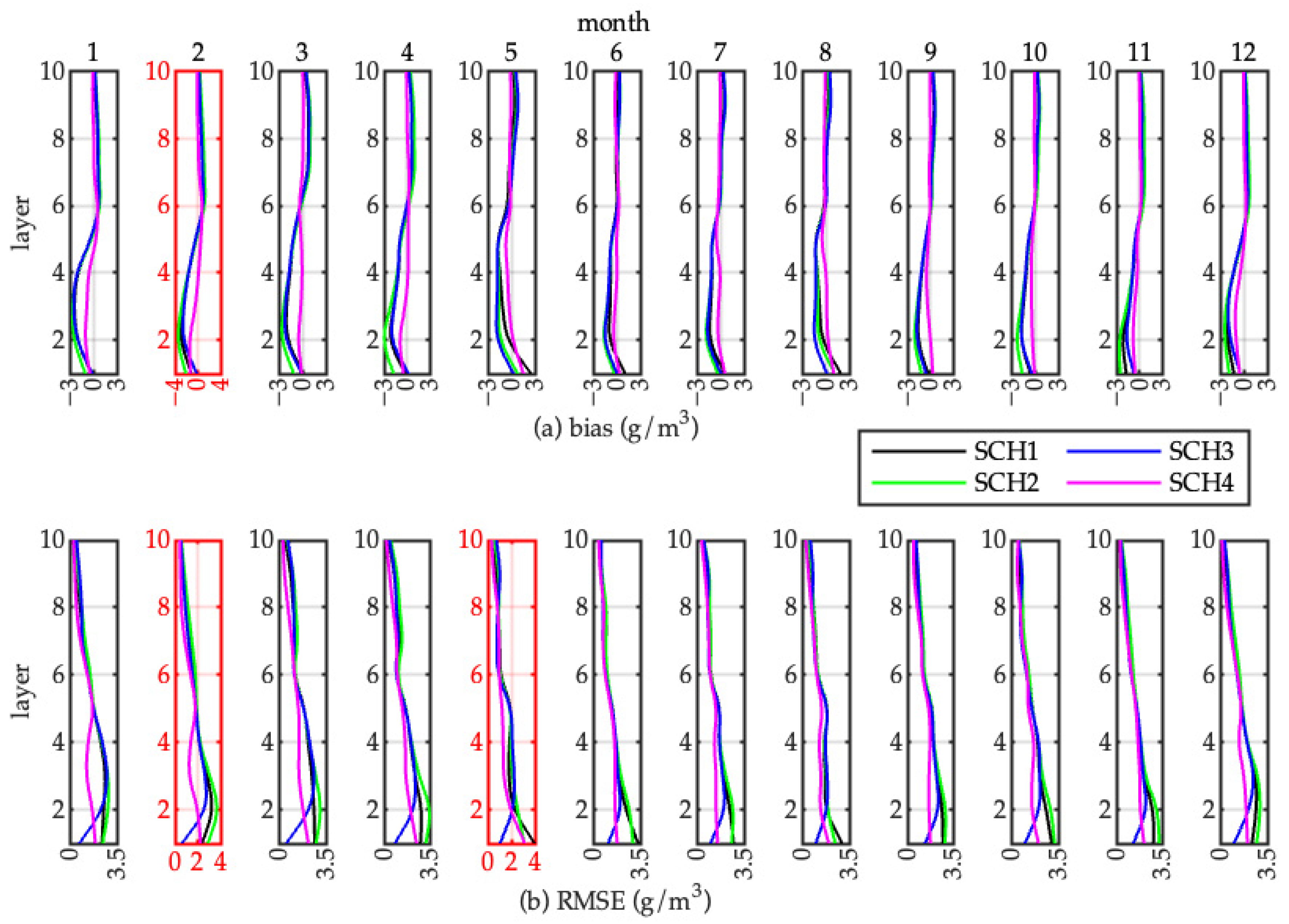
The monthly biases and RMSEs of the WVDs at each of the 10 tomographic layers resulting from each of the four schemes, as well as the skill scores (SSs) of the monthly RMSE, are shown in Figure 4 and Figure 5, respectively, during the experiment period of 2019. The results for the annual biases and RMSEs are shown in Figure 6.

4.2.1. Monthly Bias and RMSE

As can be seen from Figure 4a, the monthly biases of SCH1, SCH2, and SCH3 from 1–10 layers all presented a consistent wave shape during the 12 months of 2019, and their maximum biases occurred at layers 2–4 (about 1–2 km). All the 12 monthly biases of SCH3 at layer 1 were closer to zero than the other two schemes. Compared to the first three schemes, the monthly biases of SCH4 were around zero and slightly fluctuated with height at layers 1–10 in the 12 months, slightly varying with the variation in height. It can be seen from Figure 4b that, at layer 1, the monthly RMSEs of SCH3 were all significantly smaller than those of the other three schemes during the 12 months, wherein those of SCH4 were smaller than the remaining two schemes. At other layers, the results of SCH1, SCH2, and SCH3 were similar, while the monthly RMSEs of SCH4 were almost smaller than those of the other three schemes, except for layers 5–6, where all the schemes performed similarly. Compared to SCH1, SCH2, and SCH3, the monthly RMSEs of SCH4 were improved by at least 37%, 28%, 23%, and 21% at the lower layers (0.6–3 km), and 32%, 30%, 15%, and 18% at the upper layers (4–10 km) in the winter, spring, summer, and autumn, respectively.

4.2.2. Skill Score of Monthly RMSE

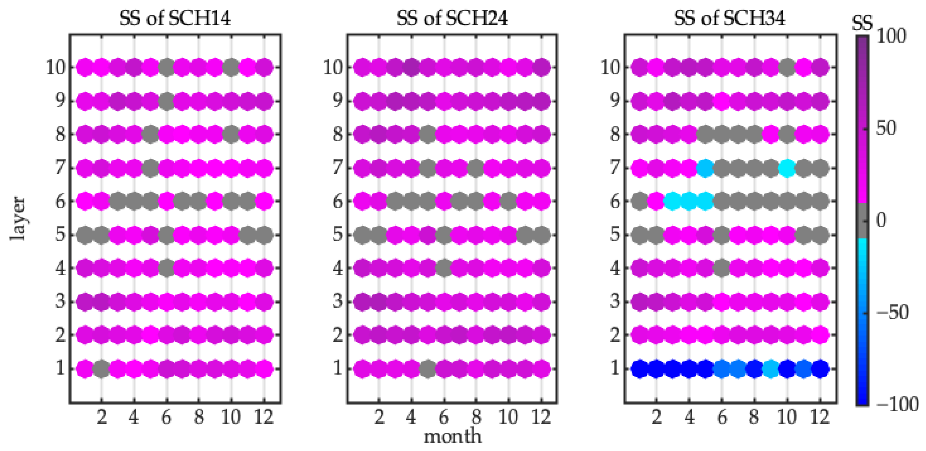
The monthly RMSEs of SCH4 and the other three schemes at each of the 10 layers were compared, and the performance of the vertical constraint model used in a tomographic scheme can be evaluated by the SS. According to Equation (15), the SS values of SCH4 relative to SCH1, SCH2, and SCH3 were obtained, namely SCH14, SCH24, and SCH34, respectively, and the results are shown in Figure 5. As we know, the only difference between the four tomographic schemes is in the vertical constraint strategy. Hence, a positive SS value indicates that the use of the new vertical constraint model proposed in this study in SCH4 is an improvement over the other three schemes. Conversely, a negative SS indicates that the assimilation of the new vertical constraint model in SCH4 has a detrimental effect. In our tomographic experiments, if the SS value was in the range of −10 to 10, then the performance of the two associated results was considered the same.
The SS values of SCH14 (left) and SCH24 (middle) in Figure 5 indicated that all the results of SCH4 were superior to those of SCH1 and SCH2. While the SSs of SCH34 revealed that SCH3 performed best at the first layer, its results at the other layers were similar to those of SCH1 and SCH2. At layers 2–5 and 8–10, the performances of SCH4 were better than those of SCH3. According to the statistics of the results from Figure 5, the numbers of SS values above 10 for SCH14, SCH24, and SCH34 were about 83%, 87%, and 64%, respectively. More specifically, the SS values at layers 1–4 of SCH14 and SCH24 were almost all above 10 with the mean of 30 and 32, respectively. Their values at layers 7–10 and 5–6 were approximately 25 and 33, and 11 and 10, respectively. The means of the SS values at layers 2–4 and 9–10 of SCH34 were about 28 and 40, respectively, and the values at layers 5, 7, and 8 were all about 10 on average.

4.2.3. Annual Bias and RMSE

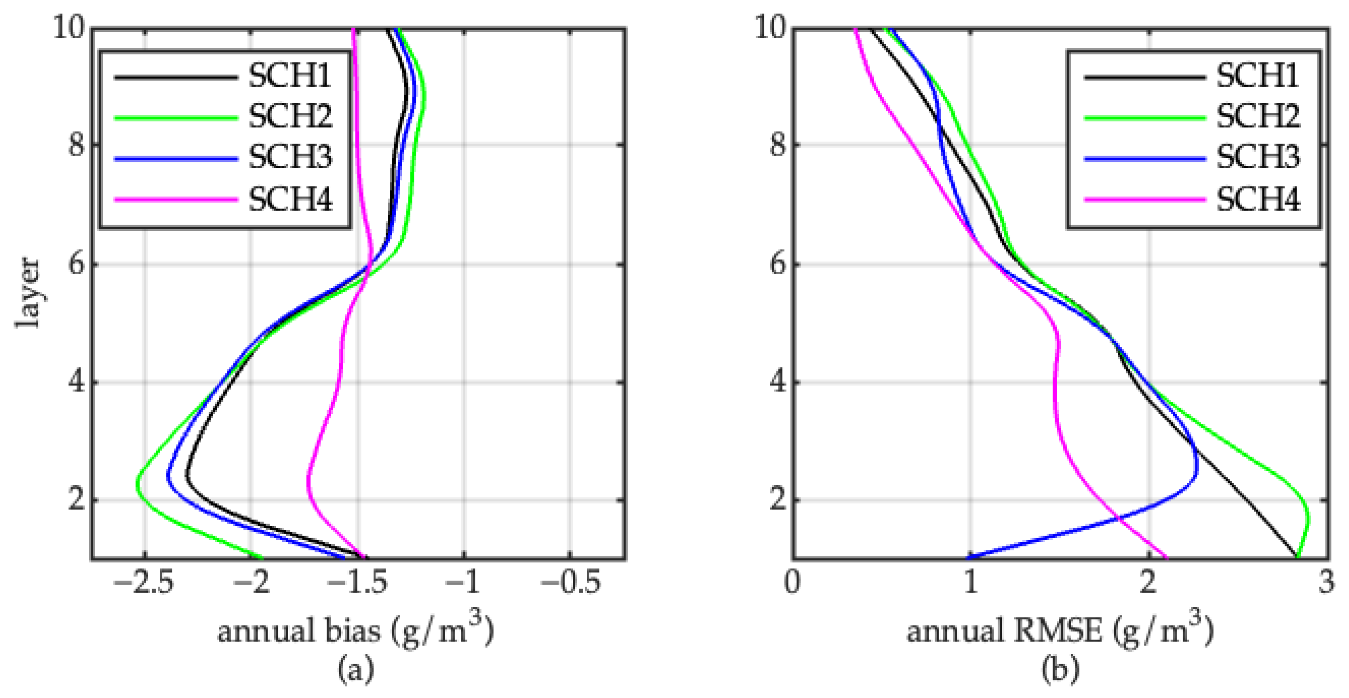
From Figure 6a, compared with the other three schemes, the annual bias of SCH4 was closest to zero from the first to the last layers, and its largest absolute bias was at layers 2–3, with a value of about −0.5 g/m3. The other three schemes all showed a notable systematic deviation, and the signs of systematic deviations at layers 2–5 were the opposite of those of layers 7–9. Although all four schemes showed a large annual bias between layers 2 and 3 (about 1 km), the annual bias of SCH4 significantly decreased by 1.1–1.5 g/m3 compared to those of the other three schemes. In Figure 6b, the annual RMSEs of SCH4 at layers 1–6 and layers 7–10 have improvements of 23–34% and 13–42%, and 9–37% and 10–47%, respectively, over those of SCH1 and SCH2, while they outperformed those of SCH3 at layers 2–6 and 7–10 by 12–35% and 5–45%, respectively.
The monthly and annual layered results indicated that, first, the tomographic results of SCH4, which used the new model, were more stable than the other three schemes, which used the traditional vertical constraint model. The new model is a linear relationship between WVDs at different heights along the vertical direction. Unlike the exponential relationship expressed by the traditional vertical model, the new model can well reflect the relationship of WVs at different heights, even in the case that the WVD varies rapidly at a specific height in the troposphere, without the occurrence of very unreliable WV values. Secondly, the accuracy of the new model result significantly outperformed the other three schemes at both the lower layers (0.6–3 km) and upper layers (4–10 km) in all 12 months. The selection of the coefficient for the new model is based on the WV state at the tomographic epoch. As a result, its tomographic result agrees with the water vapor distribution better than the traditional model. Thirdly, at the middle layers (3–4 km), the new model performs similarly to the traditional models, which is mainly because the signs of the systematic errors in the tomographic results of SCH1, SCH2, and SCH3 at the lower layers are completely different from those at the upper layers, i.e., if the systematic errors are negative values at the lower layer, then they will be positive values at the upper layer. Thus, the systematic errors at the middle layers are most likely to be close to zero, which leads to the same performance of SCH1, SCH2, and SCH3 as SHC4 at these layers. It should be noted that the good result of SCH3 at layer 1 (ground surface) is due to its usage of near real-time H parameter calculated from real-time WV. At the other layers, however, the results of SCH3 are comparable to SCH1 and SCH2. Overall, the significantly better performance of SCH4 than the other three schemes suggests the effectiveness of the new model.

5. Conclusions

With the development of GNSS tomography for nearly 20 years, one of the main challenges of GNSS tomography has been to solve ill-conditioned model equations. Vertical constraint models are typically used in the solution process and play an important role in the quality of the GNSS tomography, in addition to resolving ill-posed problems in the system equations. In this study, based on the IRPWV parameter, a new vertical constraint model with six sets of coefficients was developed for the six classified WV states over the tomographic region for improving the accuracy of GNSS tomography, since the new model can provide a good representation of the vertical variation in the WV of the local troposphere under various WV states.
To test the performance of the new vertical constraint model on GNSS tomography, tomographic experiments with four tomographic schemes were carried out using GNSS-derived WV from 17 GNSS stations in Hong Kong, China throughout 2019. The first tomographic scheme used the new model (scheme 4, namely SCH4), and the other three schemes employed the traditional vertical constraint with three different types of water vapor scale height (H), i.e., a constant (scheme 1, namely SCH1), a periodic function (scheme 2, namely SCH2), and a near real-time value (scheme 3, namely SCH3). The results of the four schemes were compared against their corresponding radiosonde-derived WV density (WVD), and the results of the four schemes were compared on three different time scales: daily, monthly, and annual.
The results showed that the daily relative errors (RE) of all four schemes at the lower layer were smaller than those at the upper layer, especially in summer. This is mainly because the RE is sensitive to small values; even a tiny deviation will result in a large RE. For the case of the daily RE of WVD of less than 30%, the results of SCH4 were 13% and 15% on average better than those of SCH1 and SCH2 at the lower layers (below 3 km), respectively; they were about 10% higher than those of SCH3 at the same layers, except for the ground surface, where they were 5% lower. The four schemes showed similar performance at the middle layers (4–5), while at the upper layers (5–10 km), SCH4 outperformed all the other three schemes by at least 49%. It should be noted that the usage of the real-time WV value is the only reason for the higher accuracy of SCH3 at layer 1; hence, this will be taken into account in the development of an improved vertical constraint model in future.
The monthly biases of SCH4 were almost zero at all layers (1–10) within all 12 months, while that of SCH1, SCH2, and SCH3 were smaller than the reference at the lower layers and larger at the upper layers, which is mainly due to the systematic deviation of the traditional models. In contrast, the SCH4 result had no obvious deviation from the reference because the selection of the new model is based on the characteristics of water vapor at different heights under different water vapor states. The monthly RMSEs of SCH4 at the lower layers (0.6–3 km) were reduced at least by 37%, 28%, 23%, and 21% and at the middle and upper layers (4–10 km) by 32%, 30%, 15%, and 18% in the winter, spring, summer, and autumn, respectively. Additionally, the monthly skill scores of SCH4 can reflect the performance of the new model. By comparing the monthly layered RMSEs of SCH4 relative to those of SCH1, SCH2, and SCH3, the statistics of skill scores above 10 in the new model accounted for 83%, 87%, and 64%, respectively. Similar results were observed in the annual results as well as the monthly results. Although all four schemes showed the maximal annual absolute bias was at layers 2 and 3 (about 1 km), the annual bias of SCH4 was about −0.5 g/m3, and it significantly decreased by 1.1–1.5 g/m3 in comparison to those of the other schemes. The annual RMSEs of SCH4 compared with SCH1 and SCH2 at layers 1–6 (the ground surface to 3 km) decreased by 23–34% and 13–42%, respectively, and at the other layers (3–10 km) by 9–37% and 10–47%, respectively. Compared with SCH3, the annual RMSEs of SCH4 at layers 2–6 (0.6–3 km) and 7–10 (4–10 km) decreased by 12–35% and 5–45%, respectively.
All evaluation results demonstrate the better performance of the new model than the traditional ones. Based on the spatiotemporal distribution of the WV at different heights for different WV states, the new model obtained from the classification statistical analysis is more refined. In its application, the selection of an appropriate new vertical constraint model is based on the state of the WV at the current tomographic epoch over the tomographic region. The better performance of the new model compared to the traditional model, which is roughly a vertical constraint condition with a simple empirical value for the H parameter, suggests that the new model better reflects the vertical distribution of the WV over the tomographic region at the tomographic epoch. Our future work will focus on the construction and testing of new models for different weather conditions or regions.

Author Contributions

All authors contributed to the study’s conception and design. Material preparation, data collection, and analysis were performed by M.W. The first draft of the manuscript was written by M.W. and all authors commented on previous versions of the manuscript. All authors have read and agreed to the published version of the manuscript.

Funding

This research was funded by the Natural Science Foundation of China (Grant No. 42274021), the Construction Program of Space-Air-Ground-Well Cooperative Awareness Spatial Information Project (Grant No. B20046), the Independent Innovation Project of “DoubleFirst Class” Construction. (Grant No. 2022ZZCX06), and the State Key Program of the National Natural Science Foundation of China [Grant No. 41730109].

Data Availability Statement

The radiosonde data can be downloaded from https://www.ncdc.noaa.gov/data-access/weather-balloon/integrated-global-radiosonde-archive (accessed on 10 December 2021). The ground-based GNSS observation data and meteorological products can be downloaded from the Satellite Positioning Reference Station Network (SatRef), Hong Kong, China, at https://www.geodetic.gov.hk (accessed on 10 December 2021).

Acknowledgments

We acknowledge the Hong Kong Geodetic Survey Service for providing GNSS data and the National Oceanic and Atmospheric Administration (NOAA) for the provision of the Integrated Global Radiosonde Archive (IGRA) datasets.

Conflicts of Interest

The authors declare no conflict of interest.

Appendix A

According to the results of the correlation between the vertical distribution of IRPWV and the relative magnitude of its corresponding PWV at a certain time, it is necessary to establish a PWV partitioning criterion to compare and determine the relative magnitude of PWV in the same time scale, and six PWV ranges criteria were proposed [65]. Note that the six PWV ranges (from 1 to 6) are considered as six water vapor states: maximal disturbance, sub-disturbance, normal, normal, sub-saturated, and saturated, respectively. Based on the periodic characteristics of the PWV time series, the fitting models of PWV ( PWV f ) and its standard deviation ( SD f ) were established by the sample data of PWV in Section 3.1.2. Wherein PWV f is the fitting periodic function of RS-derived PWV time series, SD f is the standard deviation of the fitting periodic function of RS-derived PWV, and they were calculated by a second-order trigonometric periodic function of which the fitting periodic coefficients were shown in Table A1. The time series of six PWV ranges were expressed by PWV f and SD f on each doy as [less than PWV f doy SD f doy , PWV f doy SD f doy ], [ PWV f doy SD f doy , PWV f doy 0.5 · SD f doy ], [ PWV f doy 0.5 · SD f doy , PWV f doy ], [ PWV f doy , PWV f doy + 0.5 · SD f doy ], [ PWV f doy + 0.5 · SD f doy , PWV f doy + SD f doy ] and [ PWV f doy + SD f doy , greater than PWV f doy + SD f doy ].
Table A1. Periodic coefficients of the second-order trigonometric periodic function of PWV and SD.
a 0 a 1 b 1 a 2 b 2
PWV f 42.90−16.97−4.18−1.50−0.92
SD f 8.670.68−0.750.01−1.02
Based on the sample data in Section 3.1.2, the 11-year IRPWV data were calculated by the WVD profiles and RS-derived PWV by Equation (9), and according to the six PWV ranges time series, they were first partitioned by the relative magnitude of their corresponding RS-derived PWV and then grouped to 10 height ranges by the vertical layering strategies of the tomographic grid division in Section 3.2. In consideration of the main annual and semi-annual periodic characteristics of the IRPWV time series, a third-order trigonometric periodic function was adopted as its fitting function. The temporal modeling for each of the height ranges of the 11-year IRPWV data is carried out, and its coefficients are presented in Table A2. In application, at a tomographic epoch, according to the relative magnitude of the mean of all the GNSS-derived PWV to the six PWV ranges, the periodic function coefficients of the corresponding PWV range are selected from Table A2. Note that the height of all the GNSS stations is in the first tomographic layer in this study, as well as the radiosonde station. Herein, the mean of all the GNSS-derived PWV is used. The specific design and usage of the spatiotemporal IRPWV model can be found in Wan et al. [65].
Table A2. Six sets of coefficients of the new vertical constraint model for the six classified WV states at the 10 tomographic layers corresponding to six PWV ranges (from 1–6) at the radiosonde station in Hong Kong, China.
Coefficient
of
PWV Range
Tomographic Layer
12345678910
1 a 0 0.4780.3630.2490.1830.1300.0880.0470.0260.0130.005
a 1 0.0300.011−0.0180.0000.007−0.005−0.011−0.0050.0000.000
b 1 −0.002−0.017−0.0060.0010.0120.0020.0000.0010.0020.001
a 2 0.0200.003−0.0160.0200.003−0.012−0.007−0.0020.0000.000
b 2 0.0080.0010.0110.005−0.001−0.004−0.0050.000−0.0010.000
a 3 −0.014−0.017−0.0050.0160.008−0.002−0.0020.0030.0020.000
b 3 0.0120.0120.013−0.006−0.010−0.011−0.003−0.001−0.0010.000
2 a 0 0.4090.3430.2740.2150.1470.0940.0490.0270.0110.003
a 1 0.0120.0190.0300.0160.009−0.019−0.021−0.010−0.003−0.001
b 1 −0.012−0.0060.0100.0110.0100.002−0.007−0.003−0.0010.000
a 2 0.0160.0080.0070.009−0.005−0.014−0.0080.0010.0010.000
b 2 0.0060.0070.0100.0110.003−0.006−0.008−0.003−0.0020.000
a 3 −0.003−0.005−0.0010.0050.000−0.0040.0020.0010.0010.000
b 3 0.0010.0030.005−0.001−0.004−0.0030.0010.000−0.0010.000
3 a 0 0.3870.3380.2700.2160.1530.0990.0520.0280.0120.004
a 1 0.0080.0270.0320.0210.011−0.018−0.020−0.014−0.005−0.001
b 1 −0.0130.0020.0120.0110.008−0.001−0.007−0.004−0.0010.000
a 2 0.0110.0060.0070.007−0.001−0.011−0.005−0.0010.0010.000
b 2 −0.0020.0020.0120.0150.000−0.007−0.007−0.002−0.0010.000
a 3 0.0030.0010.0020.0040.000−0.005−0.0010.0000.0000.000
b 3 −0.001−0.0010.0040.001−0.003−0.0040.0020.0020.0000.000
4 a 0 0.3650.3250.2650.2180.1570.1050.0560.0310.0140.004
a 1 0.0030.0250.0370.0250.017−0.014−0.022−0.016−0.007−0.002
b 1 −0.0010.0120.0120.0070.004−0.005−0.010−0.005−0.0020.000
a 2 0.0060.0030.0060.005−0.001−0.009−0.0060.0000.0010.001
b 2 0.0070.0130.0100.0070.000−0.008−0.007−0.003−0.0010.000
a 3 −0.001−0.0020.0000.003−0.002−0.0020.0010.0010.0000.000
b 3 0.0000.0030.002−0.0010.000−0.0070.0000.0020.0010.000
5 a 0 0.3470.3100.2570.2150.1570.1120.0640.0370.0160.005
a 1 0.0000.0200.0310.0240.017−0.006−0.016−0.015−0.009−0.003
b 1 0.0010.0160.0150.0100.006−0.004−0.010−0.006−0.003−0.001
a 2 −0.002−0.0040.0030.0020.000−0.003−0.0030.0000.0000.000
b 2 0.0060.0100.0090.0060.004−0.007−0.008−0.004−0.0010.000
a 3 −0.003−0.005−0.0020.000−0.0010.0030.0010.0020.0000.000
b 3 −0.001−0.0010.0010.002−0.001−0.0030.0010.0010.0010.000
6 a 0 0.3210.2930.2440.2090.1550.1210.0740.0440.0200.006
a 1 −0.0100.0130.0220.0180.0130.004−0.007−0.012−0.009−0.004
b 1 0.0050.0170.0130.0100.005−0.004−0.008−0.008−0.004−0.001
a 2 −0.007−0.0040.0010.0020.0000.004−0.0020.0000.0000.000
b 2 0.0050.0090.0060.0040.002−0.003−0.006−0.004−0.0010.000
a 3 −0.006−0.009−0.005−0.001−0.0020.0030.0040.0030.0010.000
b 3 0.000−0.001−0.002−0.002−0.002−0.002−0.0010.0020.0010.000

References

  1. Chahine, M.T. The Hydrological Cycle and Its Influence on Climate. Nature 1992, 359, 373–380. [Google Scholar] [CrossRef]
  2. Held, I.M.; Soden, B.J. Robust Responses of the Hydrological Cycle to Global Warming. J. Clim. 2006, 19, 5686–5699. [Google Scholar] [CrossRef]
  3. Niell, A.E.; Coster, A.J.; Solheim, F.S.; Mendes, V.B.; Toor, P.C.; Langley, R.B.; Upham, C.A. Comparison of Measurements of Atmospheric Wet Delay by Radiosonde, Water Vapor Radiometer, GPS, and VLBI. J. Atmos. Ocean. Technol. 2001, 18, 830–850. [Google Scholar] [CrossRef]
  4. Champollion, C.; Masson, F.; Bouin, M.N.; Walpersdorf, A.; Doerflinger, E.; Bock, O.; Van Baelen, J. GPS Water Vapour Tomography: Preliminary Results from the ESCOMPTE Field Experiment. Atmos. Res. 2005, 74, 253–274. [Google Scholar] [CrossRef] [Green Version]
  5. Bevis, M.; Businger, S.; Herring, T.A.; Rocken, C.; Anthes, R.A.; Ware, R.H. GPS Meteorology: Remote Sensing of Atmospheric Water Vapor Using the Global Positioning System. J. Geophys. Res. 1992, 97, 15787. [Google Scholar] [CrossRef]
  6. Flores, A.; Ruffini, G.; Rius, A. 4D Tropospheric Tomography Using GPS Slant Wet Delays. Ann. Geophys. 2000, 18, 223–234. [Google Scholar] [CrossRef]
  7. Seko, H.; Shimada, S.; Nakamura, H.; Kato, T. Three-Dimensional Distribution of Water Vapor Estimated from Tropospheric Delay of GPS Data in a Mesoscale Precipitation System of the Baiu Front. Earth Planets Space 2000, 52, 927–933. [Google Scholar] [CrossRef] [Green Version]
  8. Flores, A.; De Arellano, J.V.G.; Gradinarsky, L.P.; Rius, A. Tomography of the Lower Troposphere Using a Small Dense Network of GPS Receivers. IEEE Trans. Geosci. Remote Sens. 2001, 39, 439–447. [Google Scholar] [CrossRef]
  9. Gradinarsky, L.; Jarlemark, P. GPS Tomography Using the Permanent Network in Göteborg: Simulations. In Proceedings of the Record—IEEE PLANS, Position Location and Navigation Symposium, Palm Springs, CA, USA, 15–18 April 2002; pp. 128–133. [Google Scholar]
  10. Troller, M.; Bürki, B.; Cocard, M.; Geiger, A.; Kahle, H.-G. 3-D Refractivity Field from GPS Double Difference Tomography. Geophys. Res. Lett. 2002, 29, 2-1–2-4. [Google Scholar] [CrossRef]
  11. Nilsson, T.; Gradinarsky, L. Water Vapor Tomography Using GPS Phase Observations: Simulation Results. IEEE Trans. Geosci. Remote Sens. 2006, 44, 2927–2941. [Google Scholar] [CrossRef]
  12. Song, S.; Zhu, W.; Ding, J.; Peng, J. 3D Water-Vapor Tomography with Shanghai GPS Network to Improve Forecasted Moisture Field. Chin. Sci. Bull. 2006, 51, 607–614. [Google Scholar] [CrossRef]
  13. Perler, D.; Geiger, A.; Hurter, F. 4D GPS Water Vapor Tomography: New Parameterized Approaches. J. Geod. 2011, 85, 539–550. [Google Scholar] [CrossRef] [Green Version]
  14. Manning, T.; Zhang, K.; Rohm, W.; Choy, S.; Hurter, F. Detecting Severe Weather Using GPS Tomography: An Australian Case Study. J. Glob. Position. Syst. 2012, 11, 59–70. [Google Scholar] [CrossRef]
  15. Rohm, W.; Zhang, K.; Bosy, J. Unconstrained, Robust Kalman for GNSS Troposphere Tomography. Atmos. Meas. Tech. 2013, 6, 9133–9162. [Google Scholar] [CrossRef] [Green Version]
  16. Chen, B.; Liu, Z. Voxel-Optimized Regional Water Vapor Tomography and Comparison with Radiosonde and Numerical Weather Model. J. Geod. 2014, 88, 691–703. [Google Scholar] [CrossRef]
  17. Manning, T.; Rohm, W.; Zhang, K.; Hurter, F.; Wang, C. Determining the 4D Dynamics of Wet Refractivity Using GPS Tomography in the Australian Region; Springer: Berlin/Heidelberg, Germany, 2013; Volume 139, pp. 41–49. [Google Scholar]
  18. Chen, B.; Liu, Z. Assessing the Performance of Troposphere Tomographic Modeling Using Multi-Source Water Vapor Data during Hong Kong’s Rainy Season from May to October 2013. Atmos. Meas. Tech. 2016, 9, 5249–5263. [Google Scholar] [CrossRef] [Green Version]
  19. Ding, N.; Zhang, S.B.; Wu, S.Q.; Wang, X.M.; Zhang, K.F. Adaptive Node Parameterization for Dynamic Determination of Boundaries and Nodes of GNSS Tomographic Models. J. Geophys. Res. Atmos. 2018, 123, 1990–2003. [Google Scholar] [CrossRef]
  20. Zhao, Q.; Yao, W.; Yao, Y.; Li, X. An Improved GNSS Tropospheric Tomography Method with the GPT2w Model. GPS Solut. 2020, 24, 1–13. [Google Scholar] [CrossRef]
  21. Liu, C.; Yao, Y.; Xu, C. Conventional and Neural Network-Based Water Vapor Density Model for GNSS Troposphere Tomography. GPS Solut. 2022, 26, 4. [Google Scholar] [CrossRef]
  22. Mousavian, R.; Hossainali, M.; Lorenz, C.; Kunstmann, H. Copula, a New Approach for Optimum Design of Voxel-Based GNSS Tropospheric Tomography Based on the Atmospheric Dynamics. GPS Solut. 2022, 26, 149. [Google Scholar] [CrossRef]
  23. Sadeghi, E.; Hossainali, M.; Safari, A. Development of a Hybrid Tomography Model Based on Principal Component Analysis of the Atmospheric Dynamics and GPS Tracking Data. GPS Solut. 2022, 26, 77. [Google Scholar] [CrossRef]
  24. Adavi, Z.; Weber, R.; Glaner, M.F. Assessment of Regularization Techniques in GNSS Tropospheric Tomography Based on Single- and Dual-Frequency Observations. GPS Solut. 2022, 26, 21. [Google Scholar] [CrossRef]
  25. Wilgan, K.; Hurter, F.; Geiger, A.; Rohm, W.; Bosy, J. Tropospheric Refractivity and Zenith Path Delays from Least-Squares Collocation of Meteorological and GNSS Data. J. Geod. 2017, 91, 117–134. [Google Scholar] [CrossRef] [Green Version]
  26. Mishra, M.R.; Behera, R.K.; Jha, S.; Panda, A.K.; Mishra, A.; Pradhan, D.K.; Choudary, P.R. A Brief Review on Phytoconstituents and Ethnopharmacology of Scoparia Dulcis Linn. (Scrophulariaceae). Int. J. Phytomedicine 2011, 3, 422–438. [Google Scholar] [CrossRef]
  27. Bender, M.; Raabe, A. Preconditions to Ground Based GPS Water Vapour Tomography. Ann. Geophys. 2007, 25, 1727–1734. [Google Scholar] [CrossRef]
  28. Rohm, W. The Precision of Humidity in GNSS Tomography. Atmos. Res. 2012, 107, 69–75. [Google Scholar] [CrossRef]
  29. Haji-Aghajany, S.; Amerian, Y.; Verhagen, S. B-Spline Function-Based Approach for GPS Tropospheric Tomography. GPS Solut. 2020, 24, 88. [Google Scholar] [CrossRef]
  30. Haji-Aghajany, S.; Amerian, Y.; Verhagen, S.; Rohm, W.; Schuh, H. The Effect of Function-Based and Voxel-Based Tropospheric Tomography Techniques on the GNSS Positioning Accuracy. J. Geod. 2021, 95, 78. [Google Scholar] [CrossRef]
  31. Troller, M.; Geiger, A.; Brockmann, E.; Bettems, J.M.; Bürki, B.; Kahle, H.G. Tomographic Determination of the Spatial Distribution of Water Vapor Using GPS Observations. Adv. Space Res. 2006, 37, 2211–2217. [Google Scholar] [CrossRef]
  32. Zhang, K.; Manning, T.; Wu, S.; Rohm, W.; Silcock, D.; Choy, S. Capturing the Signature of Severe Weather Events in Australia Using GPS Measurements. IEEE J. Sel. Top. Appl. Earth Obs. Remote Sens. 2015, 8, 1839–1847. [Google Scholar] [CrossRef]
  33. Mateus, P.; Miranda, P.M.A.; Nico, G.; Catalão, J.; Pinto, P.; Tomé, R. Assimilating InSAR Maps of Water Vapor to Improve Heavy Rainfall Forecasts: A Case Study With Two Successive Storms. J. Geophys. Res. Atmos. 2018, 123, 3341–3355. [Google Scholar] [CrossRef]
  34. Yao, Y.; Xin, L.; Zhao, Q. An Improved Pixel-Based Water Vapor Tomography Model. Ann. Geophys. 2019, 37, 89–100. [Google Scholar] [CrossRef] [Green Version]
  35. Zhang, M.; Zhang, K.; Wu, S.; Shi, J.; Li, L.; Wu, H.; Liu, S. A New Method for Tropospheric Tomography Using GNSS and Fengyun-4A Data. Atmos Res 2022, 280, 106460. [Google Scholar] [CrossRef]
  36. Notarpietro, R.; Cucca, M.; Gabella, M.; Venuti, G.; Perona, G. Tomographic Reconstruction of Wet and Total Refractivity Fields from GNSS Receiver Networks. Adv. Space Res. 2011, 47, 898–912. [Google Scholar] [CrossRef]
  37. Yao, Y.; Zhao, Q. Maximally Using GPS Observation for Water Vapor Tomography. IEEE Trans. Geosci. Remote Sens. 2016, 54, 7185–7196. [Google Scholar] [CrossRef]
  38. Benevides, P.; Catalao, J.; Nico, G.; Miranda, P.M.A. 4D Wet Refractivity Estimation in the Atmosphere Using GNSS Tomography Initialized by Radiosonde and AIRS Measurements: Results from a 1-Week Intensive Campaign. GPS Solut. 2018, 22, 91. [Google Scholar] [CrossRef]
  39. Rohm, W. The Ground GNSS Tomography-Unconstrained Approach. Adv. Space Res. 2013, 51, 501–513. [Google Scholar] [CrossRef]
  40. Zhao, Q.; Yao, Y. An Improved Troposphere Tomographic Approach Considering the Signals Coming from the Side Face of the Tomographic Area. Ann. Geophys. 2017, 35, 87–95. [Google Scholar] [CrossRef] [Green Version]
  41. Zhao, Q.; Yao, Y.; Yao, W.; Xia, P. An Optimal Tropospheric Tomography Approach with the Support of an Auxiliary Area. Ann. Geophys. 2018, 36, 1037–1046. [Google Scholar] [CrossRef] [Green Version]
  42. Yang, F.; Guo, J.; Shi, J.; Zhao, Y.; Zhou, L.; Song, S. A New Method of GPS Water Vapor Tomography for Maximizing the Use of Signal Rays. Appl. Sci. 2019, 9, 1446. [Google Scholar] [CrossRef]
  43. Benevides, P.; Nico, G.; Catalao, J.; Miranda, P.M.A. Analysis of Galileo and GPS Integration for GNSS Tomography. IEEE Trans. Geosci. Remote Sens. 2017, 55, 1936–1943. [Google Scholar] [CrossRef]
  44. Dong, Z.; Jin, S. 3-D Water Vapor Tomography in Wuhan from GPS, BDS and GLONASS Observations. Remote Sens. 2018, 10, 62. [Google Scholar] [CrossRef] [Green Version]
  45. Zhao, Q.; Yao, Y.; Cao, X.; Yao, W.Q. Accuracy and Reliability of Tropospheric Wet Refractivity Tomography with GPS, BDS, and GLONASS Observations. Adv. Space Res. 2019, 63, 2836–2847. [Google Scholar] [CrossRef]
  46. Zhang, W.; Zhang, S.; Ding, N.; Holden, L.; Wang, X.; Zheng, N. GNSS-RS Tomography: Retrieval of Tropospheric Water Vapor Fields Using GNSS and RS Observations. IEEE Trans. Geosci. Remote Sens. 2021, 60, 1–13. [Google Scholar] [CrossRef]
  47. Xiong, S.; Ma, F.; Ren, X.; Chen, J.; Zhang, X. LEO Constellation-Augmented Multi-GNSS for 3D Water Vapor Tomography. Remote Sens. 2021, 13, 3056. [Google Scholar] [CrossRef]
  48. Benevides, P.; Nico, G.; Catalão, J.; Miranda, P.M.A. Bridging InSAR and GPS Tomography: A New Differential Geometrical Constraint. IEEE Trans. Geosci. Remote Sens. 2016, 54, 697–702. [Google Scholar] [CrossRef]
  49. Jaberi Shafei, M.; Mashhadi-Hossainali, M. Application of the GNSS-R in Tomographic Sounding of the Earth Atmosphere. Adv. Space Res. 2018, 62, 71–83. [Google Scholar] [CrossRef]
  50. Miranda, P.M.A.; Mateus, P. A New Unconstrained Approach to GNSS Atmospheric Water Vapor Tomography. Geophys. Res. Lett. 2021, 48, e2021GL094852. [Google Scholar] [CrossRef]
  51. Elósegui, P.; Ruis, A.; Davis, J.L.; Ruffini, G.; Keihm, S.J.; Bürki, B.; Kruse, L.P. An Experiment for Estimation of the Spatial and Temporal Variations of Water Vapor Using GPS Data. Phys. Chem. Earth 1998, 23, 125–130. [Google Scholar] [CrossRef]
  52. Cao, Y. GPS Tomographying Three-Dimensional Atmospheric Water Vapor and Its Meteorological Applications. Ph.D. Thesis, The Chinese Academy of Sciences, Beijing, China, 2012. [Google Scholar]
  53. Xia, P.; Ye, S.; Jiang, P.; Pan, L.; Guo, M. Assessing Water Vapor Tomography in Hong Kong with Improved Vertical and Horizontal Constraints. Ann. Geophys. 2018, 36, 969–978. [Google Scholar] [CrossRef]
  54. Haji-Aghajany, S.; Amerian, Y.; Verhagen, S.; Rohm, W.; Ma, H. An Optimal Troposphere Tomography Technique Using the WRF Model Outputs and Topography of the Area. Remote Sens. 2020, 12, 1442. [Google Scholar] [CrossRef]
  55. Jacob, D. The Role of Water Vapour in the Atmosphere. A Short Overviewfrom a Climate Modeller’s Point of View. Phys. Chem. Earth Part A Solid Earth Geod. 2001, 26, 523–527. [Google Scholar] [CrossRef]
  56. Andritsch, F.; Dach, R.; Grahsl, A.; Schildknecht, T.; Jäggi, A. Bernese GNSS Software Version 5.2. User manual; Astronomical Institute, University of Bern, Bern Open Publishing: Bern, Switzerland, 2015. [Google Scholar]
  57. Boehm, J.; Niell, A.; Tregoning, P.; Schuh, H. Global Mapping Function (GMF): A New Empirical Mapping Function Based on Numerical Weather Model Data. Geophys. Res. Lett. 2006, 33, 7. [Google Scholar] [CrossRef] [Green Version]
  58. Bar-Sever, Y.E.; Kroger, P.M.; Borjesson, J.A. Estimating Horizontal Gradients of Tropospheric Path Delay with a Single GPS Receiver. J. Geophys. Res. Solid Earth 1998, 103, 5019–5035. [Google Scholar] [CrossRef] [Green Version]
  59. Chen, G.; Herring, T.A. Effects of Atmospheric Azimuthal Asymmetry on the Analysis of Space Geodetic Data. J. Geophys. Res. Solid Earth 1997, 102, 20489–20502. [Google Scholar] [CrossRef]
  60. Shoji, Y.; Nakamura, H.; Iwabuchi, T.; Aonashi, K.; Seko, H.; Mishima, K.; Itagaki, A.; Ichikawa, R.; Ohtani, R. Tsukuba GPS Dense Net Campaign Observation: Improvement in GPS Analysis of Slant Path Delay by Stacking One-Way Postfit Phase Residuals. J. Meteorol. Soc. Jpn. 2004, 82, 301–314. [Google Scholar] [CrossRef] [Green Version]
  61. Tomasi, C. Determination of the Total Precipitable Water by Varying the Intercept in Reitan’s Relationship. J. Appl. Meteorol. 1981, 20, 1058–1069. [Google Scholar] [CrossRef]
  62. Ye, S.; Xia, P.; Cai, C. Optimization of GPS Water Vapor Tomography Technique with Radiosonde and COSMIC Historical Data. Ann. Geophys. 2016, 34, 789–799. [Google Scholar] [CrossRef] [Green Version]
  63. Kennett, E.J.; Toumi, R. Temperature Dependence of Atmospheric Moisture Lifetime. Geophys. Res. Lett. 2005, 32, 1–4. [Google Scholar] [CrossRef]
  64. Otarola, A.C.; Querel, R.; Kerber, F. Precipitable Water Vapor: Considerations on the Water Vapor Scale Height, Dry Bias of the Radiosonde Humidity Sensors, and Spatial and Temporal Variability of the Humidity Field. Available online: https://arxiv.org/abs/1103.3025 (accessed on 1 August 2022).
  65. Wan, M.; Zhang, K.; Wu, S.; Shen, Z.; Sun, P.; Li, L. New Model for Vertical Distribution and Variation of Tropospheric Water Vapor—A Case Study for China. Available online: https://www.researchsquare.com/article/rs-1497870/v1.pdf (accessed on 1 August 2022).
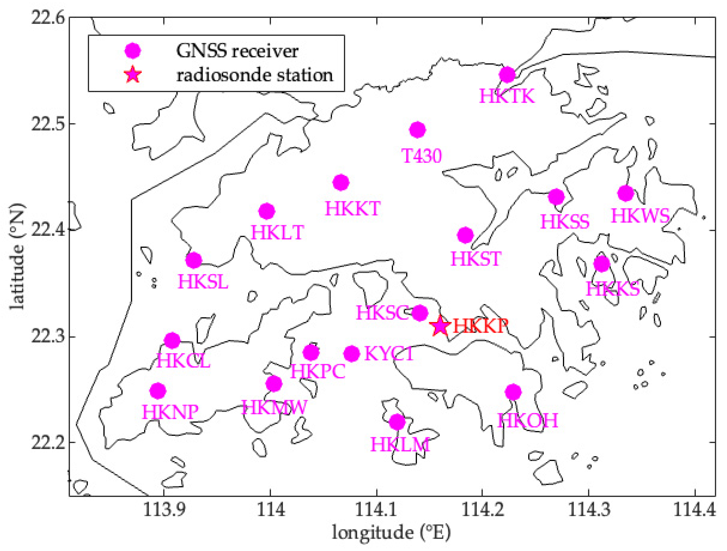
Figure 1. The geographical distribution of the 17 GNSS stations and the King’s Park radiosonde station in Hong Kong, China.
Remotesensing 14 05656 g001
Figure 2. The location of the selected 17 GNSS stations (magenta dots) and the radiosonde station (red pentagram) in the floor plan (a) and cutaway view (b) of the tomographic grid. The dashed line is the grid line of the tomographic voxel.
Remotesensing 14 05656 g002
Figure 3. The daily RE of the WVD resulting from the four tomographic schemes at each of the 10 tomographic layers during 2019.
Remotesensing 14 05656 g003
Figure 4. The monthly biases (a) and RMSEs (b) of WVDs resulting from the four schemes at each of the 10 tomographic layers during 2019. The x-axises of the upper and bottom panes are the bias (g/m3) and RMSE (g/m3), respectively; their y-axises are the same for the tomographic layers (1–10). The subfigures of the two panes from the left to the right are the results of months 1–12, and the title of each month is shown in the title of the subfigure of the upper pane (note: the x-axis range of the red box is different from the other x-axis ranges in the same pane).
Remotesensing 14 05656 g004
Figure 5. The skill score of the monthly RMSEs of SCH4 relative to SCH1, SCH2, and SCH3 at each of the 10 tomographic layers in each month during 2019.
Remotesensing 14 05656 g005
Figure 6. The annual biases (a) and RMSEs (b) of WVDs resulting from the four tomographic schemes at each of the 10 tomographic layers during 2019.
Remotesensing 14 05656 g006
Table 1. Four tomographic schemes employing two different vertical constraints with different parameters, i.e., SCH1, SCH2, and SCH3 with the traditional vertical constraint using different H parameter values and SCH4 with the new vertical constraint.
SchemeVertical ConstraintType of Parameter
SCH1 ρ w j = ρ w i e h j h i H H m e a n
SCH2 H f 1
SCH3 H r e a l t i m e
SCH4 ρ w j = ρ w i IRPWV h j , r IRPWV h i , r IRPWV h , r
1 H f = a H 0 + a H 1 cos ( doy · w ) + b H 1 sin ( doy · w ) + a H 2 cos ( doy · 2 w ) + b H 2 sin ( doy · 2 w ) .
Table 2. The statistical proportion of daily RE (%) (RE < 30% and RE > 50%) of WVD resulted from the four tomographic schemes at each of the 10 tomographic layers during 2019. Note that for the RE > 50% case, because the values of the statistical proportions at tomographic layers 1 and 2 are small, the values with one decimal place were adopted, as shown in the blue underline.
Tomographic Layer (km)RE < 30%RE > 50%
SCH1SCH2SCH3SCH4SCH1SCH2SCH3SCH4
1 (0–0.6)868599942.31.90.01.6
2 (0.6–1.2)857794960.81.50.10.6
3 (1.2–1.8)757578922222
4 (1.8–2.4)757576865555
5 (2.4–3)7071707412121114
6 (3–4)6363666426282425
7 (4–5)5251565538413633
8 (5–6)4139444548524538
9 (6–8)2319213268736947
10 (8–10)14992179868257
Publisher’s Note: MDPI stays neutral with regard to jurisdictional claims in published maps and institutional affiliations.