Article

Globally Scalable Approach to Estimate Net Ecosystem Exchange Based on Remote Sensing, Meteorological Data, and Direct Measurements of Eddy Covariance Sites

1
Carbonspace Ltd., D04H1F3 Dublin, Ireland
2
German Climate Computing Center (DKRZ), 20146 Hamburg, Germany
3
Technology Sector, Federal University of Paraná, Curitiba 80060, Brazil
4
LI-COR Biosciences, Daugherty Water for Food Global Institute, University of Nebraska-Lincoln, Lincoln, NE 68588, USA
*
Author to whom correspondence should be addressed.
Remote Sens. 2022, 14(21), 5529; https://doi.org/10.3390/rs14215529
Submission received: 16 September 2022 / Revised: 26 October 2022 / Accepted: 27 October 2022 / Published: 2 November 2022

Abstract

:
Despite a rapid development of Nature-Based Solutions (NBS) for carbon removal in recent years, the methods for evaluating NBS still have certain gaps. We propose an approach based on a combination of remote sensing data and meteorological variables to reconstruct the spatiotemporal variation of net ecosystem exchange from eddy-covariance stations. A Lagrangian particle dispersion model was used for upscaling satellite images and flux towers. We trained data-driven models based on kernel methods separately for each selected land-cover class. The results suggest that the proposed approach to quantifying carbon exchange on a medium-to-large scale by blending eddy covariance flux data with moderate resolution satellite and weather data provides a set of key advantages over previously deployed methods: (1) scalability, achieved via the validation design based on a separate set of eddy covariance stations; (2) high spatial and temporal resolution thanks to the use of Landsat imagery; and (3) robust and accurate predictions due to improved data quality control, advanced machine learning techniques, and rigorous validation. The machine learning models yielded high cross-validation results. Stratification that uses separate Fluxnet stations for each fold of validation ensures that the models are accurate across the area covered by the Fluxnet sites. Overall, we present here a globally scaled technology for the land sector based on high resolution remote sensing imagery, meteorological variables, and direct carbon flux measurements of eddy covariance flux stations.

1. Introduction

Nature-based solutions (NBS) are increasingly recognized as an essential tool in combating global warming as they remove greenhouse gases (GHG) from the atmosphere [1], reduce GHG emissions through sustainable land use practices, and store carbon in the soil and biomass [2]. While NBS are becoming quite advanced and continuously going through significant developments, the methods for accurately quantifying their resulting benefits are still lagging [3]. A vast majority of the existing projects use biometric soil or tree survey data to estimate carbon stock changes [4]. These methods provide solid estimates of the sequestered carbon but come with multiple important limitations. They typically describe either soil layer or partial canopy layer (e.g., above ground), with time resolution limited to multiple months and years and spatial resolution limited to a particular plot where such measurements have been performed. As a result of such limitations, these methods may not be best suited for large-scale ongoing NBS quantification [2]. Moreover, the measurements required by these methods for a meaningful time-resolved, large-scale assessment are expensive and unaffordable for most users.
A pure modeling approach employing either Earth system models or terrestrial biosphere models has been used as an alternative to direct measurements on a large scale [5,6], but the spatial resolution of these models is too coarse, while the uncertainty remains high due to their inability to respond timely to actual changes in the ecosystem. Likewise, satellites that measure carbon dioxide (CO2) concentrations and are used in inverse modeling to map GHG emission and sequestration [7,8] have coarse spatial resolution and hence can hardly be used for NBS assessment at the farm or forest stand level. Optical, radar, and lidar satellites provide a scalable solution for mapping soil carbon [9] and carbon fluxes at a much finer spatial resolution [10,11] and do have the potential to help large-scale space- and time-resolved NBS assessments if anchored in accurate ground measurements. The current remote-sensing-based studies typically use allometric/biometric data for machine learning (ML) model training [2]. The amount of ground data required for capturing the landscape heterogeneity and temporal variation is challenging to sustain and scale. The models thus inherit the disadvantages of the biometric measurements.
There is, however, another potential solution that combines many advantages of the above methods while overcoming some of their limitations and can result in a high spatial resolution, scalability to the regional level and practical affordability. This can be achieved by blending the direct highly time-resolved small-scale observations from the numerous eddy covariance flux towers [2] and the less direct but large-scale remote sensing methods. Considerable efforts have been made in this area lately to improve the quantification of the spatiotemporal CO2 patterns, employing multiple different approaches vs. existing estimates to help resolve the majority of issues with current carbon accounting methods in the land sector. For example, [12] evaluate how seven light-use-efficiency (LUE) models captured the spatiotemporal gross primary productivity (GPP) variations from the LaThuile FLUXNET dataset. This study used data from 157 eddy covariance (EC) towers located in the six major terrestrial biomes (evergreen broadleaf forest (EBF), deciduous broadleaf forest (DBF), mixed forest (MF), evergreen needle leaf forest (ENF), shrubland (SHR), and grassland (GRA)). None of the seven models matched well with estimated GPP based on overall EC measurements. The models explained 41–57% GPP variations in the study sites. Reference [13] evaluated four LUE models for GPP estimation and compared them with data obtained by EC in 51 sites with diverse vegetation types. The average daily R 2 for all models and all sites was about 66%. Reference [14] used three different models to estimate GPP in a local deciduous forest in the US in combination with flux measurements and remote sensing data. Comparisons were made yearly, but on average, the correlation coefficient was much better, at 0.91. Reference [15] used two enhanced vegetation index (EVI)-based models to estimate the GPP in 15 sites across the USA. The model’s results vary according to the vegetation; in some cases, coefficients of determination can vary from 0.27 up to 0.94 for specific sites. Using remote sensing data, disturbance information, and a support vector regression model, [16] upscaled the CO2 fluxes from a network of 21 EC towers to estimate the regional-scale Alaskan CO2 budget from 2000 to 2011 and compared the results with an inverse model. The predicted values were consistent with the field observations ( R 2 = 0.79 for NEE) and the magnitude of the inverse model. However, the interannual variations of the results achieved by the remote-sensing-based model and those of the inverse model were inconsistent and therefore require additional validation. Reference [17] used three remote sensing data-driven models to evaluate and understand GPP estimations in 119 EC sites in the northern hemisphere. Considering all the study sites, the mean R 2 was 0.63. However, the values can vary significantly depending on the model used and the vegetation, and in some cases, they can reach 0.78. Usually, the highest values were found for deciduous broadleaf and mixed forest. Reference [18] mapped the soil organic carbon (SOC) in Italy using ground observations and ancillary remote sensing data. Compared with all observations, the geographically weighted regression using MODIS normalized difference vegetation index (NDVI) obtained an R 2 of 0.45 for SOC. Reference [19] conducted comprehensive work generalizing and mapping NEE, GPP, and respiration data for all types of classification as a collaborative FLUXCOM initiative. The overall coefficients of determination for GPP and respiration were more than 0.71 and 0.64, respectively, while about 0.48 for NEE.
As seen in the examples above, despite the significant advances in the use of remote sensing for CO2 flux estimations, the results point to mixed success and lack of consistency, so there is room for major improvements. The key areas of such improvements include increasing spatial resolution, capturing temporal variability, improving the data quality (primarily by reducing uncertainties and increasing consistency) and developing better algorithms to enable the simultaneous use of multiple relevant parameters and different spatial and temporal scales. In order to achieve such improvements, we propose to rely on the significant advances which have been made in recent years in the fields of machine learning, artificial intelligence, and neural networks to extract patterns and insights from remote sensing data, processing large volumes of remotely sensed data with minor human interference [20]. Here, we present the successful use of one such approach for globally scaled remote-sensing-based carbon accounting models anchored by the direct carbon flux measurements using eddy covariance flux stations. We use input data on the net ecosystem exchange (NEE, [21,22,23,24]) as targets for the training process and then combine the remote sensing and meteorological variables [19] as predictors to reproduce variations of NEE on a daily and monthly scale to demonstrate the increased predictive power of the proposed approach over more traditional methods.
An overarching goal of this work is to bridge the domains of science and technology by integrating multi-scale remote sensing and eddy covariance measurements to support projects aimed at avoiding GHG emissions or to remove CO2 from the atmosphere. For this purpose, we target the following methodological improvements: (1) increasing spatial resolution, (2) capturing temporal variability, (3) improving the data quality (primarily by reducing uncertainties and increasing consistency), and (4) developing better algorithms to enable the simultaneous use of multiple relevant parameters and different spatial and temporal scales.

2. Data and Methods

2.1. Data

2.1.1. Eddy Covariance Data

The eddy covariance method is a standard method to directly measure fluxes between ecosystems and the atmosphere by computing the covariance between the vertical wind velocity and the entity of interest [21,25,26]. Such measurements are made routinely on all continents [27,28,29], with many sites linked across a global network called FLUXNET, dispersed across the world’s climate zones and representative biomes [29,30,31,32,33]. FLUXNET teams standardize the data format, perform uniform quality checks, and use highly vetted gap-filling and flux partitioning, with the newest product version being the FLUXNET2015 dataset (we used data for 2000–2014), which includes over 212 sites [32] (see Figure 1).
We used data from 171 Tier 1 sites with a data policy consistent with the Attribution 4.0 International (CC-BY-4.0) data usage license. Daily net ecosystem exchange (NEE) was filtered using a variable friction velocity threshold for each year and quality flags indicating the measured and good quality percentage (data higher than 0.8 were used, indicating percentage of measured and good quality gap-fill data). The following land-cover classes based on the International Geosphere-Biosphere Programme (IGBP) classification were used: cropland (CRO); grassland (GRA), which includes grasslands, closed shrublands (CSH), and open shrublands (OSH) [34]; evergreen needleleaf forest (ENF); deciduous broadleaf forest (DBF); evergreen broadleaf forest (EBF); mixed forest (MF); wetland (WET); and savannas and woody savannas (SAV).

2.1.2. Remote Sensing Data

We used Landsat surface reflectance (SR) and land surface temperature (LST) as well as a number of indices derived from the former as the main predicting features for our machine learning model. Landsat 5, 7, and 8 (TM, ETM+, and OLI respectively) cover our study period and have a 30 m spatial resolution. USGS provides open access to their Landsat Collection 2 Level-2 Science Products (L2SP) through Amazon s3 cloud service. L2SP data are geometrically and atmospherically corrected using the LEDAPS algorithm for TM and ETM+ and LaSRC for OLI imagery and thus prepared for scientific analyses. USGS Landsat was accessed from https://registry.opendata.aws/usgs-landsat (accessed on 1 February 2022).
We filtered out imagery with cloud cover above 75% of a scene. To ensure consistently high data quality, we masked out all possible artifacts as marked in the quality assessment bands provided with the product. We also left out high- to low-confidence clouds and cloud shadows detected by the CFMask algorithm [35].
We utilized SR from three visible, near-infrared (NIR), and short-wave infrared (SWIR 1 and SWIR 2) spectral bands (bands 1–5 and 7 for TM and ETM+; and 2–7 for OLI). These bands are well-suited for assessing vegetation and soil state and, consequently, together with LST, can serve as accurate predictors of NEE.
In addition, we selected two spectral indices and two tasseled-cap components [36] to map proxy land surface parameters to predict NEE better. Soil-adjusted vegetation index (SAVI) and tasseled-cap greenness (TCG) reflect vegetation intensity and chlorophyll content. In contrast, normalized-difference moisture index (NDMI), normalized difference vegetation index (NDVI), enhanced vegetation index (EVI), and tasseled-cap wetness (TCW) reflect moisture content in vegetation in our areas of interest [37,38].
T C G = 0.1603 · b l u e + 0.2819 · g r e e n 0.4934 · r e d + 0.7940 · N I R 0.0002 · S W I R 0.1446 · S W I R 2
T C W = 0.0315 · b l u e + 0.2021 · g r e e n + 0.3102 · r e d + 0.1594 · N I R 0.6806 · S W I R 0.6109 · S W I R 2
N D M I = N I R S W I R N I R + S W I R
N D V I = N I R r e d N I R + r e d
S A V I = N I R r e d N I R + r e d + 0.5 · 1.5
E V I = 2.5 · N I R r e d N I R + 6 · r e d 7.5 · g r e e n + 1
where b l u e , g r e e n , r e d , N I R , S W I R , S W I R 2 are Landsat spectral bands of the corresponding wavelengths.

2.1.3. Meteorological Data

In addition to the remotely sensed data characterizing the vegetation cover, the performance of NEE is influenced by weather parameters such as temperature, dew-point temperature, solar radiation, and precipitation. The global dataset AgERA5 was chosen as the source of this data [39].
This service is based initially on hourly European Centre for Medium-Range Weather Forecasts Reanalysis version 5 (ECMWF ERA5) data at the surface level, which are available at 30-km spatial resolution (about 0.28125°). Data were processed to daily temporal resolution by summing or averaging depending on a particular parameter and corrected to a more refined surface description at a 0.1° spatial resolution. Aggregated data follow a local time zone definition and include several major agronomic parameters. The correction to the 0.1° grid was performed by applying grid and variable-specific regression equations to an ERA5 dataset interpolated at a 0.1° grid. The equations were trained on operational ECMWF’s high-resolution atmospheric model (HRES) data at a 0.1° resolution.
The following set of parameters was chosen for our purposes: 24 h mean of 2 m air temperature ( T e m p e r a t u r e A i r ), 24 h mean dew-point temperature ( D e w P o i n t ), precipitation flux (sum of total precipitation per day, P r e c i p i t a t i o n F l u x ), and surface solar radiation downwards (sum of solar radiation per day, S o l a r ). A description of the additional meteorological features generated and used in this work is provided in Section 2.2.2.

2.2. Simulation Experiment

The eddy covariance method measures fluxes integrated over an upwind area of a specific size, known as a footprint [40,41]. The size of this area depends significantly on wind speed and direction. The NEE measurements from stations have a half-hour temporal resolution, which means that the station is sensitive to the area around at a distance that air mass has passed upstream during a specific half-hour. The linear scale of such an area may range from hundreds of meters to several kilometers.
Thus, in the case of 30 m resolution remote sensing data, we cannot directly associate the surface reflectance value in a band’s pixel (or calculated index) with the station inside and NEE estimation on this station for the specific date. In order to do so, we need to calculate the relevant weighted footprint [42,43] of the impact area around the station for the corresponding time scale (daily in our case, see Figure 2). To calculate this footprint, we used a meteorological model which can reproduce transport processes on a local scale depending on weather conditions on a given day. For this purpose, we used the Lagrangian particle dispersion model (LPDM) FLEXPART. We weighted six Landsat-derived spectral bands and indices and integrated them by a footprint probability density function estimated using the FLEXPART model in backward mode. There is no need to do such a calculation for meteorological features, as their spatial resolution is coarser (linear size of gridcell about 9–10 km or 100 km2).

2.2.1. Footprint Calculation with LPDM

We used the Lagrangian particle dispersion models (LPDM) FLEXPART [44,45] to estimate the footprint of Fluxnet stations. In Lagrangian models, individual particle trajectories (representing air parcel transport) are calculated following a predetermined atmospheric wind field and other meteorological variables. LPDMs can run forward (source to a receptor) or backward (receptor to source) modes.
We used the FLEXPART version 8.2, which utilizes National Center for Environmental Prediction Final (NCEP FNL) operational global meteorological data on a regular latitude–longitude horizontal grid with 0.25–1.0 degree spatial resolution on hybrid sigma-pressure vertical levels and temporal resolution of 3–6 h. The model output grid has a spatial resolution on a latitude–longitude grid with 0.002 degrees (about 150–200 m), and the smoother result, the model synchronization time step, was 15 s.
We ran the model in a backward mode to obtain the weighted footprint for a specific station, setting station parameters such as location coordinates and above-ground height as receptor position. The duration of trajectories was selected corresponding to the original EC system time scale, which is 30 min for which the residence time is calculated. Residence time is a regular output parameter of FLEXPART model in the backward mode. This model setup was run six times a day (i.e., every 4 h) for every station for every date where satellite images were available to obtain a daily footprint.
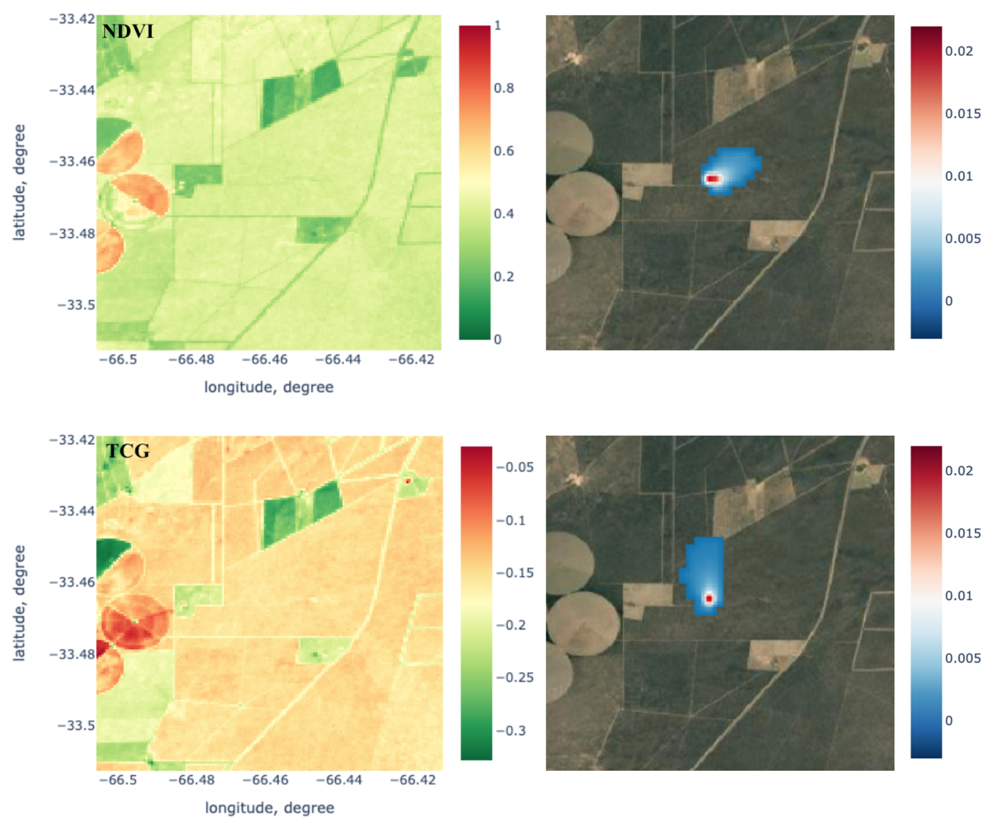
One of the regular output parameters of the FLEXPART model in backward mode is residence time, which is measured in seconds. That gives an understanding of how long one particle (effective air parcels), or group of particles, has “lived” in a particular grid cell, which allows us to evaluate the receptor’s sensitivity to the surface grid cells. Thus, the resulting residence time map can be interpreted as a weighting function (see Figure 3 right panels), which we need to rely on when processing the remote sensing data.

2.2.2. Feature Generation and Data Augmentation

We selected the resampled, weighted, and aggregated SR and the LST values from the Landsat bands, indices calculated from these bands, and the set of meteorological parameters taken from the reanalysis AgERA5 as predictors of a regression model to predict daily NEE, which is a product from Fluxnet stations (see Section 2.1.1).
In this study, a set of additional features was created to increase the flexibility of the regression model and expand the interactions between the base predictive features and the target variable. First, all possible ratios were created between 6 Landsat bands and LST. Thus, we have five ratios for blue band, four ratios for green band, three ratios for red band, two ratios for NIR, and one ratio for SWIR1 (e.g., blue/green, blue/red, blue/NIR, 15 features in total). When we computed vice versa, we obtained five ratios for SWIR2, four ratios for SWIR1, three ratios for NIR, two ratios for red, and one ratio for green (e.g., green/blue, red/blue, NIR/blue, 15 features in total). Another set of features is a list of ratios between bands and LST (blue/LST, green/LST etc. 12 features in total). As a result, 42 features were added to the predictive dataset. Second, from meteorological variables such as solar radiation, 2 m air temperature, and precipitation flux, additional features were also created. For solar radiation, cumulative and mean radiation over five different periods were calculated: four days, one week, two weeks, three weeks, and four weeks (ten features as a result), which may show delayed phenological effects on sub-seasonal and seasonal scales. The same set of parameters was prepared for 2 m air temperature. For precipitation flux, cumulative precipitation for the last one, two, three, four, and five days was calculated (five features). Thus, 25 more features were added to the base predictive features. In total, 87 features were prepared for further training.
Another issue in the dataset collection process is the availability of clear-sky observations from the Landsat constellation. After merging the dates with available satellite images and good quality NEE observations, fewer training points remain, mainly due to the images’ cloud cover and other artifacts. We decided to apply training sample augmentation techniques to solve this problem.
The procedure for increasing the training sample is based on the assumption that the surface reflectance on the day of satellite measurements and the neighboring days will be similar given similar weather conditions. Weather variables, i.e., precipitation, air temperature, short-wave, and incoming long-wave radiation, were determined using data from local meteorological measurements at each eddy-covariance station. From these four parameters, a weather profile was generated for the whole time series of daily NEE estimations, which was then compared with a similar profile on the day of satellite observations. If the R 2 value was greater than 0.9, it was assumed that the day had similar weather conditions, and images of the original day could be applied to such a day. As a result, we used the same Landsat scenes for remote sensing parameters at augmented days from the original observation date, while applying the weighted footprint function for that specific day. The time considered in this study was a week before the date of Landsat observation. As a result, the size of the training sample was increased by about a factor of 3.

2.2.3. Building Regression Model

We used Python as a programming language and performed the calculations on Amazon Web Services (AWS, Seattle, WA, USA). We processed 20,438 Landsat scenes for this study. Apart from satellite imagery processing, calculations associated with the feature selection process (from a few thousand features) were among the most computationally intensive.
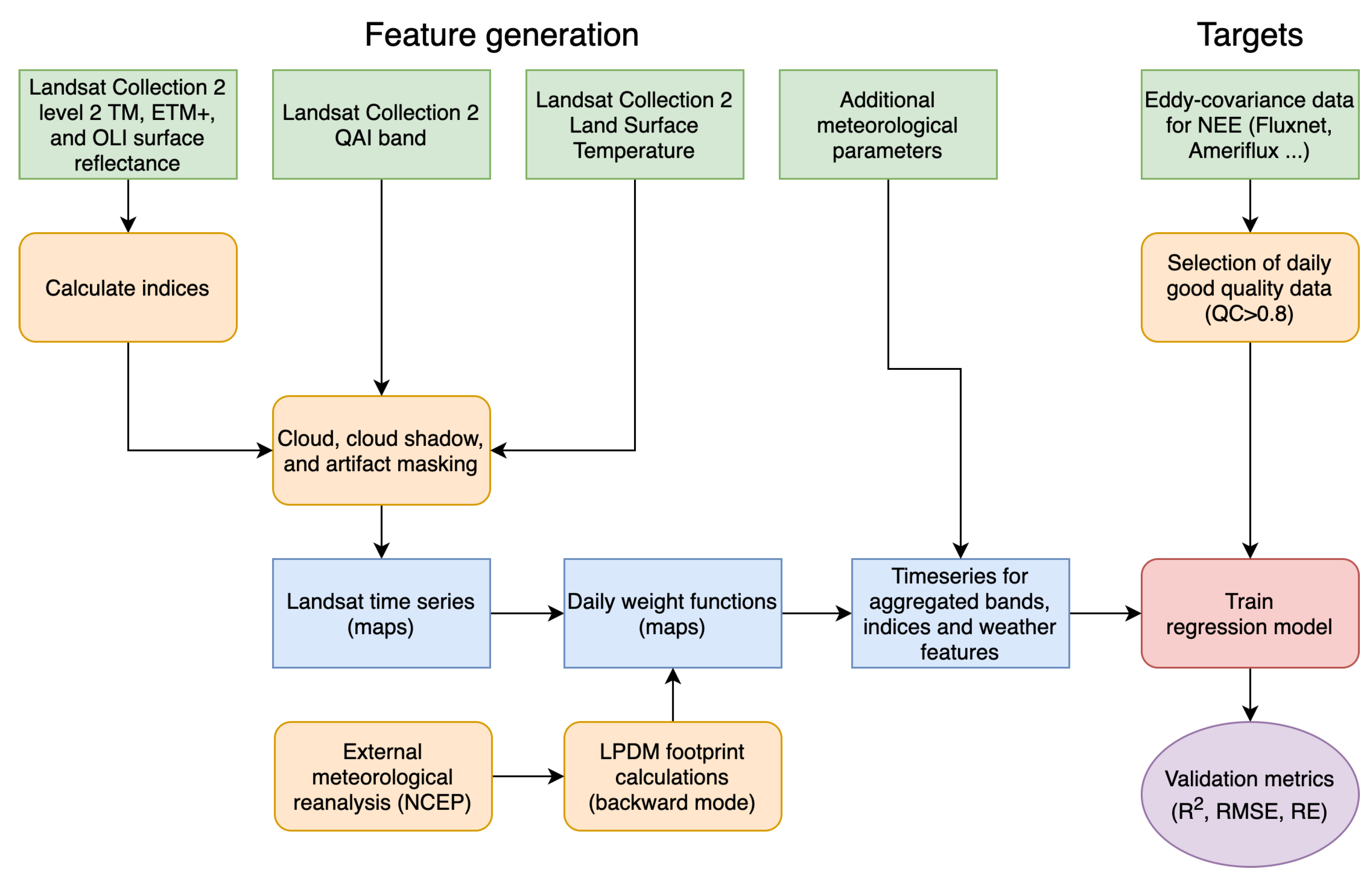
Figure 2 demonstrates the data flow for the dataset creation process. The formulas for calculating weighted parameter values and a regression model are as follows:
F w e i g h t e d j = i = 1 N w i F i j
N E E = H ( F w e i g h t e d 1 , F w e i g h t e d 2 , , F w e i g h t e d M )
where w i —weight value for the i-th grid cell (see Figure 3); F i j — value of j-th predictive feature for i-th grid cell; F w e i g h t e d j —weighted sum for j-th feature; NEE—eddy covariance data; N—number of grid cells; M—number of features; and H—non-linear operator.
Figure 3 shows an example of original features calculated from Landsat data and results of LPDM calculations of the footprint for the up-scaling process. The weighted sum for each parameter may be interpreted as the dot product of the feature and footprint map. To train the model, we match the resulting input dataset (Table 1) with eddy covariance data (Table 2).
We selected an algorithm based on the kernel method kernel ridge regression (KRR) [46,47]. This method is similar to the more widely known class of support vector machine (SVM) methods [48]. However, it uses a different loss function. The KRR method uses linear least squares with l2-norm regularization, meaning it has scale factor for squared feature coefficients as an additional term in the loss function. This allows for creating non-linear dependencies between the features according to the selected kernel and then searching for the optimal coefficients of these dependencies with control of the regularization process. The result of solving such a problem is a hyperplane in the multidimensional feature space that describes the dependencies of the target values on the selected features. This method works well with small datasets, which is the case in this study and is also faster than the original support vector regression (SVR).
KRR has three main hyperparameters: α —the regularization parameter of the model (the higher the value, the stronger the regularization); kernel—kernel interaction between the features included in the model (see Equations (9) and (10)); γ —internal kernel parameter (see Equations (9) and (10)).
k ( x , y ) = e γ x y 1
k ( x , y ) = e γ x y 2
where e—exponent; x, y—input vectors; x y 1 —Manhattan distance between the input vectors; and x y 2 —Euclidean distance between the input vectors.
Another critical aspect of preparation is the feature selection process. As mentioned in Section 2.2.2, in addition to the primary remote sensing and weather parameters, 87 additional features in total were prepared. In addition, we used products between all meteorological and remote sensing features that led to a few thousand features.
For each IGBP class, a small set of features has to be selected to allow optimal prediction of NEE at the stations. The exact solution for finding the optimal combination of features can be obtained by a complete enumeration of all possible variants. The complexity of this approach is 2 n , where n is a number of features, so the approach becomes inapplicable for a large number of features. The utilities in the package machine learning extensions (Mlxtend) [49] were used to select the features.
The selection process was divided into two stages. The first stage estimates mutual information for each feature in the list. A standard method from the scikit-learn library was used [50], which allows us to reduce the number of features to select. The second step is a sequential selection of features in the forward mode. That means the model starts to learn from one feature and sequentially adds features to improve the quality of the model. As a result of this selection, the feature sets for each IGBP class have been generated, as shown in Table 3.
Model training and hyperparameters tuning processes were based on N-fold cross-validation. In our case, N equals 3, 5, or 7 depending on the size of the available dataset per IGBP class. The original dataset was divided into N nearly same-sized folds with a unique set of Fluxnet sites inside. Then, the model was trained on N 1 folds and validated on the remaining fold after the procedure was repeated N times with different combinations of folds. Each fold contains a unique set of stations without overlapping with other folds [51], which ensures spatial scalability. Thus, N times independent validation was performed on the sets of stations that were not involved in the training of the model, which ensures spatial scalability of the model predictions. Similarly to [19], hyperparameters for each N fold were tuned separately for a fixed set of features. As a result, we have not just one model per land cover but an ensemble of models with their respective metrics trained on a different dataset configuration.

2.2.4. Metrics for Accuracy Assessment

Several standard metrics were used to assess the level of accuracy for the trained NEE estimation model: mean absolute error (MAE), root mean squared error (RMSE), coefficient of determination ( R 2 ), and relative error (RE).
R M S E = 1 N i = 1 N ( y i t y i ) 2
R 2 = 1 i = 1 N ( y i t y i ) 2 i = 1 N ( y i t y ¯ ) 2
R E = 1 N i = 1 N | y i t y i | 1 N i = 1 N | y i t y ¯ |
where N is the number of observation points to estimate; y i t and y i are the i-th true and modeled NEE value respectively; and y ¯ is the mean NEE value.

3. Results

As a result of N-fold cross-validation for each land cover (Section 2.2.3), we received an ensemble of N different models trained on different independent datasets with the same inputs. Thus, we can use the mean value over the ensemble as a prediction.
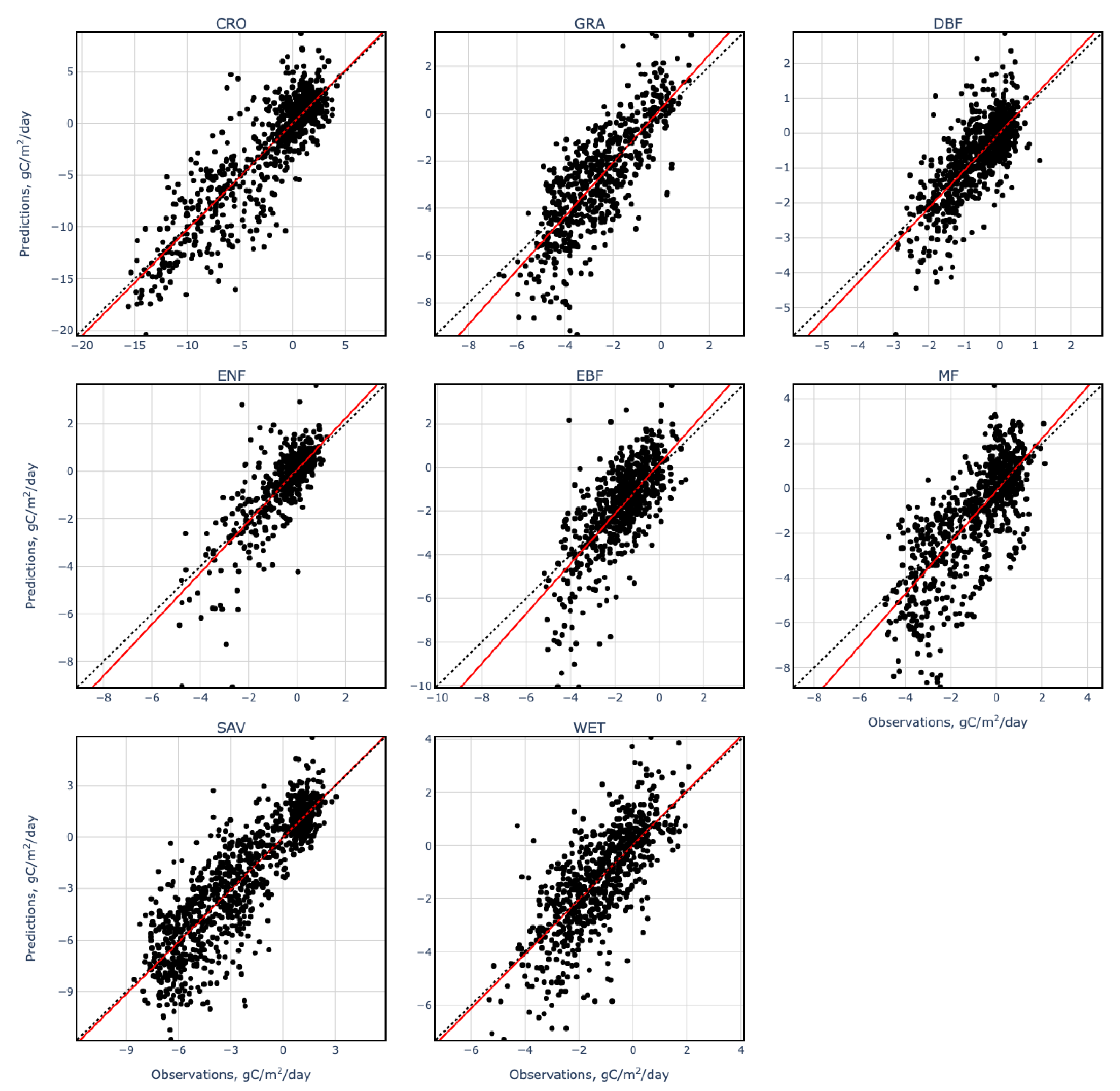
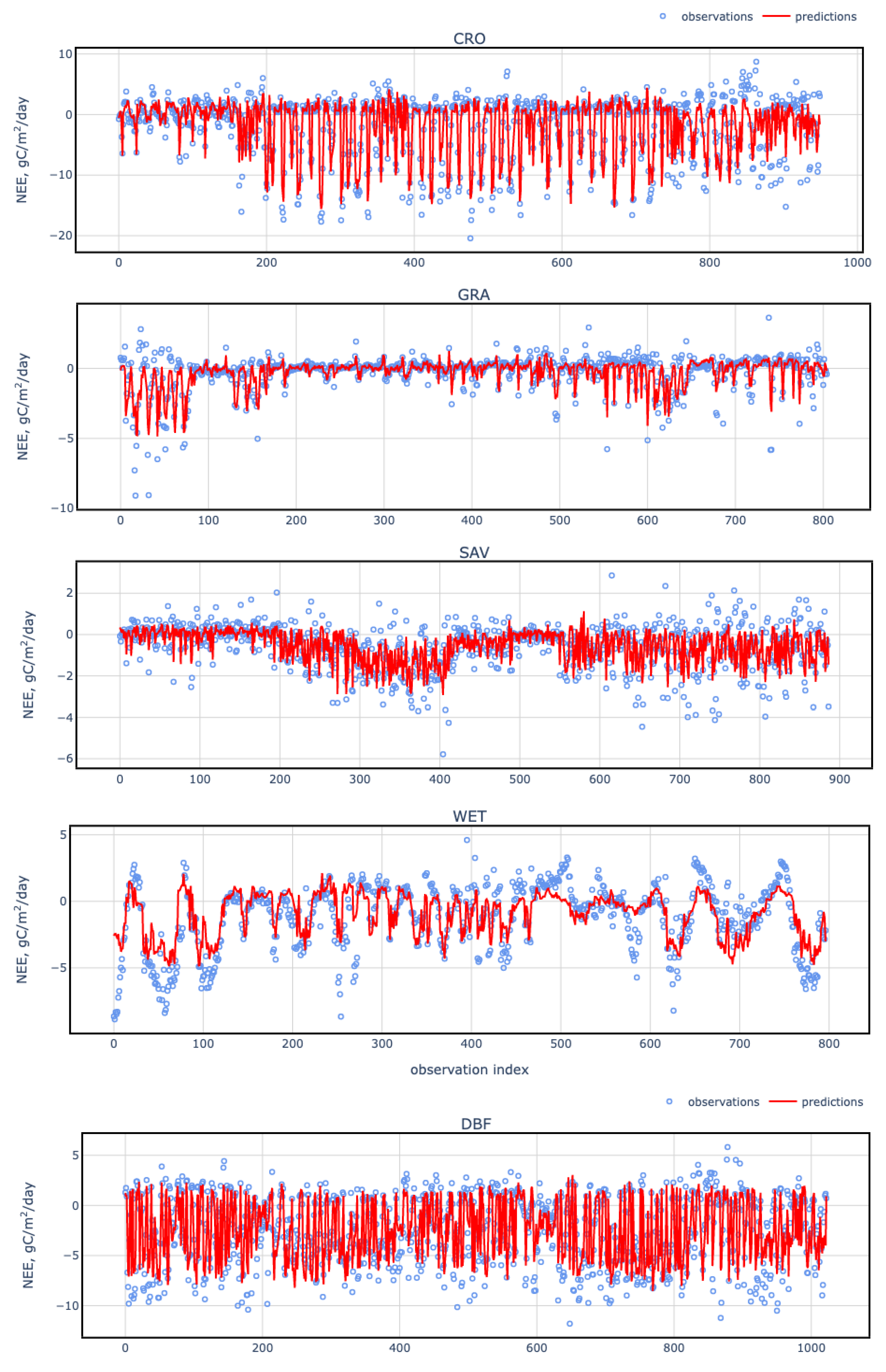
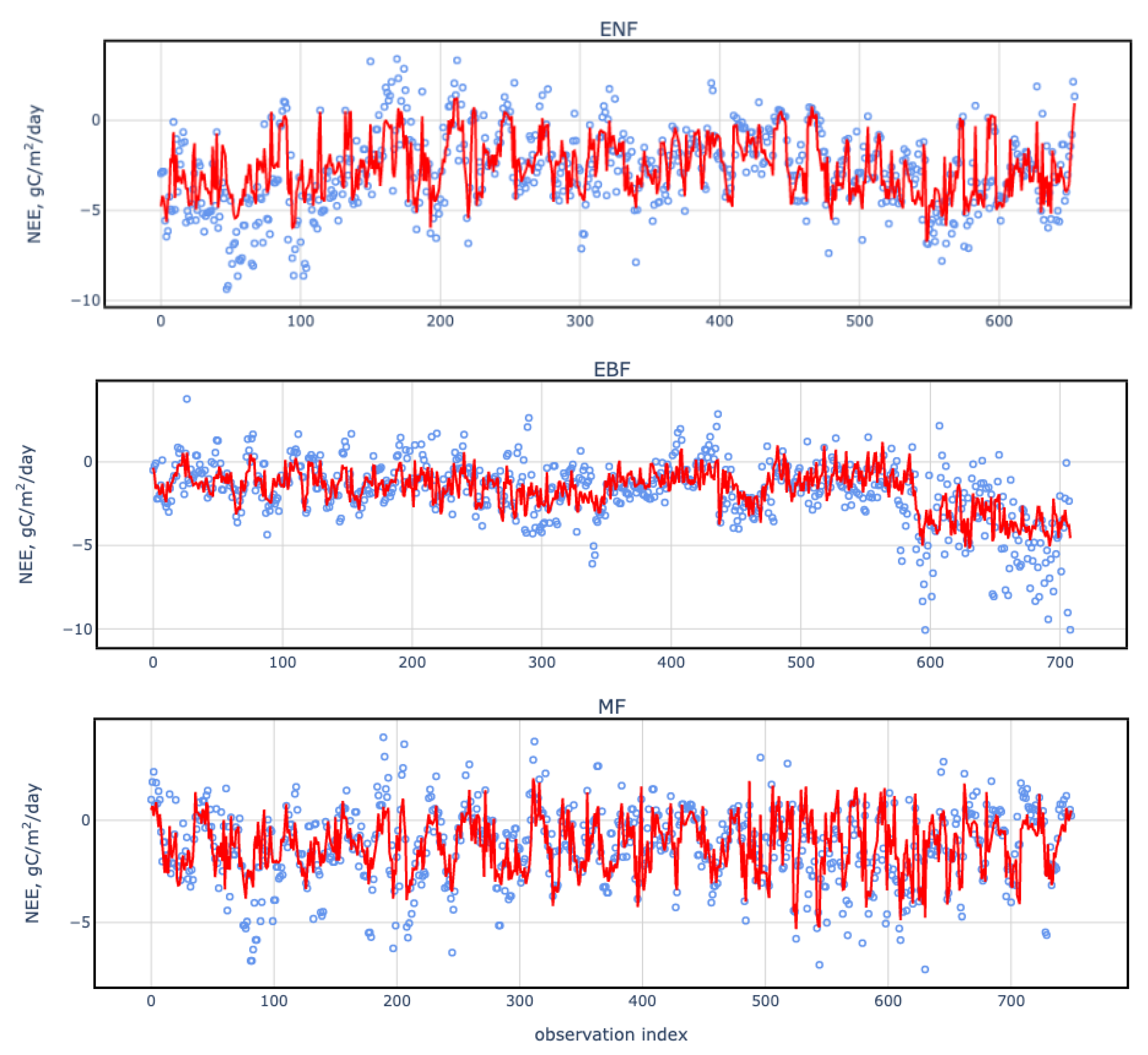
First, selected metrics were applied to estimate the model’s accuracy by reproducing the original daily NEE values and then used to estimate the accuracy of the predicted NEE behavior. The results of the training and cross-validation experiments based on independent stations are presented in Table 4. The trained models can adequately reproduce the behavior of NEE at stations with different land cover (overall mean across land-cover NEE, R 2 > 0.6 with a range of 0.42 to 0.76). The lowest predicted values are for EBFs because such forests are mostly located in the tropics, where there are few Fluxnet stations, and there could be problems with cloud conditions during some seasons. The largest variation in error (standard deviation) is observed for CRO, possibly due to the difference in crop types and significant local anthropogenic influence on specific fields. An increase or decrease in NEE can be explained by the state of the biomass and the influence of agricultural management. Comparisons of observed values and predicted values are shown in Figure 4 and Figure 5.
To compare monthly NEE, additional daily footprint calculations similar to Section 2.2.1 were carried out. In this case, the calculation period of one week before and one week after the available satellite images were selected. Usually, periods of 8 days are used [19,34], but in our case, we decided to use a similar averaging backward and forwards. Furthermore, remote sensing data from the original image was used for the additional dates, but with meteorological variables and weighting functions corresponding to the actual date. Monthly model NEE data were then calculated for those months where it was possible to predict more or equal to 2/3 days of the month. The resulting monthly NEE was compared with monthly NEE values from stations for which the quality flag was greater than or equal to 0.8. The results of the comparison are presented in Table 5.

4. Conclusions

There has been a drastic rise in NBS development in recent years [3]. Although the methods for evaluating NBS are advancing, there are still certain gaps that need to be addressed [2]. Previous studies found that most of the current methods for quantifying NBS benefits use biometric soil or tree survey data to estimate carbon stock changes. These methods do not enable seamless large-scale assessments, while associated regular measurements make the methods financially unsustainable for most players in the land sector. Modeling approaches based on Earth system models or terrestrial biosphere models, as well as inverse modeling based on CO2 concentrations data, have spatial resolution too coarse to be used locally. The current remote-sensing-based approaches mainly rely on allometric data as ground truth and therefore involve challenges with capturing landscape heterogeneity and temporal variation that negatively impact scalability. As the result of the analysis from the recent studies, it is fair to say that the approaches based on observations from eddy covariance towers and remote sensing are the best fit to enable affordable, high spatial resolution, globally scalable CO2 estimates. We analyzed the studies representing a vast amount of scientific efforts targeted on these approaches and identified the significant challenges. Here, we presented an improved approach to quantifying carbon fluxes by blending eddy covariance data with moderate resolution satellite data and weather data. Our method (1) is scalable due to the validation design based on a separate set of eddy covariance stations, (2) features a high spatial and temporal resolution of the Landsat data and set of meteorological variables, and (3) delivers robust and accurate predictions due to improved data quality control, advanced machine learning techniques, and rigorous validation.
Fluxnet towers are expected to estimate NEE values for homogeneous land covers that are stable over time. Therefore, in order to apply our method the regions should be thoroughly controlled for these parameters. In addition, models can only be applied to the areas with known land cover. Application to areas with different land cover may skew the results significantly. At the same time, the eddy covariance system captures the net ecosystem exchange, which accounts for total CO2 fluxes, including those related to the heterotrophic respiration process. So if the AI remote sensing model was trained with EC NEE, it consequently accounts for heterotrophic respiration.
In terms of global coverage, it is true that the sites we use may not be representative for all possible climate zones. However, since we use several validation folds that are blindly compiled (we do not know which station from which region is in which fold), we can assume that the regression we have constructed (ensemble of models) may be able to describe the underlying behavior processes for NEE. Such estimates then can be applied globally. A exact conclusion can be drawn using new EC data from independent sources and other climate zones.
Further in the Discussion, we suggest the key reasons for these improvements and also list our opinion on the current limitations of the proposed approach. Our methodology employed eddy covariance data from the Fluxnet network. Since the network has a standardized methodology for data acquisition and processing, we collected a robust and consistent training dataset, typically unavailable for more traditional carbon accounting methods based on biomass and soil sampling. The availability of a large amount of consistent and uniform data allowed for setting a fairly conservative threshold of 80% for the NEE data coverage and resulted in substantially reduced noise. On the remote sensing side of the approach, the Landsat archive provided a consistent and robust set of data with great temporal depth and spatial resolution. The FLEXPART model was instrumental in mapping the area that contributed to the NEE values captured by flux stations, helping to match these with remote sensing products better to account for landscape heterogeneity. Utilization of the KRR and its parameterization tailored to the goals of this study, and strict feature selection, enabled high prediction accuracy.
Still, the metrics of our regression estimators were not uniform and varied across the land-cover classes. The R 2 for the DBF was the highest, likely due to clear seasonality patterns and relatively low heterogeneity within the class. The same metric for the EBF class was the lowest, likely due to other carbon exchange process drivers and lower data availability due to high cloud cover in tropical regions.
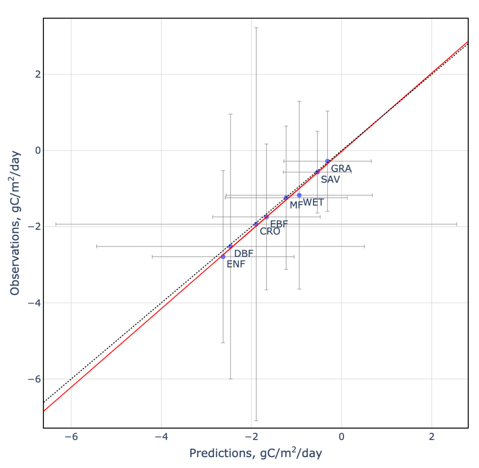
Current results are presented for each land-cover class globally, providing visibility on the unified, scalable calculation approaches and the global accuracy baselines for various land covers (Figure 6). Overall, the achieved accuracy was in line with similar studies but outperformed most of those targeting global geographical coverage (overall land cover cross-validation R 2 = 0.73, RMSE = 1.53 gC/m2/day). Daily data accuracy has the R 2 range between 0.42 for EBF and 0.76 for DBF (monthly data accuracy is between 0.6 for GRA and 0.84 for DBF). The models have better accuracy in those parts of the world where the number of stations is higher and, conversely, slightly worse accuracy in areas of lower station density.
To resolve or minimize these deficiencies and improve accuracy for specific cases or regions, the current system allows additional training (not a local re-training) in the presence of the additional local flux observations, as suggested by [2]. Another way to improve the confidence of model data is to add other multispectral, hyperspectral, and radar satellite products, e.g., Sentinel-1, 2, or EnMap. It is expected that these new data streams can improve the accuracy of the daily data slightly but can contribute significantly to the monthly and annual data improvement.
Finally, since in this study we have trained N independent models for each land cover (where N = 3, 5, 7). In the future, it may be better to use ensemble predictions to allow additional characteristics such as mean, median, and standard deviation. These and other activities are currently in development but not advanced enough to be included in this manuscript.
Given the urgent need to decarbonize the atmosphere and the critical role of NBS in doing so, a fusion approach of eddy covariance and remote sensing data proved to be an efficient and cost-effective solution for quantifying these efforts. We hope our methods could contribute to mitigating global climate change in a cost-effective and transparent way.

Author Contributions

Conceptualization, R.Z. and A.D.; methodology, R.Z. and A.D.; software, R.Z. and A.D.; validation R.Z.; writing—original draft preparation, R.Z., A.D., A.L.D.d.S. and O.D.; writing—review and editing, A.D., O.D. and G.B. All authors have read and agreed to the published version of the manuscript.

Funding

This research received no external funding.

Data Availability Statement

Not applicable.

Acknowledgments

We thank Igor Susman (Chief Technical Officer at CarbonSpace Ltd.) and the IT team of CarbonSpace for developing infrastructure and supporting our calculations. We thank Ray Mercedes (Head of Innovation at CarbonSpace Ltd.) for extremely valuable suggestions, contributions to the paper, and overall support of the work. We thank Andrey Samodin (Chief Marketing Officer at CarbonSpace Ltd.) for significant contribution to the draft preparation. We would like to thank the anonymous reviewers for their valuable comments and suggestions.

Conflicts of Interest

The authors declare no conflict of interest.

Appendix A. Input Data Description

Table A1 contains a description of eddy covariance study sites from Fluxnet (2000–2014) involved in training process (84 stations left after data filtering). The total amount of data for each land cover was as follows: CRO (948 data points), GRA (803 data points), DBF (1023 data points), EBF (709 data points), ENF (675 data points), MF (750 data points), WET (801 data points), and SAV (887 data points).
Table A1. List of eddy covariance sites after quality control procedure.
Site CodeLatLonIGBPStart YearEnd Year
BE-Lon50.55164.7462CRO20042014
CH-Oe247.28647.7337CRO20042014
DE-Geb51.099710.9146CRO20012014
DE-Kli50.893113.5224CRO20042014
FR-Gri48.84421.9519CRO20042014
IT-BCi40.523714.9574CRO20042014
IT-CA242.377212.026CRO20112014
US-ARM36.6058−97.4888CRO20032012
US-CRT41.6285−83.3471CRO20112013
US-Lin36.3566−119.0922CRO20092010
US-Ne141.1651−96.4766CRO20012013
US-Ne241.1649−96.4701CRO20012013
US-Ne341.1797−96.4397CRO20012013
US-Twt38.1087−121.6531CRO20092014
DE-Hai51.079210.4522DBF20002012
DE-Lnf51.328210.3678DBF20022012
DK-Sor55.485911.6446DBF20002014
FR-Fon48.47642.7801DBF20052014
IT-CA142.380412.0266DBF20112014
IT-CA342.3812.0222DBF20112014
IT-Col41.849413.5881DBF20002014
IT-Isp45.81268.6336DBF20132014
IT-PT145.20099.061DBF20022004
IT-Ro142.408111.93DBF20002008
IT-Ro242.390311.9209DBF20022012
US-Ha142.5378−72.1715DBF20002012
US-Oho41.5545−83.8438DBF20042013
US-UMB45.5598−84.7138DBF20002014
US-UMd45.5625−84.6975DBF20072014
US-WCr45.8059−90.0799DBF20002014
AU-Cum−33.6152150.7236EBF20122014
AU-Wac−37.4259145.1878EBF20052008
AU-Whr−36.6732145.0294EBF20112014
AU-Wom−37.4222144.0944EBF20102014
CN-Din23.1733112.5361EBF20032005
FR-Pue43.74133.5957EBF20002014
IT-Cpz41.705212.3761EBF20002009
CZ-BK149.502118.5369ENF20042014
DE-Obe50.786713.7213ENF20082014
DE-Tha50.962613.5651ENF20002014
IT-Ren46.586911.4337ENF20002013
IT-SRo43.727910.2844ENF20002012
US-Blo38.8953−120.6328ENF20002007
AU-DaP−14.0633131.3181GRA20072013
AU-Stp−17.1507133.3502GRA20082014
AU-TTE−22.287133.64GRA20122014
CH-Cha47.21028.4104GRA20052014
CH-Fru47.11588.5378GRA20052014
CH-Oe147.28587.7319GRA20022008
CN-Cng44.5934123.5092GRA20072010
ES-Amo36.8336−2.2523OSH20072012
ES-LJu36.9266−2.7521OSH20042013
US-AR136.4267−99.42GRA20092012
US-AR236.6358−99.5975GRA20092012
US-Goo34.2547−89.8735GRA20022006
US-Igreen41.8406−88.241GRA20042011
US-SRC31.9083−110.8395OSH20082014
US-SRG31.7894−110.8277GRA20082014
US-Var38.4133−120.9508GRA20002014
US-Whs31.7438−110.0522OSH20072014
US-Wkg31.7365−109.9419GRA20042014
AR-SLu−33.4648−66.4598MF20092011
BE-Bra51.30764.5198MF20002014
BE-Vie50.30495.9981MF20002014
CA-Gro48.2167−82.1556MF20032014
CH-Lae47.47838.3644MF20042014
CN-Cha42.4025128.0958MF20032005
US-Syv46.242−89.3477MF20012014
AU-ASM−22.283133.249SAV20102014
AU-Ade−13.0769131.1178WSA20072009
AU-Cpr−34.0021140.5891SAV20102014
AU-Dry−15.2588132.3706SAV20082014
AU-Gin−31.3764115.7138WSA20112014
AU-How−12.4943131.1523WSA20012014
US-SRM31.8214−110.8661WSA20042014
US-Ton38.4309−120.966WSA20012014
AU-Fog−12.5452131.3072WET20062008
CN-Ha237.6086101.3269WET20032005
DE-Spw51.892214.0337WET20102014
US-Los46.0827−89.9792WET20002014
US-Myb38.0499−121.765WET20102014
US-Tw138.1074−121.6469WET20122014
US-Tw438.1027−121.6413WET20132014
For remote sensing data, we processed 20,438 scenes from different Landsat products (TM, ETM+, and OLI).

Appendix B. Features Description

This section provides definitions for the features used in Table 3.
  • LST/SWIR2·Mean_Solar_1week—LST divided by SWIR2 and multiplied by 1 week mean solar radiation
  • LST/SWIR2·Solar—LST divided by SWIR2 and multiplied by current daily solar radiation
  • Cum_Solar_2week—2 week cumulative solar radiation
  • Cum_Solar_4days—4 days cumulative solar radiation
  • Cum_Temperature_1week—1 week cumulative temperature
  • Cum_Temperature_4days—4 days cumulative temperature
  • Cum_Temperature_over_2_1week—1 week cumulative temperature over 2 Celsius degree
  • Cum_Temperature_over_2_3week—3 week cumulative temperature over 2 Celsius degree
  • Cum_Temperature_over_3_3week—3 week cumulative temperature over 3 Celsius degree
  • Cum_Temperature_over_4_3week—week cumulative temperature over 4 Celsius degree
  • Cum_Temperature_over_5_2week—2 week cumulative temperature over 5 Celsius degree
  • Cum_Temperature_over_5_3week—3 week cumulative temperature over 5 Celsius degree
  • Cum_precipitation_2days—2 days cumulative precipitation
  • Cum_precipitation_3days—3 days cumulative precipitation
  • Cum_precipitation_5days—5 days cumulative precipitation
  • Delta_T—difference between current daily temperature and daily dew-point temperature
  • EVI·DewPoint—EVI multiplied by dew-point temperature
  • Mean_Solar_2week—2 week averaged solar radiation
  • Mean_Solar_4days—4 days averaged solar radiation
  • Mean_Solar_4week—4 week averaged solar radiation
  • Mean_Temperature_1week—1 week averaged temperature
  • NDVI · Cum_Solar_3week—NDVI multiplied by 3 week cumulative solar radiation
  • NDVI·Mean_Solar_3week—NDVI multiplied by 3 week averaged solar radiation
  • NDVI·Mean_Solar_4week—NDVI multiplied by 4 week averaged solar radiation
  • NDVI·Solar—NDVI multiplied by current daily solar radiation
  • TCG·Cum_Solar_3week—TCG multiplied by 3 week cumulative solar radiation
  • TCG·Cum_Solar_4days—TCG multiplied by 4 days cumulative solar radiation
  • TCG·DewPoint—TCG multiplied by dew-point temperature
  • TCG·Mean_Temperature_2week—TCG multiplied by 2 week averaged temperature
  • TCG·Solar—TCG multiplied by current daily solar radiation
  • blue·SWIR—blue multiplied by SWIR
  • blue/green—blue divided by green
  • blue/red—blue divided by red
  • blue/NIR—blue divided by NIR
  • blue/SWIR2—blue divided by SWIR2
  • green red—green multiplied by red
  • green/red—green divided by red
  • green/NIR—green divided by NIR
  • red/blue—red divided by blue
  • red/green—red divided by green
  • red/NIR—red divided by NIR
  • red/SWIR—red divided by SWIR
  • red/SWIR2·Cum_Solar_2week—red divided by SWIR2 and multiplied by 2 week cumulative solar radiation
  • NIR·SWIR—NIR multiplied by SWIR
  • NIR/LST—NIR divided by LST
  • NIR/LST·Solar—NIR divided by LST and multiplied by current daily solar radiation
  • NIR/green—NIR divided by green
  • NIR/SWIR—NIR divided by SWIR
  • NIR/SWIR2—NIR divided by SWIR2
  • NIR/SWIR2·Mean_Solar_2week—NIR divided by SWIR2 and multiplied by 2 week averaged solar radiation
  • NIR/SWIR2·Solar—NIR divided by SWIR2 and multiplied by current daily solar radiation
  • NIR·Cum_Solar_3week—NIR multiplied by 3 week cumulative solar radiation
  • NIR·Solar—NIR multiplied by current daily solar radiation
  • SWIR/green—SWIR divided by green
  • SWIR/red—SWIR divided by red
  • SWIR/NIR—SWIR divided by NIR
  • SWIR/NIR·Cum_Temperature_over_5_4week—SWIR divided by NIR and multiplied by 4 week cumulative temperature over 5 Celsius degree
  • SWIR2/blue—SWIR2 divided by blue
  • SWIR2/green—SWIR2 divided by green
  • SWIR2/NIR—SWIR2 divided by NIR
  • SWIR2/SWIR—SWIR2 divided by SWIR

References

  1. Fargione, J.E.; Bassett, S.; Boucher, T.; Bridgham, S.D.; Conant, R.T.; Cook-Patton, S.C.; Ellis, P.W.; Falcucci, A.; Fourqurean, J.W.; Gopalakrishna, T.; et al. Natural climate solutions for the United States. Sci. Adv. 2018, 4, 1869. [Google Scholar] [CrossRef] [PubMed] [Green Version]
  2. Novick, K.A.; Metzger, S.; Anderegg, W.R.L.; Barnes, M.; Cala, D.S.; Guan, K.; Hemes, K.S.; Hollinger, D.Y.; Kumar, J.; Litvak, M.; et al. Informing Nature-based Climate Solutions for the United States with the best-available science. Glob. Chang. Biol. 2022, 28, 3778–3794. [Google Scholar] [CrossRef] [PubMed]
  3. Seddon, N.; Chausson, A.; Berry, P.; Girardin, C.A.; Smith, A.; Turner, B. Understanding the value and limits of nature-based solutions to climate change and other global challenges. Philos. Trans. R. Soc. B Biol. Sci. 2020, 375, 1794. [Google Scholar] [CrossRef] [PubMed] [Green Version]
  4. Cook-Patton, S.C.; Leavitt, S.M.; Gibbs, D.; Harris, N.L.; Lister, K.; Anderson-Teixeira, K.J.; Briggs, R.D.; Chazdon, R.L.; Crowther, T.W.; Ellis, P.W.; et al. Mapping carbon accumulation potential from global natural forest regrowth. Nature 2020, 585, 545–550. [Google Scholar] [CrossRef] [PubMed]
  5. Heavens, N.G.; Ward, D.S.; Natalie, M.M. Studying and Projecting Climate Change with Earth System Models. Nat. Educ. Knowl. 2013, 4, 4. [Google Scholar]
  6. Fisher, R.A.; Koven, C.D.; Anderegg, W.R.L.; Christoffersen, B.O.; Dietze, M.C.; Farrior, C.E.; Holm, J.A.; Hurtt, G.C.; Knox, R.G.; Lawrence, P.J.; et al. Vegetation demographics in Earth System Models: A review of progress and priorities. Glob. Chang. Biol. 2018, 24, 35–54. [Google Scholar] [CrossRef] [Green Version]
  7. Wang, H.; Jiang, F.; Wang, J.; Ju, W.; Chen, J.M. Terrestrial ecosystem carbon flux estimated using GOSAT and OCO-2 XCO2 retrievals. Atmos. Chem. Phys. 2019, 19, 12067–12082. [Google Scholar] [CrossRef] [Green Version]
  8. Kondo, M.; Patra, P.K.; Sitch, S.; Friedlingstein, P.; Poulter, B.; Chevallier, F.; Ciais, P.; Canadell, J.G.; Bastos, A.; Lauerwald, R.; et al. State of the science in reconciling top-down and bottom-up approaches for terrestrial CO2 budget. Glob. Chang. Biol. 2020, 26, 1068–1084. [Google Scholar] [CrossRef]
  9. Dara, A.; Baumann, M.; Kuemmerle, T.; Pflugmacher, D.; Rabe, A.; Griffiths, P.; Hölzel, N.; Kamp, J.; Freitag, M.; Hostert, P. Mapping the timing of cropland abandonment and recultivation in northern Kazakhstan using annual Landsat time series. Remote. Sens. Environ. 2018, 213, 49–60. [Google Scholar] [CrossRef]
  10. Quegan, S.; Le Toan, T.; Chave, J.; Dall, J.; Exbrayat, J.-F.; Minh, D.H.T.; Lomas, M.; D’Alessandro, M.M.; Paillou, P.; Papathanassiou, K.; et al. The European Space Agency BIOMASS mission: Measuring forest above-ground biomass from space. Remote. Sens. Environ. 2019, 227, 44–60. [Google Scholar] [CrossRef] [Green Version]
  11. Rodríguez-Veiga, P.; Wheeler, J.; Louis, V.; Tansey, K.; Balzter, H. Quantifying forest biomass carbon stocks from space. Curr. For. Rep. 2017, 3, 1–18. [Google Scholar] [CrossRef]
  12. Yuan, W.; Cai, W.; Xia, J.; Chen, J.; Liu, S.; Dong, W.; Merbold, L.; Law, B.; Arain, A.; Beringer, J.; et al. Global comparison of light use efficiency models for simulating terrestrial vegetation gross primary production based on the LaThuile database. Agric. For. Meteorol. 2014, 192–193, 108–120. [Google Scholar] [CrossRef]
  13. Zhang, L.X.; Zhou, D.C.; Fan, J.W.; Hu, Z.M. Comparison of four light use efficiency models for estimating terrestrial gross primary production. Ecol. Model. 2015, 300, 30–39. [Google Scholar] [CrossRef] [Green Version]
  14. Wu, C.; Munger, J.W.; Niu, Z.; Kuang, D. Comparison of multiple models for estimating gross primary production using MODIS and eddy covariance data in Harvard Forest. Remote. Sens. Environ. 2010, 114, 2925–2939. [Google Scholar] [CrossRef]
  15. Wu, C.; Chen, J.M.; Huang, N. Predicting gross primary production from the enhanced vegetation index and photosynthetically active radiation: Evaluation and calibration. Remote. Sens. Environ. 2011, 115, 3424–3435. [Google Scholar] [CrossRef]
  16. Ueyama, M.; Ichii, K.; Iwata, H.; Euskirchen, E.S.; Zona, D.; Rocha, A.V.; Harazono, Y.; Iwama, C.; Nakai, T.; Oechel, W.C. Upscaling terrestrial carbon dioxide fluxes in Alaska with satellite remote sensing and support vector regression. J. Geophys. Res. Biogeosci. 2013, 118, 1266–1281. [Google Scholar] [CrossRef]
  17. Xie, X.; Li, A.; Tan, J.; Jin, H.; Nan, X.; Zhang, Z.; Bian, J.; Lei, G. Assessments of gross primary productivity estimations with satellite data-driven models using eddy covariance observation sites over the northern hemisphere. Agric. For. Meteorol. 2020, 280, 107771. [Google Scholar] [CrossRef]
  18. Gardin, L.; Chiesi, M.; Fibbi, L.; Maselli, F. Mapping soil organic carbon in Tuscany through the statistical combination of ground observations with ancillary and remote sensing data. Geoderma 2021, 404, 115386. [Google Scholar] [CrossRef]
  19. Tramontana, G.; Jung, M.; Schwalm, C.R.; Ichii, K.; Camps-Valls, G.; Ráduly, B.; Reichstein, M.; Arain, M.A.; Cescatti, A.; Kiely, G.; et al. Predicting carbon dioxide and energy fluxes across global FLUXNET sites with regression algorithms. Biogeosciences 2016, 13, 4291–4313. [Google Scholar] [CrossRef] [Green Version]
  20. Dubovik, O.; Schuster, G.L.; Xu, F.; Hu, Y.; Bösch, H.; Landgraf, J.; Li, Z. Grand Challenges in Satellite Remote Sensing. Front. Remote. Sens. 2021, 2, 9818. [Google Scholar] [CrossRef]
  21. Burba, G. Eddy Covariance Method for Scientific, Regulatory, and Commercial Applications; LI-COR Biosciences Publisher: Lincoln, NE, USA, 2022; p. 702. [Google Scholar]
  22. Campioli, M.; Malhi, Y.; Vicca, S.; Luyssaert, S.; Papale, D.; Penuelas, J.; Reichstein, M.; Migliavacca, M.; Arain, A.; Janssens, A. Evaluating the convergence between eddy-covariance and biometric methods for assessing carbon budgets of forests. Nat. Commun. 2016, 7, 13717. [Google Scholar] [CrossRef] [Green Version]
  23. Kirschbaum, M.U.F.; Eamus, D.; Gifford, R.M.; Roxburgh, S.H.; Sands, P.J. Definitions of some ecological terms commonly used in carbon accounting. In Proceedings of the Net Ecosystem Exchange CRC Workshop, Canberra, Australia, 18–20 April 2001; pp. 2–5. [Google Scholar]
  24. Luyssaert, S.; Reichstein, M.; Schulze, E.-D.; Janssens, I.A.; Law, B.E.; Papale, D.; Dragoni, D.; Goulden, M.L.; Granier, A.; Kutsch, W.L.; et al. Toward a consistency cross-check of eddy covariance flux-based and biometric estimates of ecosystem carbon balance. Glob. Biogeochem. Cycl. 2009, 23, 3377. [Google Scholar] [CrossRef] [Green Version]
  25. Aubinet, M.; Vesala, T.; Papale, D. Eddy Covariance: A Practical Guide to Measurement and Data Analysis, 1st ed.; Springer: Dordrecht, The Netherlands, 2012; p. 438. [Google Scholar]
  26. Foken, T. Micrometeorology, 2nd ed.; Springer: Berlin/Heidelberg, Germany, 2017; p. 362. [Google Scholar]
  27. Pastorello, G.Z.; Papale, D.; Chu, H.; Trotta, C.; Agarwal, D.A.; Canfora, E.; Baldocchi, D.D.; Torn, M.S. A new dataset to keep a sharper eye on land-air exchanges. Eos 2017, 98. [Google Scholar] [CrossRef]
  28. Burba, G. Illustrative Maps of Past and Present Eddy Covariance Measurement Locations: II. High-Resolution Images. 2019, 9. Available online: https://www.researchgate.net (accessed on 1 June 2022).
  29. Baldocchi, D. How eddy covariance flux measurements have contributed to our understanding of global change biology. Glob. Chang. Biol. 2020, 26, 242–260. [Google Scholar] [CrossRef] [PubMed]
  30. Baldocchi, D.; Falge, E.; Gu, L.; Olson, R.; Hollinger, D.; Running, S.; Anthoni, P.; Bernhofer, C.; Davis, K.; Evans, R.; et al. FLUXNET: A New Tool to Study the Temporal and Spatial Variability of Ecosystem-Scale Carbon Dioxide, Water Vapor, and Energy Flux Densities. Bull. Am. Meteorol. Soc. 2001, 82, 2415–2434. [Google Scholar] [CrossRef]
  31. Friend, A.D.; Arneth, A.; Kiang, N.Y.; Lomas, M.; Ogée, J.; Rödenbeck, C.; Running, S.W.; Santaren, J.-D.; Sitch, S.; Viovy, N.; et al. FLUXNET and modelling the global carbon cycle. Glob. Chang. Biol. 2007, 13, 610–633. [Google Scholar] [CrossRef]
  32. Pastorello, G.; Trotta, C.; Canfora, E.; Chu, H.; Christianson, D.; Cheah, Y.-W.; Pointdexter, C.; Chen, J.; Elbashandy, A.; Humphrey, M.; et al. The FLUXNET2015 dataset and the ONEFlux processing pipeline for eddy covariance data. Sci. Data 2020, 7, 225. [Google Scholar] [CrossRef]
  33. Williams, M.; Richardson, A.D.; Reichstein, M.; Stoy, P.C.; Peylin, P.; Verbeeck, H.; Carvalhais, N.; Jung, M.; Hollinger, D.Y.; Kattge, J.; et al. Improving land surface models with FLUXNET data. Biogeosciences 2009, 6, 1341–1359. [Google Scholar] [CrossRef] [Green Version]
  34. Fu, D.; Chen, B.; Zhang, H.; Wang, J.; Black, T.A.; Amiro, B.D.; Bohrer, G.; Bolstad, P.; Coulter, R.; Rahman, A.F.; et al. Estimating Landscape Net Ecosystem Exchange At High Spatial–Temporal Resolution Based On Landsat Data, An Improved Upscaling Model Framework, And Eddy Covariance Flux Measurements. Remote. Sens. Environ. 2014, 141, 90–104. [Google Scholar] [CrossRef]
  35. Congalton, R.G.; Green, K. Assessing the Accuracy of Remotely Sensed Data: Principles and Practices, 2nd ed.; CRC Press: Boca Raton, FL, USA, 2008; p. 200. [Google Scholar]
  36. Crist, E.P. A TM tasseled cap equivalent transformation for reflectance factor data. Remote Sens. Environ. 1985, 17, 301–306. [Google Scholar] [CrossRef]
  37. Ren, H.; Zhou, G.; Zhang, F. Using negative soil adjustment factor in soil-adjusted vegetation index (SAVI) for aboveground living biomass estimation in arid grasslands. Remote Sens. Environ. 2018, 209, 439–445. [Google Scholar] [CrossRef]
  38. Dara, A.; Baumann, M.; Freitag, M.; Hölzel, N.; Hostert, P.; Kamp, J.; Müller, D.; Prishchepov, A.V.; Kuemmerle, T. Annual Landsat time series reveal post-Soviet changes in grazing pressure. Remote Sens. Environ. 2020, 239, 111667. [Google Scholar] [CrossRef]
  39. Boogaard, H.; Schubert, J.; De Wit, A.; Lazebnik, J.; Hutjes, R.; Van der Grijn, G. Agrometeorological Indicators from 1979 to Present Derived from Reanalysis, Version 1.0. Copernicus Climate Change Service (C3S) Climate Data Store (CDS). 2020. Available online: https://cds.climate.copernicus.eu/cdsapp#!/dataset/sis-agrometeorological-indicators?tab=overview (accessed on 30 June 2022).
  40. Leclerc, M.Y.; Foken, T. Footprints in Micrometeorology and Ecology, 1st ed.; Springer: Berlin/Heidelberg, Germany, 2014; p. 239. [Google Scholar]
  41. Kljun, N.; Calanca, P.; Rotach, M.W.; Schmid, H.P. A simple two-dimensional parameterisation for flux footprint prediction (FFP). Geosci. Model Dev. 2015, 8, 3695–3713. [Google Scholar] [CrossRef] [Green Version]
  42. Griebel, A.; Bennett, L.T.; Metzen, D.; Cleverly, J.; Burba, G.; Arndt, S.K. Effects of inhomogeneities within the flux footprint on the interpretation of seasonal, annual, and interannual ecosystem carbon exchange. Agric. For. Meteorol. 2016, 221, 50–60. [Google Scholar] [CrossRef]
  43. Griebel, A.; Metzen, D.; Pendall, E.; Burba, G.; Metzger, S. Generating spatially robust carbon budgets from flux tower observations. Geophys. Res. Lett. 2020, 47, 5942. [Google Scholar] [CrossRef]
  44. Stohl, A.; Forster, C.; Frank, A.; Seibert, P.; Wotawa, G. Technical note: The Lagrangian particle dispersion model FLEXPART version 6.2. Atmos. Chem. Phys. 2005, 5, 2461–2474. [Google Scholar] [CrossRef] [Green Version]
  45. Stohl, A.; Seibert, P.; Arduini, J.; Eckhardt, S.; Fraser, P.; Greally, B.R.; Lunder, C.; Maione, M.; Mhle, J.; O’Doherty, S.; et al. An analytical inversion method for determining regional and global emissions of greenhouse gases: Sensitivity studies and application to halocarbons. Atmos. Chem. Phys. 2009, 9, 1597–1620. [Google Scholar] [CrossRef] [Green Version]
  46. Murphy, K.P. 14.4.3. Kernelized ridge regression. In Machine Learning: A Probabilistic Perspective; MIT Press: Cambridge, MA, USA, 2012; pp. 492–493. [Google Scholar]
  47. Shawe-Taylor, J.; Cristianini, N. Kernel Methods for Pattern Analysis; Cambridge University Press: Cambridge, MA, USA, 2004; p. 462. [Google Scholar]
  48. Vapnik, V.; Golowich, S.E.; Smola, A. Support Vector Method for Function Approximation, Regression Estimation, and Signal Processing. In Advances in Neural Information Processing Systems 9; MIT Press: Cambridge, MA, USA, 1996; pp. 281–287. [Google Scholar]
  49. Raschka, S. MLxtend: Providing machine learning and data science utilities and extensions to Python’s scientific computing stack. J. Open Source Softw. 2018, 3, 638. [Google Scholar] [CrossRef]
  50. Kozachenko, L.F.; Leonenko, N.N. Sample Estimate of the Entropy of a Random Vector. Probl. Inform. Transmiss. 1987, 95–101, 9–16. [Google Scholar]
  51. Jung, M.; Reichstein, M.; Margolis, H.A.; Cescatti, A.; Richardson, A.D.; Arain, M.A.; Arneth, A.; Bernhofer, C.; Bonal, D.; Chen, J.; et al. Global patterns of land-atmosphere fluxes of carbon dioxide, latent heat, and sensible heat derived from eddy covariance, satellite, and meteorological observations. J. Geophys. Res.-Biogeol. 2011, 116, 1566. [Google Scholar] [CrossRef]
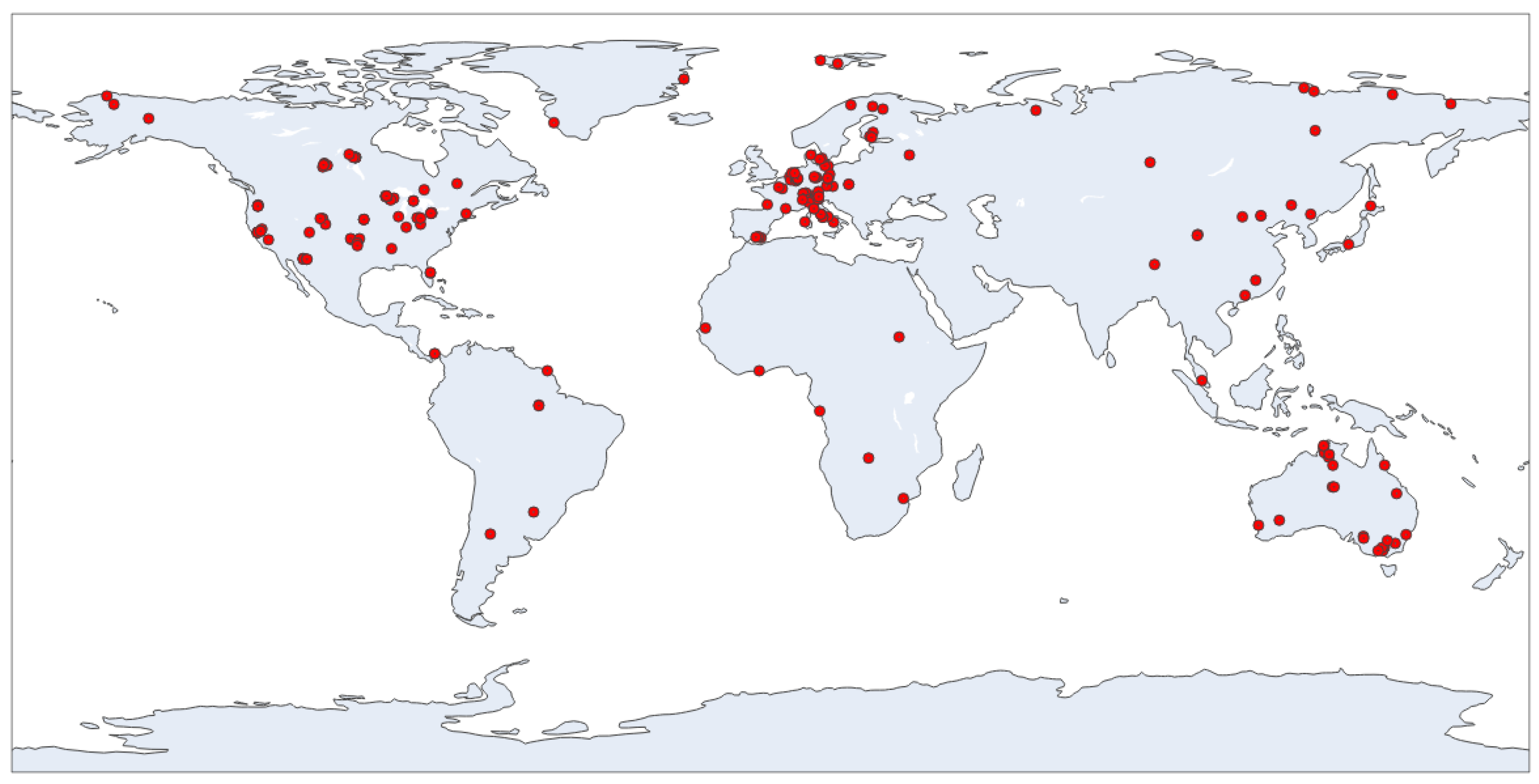
Figure 1. Locations of all Fluxnet sites.
Remotesensing 14 05529 g001
Figure 2. General flowchart of regression model training process.
Remotesensing 14 05529 g002
Figure 3. Left panels are maps of calculated indices for the same date; right panels are maps of daily weight functions for different dates.
Remotesensing 14 05529 g003
Figure 4. Scatterplots of observed NEE vs. predicted NEE based on remote sensing and meteorological features models per each land cover: cropland (CRO); grassland (GRA); evergreen needleleaf forest (ENF); deciduous broadleaf forest (DBF); evergreen broadleaf forest (EBF); mixed forest (MF); wetland (WET); savanna (SAV).
Remotesensing 14 05529 g004
Figure 5. Time series of observed NEE and the predicted NEE based on remote sensing and meteorological features models per each land cover: cropland (CRO); grassland (GRA); evergreen needleleaf forest (ENF); deciduous broadleaf forest (DBF); evergreen broadleaf forest (EBF); mixed forest (MF); wetland (WET); savanna (SAV).
Remotesensing 14 05529 g005aRemotesensing 14 05529 g005b
Figure 6. Comparison of observed and predicted mean NEE for different land covers in this study. Error bars of each land cover are the standard deviation of observed and predicted daily NEE.
Remotesensing 14 05529 g006
Table 1. Example of the aggregated dataset for each feature for each date. Note that the values are scaled by 10,000.
DateBlueNDMISAVI
27 December 2009344.9327.62314.2
28 December 2009346.8345.22335.3
29 December 2009338.3315.52276.5
30 December 2009342.1317.52289.9
31 December 2009355.2355.52392.7
1 January 2010351.3356.42354.5
2 January 2010349.3325.12346.3
3 January 2010351.4361.22373.4
4 January 2010355.4363.22382.4
5 January 2010352.2348.92367.3
Table 2. Example of “target” NEE from eddy covariance stations for each date.
Date NEE , gC / m 2 / Day
27 December 2009−5.77
28 December 2009−7.43
29 December 2009−10.24
30 December 2009−5.49
31 December 2009−7.83
1 January 2010−5.47
2 January 2010−5.24
3 January 2010−3.87
4 January 2010−5.52
5 January 2010−3.45
Table 3. Feature sets for predicting NEE for each IGBP class (detailed description in Appendix B).
Land CoverList of Features
DBF T C G , C u m _ T e m p e r a t u r e _ o v e r _ 5 _ 3 w e e k , b l u e / g r e e n , D e w P o i n t , S o l a r , N I R / S W I R 1 , S W I R 2 / g r e e n , C u m _ p r e c i p i t a t i o n _ 3 d a y s , C u m _ T e m p e r a t u r e _ o v e r _ 5 _ 2 w e e k , C u m _ T e m p e r a t u r e _ o v e r _ 2 _ 1 w e e k , C u m _ T e m p e r a t u r e _ o v e r _ 3 _ 3 w e e k
GRA S W I R 1 / N I R , C u m _ T e m p e r a t u r e _ 1 w e e k , g r e e n / r e d , C u m _ p r e c i p i t a t i o n _ 2 d a y s , M e a n _ S o l a r _ 2 w e e k , D e l t a _ T , r e d / N I R , L S T , N D V I , r e d / g r e e n , g r e e n / N I R , r e d / b l u e , S W I R 2 / S W I R 1 , C u m _ S o l a r _ 4 d a y s , b l u e / N I R , M e a n _ S o l a r _ 4 d a y s
CRO N I R / g r e e n , M e a n _ S o l a r _ 4 w e e k , C u m _ T e m p e r a t u r e _ o v e r _ 5 _ 3 w e e k , N I R / S W I R 2 , D e w P o i n t , b l u e / g r e e n , C u m _ S o l a r _ 2 w e e k , C u m _ T e m p e r a t u r e _ o v e r _ 2 _ 3 w e e k , S W I R 2 / N I R , M e a n _ T e m p e r a t u r e _ 1 w e e k
ENF S o l a r , S W I R 1 / N I R · C u m _ T e m p e r a t u r e _ o v e r _ 5 _ 4 w e e k , C u m _ T e m p e r a t u r e _ o v e r _ 3 _ 3 w e e k , T e m p e r a t u r e A i r , N I R / S W I R 2 · M e a n _ S o l a r _ 2 w e e k , D e l t a _ T , b l u e / S W I R 2 , C u m _ T e m p e r a t u r e _ o v e r _ 4 _ 3 w e e k , N I R / S W I R 2 · S o l a r , N I R · S W I R 1 , C u m _ T e m p e r a t u r e _ 4 d a y s , r e d / S W I R 1
MF T C G · S o l a r , D e l t a _ T , D e w P o i n t , S W I R 2 / b l u e , b l u e / r e d , C u m _ p r e c i p i t a t i o n _ 5 d a y s , T C G · D e w P o i n t , N I R / L S T · S o l a r , N I R · S o l a r
EBF L S T / S W I R 2 · S o l a r , T e m p e r a t u r e A i r , N I R / L S T , C u m _ p r e c i p i t a t i o n _ 2 d a y s , L S T / S W I R 2 · M e a n _ S o l a r _ 1 w e e k , D e l t a _ T , r e d / S W I R 2 · M e a n _ S o l a r _ 2 w e e k
WET N I R · M e a n _ S o l a r _ 3 w e e k , D e l t a _ T , S W I R 1 / N I R , S W I R 1 / g r e e n , C u m _ p r e c i p i t a t i o n _ 3 d a y s , g r e e n · N I R , N D M I , N I R / S W I R 1 , N D V I · M e a n _ S o l a r _ 4 w e e k , T C G · C u m _ T e m p e r a t u r e _ 2 w e e k , T C G · M e a n _ T e m p e r a t u r e _ 4 d a y s , T C G · C u m _ T e m p e r a t u r e _ 4 d a y s , N I R / S W I R 2 , D e w P o i n t , T C G · C u m _ T e m p e r a t u r e _ o v e r _ 4 _ 2 w e e k , T C G · C u m _ T e m p e r a t u r e _ o v e r _ 3 _ 2 w e e k , g r e e n · S W I R 1 , T C G · C u m _ T e m p e r a t u r e _ o v e r _ 2 _ 2 w e e k , S W I R 2 / N I R
SAV N D V I · S o l a r , N I R / S W I R 2 · S o l a r , T e m p e r a t u r e A i r , g r e e n / r e d , r e d / g r e e n , C u m _ T e m p e r a t u r e _ o v e r _ 5 _ 2 w e e k , S W I R 1 / r e d , S W I R 2 / S W I R 1 , E V I · D e w P o i n t , S W I R 1 / g r e e n
Table 4. Cross-validation metrics (and standard deviation of the residuals for each metric) for daily NEE models per land-cover class.
IGBP R 2 RMSE , gC / m 2 / Day RE
CRO0.73 (0.17)2.32 (0.67)0.44 (0.19)
GRA0.61 (0.04)0.70 (0.35)0.60 (0.05)
DBF0.76 (0.05)1.64 (0.16)0.42 (0.04)
ENF0.62 (0.05)1.30 (0.22)0.60 (0.06)
MF0.55 (0.02)1.25 (0.18)0.64 (0.01)
EBF0.42 (0.06)1.28 (0.32)0.73 (0.05)
WET0.53 (0.06)1.55 (0.19)0.64 (0.08)
SAV0.56 (0.03)0.68 (0.14)0.63 (0.02)
Table 5. Cross-validation metrics for monthly NEE values per land-cover class.
IGBP R 2 RMSE , gC / m 2 / Day
CRO0.831.94
GRA0.600.54
DBF0.841.23
ENF0.780.89
MF0.700.75
EBF0.700.80
WET0.661.25
SAV0.690.49
Publisher’s Note: MDPI stays neutral with regard to jurisdictional claims in published maps and institutional affiliations.