Abstract
Mesoscale eddies are typical mesoscale ocean phenomena that exist widely in all oceans and marginal seas around the world, playing important roles in ocean circulation and material transport. They also have important impacts on the safe navigation of ships and underwater acoustic communications. Traditional mesoscale eddy identification methods are subjective and usually depend on parameters that must be pre-defined or adjusted by experts, meaning that their accuracy cannot be guaranteed. With the rise of deep learning, the “you only look once” (YOLO) series target recognition models have been shown to present certain advantages in eddy detection and recognition. Based on sea level anomaly (SLA) data provided over the past 30 years by the Copernicus Marine Environment Monitoring Service (CMEMS), as well as deep transfer learning, we propose a method for oceanic mesoscale eddy detection and identification based on the “you only look once level feature” (YOLOF) model. Using the proposed model, the mesoscale eddies in the South China Sea from 1993 to 2021 were detected and identified. Compared with traditional recognition methods, the proposed model had a better recognition effect (with an accuracy of 91%) and avoided the bias associated with subjectively set thresholds; to a certain extent, the model also improved the detection of and the identification speed for mesoscale eddies. The method proposed in this paper not only promotes the development of deep learning in the field of oceanic mesoscale eddy detection and identification, but also provides an effective technical method for the study of mesoscale eddy detection using sea surface height data.
1. Introduction
Mesoscale eddies are important ocean phenomena that are characterized by closed circulation. They exist in oceans widely and globally and comprise an important part of the ocean structure that cannot be ignored [1]. Compared with ordinary ocean circulation, mesoscale eddies have high rotating speeds (up to several meters per second), strong current velocities, average vertical depths of several kilometers, and maximum vertical depths that can reach the deep seabed. They have a spatial scale of tens to hundreds of kilometers and a time scale of several to hundreds of days [2]. According to their rotation characteristics, mesoscale eddies can be divided into cyclonic and anticyclonic eddies. The typical features of mesoscale eddies are that they can cause strong changes in the heights of sea level, regulate ocean biochemical processes, and significantly impact heat exchange, material transport, chlorophyll concentration, and seawater salinity [3]. In addition, mesoscale eddy energy affects the temperature distribution on the sea surface, resulting in abnormal sea surface temperatures and disrupting the balance of the air–sea coupling system, thus extending their impact to the atmosphere [4]. Mesoscale eddies not only affect the sea surface, but also the sub-surface, as they can reach kilometers below the sea surface and greatly impact the density and speed of sound in sea water. Therefore, it is particularly important to establish a computational model for identifying oceanic mesoscale eddies for the study of ocean currents, marine biology, climate change, and so on.
The detection and identification of oceanic mesoscale eddies provides an important means of monitoring and analyzing the temporal and spatial variation characteristics of mesoscale eddies. Ocean satellite remote-sensing technology has the characteristics of allowing for all-weather, long-distance, non-contact, fast, and efficient observation of ocean phenomena. It can provide rich eddy identification data sources, including data about ocean surface temperatures and altimetry data. Common methods for mesoscale eddy detection and identification mainly include the following: (1) methods based on physical parameters; (2) methods based on the geometric characteristics of the flow field; and (3) methods based on machine learning. Among these methods, physical-parameter-based methods are mesoscale eddy detection methods that are based on physical parameters that can be used to identify the core region and center point of a mesoscale eddy. Isern-Fontanet first proposed the Okubo–Weiss (OW) algorithm in 2003. It is a widely used physical-parameter-based method, but it was not used as a standard method for extracting mesoscale eddies based on sea surface height (SSH) until 2008 [5,6,7].
In the process of detecting and identifying mesoscale eddies, physical-parameter-based methods have great subjectivity and rely excessively on thresholds set according to experts’ experience. Flow field geometry-based methods are a type of global search algorithm based on the custom setting of mesoscale eddies. Represented by the winding angle (WA) algorithm, the eddy region is assumed to be the region obtained after the velocity vector rotates around a central point [8,9]. Although the flow field geometry method can be independent of parameter settings, the calculation process in flow field geometry-based methods is complex, and a significant amount of calculation is required. Neither of these approaches can adapt to the dynamic changes of oceanic eddies that are caused by complex marine environments.
With the development of computational technology and big data, deep learning methods have also been applied to the detection and recognition of oceanic eddies. Using satellite remote-sensing data fusion and reanalysis data, combined with the concept of deep learning, a migration learning network model suitable for identifying oceanic mesoscale eddies can be constructed, where oceanic mesoscale eddies are abstractly learned via the multi-layer structure of the model.
Finally, the automatic detection and recognition of oceanic mesoscale eddies have become research hotspots. In 2017, Du [10] introduced a deep-learning approach for the automatic identification of mesoscale eddies. Based on synthetic aperture radar (SAR) image data, Du proposed a morphological and scale-robust automatic identification model for oceanic mesoscale eddies, which identified highly dynamic oceanic mesoscale eddies. Lguensat et al. [11] applied the U-Net network structure to the feature extraction of oceanic mesoscale eddies in 2018. In the same year, Franz et al. [12] introduced a convolutional neural network for the detection of oceanic mesoscale eddies, and recognized oceanic eddies based on synthetic aperture radar images by combining encoder–decoder and traditional algorithms. In 2019, Xu et al. [13] focused on the detection of small-scale oceanic eddies and adopted the pyramid scene parsing network (PSPNet) algorithm to realize the fusion of multi-scale features of different layers. In 2020, Lu et al. [14] combined the YOLOv3 target detection network in deep learning with the method of extracting mesoscale eddy features in marine physics to identify mesoscale eddies and improve detection speed. In 2021, Xu et al. [15] compared the performance of PSPNet, bilateral segmentation network (BiSeNet), and DeepLabv3+ in oceanic eddy detection and recognition.
In the field of deep learning, the YOLO series target detection models have been widely favored, due to their outstanding detection speed and accuracy. The YOLO algorithm is a typical one-stage method. It is the abbreviation of “you only look once,” which means that the neural network can output the result after only looking at an image once. Among the YOLO models, the YOLOv1 model (released in 2015) and the YOLOv2 model (proposed in 2017) have the characteristic of fast detection speed but are not good at detecting small objects [16,17]. In 2018, Redmon et al. proposed the YOLOv3 model, which improved upon the previous YOLO models [18,19]. The biggest improvement features included the use of the residual model Darknet-53 and feature pyramid network (FPN) architecture to achieve multi-scale detection, thus improving the accuracy of small-object detection and, at the same time, becoming the fastest target-detection model [20].
Based on the original YOLO target detection architecture, YOLOv4 and YOLOv5 have been developed by adopting a series of optimization strategies that are widely used in the field of target detection. In 2021, Chen designed the “you only look once level feature” (YOLOF) model that optimizes the FPN structure. FPN has made great contributions to single-stage target detection and anchor-free target detection, but its network structure is complex. In this line, the YOLOF detection framework does not use complex feature pyramids, but only single-layer feature maps, thereby greatly improving the target detection and recognition performance of the model [21]. In this work, we used state-of-the-art eddy research results as references, in order to solve the problem of mesoscale eddy detection and identification. Our method required a training sample set composed of SLA contour maps, including labelled eddy positions. In this way, the YOLOF model was trained to identify eddies.
This paper is organized as follows: In this Section 1, we detailed the importance and significance of oceanic mesoscale eddies and the related research, listing several of the most widely used and popular methods in oceanic mesoscale eddy detection and providing some basic knowledge regarding YOLO series target detection models. In Section 2, the data sources used in this study and the geographical environment of the South China Sea are introduced. Section 3 focuses on this study’s method for detecting mesoscale eddies and provides a flow chart to facilitate a preliminary understanding of our method. Section 4 includes the results of this study and a corresponding discussion of those results. Finally, Section 5 draws some conclusions, summarizes the deficiencies of the research, and puts forward proposals for future research.
2. Study Area and Data
The study area was the South China Sea (SCS) and its adjacent waters (0–25°N, 100–125°E),as show in Figure 1. The topography of the SCS is complex. The seabed topography is mainly divided into a continental shelf, a continental slope, and a deep-sea basin [22]. Most areas of the SCS are in the tropics and, therefore, they are characterized by a significant tropical marine climate, with mild seasons, abundant rainfall, and monsoons. The SCS is mainly connected to the Northwest Pacific via the Luzon Strait in the northeast. The multi-scale circulation in the basin is significantly controlled by the monsoon and by Pacific water exchange, particularly by the Kuroshio current, which is the strongest western boundary current in the North Pacific. It flows through the east of the Luzon Strait and has far-reaching impacts on the large-scale circulation and mesoscale eddy process in the SCS, in different seasons and in different ways [23,24,25]. Chen et al. [26] observed that the depth of influence of mesoscale eddies in the northern SCS, when mixed with Kuroshio water, can significantly increase, to less than 500 m. In winter, the Kuroshio falls off from the main axis in the form of a flow jacket that can produce strong mesoscale eddies, with a horizontal radius of more than 150 km and a vertical depth of 2000 m [27]. Driven by various dynamic mechanisms, such as wind stress, barotropic/baroclinic instability, and the Kuroshio [28,29,30], mesoscale eddies in the SCS have the characteristics of frequent occurrence, wide coverage, and strong dynamics; furthermore, multi-eddy phenomena, such as eddy pairs and eddy groups, are common [31,32]. Therefore, the clear driving mechanism and complex internal eddy structures make the SCS a natural test site for oceanic mesoscale eddy research [33,34].
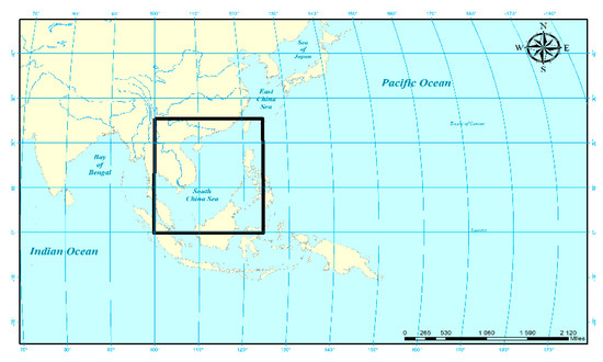
Figure 1.
Study area (0°–25°N, 100°–125°E).
The sea surface height data used in this study are products of the SSALTO/DUACS altimeter, with spatial resolution of 0.25° × 0.25°, temporal resolution of 1 d, and the data format network common cata form (NetCDF). Released by the French Archiving, Validation and Interpretation of Satellite Oceanographic data portal (AVISO+), it is a multi-task fusion altimeter data product. At present, the dataset is processed and distributed by the Copernicus Marine Environment Monitoring Service (CMEMS) (https://resources.marine.copernicus.eu/product-detail, accessed on 24 October 2022). The altimeter satellite grid sea level anomaly (SLA) is calculated based on the average value during the 20 years before 2012. The SLA is estimated by optimal interpolation, combining measurements from different available altimeter missions. The product is processed by the DUACS multi-mission altimeter data processing system, which processes data from various altimeter missions, including Jason-3, Sentinel-3A, HY-2A, Saral/AltiKa, Cryosat-2, Jason-2, Jason-1, T/P, EN-VISAT, GFO, and ERS1/2. Finally, the processing system obtains and synchronizes altimeter and auxiliary data [35].
Each task uses the same model and correction method for homogenization. The multi-task cross calibration process eliminates any residual orbit error or long wavelength error and large-scale deviations between various data streams. All altimeter fields are interpolated at the intersection position and date [36]. After repeated trajectory analysis, the average profile or average sea surface unique to each mission (when the orbit is not repeated) is subtracted to calculate the SLA. Geostrophic currents are derived from the SLA (in terms of geostrophic velocity, ugos, and vgos). Multi-satellite data fusion not only effectively reduces the mapping error of SLA data, but also effectively improves the temporal and spatial resolution. In this study, SLA data from January 1993 to December 2021 were used for the detection of eddies. The data from 1 January 1993, to 31 December 2020, were used to form the training and verification sets, in order to fit the model and adjust the model parameters, respectively, while the remaining (2021) data were used as the test set, in order to evaluate the generalization ability of the final model. In this data, we removed the shelf areas with depths of less than 200 m.
3. Methods
The deep learning algorithm proposed in this study was based on the method of deep transfer learning combined with the YOLOF model for the detection and identification of oceanic mesoscale eddies. The flow chart of the algorithm framework is shown in Figure 2, which includes four stages: (1) sample pre-processing, in which the remote sensing satellite altimeter data are pre-processed and the SLA sample dataset is formed; (2) pretraining, in which the labeled training set (A1) is input into the YOLOF detection model for training and verification; (3) transfer learning, where the initial weight parameters obtained from the pretraining are transferred to the training set (A2); and (4) model detection and recognition, in which the test set is used in the trained YOLOF model for the detection and recognition of oceanic mesoscale eddies. The specific details of the stages are detailed in the following figure.
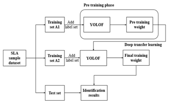
Figure 2.
Technical roadmap of identification scheme.
In the sample pre-processing stage, we pre-processed the remote sensing satellite altimeter data to form the SLA sample dataset. The sample set included a picture set and a label set. The information in the picture set included SLA and geostrophic current velocity, which were used as input to the YOLOF detection model. The data were visualized via contour lines, vector lines, and color maps. The interval between contours was measured in centimeters. The land part was masked by not-a-number (NaN) values, helping to avoid outliers and detection interference. The label set contained eddy position and category information in each picture. The pre-processed sample set was divided into a training set, a validation set, and a test set.
For all satellite products, the calculation formula for SLA was as follows:
where SSH is the sea surface height and MP is mean profile, representing the most accurate mean sea surface (MSS). The most precise MSS is available on long-term repeat tracks [37].
SLA = SSH − MP
The speed of geostrophic velocity was calculated as follows:
where u and v represent the zonal and meridional components of the geostrophic current velocity, g denotes gravitational acceleration, f is the Coriolis parameter, and ξ is the SLA.
The label set was constructed using the eddy identification method and code py-eddy-detection released by the CMEMS for reference, in order to identify the mesoscale eddies from SLA data. This established the corresponding regression fitting formula between the longitude and latitude information of the eddy boundary and the coordinates of the label frame, and automatically generated high-precision label frames.
The traditional methods of oceanic mesoscale eddy annotation are generally carried out via visual annotation by experts in advance. However, since experts’ visual annotation can only label oceanic mesoscale eddy for a small number of samples, and the deep learning model requires a great deal of data to avoid overfitting in the model, data enhancement, such as flipping, clipping, rotating, and scaling [38], is required for this part of the visual image to increase the size and quality of the training set [39,40]. Due to the difference between the generated image and the real image, noise and other shortcomings are inevitable, and the data enhancement implementation is manually designed. Even though there are many data enhancement strategies that can optimize a generated image, there is still a gap between the credibility of the generated image and that of the real image.
In this paper, the real images were automatically annotated to avoid the limitations of data enhancement methods. This method was based on the geostrophic equilibrium state. The SLA isoline can approximately replace the streamline isoline. While improving the calculation efficiency, it retains the change of observation signal to the greatest extent and reduces the error caused when artificially determining the threshold [41]. The basic principle was to identify eddies by retrieving closed SLA contours. Each closed contour as screened with respect to criteria related to the shape and internal characteristics of eddies. When the closed contour passed these criteria, it was identified as belonging to an eddy; the outermost contour provided the actual shape of the detected eddy. The eddy profile screening criteria were as follows:
- (1)
- In the shape inspection, the shape error was ≤ 55%, where the shape error E was calculated using the following formula:where is the area of the closed contour, is the area of the contour-fitting circle, and is the overlapping area between and ;
- (2)
- A certain number of pixels i were included, satisfying 8 ≤ i ≤ 1000;
- (3)
- Only pixels with SLA values above (below) the current SLA interval value for anticyclonic (cyclonic) eddies were contained;
- (4)
- For cyclonic eddies (anticyclonic eddies), there was at most one SLA minimum (maximum);
- (5)
- Considering the error of the data, the amplitude A of the eddy had to meet 1 ≤ A ≤ 150 cm, where A is defined as the absolute value of the difference between the SLA value of the outermost contour and the extreme value in the contour.
Although it was confirmed that a calculation step of 1 cm is sufficient to solve for an eddy with compact internal space, we found that a smaller step was preferable, as this could better approximate the shape of eddy fluid [42,43]. However, as the altimeter measurement error was generally between 2 cm to 3 cm, the amplitude of the identified mesoscale eddy should not be less than 2 cm to 3 cm. Combined with the actual situation of the SCS, in order to accurately detect a small-scale eddy, the eddy amplitude in this study should not have been less than 2 cm.
In the pretraining stage, after adding label information to the training and verification sets, we input the labeled training set A1 into the YOLOF detection model for training and verification. The reason for choosing the YOLOF model for the detection and identification of oceanic mesoscale eddies was that YOLOF is optimized, in terms of the FPN. The YOLOF model does not need to use a complex feature pyramid, and only requires a single-layer feature map to learn the characteristics of oceanic eddies when obtaining the initial weights in model training. Experiments on coco datasets have proved the effectiveness of YOLOF. It obtained the same results as the characteristic pyramid version, but with 2.5 times faster speed. In addition, without the transformer layer, YOLOF is comparable to DETR, which also uses a single-layer feature map.
The YOLOF detection framework is a new target-detection approach, using only 32× down-sampled C5 feature maps. In order to make up for the performance gap between single-input single-output (SiSo) and multiple-input multiple-output (MiMo) encoders, the structure of the encoder is properly designed to extract the multi-scale context features of different scale targets, thus making up for the deficiencies regarding multi-scale features. Then, the balanced matching mechanism is used to solve the problem of positive sample imbalance caused by sparse anchors in the single feature graph. The YOLOF detection framework consists of three main parts: backbone, encoder, and decoder. The network architecture is depicted in Figure 3.
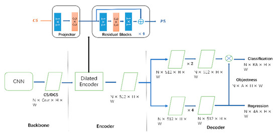
Figure 3.
Network structure chart.
The backbone adopts the classic RESNET and ResNeXt. The selected characteristic diagram is C5, the number of channels is 2048, and the down-sampling rate is 32 [44].
The encoder was used to accept input from the backbone and assign a representation for detection. It comprises two components: namely, projector and residual. The projector first applied a 1 × 1 convolution to reduce the channel dimension, and then added a 3 × 3 convolution layer to refine the context semantic information, thus obtaining a characteristic graph with 512 channels, consistent with the FPN. Residual blocks included residual modules with different expansion rates, which generated output features with multiple acceptance domains covering the scales of all objects in order to provide a full-scale receptive field. The residual module consisted of three consecutive convolutions: the first was a 1 × 1 convolution, which reduced the channel dimension, following which a 3 × 3 convolution was used to expand the receptive field. Finally, 1 × 1 convolution restored the dimensions of the channel. This residual block was repeated four times [45].
The decoder was used to perform classification and regression tasks, thus generating the final prediction box. Like RetinaNet, the decoder contained two parallel task-specific heads: the classification head was used for the target classification task, while the regression head was used for the border regression task. The decoder was designed according to the FFN in DETR, such that the number of two-headed convolution layers differed. In the regression branch, there were four convolution layers plus a BN layer and an ReLU layer; meanwhile, in the classification branch, there were only two convolution layers. Second, according to Autoassign, an implicit Objectness (without direct supervision) was added to each anchor of the regression branch. The final classification confidence was obtained by multiplying the output of the classification branch and the Objectness score [46].
In the transfer learning stage, the YOLOF model was also used to train and verify the training set A2, where the initial weights from the previous step were used for the transfer learning of the model. The final training weights were generated by continuing to learn the characteristics of oceanic eddies. Deep transfer learning is a kind of technique used to study how to use DNNs to transfer knowledge from other fields [47]. According to different types of migration methods, it can be divided into four categories: (1) instance-based deep transfer learning, which refers to the selection of some instances in the training set from the source domain to the target domain [48]; (2) mapping-based deep transfer learning, which refers to mapping some instances from the source domain and target domain to a new data space [49]; (3) network-based deep transfer learning, which refers to re-using part of the network and connection parameters in the source domain, migrating them to a part of the deep neural network used in the target domain [50]; and (4) network-based deep transfer learning, which refers to the introduction of antagonistic technologies (e.g., GAN) to find transferable formulas suitable for the source and target domains [51].
In the model detection and identification stage, the test set was used to validate the final model, and the mean average precision (mAP) was used as an evaluation index. First, the accuracy of the border could be expressed by the intersection over union (IoU). In the target detection, the detection network sorted the detection results according to the confidence scores and assigned them to the ground truth objects. We had a “match” when they shared the same label and an IoU of ≥0.5 (i.e., an IoU greater than 50%). Such a match was considered a true positive if the ground truth object had not been already used, in order to avoid multiple detections of the same object [52]. The threshold was generally set to 0.5; that is, if IoU ≥ 0.5, it was considered that the detection was correct. The TP, FP, and FN rates could be calculated using the IoU. Then, taking the recall rate as the abscissa and the accuracy rate as the ordinate, the P–R curve could be obtained. Ideally, the accuracy rate and recall rate would be infinitely close to 1 at the same time. Therefore, we hoped that the area covered under the P–R curve was infinitely close to 1. We called the area obtained below the P–R the accurate mean rate of detecting mesoscale eddies, or the average precision (AP). The AP of multiple categories was averaged, providing the mean AP (mAP). The IOU, precision, recall, and AP were defined as follows:
where Area of Overlap refers to the intersection of two prediction frames, Area of Union is the union of two prediction frames, TP refers to the number of eddies recognized as eddies by the model, FP represents the number of other objects recognized as eddies, and FN refers to the number of eddies recognized as other objects.
4. Results and Discussion
4.1. Detection Results of YOLOF Model
The dataset used in this study contained 10,592 images, divided into training set A1 (1096 images), training set A2 (9131 images), and the test set (365 images). Training set A1 was used for training and verifying the detection model in the pretraining stage, while training set A2 was used to train and verify the model. The remaining images were used as a test set to validate the final model.
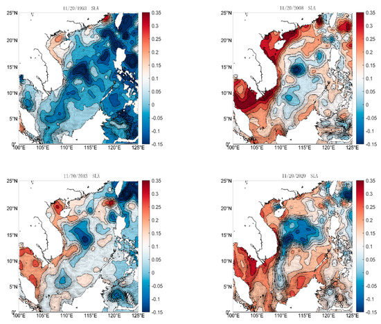
Figure 4.
Sample set after pretreatment.
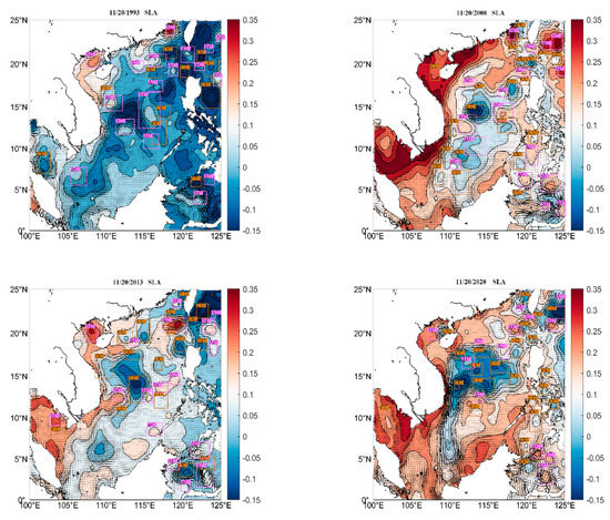
Figure 5.
Label set visualization (CC represents cyclonic and AC represents anticyclonic).
We first input the training set A1 and the corresponding label file into the YOLOF model for pretraining and verification. The parameters in the base configuration (base config) file of the YOLOF model in the pretraining stage included the following: IMS per batch, which refers to the number of samples sent by the network to the model during each training phase; base LR (the base learning rate), which is the initial learning rate and refers to how much the network weights are updated in the optimization algorithm; warm-up, which refers to the preheating factor that forces the learning rate to slowly increase up to the initial learning rate; and warm-up_iters and the max iter, which refer to the number of warm-up iterations and the maximum number of iterations, respectively. The training results were saved once every 1500 iterations. The parameters were adjusted to obtain the best performance of the model. The details of the parameters are provided in Table 1.

Table 1.
Base configuration (base config) file parameters of the pretraining model.
The model mAP in the pretraining stage was approximately 83%. The outputs of the training and verification results by the YOLOF model after pretraining are shown in Figure 6.
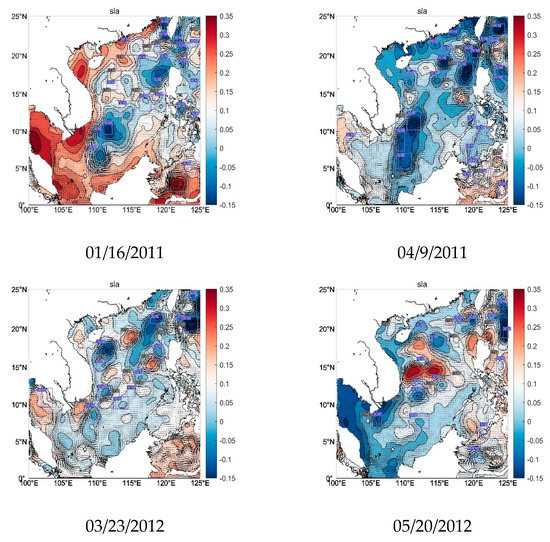
Figure 6.
Verification results in pretraining stage(CC represents cyclonic and AC represents anticyclonic).
Then we, transferred the model weight parameter file obtained in the pretraining stage for the training and verification of training set A2 in the YOLOF detection model, in order to obtain the final model weight parameters. The parameters in the Base-config file of the detection model were modified, according to the sample size. The parameter data are provided in Table 2.
Table 2.
Base config file parameters of the pretraining model.
The mAP of training set A2 trained and verified on the YOLOF model was approximately 90%. The final generated model weight parameter file was used to test the model. On the test set, the mAP of the trained YOLOF detection model was 91.3%. The evaluation index results of different stages are shown in Table 3, and the YOLOF model used in this paper was compared with a traditional eddy detection model; the results are shown in Table 4.
Table 3.
Evaluation index results of different stages.
Table 4.
Detection accuracy of different eddy detection models.
The oceanic mesoscale eddy identification results of the YOLOF detection model on the test set are depicted in Figure 7.
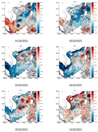
Figure 7.
Test set results (CC represents cyclonic and AC represents anticyclonic).
4.2. Analysis of Mesoscale Eddy Parameters
Considering the characteristic properties of oceanic mesoscale eddies, we conducted the following analysis:
- (1)
- The radius (R) of the eddy was analyzed. The shape of a mesoscale eddy was typically irregular. In this paper, the average geographical distance between the eddy center and the outermost of the four fields was considered as the radius (R) of the mesoscale eddy, using the following formula:
- (2)
- The amplitude (A) of the eddy was also analyzed; it refers to the absolute value of the height difference between the extreme value of the SLA in the eddy center and the SLA around the effective contour defining the eddy edge, as determined by the following formula:
- (3)
- We analyzed the eddy kinetic energy (EKE), as generally high kinetic energy can be observed in ocean areas with strong mesoscale eddy activity. The calculation formula under the geostrophic assumption is as follows (u and v were introduced in Section 3):
For the analysis of the R, A, and EKE values of mesoscale eddies, only 20 November 2021, was taken as an example. Table 5 provides specific information of the R, A, and EKE values of 14 cyclonic eddies and 11 anticyclonic eddies detected and identified on 20 November 2021. It can be seen from the information in the table that the amplitudes of the cyclonic and anticyclonic eddies were mostly concentrated in the range of 2.0 cm to 6.0 cm. The average amplitude of mesoscale eddies in the study area was 4.7 cm, the average amplitude of cyclonic eddies was 4.1 cm, the average amplitude of anticyclonic eddies was 5.5 cm, the maximum amplitude of cyclonic eddies was 10.5 cm, and the maximum amplitude of anticyclonic eddies was 14.2 cm. The eddy radius values also presented similar characteristics. With a radial difference of 15 km, a different distribution will be presented between eddies. The average radius of the detected mesoscale eddies was 89.38 km, where the average radius of cyclonic eddies was 86.23 km and the average radius of anticyclonic eddies was 93.39 km. The radius was mostly concentrated in the range of 57 km to 136 km, but the ranges of the radius and amplitude for anticyclonic eddies were wider. From the attribute analysis diagram of cyclonic and anticyclonic eddies (Figure 8 and Figure 9), it can be seen that the eddies with small amplitudes generally had small eddy kinetic energy, while the eddies with large amplitudes carried high energy, thus affecting the propagation of oceanic kinetic energy. Figure 10 shows the EKE diagram of oceanic mesoscale eddies.
Table 5.
Eddy characteristic information.
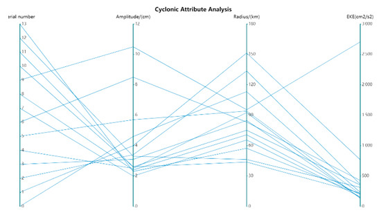
Figure 8.
Cyclonic attribute analysis.
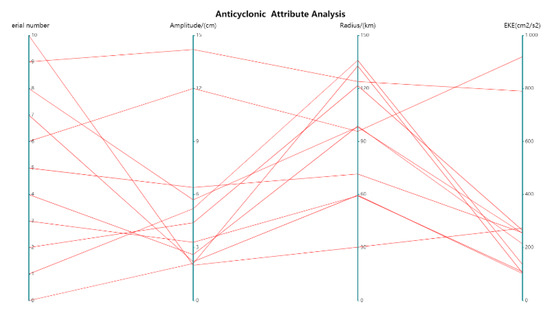
Figure 9.
Anticyclonic attribute analysis.
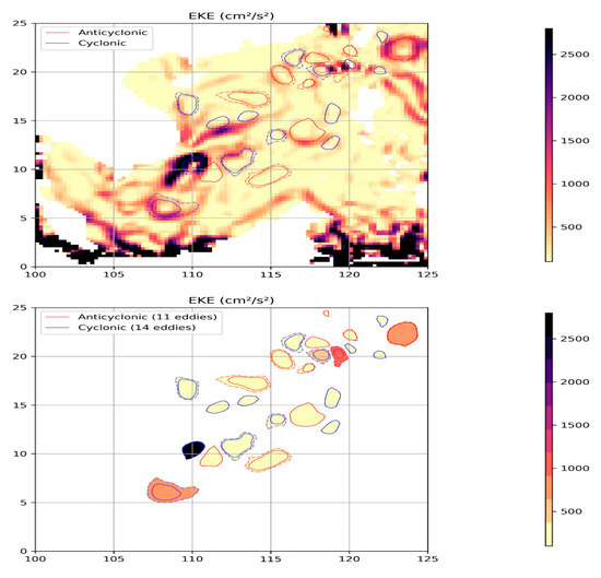
Figure 10.
EKE map of oceanic mesoscale eddies.
4.3. Temporal Analysis of Mesoscale Eddies
To determine the statistics of the number of oceanic mesoscale eddies and to carry out time-series analysis of the eddies, only the oceanic mesoscale eddies detected and identified in the study area of the test set in 2021 were analyzed. Figure 11 shows the variation in the number of mesoscale eddies observed each day. Cyclonic and anticyclonic eddies presented fluctuating changes. Without considering the eddy life cycle, a total of 11,454 mesoscale eddies were detected, including 5329 anticyclonic eddies and 6125 cyclonic eddies; that is, the daily average number of anticyclonic eddies was approximately 15 and the daily average number of cyclonic eddies was approximately 17. The eddies were mainly distributed in the northeast and southwest sea areas with a water depth of more than 200 m. Among them, the western sea area of the Luzon Strait was the most significant mesoscale eddy phenomenon area; it was mainly concentrated to the southwest of Taiwan Island. In addition, the western boundary of the basin and the sea area to the west of Luzon Island also experienced frequent eddies and, in the western boundary sea area of the basin (i.e., the sea off the east of Vietnam), eddies were more active, mainly south and north of the basin. Figure 12 shows the monthly variations of the mesoscale eddies. The cyclonic eddies occurred mostly in April and least in December, while the anticyclonic eddies occurred mostly in July and least in January. In the study area of this paper, the mesoscale eddies were widely distributed throughout the four seasons, but the generation of mesoscale eddies presented obvious seasonal changes: spring and summer were high-incidence seasons, while the number of mesoscale eddies in autumn and winter decreased significantly.
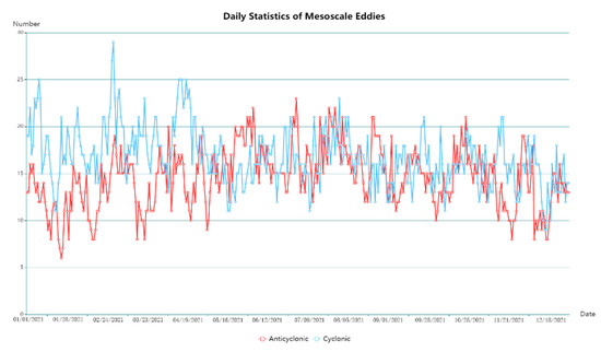
Figure 11.
Daily statistics of mesoscale eddies.
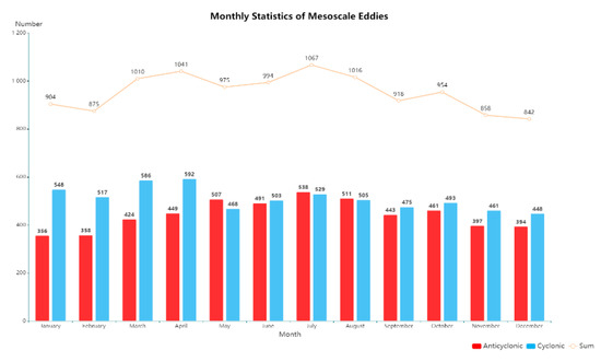
Figure 12.
Monthly statistics of mesoscale eddies.
4.4. Discussion
Cyclonic eddies were most active in winter and spring, with the number being generally higher during those seasons than the number of anticyclonic eddies in the same period. The end of winter and the beginning of spring are usually the periods with the strongest wind forces, annually. In this context, the strong cyclonic wind stress curl enters the upper sea water, and the wind-driven Kuroshio current frequently invades the South China Sea. Under the influence of the land slope topography and the local circulation on the seabed, a large-scale cyclone circulation is formed in the upper layer of the South China Sea, which is more conducive to the generation and survival of cyclonic eddies. Then, the wind gradually weakens and the monsoon changes, such that the ocean’s current flow direction becomes relatively disordered. Until the southwest monsoon begins to prevail in summer, more cyclonic eddies disappear during this process, resulting in a sharp decrease in the number in summer. Furthermore, the intrusion of the Kuroshio in summer is greatly weakened. Yuan et al. [30] found that the anticyclonic eddy generated near the Luzon Strait in summer was different from the water properties of the Kuroshio. Combined with the seasonal variations in the wind stress curl, it is considered that the anticyclonic eddies in this season are formed by the near-shore water driven by the southwest monsoon. Autumn also comprises the transition period of monsoon transformation. Compared with summer, the Kuroshio invasion increases significantly, the number of cyclonic eddies increases, and the number of anticyclonic eddies generally presents a downward trend. The difference, here, is that the number of cyclonic eddies did not rise in autumn in the study area. The reason for this phenomenon may be that the YOLOF model did not sufficiently learn the characteristics of cyclonic eddies, resulting in no significant increase in the number of cyclonic eddies detected. It should be considered that the YOLOF model has not previously been applied in the field of eddy recognition; there are inherent differences in SLA processing in the production stage of the sample set, and it remains to be determined whether the eddy identification standard should be stricter. These factors all may affect the accuracy of the YOLOF detection and identification model.
5. Conclusions
This study combined the YOLOF target-detection and recognition network based on deep learning with the method of extracting mesoscale eddy features in marine physics and adjusted the relevant parameters of the YOLOF target-detection model for training. Using the SSAL-TO/DUACS altimeter products from 1993 to 2020, the SLA sample dataset for deep learning was constructed for the research area (spanning 0–25°N, 100–125°E). For the label set of the sample dataset, the SLA closed-contour method was used to determine the corresponding rules, establish the corresponding regression fitting relationship between the longitude and latitude of the eddy boundary and the coordinates of the label frame, and automatically generate high-precision label frames. In the pretraining phase, the model can preliminarily understand the significant characteristics of oceanic mesoscale eddies. In the transfer-learning phase, we used another training set (A2) to train and verify the detection model, while its initial weights were transferred from the YOLOF model, trained with training set A1. This was a typical network-based deep transfer-learning method, which can improve the stability and accuracy of the model. After model pretraining and transfer training, and after adjusting relevant parameters of the YOLOF target-detection model, the final trained and verified model was used to detect mesoscale eddies in the study area in 2021, in which ideal detection results were obtained: i.e., the detection mAP reached 91.3%. The experimental results indicated that, compared with the traditional methods of identifying oceanic mesoscale eddies, the method proposed in this paper had good detection effect, avoided the influence of threshold selection, and greatly improved the speed of eddy detection.
However, at present, a key limitation of the current model is that we only used sea level height anomaly data with a resolution of 0.25° × 0.25° for training. In future research work, we hope to train a model using SLA data with higher resolution or sea surface temperature anomaly data, in order to improve the average accuracy of the obtained detection and recognition results. In addition, the number of training rounds used were not sufficient, so the model may not have learned enough about the characteristics of oceanic mesoscale eddies, leading to some errors. Moreover, the generalization ability of the oceanic mesoscale eddy detection and recognition model based on YOLOF, as proposed in this paper, was not verified. Finally, the detection of the three-dimensional mechanism of oceanic mesoscale eddies by means of satellite remote sensing is a key research topic that remains to be explored in the future.
Author Contributions
Conceptualization, L.C. and D.Z.; methodology, L.C. and X.Z.; validation, L.C. and Q.G.; writing—original draft preparation, L.C., D.Z. and X.Z.; writing—review and editing, D.Z. and X.Z. All authors have read and agreed to the published version of the manuscript.
Funding
This research was funded by the National Natural Science Foundation of China (No. 42001274).
Data Availability Statement
The data underlying the results presented in this paper can be ob-tained from the authors upon reasonable request.
Acknowledgments
The authors would like to acknowledge the anonymous reviewers for their valuable comments.
Conflicts of Interest
The authors declare no conflict of interest.
References
- Ikeda, M.; Mysak, L.A.; Emery, W.J. Observation and Modeling of Satellite-Sensed Meanders and Eddies off Vancouver Island. J. Phys. Oceanogr. 1984, 14, 3–21. [Google Scholar] [CrossRef]
- Zhao, Y. Analysis of Sound Propagation in Mesoscale Eddy Environment; Ocean University of China: Shandong, China, 2015. [Google Scholar]
- Wang, Q.; Li, W.; Ma, J.; Han, G.; Zhang, X. Study on the meso-scale process of the Kuroshio front to the east of Taiwan. Mar. Sci. Bull. 2011, 13, 518–528. [Google Scholar]
- Ma, X.; Jing, Z.; Chang, P.; Liu, X.; Montuoro, R.; Small, R.J.; Bryan, F.O.; Greatbatch, R.J.; Brandt, P.; Wu, D.; et al. Western boundary currents regulated by interaction between ocean eddies and the atmosphere. Nature 2016, 535, 533–537. [Google Scholar] [CrossRef] [PubMed]
- Haller, G.; Hadjighasem, A.; Farazmand, M.; Huhn, F. Defining Coherent Eddies Objectively from the Vorticity. J. Fluid Mech. 2016, 795, 136–173. [Google Scholar] [CrossRef]
- Henson, S.; Thomas, A. A census of oceanic anticyclonic eddies in the Gulf of Alaska. Deep Sea Res. Part I Oceanogr. Res. Pap. 2008, 55, 163–176. [Google Scholar] [CrossRef]
- Isern-Fontanet, J.; Garcí a-Ladona, E. Identification of Marine Eddies from Altimetric Maps. J. Atmos. Ocean. Technol. 2003, 20, 772–778. [Google Scholar] [CrossRef]
- Isern-Fontanet, J.; Garcí a-Ladona, E. Eddies of the Mediterranean Sea: An Altimetric Perspective. J. Phys. Oceanogr. 2006, 36, 87–C103. [Google Scholar] [CrossRef]
- Sadarjoen, I.A.; Post, F.H. Detection, quantification, and tracking of eddies using streamline geometry. Comput. Graph. 2000, 24, 333–341. [Google Scholar] [CrossRef]
- Du, Y. Automatic Identification of Mesoscale Eddies Based on Ocean Remote Sensing Images and Its Relationship with Fishing Ground Dynamics; Shanghai Ocean University: Shanghai, China, 2017. [Google Scholar]
- Lguensat, R.; Sun, M.; Fablet, R.; Tandeo, P.; Mason, E.; Chen, G. EddyNet: A Deep Neural Network for Pixel-Wise Classification of Oceanic Eddies. In Proceedings of the 2018 IEEE International Geoscience and Remote Sensing Symposium, Valencia, Spain, 22–27 July 2018. [Google Scholar]
- Franz, K.; Roscher, R.; Milioto, A.; Wenzel, S.; Kusche, J. Ocean Eddy Identification and Tracking Using Neural Networks. In Proceedings of the 2018 IEEE International Geoscience and Remote Sensing Symposium, Valencia, Spain, 22–27 July 2018. [Google Scholar]
- Xu, G.; Cheng, C.; Yang, W.; Xie, W.; Kong, L.; Hang, R.; Ma, F.; Dong, C.; Yang, J. Oceanic Eddy Identification Using an AI Scheme. Remote Sens. 2019, 11, 1349. [Google Scholar] [CrossRef]
- Lu, X.; Gui, S.; Li, G. Ocean mesoscale eddy recognition and visualization based on deep learning. Comput. Syst. Appl. 2020, 29, 65–75. [Google Scholar]
- Xu, G.; Xie, W.; Dong, C.; Gao, X. Application of Three Deep Learning Schemes into Oceanic Eddy Detection. Front. Mar. Sci. 2021, 8, 715. [Google Scholar] [CrossRef]
- Redmon, J.; Divvala, S.; Girshick, R.; Farhadi, A. You only look once: Unified, real-time object detection. In Proceedings of the 2016 IEEE Conference on Computer Vision and Pattern Recognition, Las Vegas, NV, USA, 26–27 June 2016; pp. 779–788. [Google Scholar]
- Redmon, J.; Farhadi, A. Yolo9000: Better, faster, stronger. In Proceedings of the 2017 IEEE Conference on Computer Vision and Pattern Recognition, Honolulu, HI, USA, 21–26 July 2017; pp. 7263–7271. [Google Scholar]
- Liu, Z.; Gu, X.; Yang, H.; Wang, L.; Chen, Y.; Wang, D. Novel YOLOv3 model with structure and hyperparameter optimization for detection of pavement concealed cracks in GPR images. In IEEE Transactions on Intelligent Transportation Systems; IEEE: Piscataway Township, NJ, USA, 2022; pp. 1–11. [Google Scholar]
- Wang, D.; Liu, Z.; Gu, X.; Wu, W.; Chen, Y.; Wang, L. Automatic Detection of Pothole Distress in Asphalt Pavement Using Improved Convolutional Neural Networks. Remote Sens. 2022, 14, 3892. [Google Scholar] [CrossRef]
- Tan, M.; Pang, R.; Le, Q.V. Efficient det: Scalable and efficient object detection. In Proceedings of the 2020 IEEE/CVF Conference on Computer Vision and Pattern Recognition, Seattle, WA, USA, 13–19 June 2020; pp. 10781–10790. [Google Scholar]
- Chen, Q.; Wang, Y.; Yang, T.; Zhang, X.; Cheng, J.; Sun, J. You Only Look One-level Feature. In Proceedings of the 2021 IEEE/CVF Conference on Computer Vision and Pattern Recognition, Nashville, TN, USA, 20–25 June 2021; pp. 13034–13043. [Google Scholar]
- Wu, M. Identification, Tracking and Characteristic Analysis of Mesoscale Eddies in the South China Sea; Guilin University of Technology: Guangxi, China, 2021. [Google Scholar]
- Yuan, D.; Han, W.; Hu, D. Surface Kuroshio path in the Luzon Strait area derived from satellite remote sensing data. J. Geophys. Res. Ocean. 2006, 111, C11007. [Google Scholar] [CrossRef]
- Metzger, E.J.; Hurlburt, H.E. The nondeterministic nature of Kuroshio penetration and eddy shedding in the South China Sea. J. Phys. Oceanogr. 2001, 31, 1712–1732. [Google Scholar] [CrossRef]
- Caruso, M.J.; Gawarkiewicz, G.G.; Beardsley, R.C. Interannual variability of the Kuroshio intrusion in the South China Sea. J. Oceanogr. 2006, 62, 559–575. [Google Scholar] [CrossRef]
- Chen, G.; Hou, Y.; Chu, X.; Qi, P. Vertical structure and evolution of the Luzon warn eddy. Chin. J. Oceanol. Limnol. 2010, 28, 955–961. [Google Scholar] [CrossRef]
- Li, L.; Nowlin, W.D., Jr.; Su, J. Anticyclonic Rings from the Kuroshio in the South China Sea. Deep Sea Res. Part I Oceanogr. Res. Pap. 1998, 45, 1469–1482. [Google Scholar] [CrossRef]
- Xue, H.; Chai, F.; Pettigrew, N.; Xu, D.; Shi, M.; Xu, J. Kuroshio Intrusion and the Circulation in the South China Sea. J. Geophys. Res. Oceans 2004, 109. [Google Scholar] [CrossRef]
- Chen, R.; Flied, G.R.; Wunsch, C. A description of local and nonlocal eddy-mean flow interaction in a global eddy-permit-ting state estimate. J. Phys. Oceanography 2014, 44, 2336–2352. [Google Scholar] [CrossRef]
- Yuan, D.; Han, W.; Hu, D. Anti-cyclonic eddies northwest of Luzon in summer-fall observed by satellite altimeters. Geophys. Res. Lett. 2007, 34, L13610. [Google Scholar] [CrossRef]
- Nan, F.; He, Z.; Zhou, H.; Wang, D. Three long-lived anticyclonic eddies in the northern South China Sea. Geophys. Res. Ocean. 2011, 116. [Google Scholar] [CrossRef]
- Zheng, Q.; Hu, J.; Zhu, B.; Feng, Y.; Jo, Y.-H.; Sun, Z.; Zhu, J.; Lin, H.; Li, J.; Xu, Y. Standing wave modes observed in the South China Sea deep basin. J. Geophys. Res. Ocean. 2014, 119, 4185–4199. [Google Scholar] [CrossRef]
- Liu, Q.; Kaneko, A.; Su, J. Recent progress in studies of the South China Sea circulation. J. Oceanogr. 2008, 64, 753–762. [Google Scholar] [CrossRef]
- Tian, J.; Qu, T. Advances in research on the deep South China Sea circulation. Chin. Sci. Bull. 2012, 57, 1827–1832. [Google Scholar] [CrossRef]
- Faghmous, J.H.; Frenger, I.; Yao, Y.; Warmka, R.; Lindell, A.; Kumar, V. A daily global mesoscale ocean eddy dataset from satellite altimetry. Sci. Data 2015, 2, 150028. [Google Scholar] [CrossRef] [PubMed]
- Amores, A.; Jordà, G.; Arsouze, T.; Le Sommer, J. Up to what extent can we characterize ocean eddies using present-day gridded altimetric products. J. Geophysics. Res. Ocean 2018, 123, 7220–7236. [Google Scholar] [CrossRef]
- Pujol, M.I.; Faugère, Y.; Taburet, G.; Dupuy, S.; Pelloquin, C.; Ablain, M.; Picot, N. DUACS DT2014: The new multi-mission altimeter dataset reprocessed over 20 years. Ocean Sci. Discuss. 2016, 12, 1067–1090. [Google Scholar] [CrossRef]
- Liu, Z.; Gu, X.; Wu, W.; Zou, X.; Dong, Q.; Wang, L. GPR-based detection of internal cracks in asphalt pavement: A combination method of DeepAugment data and object detection. Measurement 2022, 197, 111281. [Google Scholar] [CrossRef]
- CAngermann, C.; Haltmeier, M. Deep structure learning using feature extraction in trained projection space. Comput. Electr. Eng. 2021, 92, 107097. [Google Scholar] [CrossRef]
- Nadimi, E.S.; Buijs, M.M.; Herp, J.; Kroijer, R.; Kobaek-Larsen, M.; Nielsen, E.; Pedersen, C.D.; Blanes-Vidal, V.; Baatrup, G. Application of deep learning for autonomous detection and localization of colorectal polyps in wireless colon capsule endoscopy. Comput. Electr. Eng. 2020, 81, 106531. [Google Scholar] [CrossRef]
- Souza, J.M.A.C.; De Boyer Montegut, C.; Le, T.P.Y. Comparison between three implementations of automatic identification algorithms for the quantification and characterization of mesoscale eddies in the South Atlantic Ocean. Ocean. Sci. 2011, 7, 317–334. [Google Scholar] [CrossRef]
- Faghmous, J.H.; Le, M.; Uluyol, M.; Kumar, V.; Chatterjee, S. A parameter-free spatio-temporal pattern mining model to catalog global ocean dynamics. In Proceedings of the 2013 IEEE 13th International Conference on Data Mining, Dallas, TX, USA, 7–10 December 2013. [Google Scholar]
- Yi, J.; Du, Y.; He, Z.; Zhou, C. Enhancing the accuracy of automatic eddy detection and the capability of recognizing the multi-core structures from maps of sea level anomaly. Ocean. Sci. 2014, 10, 39–48. [Google Scholar] [CrossRef]
- Xie, S.; Girshick, R.; Dollár, P.; Tu, Z.; He, K. Aggregated residual transformations for deep neural networks. In Proceedings of the 2017 IEEE Conference on Computer Vision And Pattern Recognition, Honolulu, HI, USA, 21–26 July 2017; pp. 1492–1500. [Google Scholar]
- Carion, N.; Massa, F.; Synnaeve, G.; Usunier, N.; Kirillov, A.; Zagoruyko, S. Endto-end object detection with transformers. arXiv 2020, arXiv:2005.12872. [Google Scholar]
- Zhu, B.; Wang, J.; Jiang, Z.; Zong, F.; Liu, S.; Li, Z.; Sun, J. Autoassign: Differentiable label assignment for dense object detection. arXiv 2020, arXiv:2007.03496. [Google Scholar]
- Tan, C.; Sun, F.; Kong, T.; Zhang, W.; Yang, C.; Liu, C. A Survey on Deep Transfer Learning. arXiv 2018, arXiv:1808.01974. [Google Scholar]
- Liu, X.; Liu, Z.; Wang, G.; Cai, Z.; Zhang, H. Ensemble transfer learning algorithm. IEEE Access 2018, 6, 2389–2396. [Google Scholar] [CrossRef]
- Tzeng, E.; Hoffman, J.; Zhang, N.; Saenko, K.; Darrell, T. Deep domain confusion: Maximizing for domain invariance. arXiv 2014, arXiv:1412.3474. [Google Scholar]
- Yosinski, J.; Clune, J.; Bengio, Y.; Lipson, H. How transferable are features in deep neural networks? arXiv 2014, arXiv:1411.1792. [Google Scholar]
- Long, M.; Cao, Z.; Wang, J.; Jordan, M.I. Domain adaptation with randomized multilinear adversarial networks. arXiv 2017, arXiv:1705.10667. [Google Scholar]
- Xu, R.; Liu, J.; Xu, J. Extraction of High-Precision Urban Impervious Surfaces from Sentinel-2 Multispectral Imagery via Modified Linear Spectral Mixture Analysis. Sensors 2018, 18, 2873. [Google Scholar] [CrossRef]
- Hao, Y. Research on Ocean Mesoscale Eddy Detection Algorithm Based on Convolution Neural Network. Master’s Thesis, Shandong University of Science and Technology, Shandong, China, 2017. [Google Scholar]
- Pengfei, X.; Tao, S.; Danya, X.; Bolin, C.; Zhongwei, L. Mesoscale eddy detection technology based on deep learning and its application in sound field. Ocean. Inf. 2020, 35, 18–26. [Google Scholar]
- Bai, X.; Wang, C.B.; Li, C.H. A streampath-based RCNN approach to ocean eddy detection. IEEE Access 2019, 7, 106336–106345. [Google Scholar] [CrossRef]


Publisher’s Note: MDPI stays neutral with regard to jurisdictional claims in published maps and institutional affiliations. |
© 2022 by the authors. Licensee MDPI, Basel, Switzerland. This article is an open access article distributed under the terms and conditions of the Creative Commons Attribution (CC BY) license (https://creativecommons.org/licenses/by/4.0/).