Article

Empirical Examinations of Whether Rural Population Decline Improves the Rural Eco-Environmental Quality in a Chinese Context

1
Institute of Geographic Sciences and Nature Resources Research, Chinese Academy of Sciences, 11A Datun Road, Chaoyang District, Beijing 100101, China
2
Key Laboratory of Regional Sustainable Development Modeling, Chinese Academy of Sciences, Beijing 100101, China
Remote Sens. 2022, 14(20), 5217; https://doi.org/10.3390/rs14205217
Submission received: 13 September 2022 / Revised: 13 October 2022 / Accepted: 17 October 2022 / Published: 18 October 2022
(This article belongs to the Special Issue Monitoring Environmental Changes by Remote Sensing)

Abstract

:
Rural population has continually declined in response to the rapid urbanization process occurring in China, and the related negative socioeconomic impacts on rural development have attracted considerable attention from scholars. Currently, few studies have investigated the eco-environmental impact of rural population decline. By employing remote-sensing data, including land-use and normalized difference vegetation index (NDVI) data, this study proposed a method based on the eco-environmental quality index (EQI) to measure the changes in the rural eco-environmental quality (REQ) at the prefectural level from 2000 to 2020. Then, we examined the impacts of rural population decline on REQ variations. We found that (1) most of the research units experienced continuous rural population decline during the research period, with the rural population density declining more than 25% from 2010 to 2020 in approximately half of the research units; (2) the REQ improved in most of the units, especially in the western region, but there were still many units that experienced a decline in the REQ, which were primarily concentrated in the coastal and central regions; (3) rural population decline improved the REQ, but its impacts varied regionally; and (4) rural population density, natural factors, and eco-environmental protection programs had significant influences on REQ variations. These findings may provide a reference for sustainable-development policies in rural China and other developing countries.

1. Introduction

Rural population decline is a global phenomenon with large rural-to-urban migration in recent decades. The total rural population in developed countries has declined from 0.32 billion in 1990 to 0.27 billion in 2018, and it is predicted to decrease to 0.17 billion by 2050 [1]. Recently, rural population decline has been observed in many developing countries with a rapid urbanization process [2,3]. In China, national rural populations have declined since 1995, when a continuous and rapid decline began [4]. Many studies have shown that rural population decline has caused a series of socioeconomic problems, including hollowing villages, land abandonment, and the aging of the rural population [5,6].
Besides these socioeconomic effects, rural population decline may have significant effects on the rural eco-environmental quality (REQ). Existing research implies that a decline in the rural population may help alleviate the human–environment tension and improve the REQ. First, the rural population decline may prevent the expansion of construction land, and the outmigration of rural labor has led to large-scale abandonment of arable land in some regions [7,8,9]. Second, the consumption of natural resources, such as firewood, may decrease with a decline in rural households, which may contribute to the recovery of these natural resources [10,11]. Third, a decline in the rural population can reduce human activities, which may improve biological diversity and reduce environmental pollution [12,13,14,15].
These environmental benefits resulting from rural population decline build on the premise that the remaining rural population does not change its behavior regarding economic activities and consumption [16]; however, some studies have shown that the remaining rural population tends to reclaim more arable land to obtain benefits through land transfer in the farming–pastoral ecotone [7]. The out-migrated rural population may still affect the rural environment. Many rural migrants have built or rebuilt their homesteads in rural areas because they may return to their hometowns when they cannot obtain jobs in the cities [17]. Thus, the influence of rural population decline on the change in the REQ may be uncertain and variable.
Numerous studies have investigated changes in the Chinese eco-environment through different perspectives or indicators, such as the following: (1) vegetation change, which is represented by the normalized difference vegetation index (NDVI) derived from remote-sensing data [18,19,20]; (2) changes in ecosystem service values or functions, which can be measured by integrating a series of ecosystem services, such as soil formation, waste treatment, biological control, and food production [21,22,23]; (3) changes in the ecological footprint, which measures anthropogenic pressure changes in the environment, and a declining ecological footprint, contributing to the improvement of eco-environmental quality [24,25]; (4) the eco-environmental vulnerability index, which integrates several subsystems, such as land-resource conditions, water–heat meteorological conditions, geological conditions, and human impacts, to reflect the sustainable development ability of a region [26,27,28,29]; and (5) changes in the eco-environmental quality index (EQI), evaluating the different eco-environmental quality (EQ) of the land-use type and then calculating the EQ changes caused by land-use transition [30,31,32,33].
Furthermore, numerous studies have focused on national eco-environmental change [12,23,34,35], whereas others have focused on special regions, such as ecologically urban agglomeration areas, ecologically vulnerable areas, mountainous areas [31,36,37,38,39], and specific cities [26,40]. Contemporary research indicates that, although the EQ has been improving overall, some significant spatial differences have been observed, and the urban agglomerations and the surrounding areas of large cities have shown a declining EQ. Although natural factors have important influences on eco-environmental change, economic factors, including urban sprawl, economic growth, and location, have been regarded as crucial drivers in recent decades [12,19,34,40].
Although many studies on eco-environmental change exist, the question of how rural population decline affects REQ variations has not yet been fully answered. Firstly, most studies have measured the eco-environmental change of the whole region, and few have targeted rural areas; however, the influence of urban land expansion on eco-environmental change is significant [12,40,41], yet these existing findings may not be representative of rural eco-environmental variations.
Secondly, most of the indicators or methods measure different aspects of the EQ based on the unique concerns of each study, and they may not the most appropriate ones to measure the changes in the REQ. Notably, vegetation change may not be suitable for reflecting the REQ changes because arable land generally has a high NDVI value; thus, this indicator may cover up the eco-environmental effect produced by the expansion of arable land. Additionally, empirical estimations of ecosystem service values or functions may have some difficulties or deviations for several reasons, such as not all ecosystem service values being included, and the ecosystem service values possibly changing over time [21]. Furthermore, changes in the ecological footprint and eco-environmental vulnerability index may not directly reflect REQ variations.
Thirdly, although the role of socioeconomic factors in the process of eco-environmental change has been widely addressed, demographic change factors have not gained sufficient attention. Some studies have employed population density as a factor in their analysis; however, there is a lack of discussion on how dramatic population changes affect eco-environmental changes [34,35].
Against the above backgrounds, this study aims to examine the influence of rural population decline on REQ variations in China. Specifically, we revealed the trends and spatial differences in the rural population decline at the prefectural level from 2000 to 2020, measured REQ changes by proposing a revised EQI method combining land-use transformations and vegetation changes, and then built regression models to investigate the influences of rural population decline on the changes in the REQ at the national level and in different regions.
Section 2 describes our methodology, including our methods for the measurement of changes in the REQ, empirical models, and data and processing methods. Section 3 presents the results, including the spatiotemporal differences in rural population changes and the changes in the REQ from 2000 to 2020, and the results of the empirical models that explore the influence of rural population decline on the change in the REQ. Finally, Section 4 and Section 5 present our discussion and conclusions, respectively.

2. Methodology

2.1. The Measurement of Change in Rural Environmental Quality

2.1.1. The EQI Method

Land-use change can mirror the main body of eco-environmental changes; thus, methods based on land-use transition have become an important research direction for measuring eco-environmental changes [32,42,43,44,45,46]. Moreover, land-use change is closely related to rural population changes. For example, rural population growth may lead to the expansion of arable land, potentially resulting in the occupation of woodland and grassland with important ecological functions. In contrast, rural population decline may cause arable land abandonment and slow the expansion of construction land, which will contribute to the improvement of the EQ [47,48,49].
Therefore, existing studies have employed the EQI method to measure eco-environmental changes. The EQI method contains several steps. First, evaluate the EQI value of each land-use type according to several ecological factors, such as habitat quality, vegetation cover, land degradation, and water abundance [30,31,32,33]; for example, Yang et al. (2019) employed 0.7813, 0.6306, 0.5519,0.2522, 0.2000, and 0.4050 as the EQI values for forestland, grassland, water, arable land, urban and rural construction land, and unused land, respectively [31]. Second, calculate the EQI value change of a region by summarizing the EQI change of each land-use patch (Equation (1)).
C E j , ( t , t + 1 ) = i = 1 n ( E Q I i , t + 1 - E Q I i , t ) S j
where CEj,(t,t + 1) is the change in the EQI value of region j from time t to t + 1; EQIi,t and EQIi,t + 1 are the EQI values of land use patch i at time t and t + 1, respectively; Sj is the total area of region j; and n is the number of land-use patches of region j, determined by the land-use change matrix.
The EQI method has several limitations. The EQI values of land-use types are difficult to quantify, and they were different in the existing studies, which may lead to different results for the evaluation of the change in the EQ. Moreover, this EQI method overlooks EQ variations in the unchanged patches. Rural population changes can also influence the vegetation of some unchanged patches, which affects REQ variations. For example, a rural population decline may reduce firewood demand and grazing quantity, which may improve the vegetation coverage of forestland and grassland.

2.1.2. A Revised EQI Method

In this study, we revised the EQI method. Firstly, instead of calculating the value of the EQI changes for each patch, we referred to the EQI value of different land-use types in previous studies to compare the EQI value change for each land-use patch; that is, we identified each as either “no change,” “decrease,” or “increase” (Table 1). Secondly, the EQ change for some unchanged patches was determined by the vegetation change, as reflected by the NDVI values. We then calculated the differences between the number of patches with decreased and increased EQ values to reflect the changes in the REQ.
Table 1 presents the EQ changes among the transformations of the different land-use types. These may be explained by us following the decreasing order of forestland, high-coverage grassland, shrubland, medium-coverage grassland, open woodland, other woodland, and low-coverage grassland to determine the EQ change between the woodland and grassland. This can be supported by the EQI values for these land-use types in existing studies [31,32], and it can also be reflected by the NDVI values of these land-use types. Additionally, except for the transformation with arable, construction, and unused lands, the transformations between water and the other land-use types were regarded as “no change” in the EQ value because these changes may not be clearly related to rural population activities. Furthermore, the transformation from unused land to construction land was assigned a deceased EQ value. The existing studies have argued that the expansion of construction land will increase the consumption of water, electricity, energy, and other resources [24,33,34]. This will produce more CO2 emissions, wastewater, and domestic garbage. These problems may be magnified in many Chinese rural areas because the sewage- and garbage-treatment facilities have not been fully furnished. Finally, NDVI changes were not applied to arable land, construction land, and water. NDVI changes to arable land may be affected by agricultural machinery and fertilizers, and these NDVI changes may not be suitable for rural construction land and water.
We adopted several steps to measure REQ variations (Figure 1). First, we calculated the land-use change matrix during a certain period and excluded the land-use change related to urbanized land. Second, based on Table 1, the patches with changed land-use type were assigned “1” and “−1” for an increased and decreased EQ value, respectively. Third, the NDVI value was assigned to unchanged patches in different years and the NDVI value was calculated. To reduce the influence of the error on the NDVI value, patches with an NDVI variation of more or less than 5% or −5%, respectively, were regarded as an increase (assign value 1) or a decrease (assign value −1) in the EQ value, respectively. Fourth, the patches with no change in the EQ value were assigned a value of 0. Finally, we calculated the change in the REQ of a research unit through Equation (2).
C E j , ( t , t + 1 ) = i = 1 n f ( L i , t , L i , t + 1 ) S j
where Li,t, Li,t + 1 are the land-use types of patch i at time t and t + 1, respectively, and f is a function that will return the value of “1,” “−1,” and “0” based on Table 1 and the NDVI value changes for the unchanged patches.

2.2. Hot–Cold-Spot Analysis

The hot-spot analysis tool was adopted to explore the spatial clusters of rural population change and the changes in the REQ. This tool, operated by ArcGIS 10.7, estimates the Getis–Ord Gi* statistic (Gi*); the units with a statistically significant high or low value were regarded as hot or cold spots, respectively; and the spatially adjacent hot or cold spots formed a cluster. Gi* can be calculated as follows:
G i * = j = 1 n w i , j X j X ¯ j = 1 n w i , j n j = 1 n w i , j 2 ( j = 1 n w i , j ) 2 n 1 s
X ¯ = j = 1 n X j n
S = j = 1 n X j 2 n ( X ¯ ) 2
where Xj is the rural population change or the change in REQ for unit j; X ¯ and S are the average value and the standard deviation value for Xj, respectively; wi,j is the spatial weight matrix calculated by the spatial distance among the units; and n is the number of sample units.

2.3. Empirical Models and Variables

This study adopted a multiple linear regression model, given that the REQ change is a continuous variable. The model is presented as follows:
R E Q = f ( N a t u r a l , E c o ,   D e m o ,   P o l i c y )
where REQ is the dependent variable, which represents the change in rural eco-environmental quality, and Natural, Eco, Demo, and Policy represent the independent variables related to natural conditions, economic development, demographic change, and state eco-environmental protection policies, respectively.
The variables and their descriptions are presented in Table 2. The change in rural population density was adopted as an indicator of rural population changes because it can eliminate the influence of regional areas [20,32,35]. Although many regions experienced significant rural population decline, the rural population was still large, which may have produced considerable pressure on the REQ [4]. Thus, we also employed rural population density as another demographic factor.
Existing studies have shown that natural conditions are the fundamental factors of EQ in a region [20,32,33]. The three natural factors that we considered were terrain, temperature, and precipitation. Terrain can affect land-use change, with a high terrain potentially leading to a land-use pattern dominated by woodland and restraining agricultural production activities. Thus, we expect that a high terrain may contribute to REQ improvements. We adopted the average terrain of the research unit as an indicator of the terrain factor. Furthermore, high temperatures and precipitation can improve the REQ by promoting plant growth, but they may also encourage the reclamation of arable land; thus, the influences of temperature and precipitation on the REQ are uncertain. The average annual temperature and precipitation during a certain period were used as temperature and precipitation indicators, respectively.
Economic development can significantly influence EQ changes [19]. With the rapid development of industrialization, economic development in many rural areas has not been limited to agricultural production, with rural industries having also rapidly developed, especially in developed coastal regions such as Shandong and Jiangsu [50]. In this study, we employed the rural land average gross domestic product (GDP) and its change to represent the intensity and change in economic activities in rural areas, respectively. Road networks extend the scope of human activities and affect the surrounding environment [32,35]; therefore, to eliminate the influence of the area of a unit, we employed the road network density to represent the level of the road network.
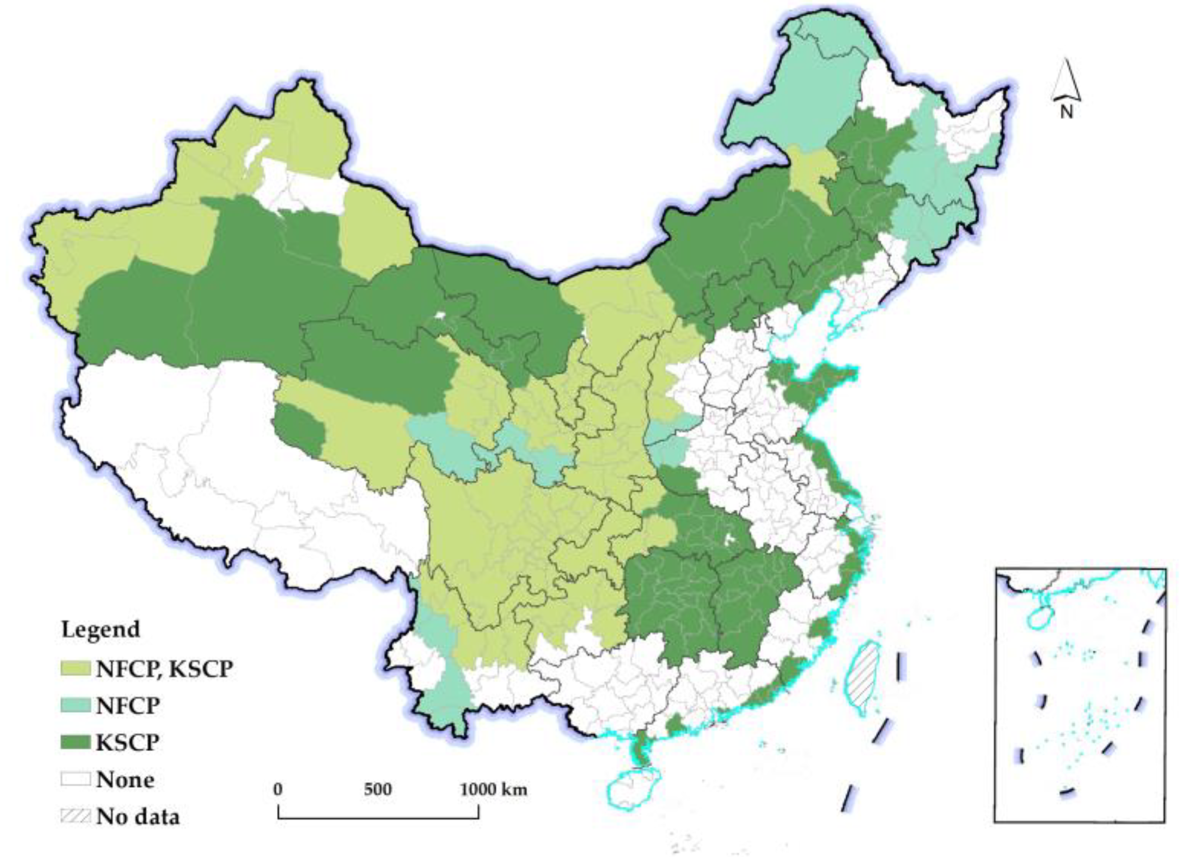
To improve the environmental quality and prevent windblown sand, the Chinese central government has implemented several national programs for forest conservation and construction. The Key Shelterbelt Construction Program (KSCP) and the Natural Forest Conservation Program (NFCP) are two important programs that cover a large scope and feature continuous implementation [23]. Therefore, we introduced two dummy variables to represent these programs, one for the units covered by the KSCP or NFCP program and the other units as a reference group.

2.4. Data Sources and Processing

We adopted land-use raster data with a resolution of 1 km × 1 km from 2000, 2010, and 2020; annual NDVI data with a resolution of 1 km × 1 km from 2000, 2010, and 2020; Digital Elevation Model data with a resolution of 30 m × 30 m, a spatial interpolation dataset of annual average temperature and precipitation, from 2000, 2010, and 2020; and land GDP data with a resolution of 1 km × 1 km from 2000, 2010, and 2019, supplied by the Data Center for Resources and Environmental Sciences, Chinese Academy of Sciences (RESDC) (https://www.resdc.cn, accessed on 10 July 2022).
Land-use data were employed to analyze land-use changes during the research period. The RESDC conducted image pre-processing, classification, and classification accuracy assessment of cloud-free Landsat Thematic Mapper (TM) (It was a whiskbroom instrument designed and built by SBRC (Santa Barbara Research Centre) of Hughes Aircraft Company in Goleta, USA) images with resolutions of 30 m and seven bands. Land-use types included (1) construction land, including urbanized, rural residential, and other construction land; (2) arable land; (3) woodland, including forestland, shrubland, open forestland, and other woodlands; (4) grassland, including high-, medium-, and low-coverage grassland; (5) water; and (6) unused land, including sand, bare land, bare rocky land, and others.
Annual NDVI data were generated using the maximum value of the monthly NDVI data. We adopted annual NDVI data to reflect the vegetation changes in the land-use patches. We employed land GDP data to calculate average rural land GDP. Specifically, based on the land-use data, we identified the rural scope by excluding urbanized land and then calculated the average value of the land GDP grids within the rural scope. The average temperature, precipitation, and terrain values of the grids within a research unit were calculated to represent the corresponding values of the research unit.
The population data in this study were primarily from the Population Census Data of China for 2000, 2010, and 2020, which provide information about the rural population at the prefectural level. Population data were employed to measure the rural population decline. Some research units have experienced administrative boundary adjustments; thus, we referred to the “Administrative Divisions Yearbook of China” from 2000 to 2020 to adjust the vector boundary and data to make them comparable over the years. Finally, the number of research units with comparable rural population data was 342 in the period 2000–2020 (Figure 2).
The data for the forest conservation and construction programs were from the Ministry of Ecology and Environment, which released a county list of the NFCP and KSCP programs. The prefectural units in which the listed counties are located were regarded as being covered by these programs (Figure 3).

3. Results

3.1. Rural Population Decline in China from 2000 to 2020

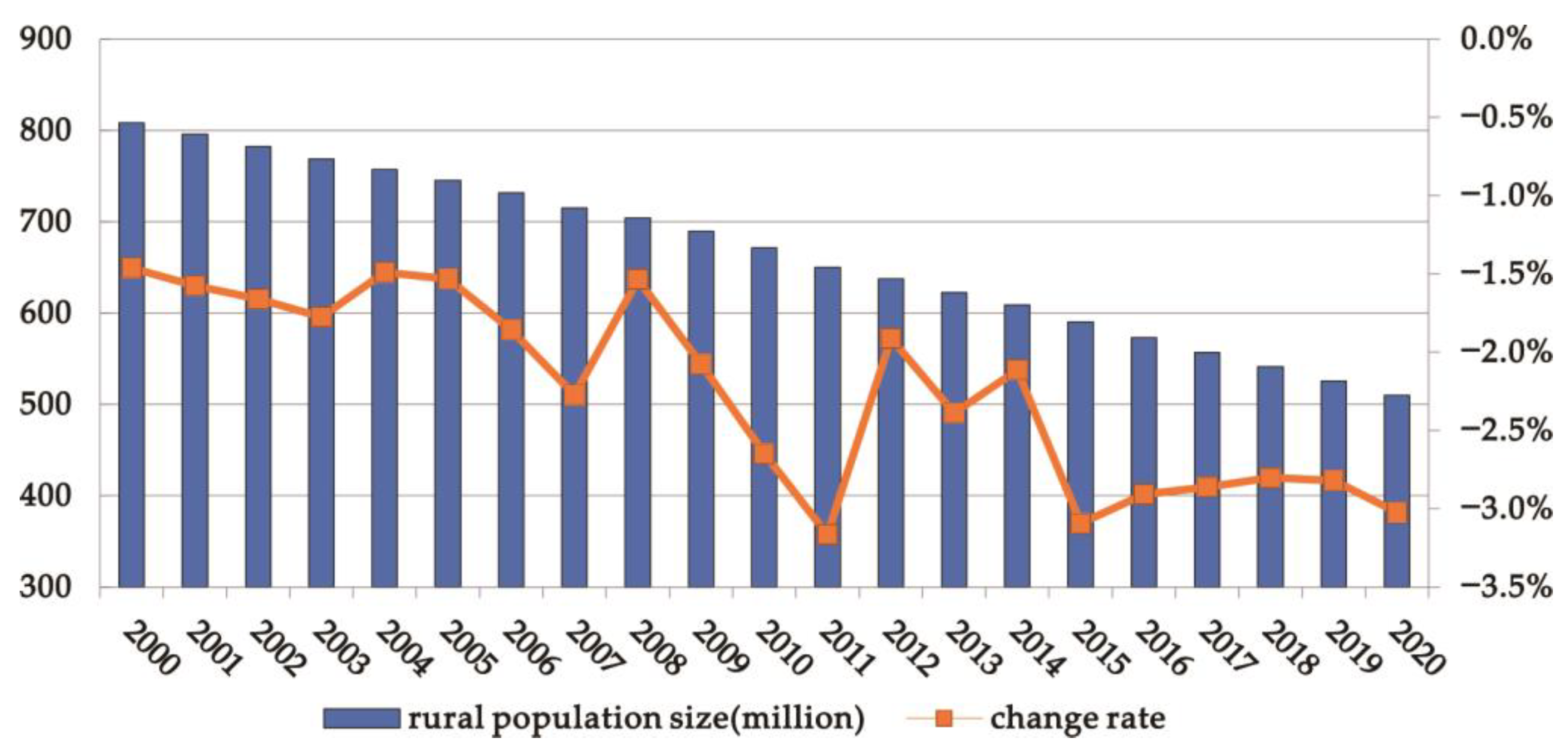
The rural population in China experienced a continuous decline from 2000 to 2020 (Figure 4). The size of the rural population declined from more than 800 million in 2000 to approximately 670 million in 2010, and then to approximately 500 million in 2020, with a total decline of approximately 37.5% from 2000 to 2020. The annual decline rate fluctuated but generally accelerated, increasing from approximately 1.5% in 2000 to approximately 2.5% in 2010 and then to approximately 3.0% in 2020. After 2015, this decreasing trend slowed but remained considerable.
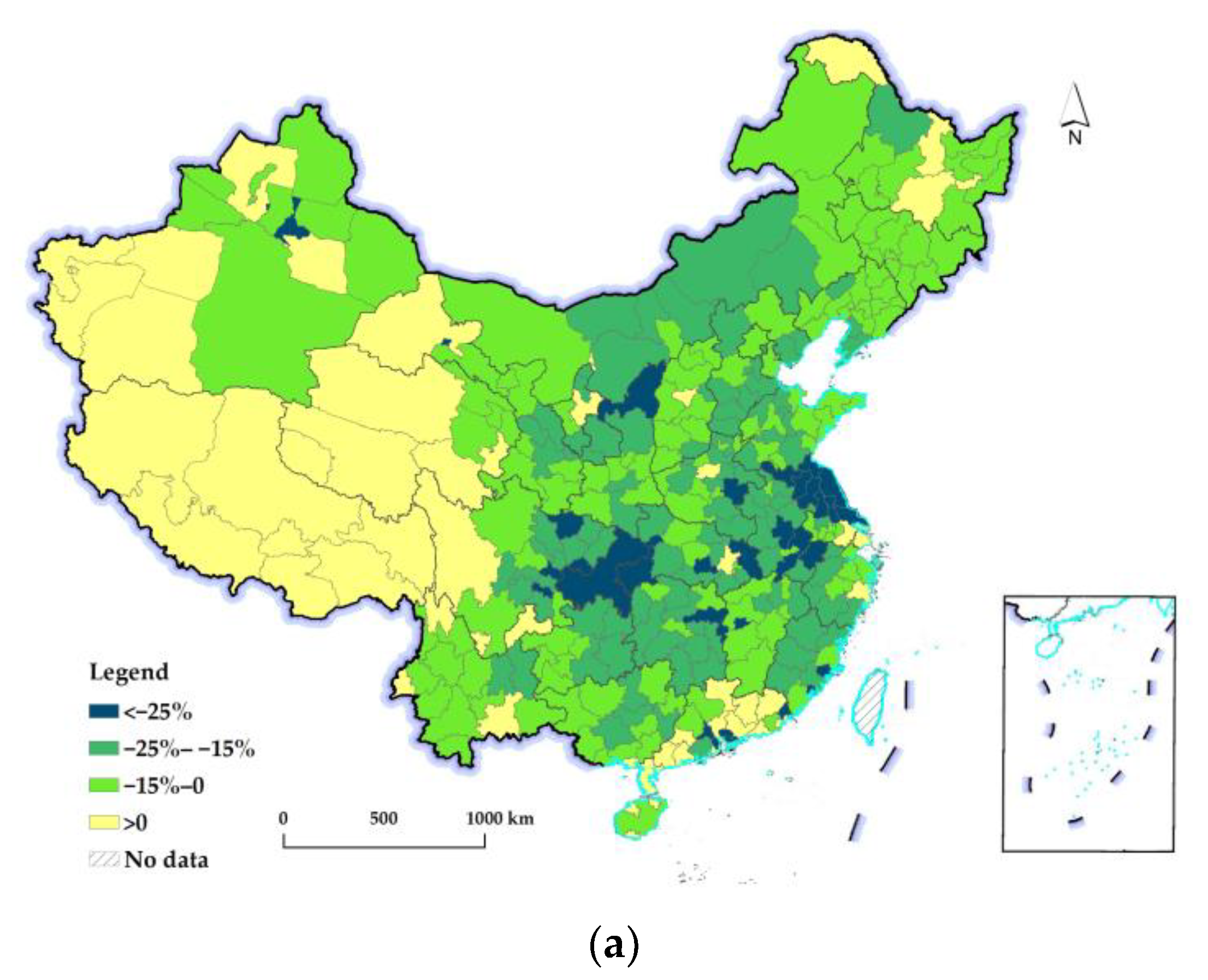
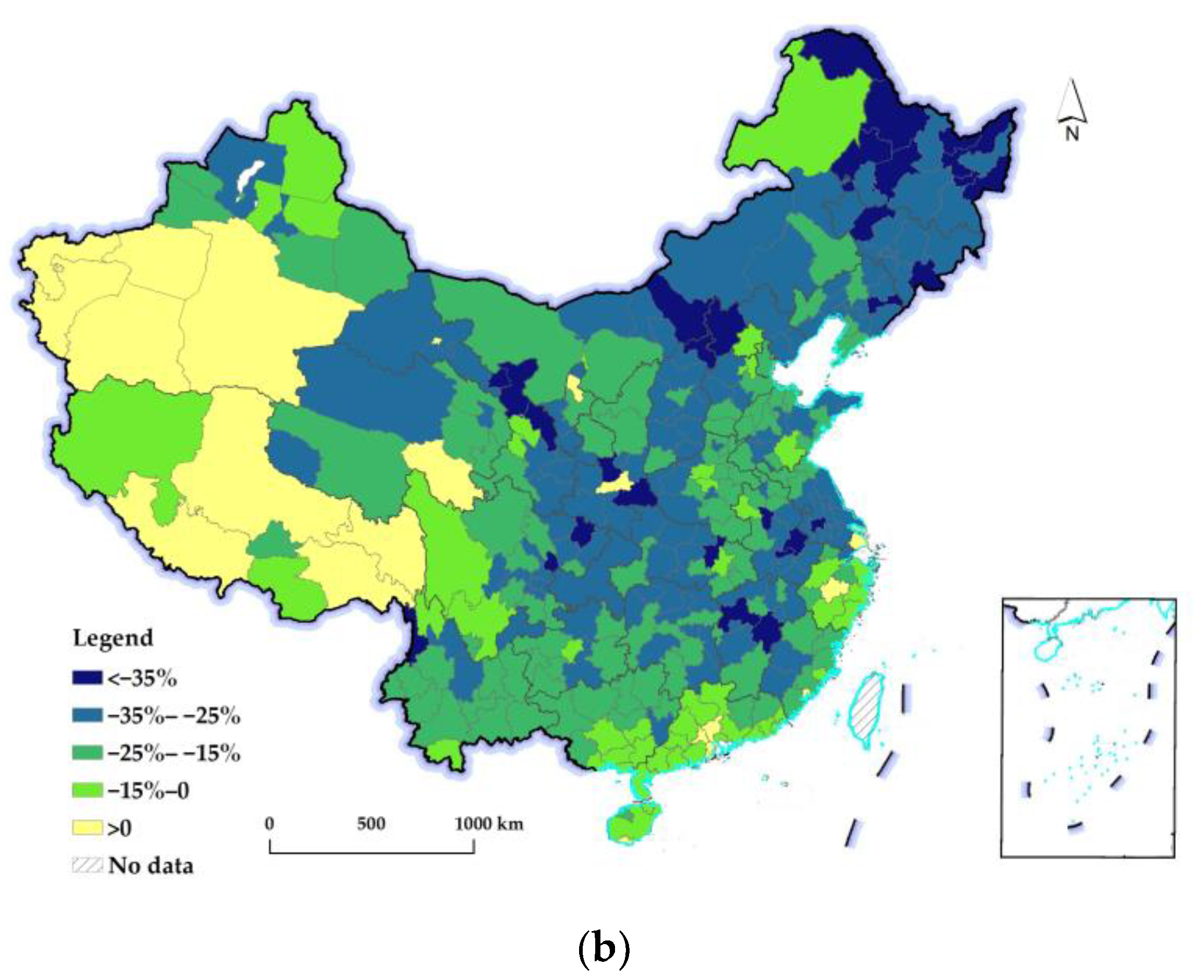
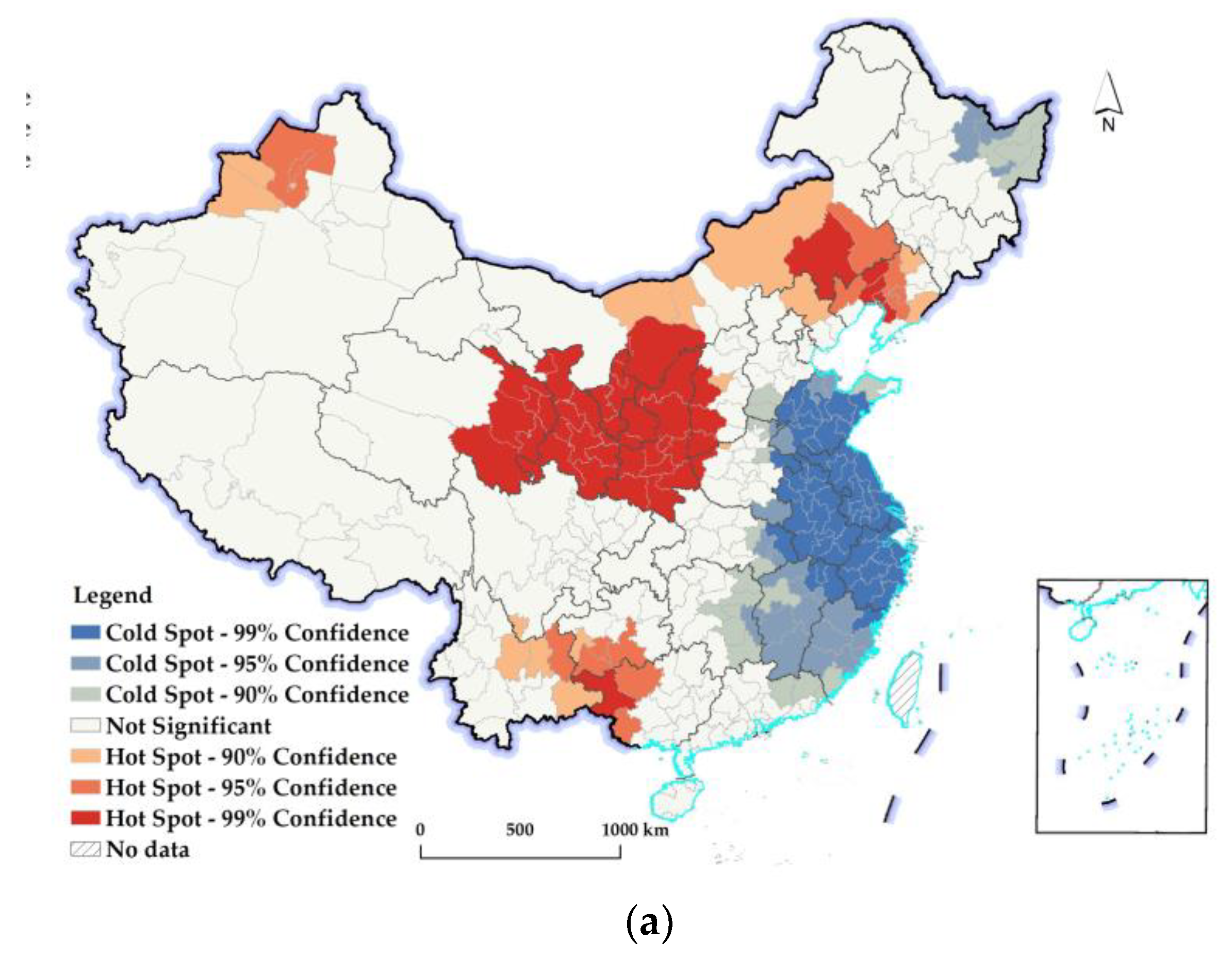
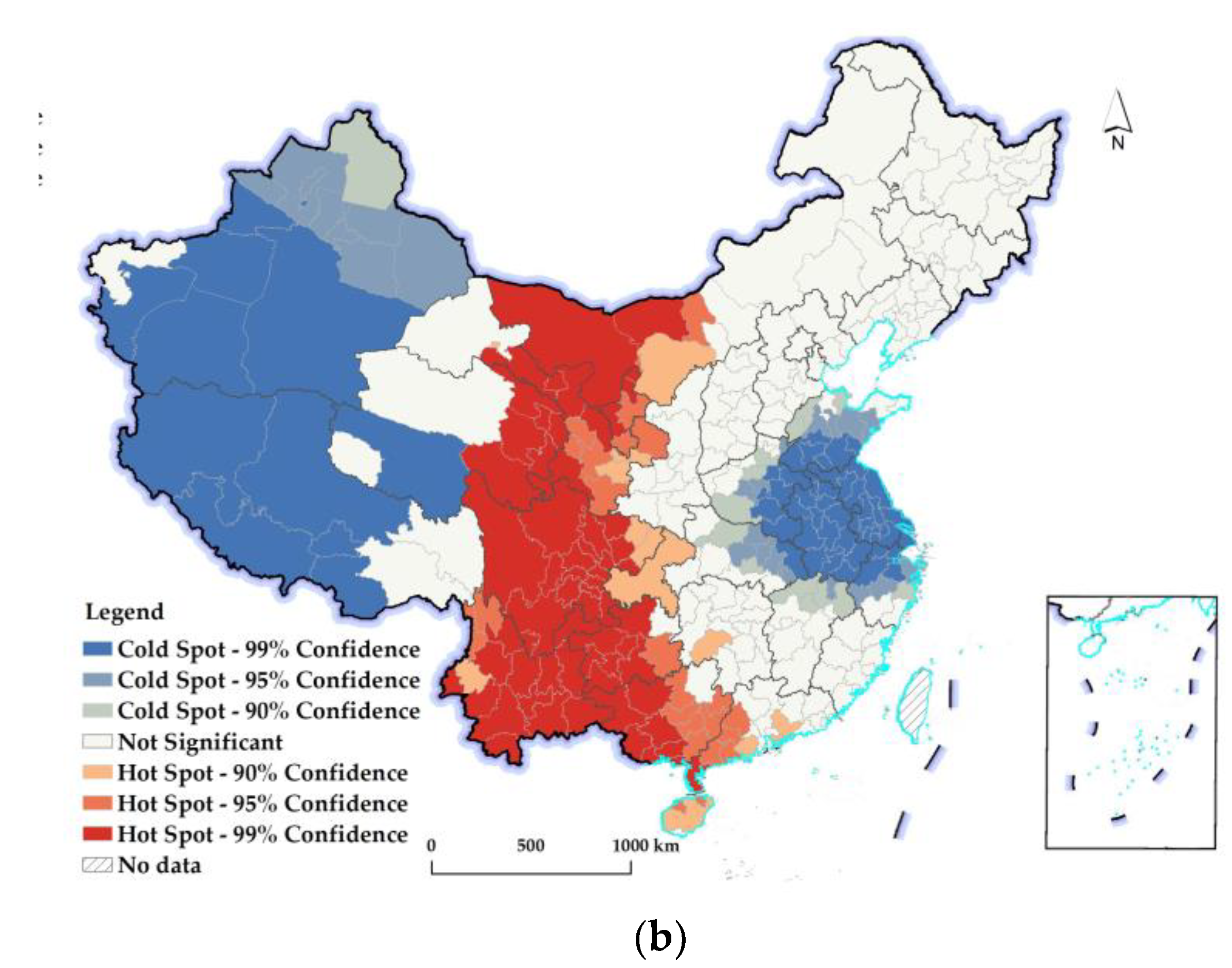
Most prefectural-level units also experienced significant rural population decline, with the average decline rates being approximately 16% and 24% during 2000–2010 and 2010–2020, respectively. Some spatial differences were also observed, as shown in Figure 5. First, the units with a severe rural population decline were concentrated in the following region from 2000 to 2010: (1) the peripheral area of the Yangtze River Delta (YRD), including Jiangsu, Zhejiang, and parts of Anhui, largely because the developed YRD region has attracted rural migrants from the surrounding areas; (2) the middle reaches of the Yangtze River region (MYR) and the Cheng-Yu region, which contains Hunan, Hubei, the northeast part of Sichuan, and Chongqing, which were characterized by the large rural population and less developed economy, with many rural migrants having moved to the coastal region to seek job opportunities; and (3) the northwest region, including central Inner Mongolia and northern Shaanxi, which has poor natural and production conditions. In contrast, the northeast and southwest regions had a relatively slight decline in the rural population, and Tibet, part of Xinjiang, and northern Guangdong, experienced a slight growth in the rural population, which may be closely related to their high natural growth rates.
Second, during 2010–2020, the units with a severe decline in rural population were still concentrated in the peripheral area of the YRD, MYR, Cheng-Yu, and northwest regions, and most of these units had a higher decline rate than those from 2000 to 2010. Moreover, the units in the Gansu, Shaanxi, Shanxi, Jiangxi, and northeast regions experienced a significant increase in the decline rate, whereas the units in Shandong, Zhejiang, Guangdong, and the southwest region had a relatively low decline rate, and some units in Tibet had a positive change in the rural population.
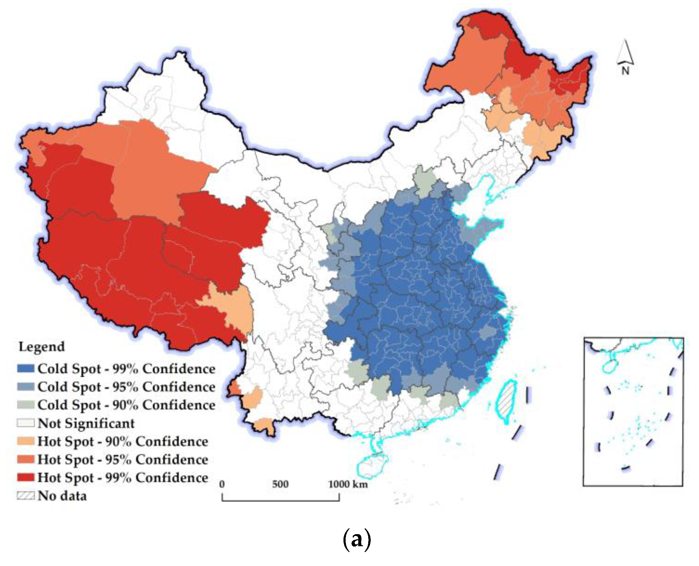
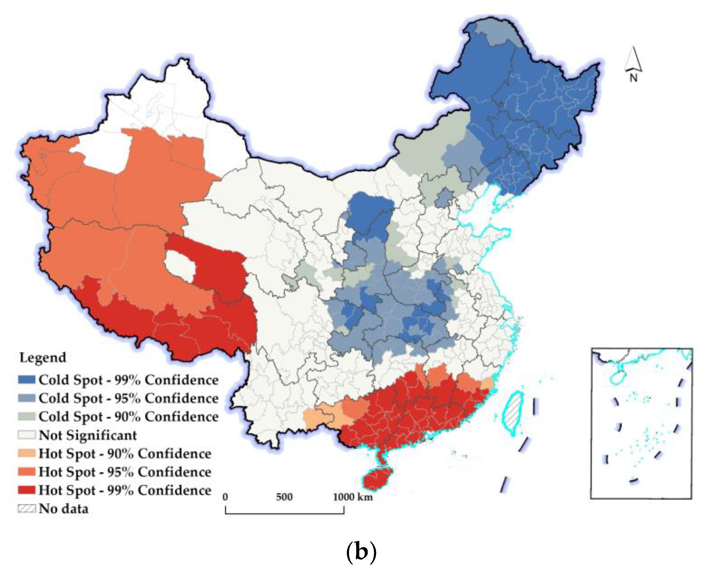
The results of the hot-spot analysis are presented in Figure 6. Most of the units in the coastal, central, and western regions formed cold spots from 2000 to 2010, indicating that these units had a significantly higher decline rate in the rural population. Meanwhile, the hotspots were concentrated in the northeast region, Tibet, and part of Qinghai. There were some changes from 2010 to 2020. The cold spots formed two concentration regions: one contained the units in the MYR, Cheng-Yu, and northwest regions, and the other mainly referred to the northeast region. In contrast, most units in coastal regions became insignificant. The units in Tibet were still hot spots, and most units in Guangdong, Guangxi, Fujian, and Jiangxi changed from insignificant to hot spots.

3.2. Spatiotemporal Differences of Changes in the REQ

3.2.1. An Overall Picture of the Change in the REQ at the National Level

The national REQ improved during both periods (2000–2010 and 2010–2020). The average values of the change in REQ at the national level were approximately 6.8% from 2000 to 2010 and approximately 2.0% from 2010 to 2020. This benefitted from the transformations between the subtype of grassland, the transformations from grassland to woodland, the returning or abandonment of arable land, and the transformations from unused lands to woodland and grassland (Table 3); however, some differences were observed between the two periods. The contributions of transformations related to unused and arable land increased, and those related to grassland and woodland declined significantly.
In contrast, some land-use changes reduced the REQ. The degradation of grassland, expansion of arable land, and degradation of woodland were the three most important reasons for REQ decline; however, the contribution of arable land expansion to the decline in REQ was reduced from 34.6% to 22.3%. The degradation of woodland increased its contribution to the decline in the REQ. Moreover, the percentage of the occupation of construction land to the total patches with declined EQ significantly increased from 2.8% in the first period to 10.6% in the second period.
Overall, the land-use changes that influenced the REQ were two coexisting processes. The decline in REQ caused the expansion of arable land to decline, and the return or abandonment of arable land contributed to the improvement of the REQ. The transformation of unused land to grassland and woodland, and the improvement of existing woodland and grassland, exceeded the reverse processes, which were significant contributors to the improvement in the REQ.

3.2.2. Spatiotemporal Differences in Changes in the REQ at the Prefectural Level

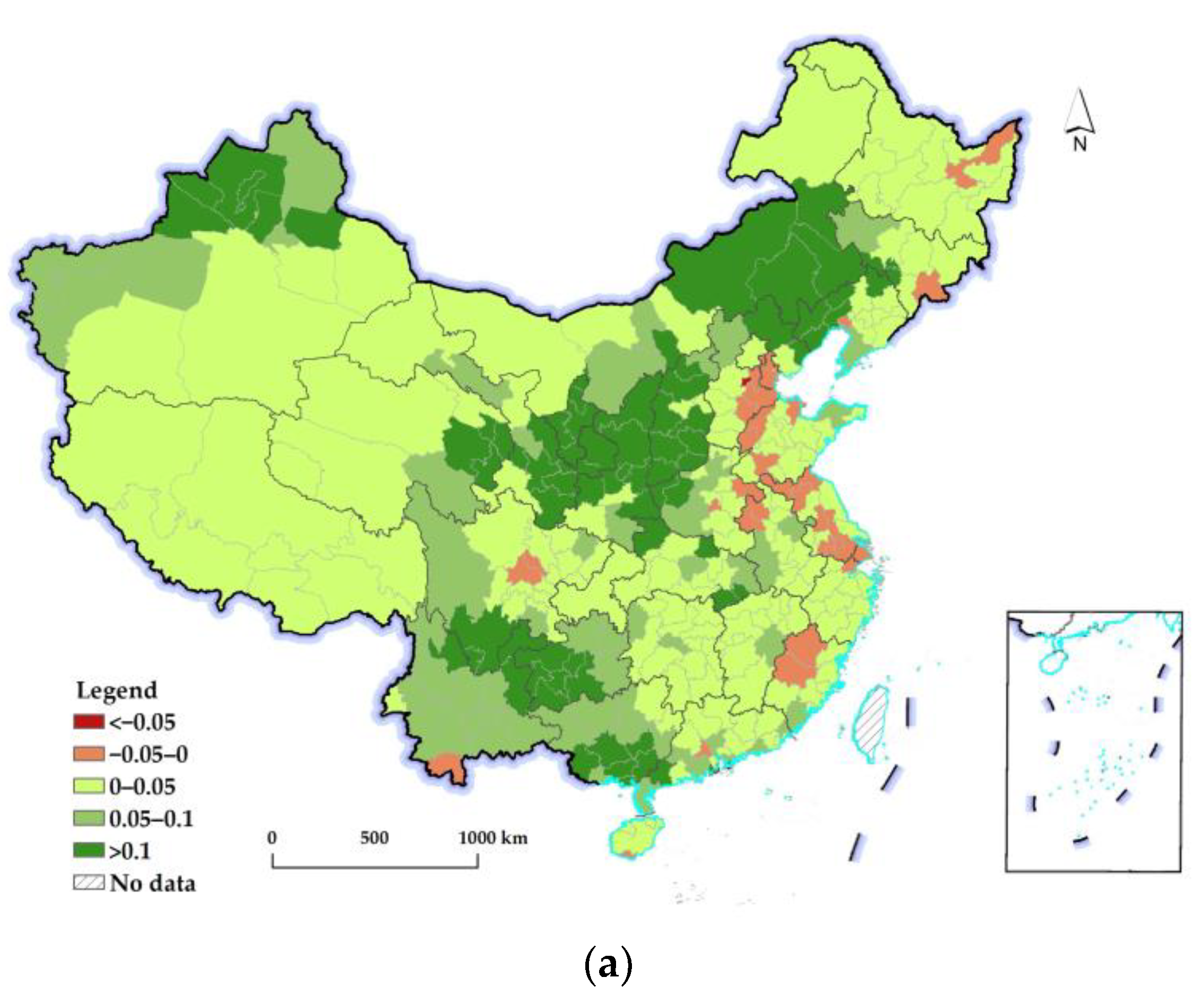
Approximately 9.2% of the research sample had a decline in REQ from 2000 to 2010, and it was mainly scattered in the coastal regions, including Hebei, Shandong, and Jiangsu. The units with a significant improvement in REQ were concentrated in the following regions (Figure 7): (1) the northwest region, including northern Shaanxi, Ningxia, Gansu, and the northeast part of Inner Mongolia, which are known as the fragile eco-environment but have gained considerable support from the central government to protect the grassland and forestland; (2) the southwest region, including Yunnan, Guizhou, Guangxi, and southern Sichuan, which are mountainous areas with relatively abundant precipitation; and (3) the border areas of Xinjiang, which are characterized by a fragile eco-environment and low population density.
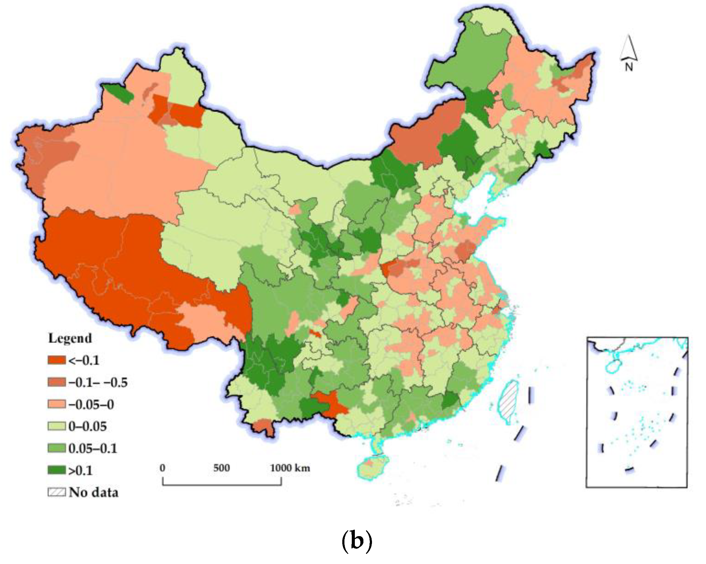
From 2010 to 2020, more than one-third of the research units had a declined REQ. The coastal region, especially Hebei, Shandong, and Jiangsu, experienced an obvious expansion of units with a declining REQ. Many units in the central region, especially those in Henan and Anhui, changed from a slight increase to a slight decrease in REQ. Some units in the northeast region, Tibet, and Xinjiang also experienced a slight decline in REQ. Units with a significantly increased REQ were still concentrated in the southwest and northwest regions. Moreover, many units in Guangdong, Guangxi, and parts of Fujian experienced significant improvements in the REQ.
Figure 8 presents the results of the hot-spot analysis. From 2000 to 2010, the cold spots were mainly concentrated in Shandong, Jiangsu, and Zhejiang in the coastal region and Anhui and Jiangxi in the central region. Hot spots were distributed in the northwestern and southwestern regions. From 2010 to 2020, the cold spots shrank, but they were still concentrated in Shandong and Jiangsu. Anhui, Henan, and Hubei in the central region and Tibet and Xinjiang in the western region experienced an increase in cold spots. In contrast, the hot spots significantly expanded in the western region, indicating that the REQ continuously improved during the research period.

3.3. Examining the Impacts of the Rural Population Decline on the Changes in the REQ

3.3.1. Results for All Samples

Table 4 presents the REQ variations for all samples. Multicollinearity problems were examined using the variance inflation factor (VIF). The models passed the collinearity threshold (VIF < 5 for the average value and that of each variable) and the Breusch–Pagan test for heteroscedasticity problems. The F statistics were all significant at a confidence level of 99% and the adjusted R2 values were greater than 0.45, showing good explanatory power for the changes in the REQ.
Rural population changes can significantly explain REQ variations during the two periods. The coefficients for the CRPD were significantly negative, suggesting that more serious rural population declines lead to greater REQ improvements. However, the absolute values of the coefficients for CRPD were significantly lower than those of most of the variables with a significant coefficient, such as temperature, precipitation, and RPD. This indicates that the influence of CRPD on the change in REQ was relatively low.
The rural population density, a control variable, significantly affected the change in the REQ. The coefficients for RPD were both significantly negative in the two periods, suggesting that a low rural population density can contribute to improving the REQ. Moreover, the absolute values of the coefficients for the RPD were relatively high, indicating that rural population density can largely determine the changes in the REQ.
Natural factors generally had a significant influence on REQ variations. The terrain had significantly positive coefficients, showing that units with higher terrain had more improved REQs. A possible reason may be that regions with a higher terrain generally have poor production conditions, which can help prevent intensive production activities. Temperature and precipitation also had significantly positive values, suggesting that the higher the temperature and precipitation, the higher the improvement in the REQ.
Economic variables had varied effects on changes in REQ. Rural land average GDP had trivial influences on the changes in REQ in the two periods, given that the coefficients for LGDP were insignificant. This may be because the rural economic activities in most units, especially those in the central and western regions, were relatively low during the research period. Furthermore, the growth of rural land average GDP had minimal influence on the changes in the REQ in the period from 2000 to 2010, but its influence became significant from 2010 to 2020. The higher the growth of the rural land average GDP, the more the REQ declined. The reason may be that many units have experienced rapid rural economic development supported by the rural revitalization strategy in recent decades, which has brought some pressure on the REQ. Road network density had a significant influence on the change in the REQ, with a high road network density reducing the REQ, possibly because a high road network density can extend human activities.
The coefficients for NFCP and KSCP were significantly positive, suggesting that the units covered by the programs on forest conservation improved more in the REQ. The absolute value of the coefficient for NFCP was higher than that of KSCP, implying that the NFCP program had a stronger influence on the improvement in the REQ, possibly because the implementation of the NFCP program was relatively easier.

3.3.2. Results for Different Regions

The performance of the variables in different regions, namely, the coastal, central, and western regions, was investigated. The coastal region is characterized by a high rural population density and developed rural economy, whereas the central region is characterized by a high rural population density but a less developed rural economy dominated by agricultural production. The western region generally has a relatively low rural population density, a less developed rural economy, and a fragile eco-environment.
Temperature and precipitation were highly correlated in the coastal and central regions, and the VIF values of temperature were higher than 5; thus, we excluded the temperature from the models for the coastal and central regions. Moreover, the NFCP program covered a small part of the coastal region; thus, it was not included in the models for the coastal region. The models passed the collinearity threshold and the F statistics, and the adjusted R2 values were approximately 0.4, showing good explanatory power for the changes in the REQ. This led to several interesting results (Table 5).
Rural population changes can significantly explain the changes in the REQ in the western region. The coefficients for CRPD were significantly negative, which was consistent with those of the models for all samples. The western region generally has a fragile eco-environment and the REQ may be sensitive to rural population changes. In contrast, rural population change had weak explanatory power for changes in the REQ in the coastal and central regions. This may be because units with a declined REQ in the coastal and central regions were the most populated areas, and the rural population decline may not have reached the threshold to significantly alleviate the human–environment tension. For example, the reclamation of arable land and construction of rural homesteads were still observed during the research period.
Economic factors had varied explanatory powers for changes in REQ in different regions. In the coastal region, the coefficients for LGDP and RLGDP were significantly negative in both periods, reflecting that the high intensities of economic activities prevented the improvement of REQ. In the central and western regions, the coefficients for LGDP were insignificant, possibly because their rural economic developments were at a low absolute level, which cannot sufficiently influence REQ variations; however, the coefficients for RLGDP were significantly negative in the central and western regions, suggesting that the growth of average rural land GDP reduced the REQ in some units.
From a comprehensive perspective, the REQ variations in the coastal region were determined by economic and natural factors, and state eco-environmental protection policies also played an important role. In contrast, demographic factors had relatively weak influences on the changes in the REQ. In the central region, rural population density was a leading factor in the changes in the REQ, and state policies were also very important for the improvement of the REQ, but economic factors had relatively weak influences on the changes in the REQ. In the western region, demographic, natural, and state policy factors had significant influences on changes in the REQ, and economic factors were increasingly important in affecting the REQ.

4. Discussion

Rural population decline and associated socioeconomic problems have attracted considerable attention from scholars and policymakers [4,5]; however, considering the tension in the human environment resulting from the large population size in rural Chinese areas, this study aimed to explore whether rural population decline could contribute to the improvement in the REQ. This may support policies for sustainable rural development of the eco-environment.

4.1. Performance Evaluation of the Revised EQI Method for Measuring Changes in the REQ

Many studies have adopted the EQI method to measure eco-environmental quality based on the eco-environmental quality values of different land-use types [30,31,32,33]. In this study, we revised the EQI method in several ways. First, we measured the percentage of the net number of patches with a decrease and an increase in the EQ to the total patches of a region, rather than calculating the specific eco-environmental values, to measure the changes in the REQ. This can avoid the possible different results caused by the evaluation of the absolute EQI values of different land-use types, and it makes the differences in REQ variations among regions more comparable. Second, we excluded the eco-environmental change caused by land-use transitions with little or no clear connection with rural population activities; thus, our estimation of the changes in the REQ was closely related to rural population activities. Third, we considered the EQ change of unchanged land by introducing the NDVI data, and the results showed that approximately 10% of unchanged land led to a significant change in the NDVI value. Therefore, our revised method may improve the measurement of eco-environmental changes related to rural population activities.
We cannot evaluate the accuracy of our results by comparing them with existing studies because few studies have directly explored the REQ change in China. Nevertheless, the following aspects may help confirm the validity of our results. First, existing studies have shown that many regions (containing urban and rural areas) in western China improved eco-environmental quality from 2000 to 2015 [32], indicating that the REQ in the western region may have also improved, which is consistent with our findings. Second, using Heilongjiang as a case, we found that most units in Heilongjiang had a declining REQ from 2010 to 2020. The research of Wang et al. (2020) revealed that the rural settlements expanded significantly from 2000 to 2020 [51], and declining NDVI values have also been observed in the past few decades [52], supporting that Heilongjiang may have experienced a reduced REQ in recent decades. Third, we found that many units in the coastal and central regions have reduced their REQ, which is consistent with the empirical knowledge, because the coastal region has a rapid industrial development and the central region has a quite high rural population density, which may prevent the improvement of the REQ.

4.2. REQ Changes and the Factors

Our results showed that the REQ at the national level improved in both periods (2000–2010 and 2010–2020). This is not consistent with studies on the eco-environmental change of a whole region, which have shown that eco-environmental quality has generally declined in recent decades [31,32]. This indicates that existing studies may not accurately reflect REQ variations, and the rapid expansion of urban land is the primary driver of the decline in eco-environmental quality. Moreover, we found that the changes in the REQ had significant spatial differences, which is similar to the findings of existing studies. Many units in the coastal and central regions led to a declined REQ, and many units in the western region had the opposite result.
Existing studies have revealed that eco-environmental changes are negatively related to population density, but the role of rural population decline remains unclear [20,32,35]. In this study, we also found that a low rural population density can promote REQ. More importantly, our empirical models verified that rural population decline can contribute to the improvement of the REQ; however, we also found that the absolute influence of rural population decline on changes in the REQ was lower than that of rural population density. Although many units have experienced significant rural population decline in past decades, the absolute size of the rural population is still substantial in many regions. Thus, the out-migration of the rural population may not have fundamentally changed the human–environment tension, which limited the contribution of rural population decline to REQ improvements.
We also found that rural population decline had varied influences on changes in the REQ among different regions. Rural population decline significantly improved the REQ in the western region characterized by a low rural population density and a fragile environment. However, the rural population decline had a weak influence on the REQ in the coastal and central regions. This may be because these regions have a large rural population and labor surpluses, the rural population decline may not have reached a threshold to produce enough influences on the REQ changes, and the remaining population in the rural areas still put significant pressure on the REQ. This may also be related to the natural conditions and local policies in these regions [20,22]. Thus, we argue that although rural population decline can generally promote the REQ, its impact on the changes in the REQ in a specific context may still need further examination.
The important role of eco-environmental protection programs in eco-environmental change has been addressed in previous studies [23,32]. Our results are consistent; that is, the NFCP and KSCP programs significantly promoted the REQ, especially in the western region. In contrast to existing findings, we found that economic factors did not strongly affect changes in REQ. This may be related to the fact that industrial development has been concentrated in urban areas and has been very weak in most rural areas.

4.3. Policy Implications

Our findings have several implications for sustainable development policies. First, we suggest that governments take a more comprehensive view of rural population decline. Policymakers have focused on the negative impact of rural population decline; however, the large rural population has put considerable pressure on the rural eco-environment, such as the occupation of ecological land and the destruction of vegetation. We found that rural population decline can generally alleviate human–natural tension and promote the REQ, and thus controlling rural populations can contribute to the sustainable development of the rural eco-environment, especially in areas with a fragile eco-environment. Second, economic growth in many rural areas has a significant negative influence on REQ; thus, we suggest that governments should pay attention to the eco-environmental effect of rural industrial development in a rural industrial revitalization context. For one thing, rural industrial development should conserve land and use it intensively; for another, it may need to control the development of industries with serious pollution. Third, environmental protection programs have significantly promoted the REQ. However, these programs have focused on the regions with a fragile eco-environment in the western region, and many populated regions in the coastal and central regions have not been covered. We suggest that the central government extend the coverage of these programs, especially in regions with a declining REQ.

5. Conclusions

Based on remote-sensing data, including land-use data and NDVI data, this study revised the EQI method to measure the changes in the REQ and built empirical models to explore the impacts of rural population decline on the changes in the REQ. We found that REQ improved nationally from 2000 to 2020, with some significant spatial differences; that is, the units with declining REQ were mainly concentrated in the coastal and central regions, and most units in the western region significantly promoted the REQ. Our empirical models revealed that the rapid decline in the rural population contributed to the improvement in the REQ. However, the influence of rural population decline on the changes in the REQ was closely related to the regional context and was more significant in the western region with a fragile environment. Moreover, whereas the rural population density and economic growth had negative effects on the changes in the REQ, the favorable natural factors and the state eco-environmental protection policies contributed to the improvement of the REQ. We suggest controlling the rural populations in the regions with a fragile eco-environment and a declining REQ, which can contribute to the sustainable development of the rural eco-environment.
This study contributes to existing research in the following aspects. First, we measured the EQ change targeted at rural areas and verified the positive influence of rural population decline on the changes in the REQ. This will contribute to the understanding of the positive aspects of rural population decline for the sustainable development of rural areas. Second, we proposed a revised EQI method that can be applied to measure changes in the REQ related to rural population activities. The revised EQI method can avoid the possible different results caused by the evaluation of the absolute EQI values of different land-use types, and it also considers the EQ change of the unchanged land-use patches.
Finally, this study has several limitations. First, the eco-environmental effects of rural population change are complex; the REQ change reflected by land-use change is only one of the aspects, and the exploration of other aspects may further deepen the understanding of the relationship between rural population activities and REQ changes. Second, the regional contexts in China are quite different, and the research at the national scale may not accurately reflect the relationship between rural population decline and REQ changes in some specific regions, especially the regions with complex human–natural relationships. Third, the mechanism of the influence of rural population decline on the changes in the REQ may need to be further explored from the perspective of rural household investigation or case studies.

Funding

This research was funded by the National Natural Science Foundation of China, grant No. 42001166, 42271246.

Data Availability Statement

Not applicable.

Conflicts of Interest

The author declares no conflict of interest.

References

  1. United Nations. World Urbanization Prospects—Population Division; United Nations: New York, NY, USA, 2019. [Google Scholar]
  2. Mukerji, S.; Gupta, R.B. Population Change and Economic Development in Rural India. Rele J. 2011, 30, 241–243. [Google Scholar]
  3. Anríquez, G.; Stloukal, L. Rural Population Change in Developing Countries: Lessons for Policymaking. Eur. View 2008, 7, 309–317. [Google Scholar] [CrossRef] [Green Version]
  4. Liu, Z.; Liu, S.; Jin, H.; Qi, W. Rural Population Change in China: Spatial Differences, Driving Forces and Policy Implications. J. Rural Stud. 2017, 51, 189–197. [Google Scholar] [CrossRef]
  5. Liu, Y.; Liu, Y. Progress and Prospect on the Study of Rural Hollowing in China. Geogr. Res. 2010, 29, 25–42. [Google Scholar]
  6. Qu, Y.; Long, H. The Economic and Environmental Effects of Land Use Transitions under Rapid Urbanization and the Implications for Land Use Management. Habitat Int. 2018, 82, 113–121. [Google Scholar] [CrossRef]
  7. Liu, Z. Rural Population Decline, Cultivated Land Expansion, and the Role of Land Transfers in the Farming-Pastoral Ecotone: A Case Study of Taibus, China. Land 2022, 11, 256. [Google Scholar] [CrossRef]
  8. He, S.; Shao, H.; Xian, W.; Yin, Z.; You, M.; Zhong, J.; Qi, J. Monitoring Cropland Abandonment in Hilly Areas with Sentinel-1 and Sentinel-2 Timeseries. Remote Sens. 2022, 14, 3806. [Google Scholar] [CrossRef]
  9. Wei, Z.; Gu, X.; Sun, Q.; Hu, X.; Gao, Y. Analysis of the Spatial and Temporal Pattern of Changes in Abandoned Farmland Based on Long Time Series of Remote Sensing Data. Remote Sens. 2021, 13, 2549. [Google Scholar] [CrossRef]
  10. He, W.; Yan, J.; Zhou, H.; Li, X. The Factors Influencing Rural Household Firewood Consumption: A Theoretical Model and Empirical Research of a Typical Area in Chongqing Municipality. Shengtai Xuebao 2016, 36, 1369–1379. [Google Scholar]
  11. Knight, K.W.; Rosa, E.A. Household Dynamics and Fuelwood Consumption in Developing Countries: A Cross-National Analysis. Popul. Environ. 2012, 33, 365–378. [Google Scholar] [CrossRef]
  12. Zheng, Z.; Wu, Z.; Chen, Y.; Yang, Z.; Marinello, F. Exploration of Eco-Environment and Urbanization Changes in Coastal Zones: A Case Study in China over the Past 20 Years. Ecol. Indic. 2020, 119, 106847. [Google Scholar] [CrossRef]
  13. McDonald, R.I.; Marcotullio, P.J.; Güneralp, B. Urbanization and Global Trends in Biodiversity and Ecosystem Services. In Urbanization, Biodiversity and Ecosystem Services: Challenges and Opportunities: A Global Assessment; Springer: Berlin/Heidelberg, Germany, 2013. [Google Scholar]
  14. Robson, J.P.; Berkes, F. Exploring Some of the Myths of Land Use Change: Can Rural to Urban Migration Drive Declines in Biodiversity? Glob. Environ. Change 2011, 21, 844–854. [Google Scholar] [CrossRef]
  15. Martínez-Zarzoso, I.; Bengochea-Morancho, A.; Morales-Lage, R. The Impact of Population on CO2 Emissions: Evidence from European Countries. Environ. Resour. Econ. 2007, 38, 497–512. [Google Scholar] [CrossRef]
  16. Hospers, G.-J.; Reverda, N. Managing Population Decline in Europe’s Urban and Rural Areas; Springer International Publishing: Cham, Switzerland, 2015. [Google Scholar]
  17. Gao, J.; Song, G.; Liu, S. Factors Influencing Farmers’ Willingness and Behavior Choices to Withdraw from Rural Homesteads in China. Growth Change 2022, 53, 112–131. [Google Scholar] [CrossRef]
  18. Gu, Z.; Zhang, Z.; Yang, J.; Wang, L. Quantifying the Influences of Driving Factors on Vegetation EVI Changes Using Structural Equation Model: A Case Study in Anhui Province, China. Remote Sens. 2022, 14, 4203. [Google Scholar] [CrossRef]
  19. Lü, Y.; Zhang, L.; Feng, X.; Zeng, Y.; Fu, B.; Yao, X.; Li, J.; Wu, B. Recent Ecological Transitions in China: Greening, Browning, and Influential Factors. Sci. Rep. 2015, 5, 8732. [Google Scholar] [CrossRef] [Green Version]
  20. Li, W.; Li, X.; Tan, M.; Wang, Y. Influences of Population Pressure Change on Vegetation Greenness in China’s Mountainous Areas. Ecol. Evol. 2017, 7, 9041–9053. [Google Scholar] [CrossRef]
  21. Costanza, R.; D’Arge, R.; de Groot, R.; Farber, S.; Grasso, M.; Hannon, B.; Limburg, K.; Naeem, S.; O’Neill, R.V.; Paruelo, J.; et al. The Value of the World’s Ecosystem Services and Natural Capital. Nature 1997, 387, 253–260. [Google Scholar]
  22. Lu, X.; Shi, Y.; Chen, C.; Yu, M. Monitoring Cropland Transition and Its Impact on Ecosystem Services Value in Developed Regions of China: A Case Study of Jiangsu Province. Land Use Policy 2017, 69, 25–40. [Google Scholar] [CrossRef]
  23. Li, G.; Fang, C.; Wang, S. Exploring Spatiotemporal Changes in Ecosystem-Service Values and Hotspots in China. Sci. Total Environ. 2016, 545–546, 609–620. [Google Scholar]
  24. Xiao, X.; Hu, M.; Tan, M.; Li, X.; Li, W. Changes in the Ecological Footprint of Rural Populations in the Taihang Mountains, China. Sustainability 2018, 10, 3741. [Google Scholar]
  25. Hao, H.; Zhang, J.; Li, X.; Zhang, H.; Zhang, Q. Impact of Livelihood Diversification of Rural Households on Their Ecological Footprint in Agro-Pastoral Areas of Northern China. J. Arid Land 2015, 7, 653–664. [Google Scholar] [CrossRef] [Green Version]
  26. Shan, Y.; Dai, X.; Li, W.; Yang, Z.; Wang, Y.; Qu, G.; Liu, W.; Ren, J.; Li, C.; Liang, S.; et al. Detecting Spatial-Temporal Changes of Urban Environment Quality by Remote Sensing-Based Ecological Indices: A Case Study in Panzhihua City, Sichuan Province, China. Remote Sens. 2022, 14, 4137. [Google Scholar] [CrossRef]
  27. Zhang, H.; Wang, T.; Ding, Z.; Zhang, X.; Han, L. Uncertainty Analysis of Impact Factors of Eco-Environmental Vulnerability Based on Cloud Theory. Ecol. Indic. 2020, 110, 105864. [Google Scholar] [CrossRef]
  28. Shao, H.; Sun, X.; Wang, H.; Zhang, X.; Xiang, Z.; Tan, R.; Chen, X.; Xian, W.; Qi, J. A Method to the Impact Assessment of the Returning Grazing Land to Grassland Project on Regional Eco-Environmental Vulnerability. Environ. Impact Assess. Rev. 2016, 56, 155–167. [Google Scholar] [CrossRef]
  29. Li, L.; Shi, Z.H.; Yin, W.; Zhu, D.; Ng, S.L.; Cai, C.F.; Lei, A.L. A Fuzzy Analytic Hierarchy Process (FAHP) Approach to Eco-Environmental Vulnerability Assessment for the Danjiangkou Reservoir Area, China. Ecol. Model. 2009, 220, 3439–3447. [Google Scholar] [CrossRef]
  30. Jiang, X.; Zhai, S.; Liu, H.; Chen, J.; Zhu, Y.; Wang, Z. Multi-Scenario Simulation of Production-Living-Ecological Space and Ecological Effects Based on Shared Socioeconomic Pathways in Zhengzhou, China. Ecol. Indic. 2022, 137, 108750. [Google Scholar] [CrossRef]
  31. Yang, Y.; Bao, W.; Li, Y.; Wang, Y.; Chen, Z. Land Use Transition and Its Eco-Environmental Effects in the Beijing-Tianjin-Hebei Urban Agglomeration: A Production-Living-Ecological Perspective. Land 2020, 9, 285. [Google Scholar] [CrossRef]
  32. Chen, W.; Li, J.; Zeng, J.; Ran, D.; Yang, B. Spatial Heterogeneity and Formation Mechanism of Eco-Environmental Effect of Land Use Change in China. Geogr. Res. 2019, 38, 2173–2187. [Google Scholar]
  33. Pang, R.; Hu, N.; Zhou, J.; Sun, D.; Ye, H. Study on Eco-Environmental Effects of Land-Use Transitions and Their Influencing Factors in the Central and Southern Liaoning Urban Agglomeration: A Production-Living-Ecological Perspective. Land 2022, 11, 937. [Google Scholar]
  34. Chen, W.; Chi, G.; Li, J. The Spatial Association of Ecosystem Services with Land Use and Land Cover Change at the County Level in China, 1995–2015. Sci. Total Environ. 2019, 669, 459–470. [Google Scholar] [CrossRef] [PubMed]
  35. Wang, L.; Yu, B.; Chen, F.; Wang, N.; Li, C. An Analysis of Eco-Environmental Changes in Rural Areas in China Based on Sustainability Indicators between 2000 and 2015. Land 2022, 11, 1321. [Google Scholar] [CrossRef]
  36. Wang, M.; Qin, K.; Jia, Y.; Yuan, X.; Yang, S. Land Use Transition and Eco-Environmental Effects in Karst Mountain Area Based on Production-Living-Ecological Space: A Case Study of Longlin Multinational Autonomous County, Southwest China. Int. J. Environ. Res. Public Health 2022, 19, 7587. [Google Scholar] [CrossRef] [PubMed]
  37. Feng, S.; Fan, F. Developing an Enhanced Ecological Evaluation Index (EEEI) Based on Remotely Sensed Data and Assessing Spatiotemporal Ecological Quality in Guangdong-Hong Kong-Macau Greater Bay Area, China. Remote Sens. 2022, 14, 2852. [Google Scholar] [CrossRef]
  38. Shi, F.; Liu, M.; Qiu, J.; Zhang, Y.; Su, H.; Mao, X.; Li, X.; Fan, J.; Chen, J.; Lv, Y.; et al. Assessing Land Cover and Ecological Quality Changes in the Forest-Steppe Ecotone of the Greater Khingan Mountains, Northeast China, from Landsat and MODIS Observations from 2000 to 2018. Remote Sens. 2022, 14, 725. [Google Scholar] [CrossRef]
  39. Sun, R.; Wu, Z.; Chen, B.; Yang, C.; Qi, D.; Lan, G.; Fraedrich, K. Effects of Land-Use Change on Eco-Environmental Quality in Hainan Island, China. Ecol. Indic. 2020, 109, 105777. [Google Scholar] [CrossRef]
  40. Du, X.; Huang, Z. Ecological and Environmental Effects of Land Use Change in Rapid Urbanization: The Case of Hangzhou, China. Ecol. Indic. 2017, 81, 243–251. [Google Scholar] [CrossRef]
  41. Chen, D.; Lu, X.; Liu, X.; Wang, X. Measurement of the Eco-Environmental Effects of Urban Sprawl: Theoretical Mechanism and Spatiotemporal Differentiation. Ecol. Indic. 2019, 105, 6–15. [Google Scholar] [CrossRef]
  42. Asabere, S.B.; Acheampong, R.A.; Ashiagbor, G.; Beckers, S.C.; Keck, M.; Erasmi, S.; Schanze, J.; Sauer, D. Urbanization, Land Use Transformation and Spatio-Environmental Impacts: Analyses of Trends and Implications in Major Metropolitan Regions of Ghana. Land Use Policy 2020, 96, 104707. [Google Scholar] [CrossRef]
  43. Quintas-Soriano, C.; Castro, A.J.; Castro, H.; García-Llorente, M. Impacts of Land Use Change on Ecosystem Services and Implications for Human Well-Being in Spanish Drylands. Land Use Policy 2016, 54, 534–548. [Google Scholar] [CrossRef]
  44. Lawler, J.J.; Lewis, D.J.; Nelson, E.; Plantinga, A.J.; Polasky, S.; Withey, J.C.; Helmers, D.P.; Martinuzzi, S.; Penningtonh, D.; Radeloff, V.C. Projected Land-Use Change Impacts on Ecosystem Services in the United States. Proc. Natl. Acad. Sci. USA 2014, 111, 7492–7497. [Google Scholar] [CrossRef] [PubMed] [Green Version]
  45. Nuissl, H.; Haase, D.; Lanzendorf, M.; Wittmer, H. Environmental Impact Assessment of Urban Land Use Transitions—A Context-Sensitive Approach. Land Use Policy 2009, 26, 414–424. [Google Scholar] [CrossRef]
  46. Turner, B.L.; Lambin, E.F.; Reenberg, A. The Emergence of Land Change Science for Global Environmental Change and Sustainability. Proc. Natl. Acad. Sci. USA 2007, 104, 20666–20671. [Google Scholar] [CrossRef] [PubMed] [Green Version]
  47. Xu, D.; Deng, X.; Guo, S.; Liu, S. Labor Migration and Farmland Abandonment in Rural China: Empirical Results and Policy Implications. J. Environ. Manag. 2019, 232, 738–750. [Google Scholar] [CrossRef]
  48. Walters, B.B. Migration, Land Use and Forest Change in St. Lucia, West Indies. Land Use Policy 2016, 51, 290–300. [Google Scholar] [CrossRef]
  49. Grau, H.R.; Aide, T.M. Are Rural-Urban Migration and Sustainable Development Compatible in Mountain Systems? Mt. Res. Dev. 2007, 27, 119–123. [Google Scholar] [CrossRef] [Green Version]
  50. Xie, D.; Bai, C.; Wang, H.; Xue, Q. The Land System and the Rise and Fall of China’s Rural Industrialization: Based on the Perspective of Institutional Change of Rural Collective Construction Land. Land 2022, 11, 960. [Google Scholar] [CrossRef]
  51. Wang, J.; Wang, X.; Du, G.; Zhang, H. Temporal and Spatial Changes of Rural Settlements and Their Influencing Factors in Northeast China from 2000 to 2020. Land 2022, 11, 1640. [Google Scholar] [CrossRef]
  52. Chang, J.; Liu, Q.; Wang, S.; Huang, C. Vegetation Dynamics and Their Influencing Factors in China from 1998 to 2019. Remote Sens. 2022, 14, 3390. [Google Scholar] [CrossRef]
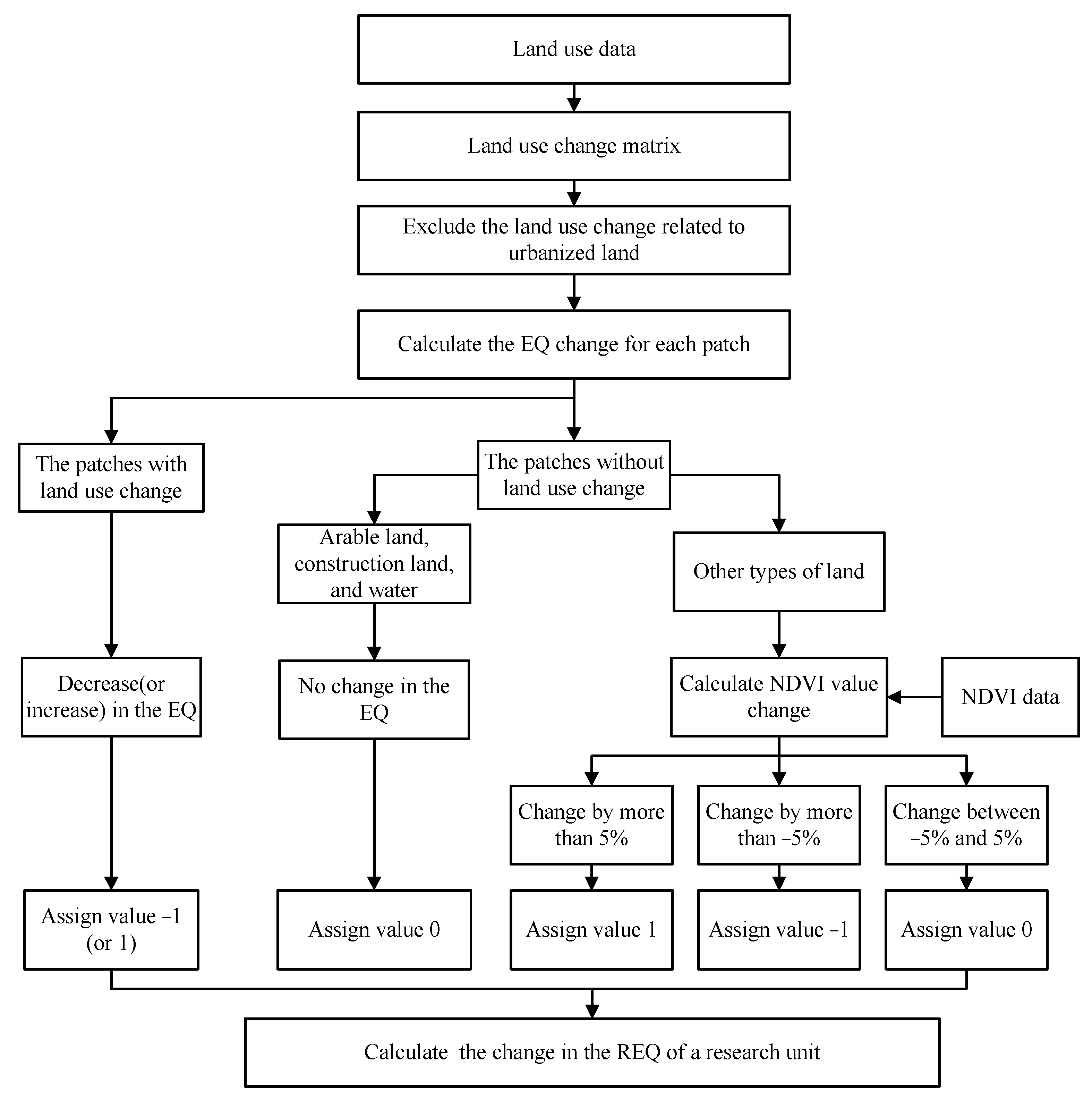
Figure 1. The main steps of measuring the change in the REQ.
Remotesensing 14 05217 g001
Figure 2. The research samples in this study.
Remotesensing 14 05217 g002
Figure 3. The spatial distribution of the NFCP and KSCP.
Remotesensing 14 05217 g003
Figure 4. Rural population change at the national level from 2000 to 2020.
Remotesensing 14 05217 g004
Figure 5. The changes in rural population density from 2000 to 2020. (a) 2000–2010; (b) 2010–2020.
Remotesensing 14 05217 g005aRemotesensing 14 05217 g005b
Figure 6. The hot spots of change in rural population density from 2000 to 2020. (a) 2000–2010; (b) 2010–2020.
Remotesensing 14 05217 g006aRemotesensing 14 05217 g006b
Figure 7. The changes in the REQ from 2000 to 2020. (a) 2000–2010; (b) 2010–2020.
Remotesensing 14 05217 g007aRemotesensing 14 05217 g007b
Figure 8. The hot spots of change in the REQ from 2000 to 2020. (a) 2000–2010; (b) 2010–2020.
Remotesensing 14 05217 g008aRemotesensing 14 05217 g008b
Table 1. The environmental-quality change among the transformation of different land-use types.
Land TypeArable LandForestlandShrublandOpen WoodlandOther WoodlandHC GrasslandMC GrasslandLC GrasslandWaterConstruction LandUnused Land
Arable landN
ForestlandDA
ShrublandDGA
Open woodlandDGGA
Other woodlandDGGGA
HC grasslandDGDDDA
MC grasslandDGGNDGA
LC grasslandDGGGGGGA
WaterDNNNNNNNN
Construction landGGGGGGGGGN
Unused landGGGGGGGGGDA
Note 1: HC, MC, and LC grasslands represent high-coverage, medium-coverage, and low-coverage grasslands, respectively. Note 2: The column is the initial land-use type, and the row is the land-use type at the end of the period. Note 3: N, D, and G indicate no change, a decrease, and a growth in the EQI, respectively, and A indicates that the results depend on the changes in the NDVI value.
Table 2. The variables and descriptions.
CategoriesVariablesDefinition and DescriptionAbbreviation
NaturalTerrainThe average terrain of a research unitTerrain
TemperatureThe average annual temperature during a certain periodTemp
PrecipitationThe average annual precipitation during a certain periodPrecipitation
EconomicRural land average GDP The average GDP value within the rural scope of a unitLGDP
Change in the rural land average GDPThe change rate of the rural land average GDPRLGDP
Road network densityThe ratio between the total mileage of the main road and the area in a research unitRND
DemographicRural population densityThe ratio between the number of the rural population and the area in a research unitRPD
Rural population density changeThe change rate of the rural population densityCRPD
State policyForest conservationThe Natural Forest Conservation ProgramNFCP
Forest constructionThe Key Shelterbelt Construction ProgramKSCP
Table 3. The land-use change matrix for the change in the REQ.
Arable LandWoodlandGrasslandWaterConstruction Unused LandTotal
The land-use change matrix for the improvement in the REQ (%)
Arable land0 (0)9.6 (12.0)8.7 (12.0)7.2 (8.2)0 (0)0 (0)25.5 (32.2)
Woodland0 (0)16.4 (4.7)1.1 (2.5)0 (0)0 (0)0 (0)17.5 (7.1)
Grassland0 (0)5.7 (7.2)26.6 (7.9)0 (0)0 (0)0 (0)32.3 (15.1)
Construction5.8 (2.3)0.1 (1.4)0.1 (1.8)0.2 (1.2)0 (0)0 (0.2)6.3 (6.8)
Unused land7.9 (4.9)0.9 (6.3)7.5 (19.0)1.6 (4.9)0 (0)0.5 (3.6)18.5 (38.7)
Total13.7 (7.2)32.6 (31.6)44.0 (43.1)9.0 (14.3)0 (0)0.6 (3.8)100 (100)
The land-use change matrix for the decline in the REQ (%)
Arable land0 (0)0 (0)4.3 (0)0 (0)0 (4.6)2.4 (3.9)6.6 (8.5)
Woodland7.8 (7.1)8.6 (5.7)4.8 (8.3)0 (0)0.9 (1.8)1.2 (4.9)23.3 (27.7)
Grassland19.5 (7.8)6.7 (4.2)14.5 (10.0)0 (0)0.9 (2.3)15.0 (20.7)56.7 (44.9)
Water7.3 (7.4)0 (0)0 (0)0 (0)1.0 (1.6)4.4 (5.6)12.6 (14.6)
Unused land0 (0)0 (0)0 (0)0 (0)0 (0.2)0.7 (4.1)0.8 (4.3)
Total34.6 (22.3)15.3 (9.8)23.6 (18.3)0 (0)2.8 (10.6)23.7 (39.1)100 (100)
Note 1: The values in brackets are those for 2010–2020. Note 2: The column is the initial land-use type, and the row is the land-use type at the end of the period. Note 3: The transformation between the same land-use type means there are changes among the subtypes or changes in the NVDI values.
Table 4. The regression results for all samples.
CategoriesVariables2000–20102010–2020
NaturalTerrain0.220 ***0.229 ***
Temp0.388 ***0.325 ***
Precipitation0.408 ***0.266 **
EconomicLGDP−0.112−0.120
RLGDP−0.027−0.133 ***
RND−0.156 **−0.097 **
DemographicRPD−0.309 ***−0.231 ***
CRPD−0.126 **−0.143 ***
State policyNFCP0.161 ***0.315 ***
KSCP0.134 ***0.141 **
Constant0.255 ***0.086 ***
F-value11.3911.69
Adjusted R20.470.52
Sample340340
Note 1: *** and ** denote significance at the 1% and 5% levels, respectively. Note 2: We have adopted the standardized coefficients for each variable.
Table 5. The regression results for different regions.
CategoriesVariablesCoastal RegionCentral RegionWestern Region
2000–20102010–20202000–20102010–20202000–20102010–2020
NaturalTerrain0.023 **0.255 **−0.0950.6510.253 ***0.176 **
Temp 0.475 ***0.215 **
Precipitation0.106 **0.187 **0.268 **0.1620.1180.340 ***
EconomicLGDP−0.099 **−0.227 **−0.088−0.150−0.331−0.326
RLGDP−0.014 **−0.065 **0.170−0.072 **−0.092 **−0.236 **
RND−0.017 **−0.071 **−0.101 **−0.112 **−0.276 ***−0.299 ***
DemographicRPD−0.145−0.083−0.586 **−0.297 **−0.446 ***−0.350 **
CRPD−0.054−0.152−0.057−0.053−0.205 **−0.160 **
State policyNFCP 0.230 **0.203 **0.1010.326 **
KSCP0.342 ***0.144 **0.0240.349 **0.283 ***0.239 ***
Constant0.029 ***0.042 ***0.560 ***0.931 ***1.344 ***1.511 ***
F-value9.5310.5616.2517.0116.5815.76
Adjusted R20.390.380.490.490.440.41
Sample90908383133133
Note 1: *** and ** denote significance at the 1% and 5% levels, respectively. Note 2: We have adopted the standardized coefficients for each variable. Note 3: The northeast region has not been analyzed because it contains only 36 research samples, which may affect the robustness of the regression results.
Publisher’s Note: MDPI stays neutral with regard to jurisdictional claims in published maps and institutional affiliations.