Biases Analysis and Calibration of ICESat-2/ATLAS Data Based on Crossover Adjustment Method

Abstract

The new-generation photon-counting laser altimeter aboard the Ice, Cloud, and Land Elevation Satellite-2 (ICESat-2) has acquired unprecedented high-density laser data on the global surface. The continuous analysis and calibration of potential systematic biases in laser data are important for generating highly accurate data products. Current studies mainly calibrate the absolute systematic bias of laser altimeters based on external reference data. There are few studies that focus on the analysis and calibration of relative systematic biases in long-term laser data. This paper explores a method for systematic biases analysis and calibration of ICESat-2 laser data based on track crossovers for the first time. In the experiment, the simulated data and ICESat-2 data were used to verify the algorithm. The results show that, during the three-year period in orbit, the standard deviation (STD) and bias of the crossover differences of the ICESat-2 terrain data were 0.82 m and −0.03 m, respectively. The simulation validation well demonstrate that the crossover adjustment can calibrate the relative bias between different beams. For ICESat-2 data, the STD of the estimated systematic bias after crossover adjustment was 0.09 m, and the mean absolute error (MAE) was 0.07 m. Compared with airborne lidar data, the bias and root mean square error (RMSE) of the ICESat-2 data remained basically unchanged after adjustment, i.e., −0.04 m and 0.38 m, respectively. This shows that the current ICESat-2 data products possess excellent internal and external accuracy. This study shows the potential of crossover for evaluating and calibrating the accuracy of spaceborne photon-counting laser altimeter data products, in terms of providing a technical approach to generate global/regional high-accuracy point cloud data with consistent accuracy.

1. Introduction

The spaceborne laser altimeter, as an important Earth observation instrument, has been widely used in ice sheet monitoring, canopy measurement, inland water monitoring, and ocean and land topographic mapping [1,2,3,4,5]. The instrument has demonstrated unprecedented height measurement accuracy. The agreement between the ICESat-2 data product and airborne laser data was high [6,7], with ground elevation bias of 0.18 m and canopy height bias of −1.71 m [8]. The accuracy of elevation control points obtained from the Ice, Cloud, and Land Elevation Satellite-2 (ICESat-2) laser data was better than 0.4 m, 0.6 m, and 1.0 m in flat, hilly and mountainous areas, respectively [9,10]. The elevation accuracy of radar-derived Digital Elevation Model (DEM) corrected by ICESat-2 laser data was improved by nearly 50% [11]. It is important to continuously calibrate and validate laser data to eliminate or reduce uncertainties and to better provide high-precision products to the research community. A variety of in-orbit geometric calibration methods for laser altimeters have been proposed, including the scanning maneuver method, the ground detector method, and the terrain matching method [12]. The scanning maneuver method uses the ranging residuals (the difference between the measured data and the data calculated based on the ranging model) in spaceborne laser scanning data to estimate the pointing and ranging system bias [13,14]. The ICESat and the ICESat-2 official mission teams have used scanning maneuvers on the ocean surface to achieve sub-arcsecond calibration of system pointing angle errors [15,16]. The ground detector method is a relatively direct calibration method. By laying a certain number of laser detector arrays with known positions in the calibration site, the captured satellite laser spot is positioned at the center of mass to calibrate the system pointing error [17,18]. The selection of the ground calibration site and the high cost restrict the wide adoption of this method. It will be difficult to apply this method to laser altimeters with thousands of beams in the future. The terrain matching method matches the known ground truth profile with the observation profile of the laser altimeter to estimate the system bias [19,20,21,22].

Unlike the above calibration methods, which require external reference data, the advantage of crossover analysis is that no a priori knowledge of the planet’s surface elevations is required; it only exploits consistency conditions that should be met at these crossovers [12]. Therefore, crossover analysis is widely used in deep space exploration of spaceborne laser altimeters. Previously, crossover adjustment was successfully used in pointing and orbital bias calibration for the Mars Global Survey (MGS) mission [23,24]. In recent years, many researchers improved the DEM’s accuracy on the lunar surface using trajectory crossovers between single or multiple laser altimeter systems [25,26,27,28,29]. Many scholars have calibrated and corrected the long-term bias trend and orbit variation in the ICESat system pointing error in polar regions using the crossover adjustment method [15,30]. Restricted by factors such as laser altimeter performance and the detection mode, there is usually no direct measurement value at the traditional crossover location, and it is necessary to interpolate based on several adjacent points to calculate the measurement value at the crossover, which usually introduces interpolation errors [24,26,28,29]. On the Earth’s land surface, where the topographic features change rapidly, the interpolation error will be particularly large [12].

However, for spaceborne photon-counting laser altimeters, such as ICESat-2/ATLAS, which are multi-beam and have a high repetition frequency and photon-counting mode, the crossovers exhibit some new features: (1) There are direct measurements at the crossover location. The laser footprint distance along-track is only 0.7 m, i.e., the distance between crossovers is usually less than 0.7 m. It can be considered that there are true measurements at the crossover location; (2) there are more crossovers. The ICESat-2 satellite, which equipped with six beams, greatly increases the number of crossovers that can be formed by a single orbital intersection. This is usually 36 times that of single-beam altimeters; (3) preprocessing is simple. For photon-counting laser altimeters, the advanced technical performance makes it possible to perform crossover analysis without setting complicated check conditions (such as the slope and time interval). Therefore, it is possible to calibrate the system error of the laser altimeter on the land surface using the crossover adjustment method.

After on-orbit calibration of the systematic bias, it is very important to validate the accuracy of the data. This can be achieved using ground-based Global Navigation Satellite System (GNSS) measurements and an array of Corner Cube Retro-reflectors (CCR) [31,32,33,34,35]. In addition, comparison with high-accuracy airborne laser data is also an important means with which to verify the accuracy of spaceborne laser data [34,36]. Another method for verification of laser altimeter satellite data is crossover analysis, which is a relative accuracy evaluation scenario. This method also plays an important role in monitoring the temporal changes of polar ice sheets [37,38].

These calibration and validation studies are not sufficient to fully demonstrate the performance of ICESat-2 photon data, as they both suffer, to a greater or lesser extent, from the following problems: (a) Only the absolute accuracy of the spaceborne laser data is evaluated, and the quantitative analysis of the relative accuracy between laser data is hardly involved; (b) the study area and the time span of data samples are still relatively small, which reduces the credibility of the conclusions; (c) most studies are limited to the analysis and evaluation of data accuracy, and there is a lack of exploratory studies on improving the relative accuracy of data. Therefore, we proposed a method for data quality analysis and the calibration of spaceborne photon-counting laser altimeters using track crossovers.

This study aimed to systematically evaluate the performance and uncertainty of long-term ICESat-2/ATLAS multi-beam terrain data products and identify an improved method. By collecting the terrain data of ICESat-2 for three years (the nominal duration of mission) in orbit, the relative measurement accuracy of the long-term ICESat-2 terrain data was evaluated using the crossovers. Moreover, we tried to use the crossover adjustment method to estimate and improve the potential residual systematic bias in the beam data. Finally, the effectiveness of the proposed method was validated by comparison with the airborne lidar terrain data.

2. Materials and Methods

2.1. Description of Study Area and Data

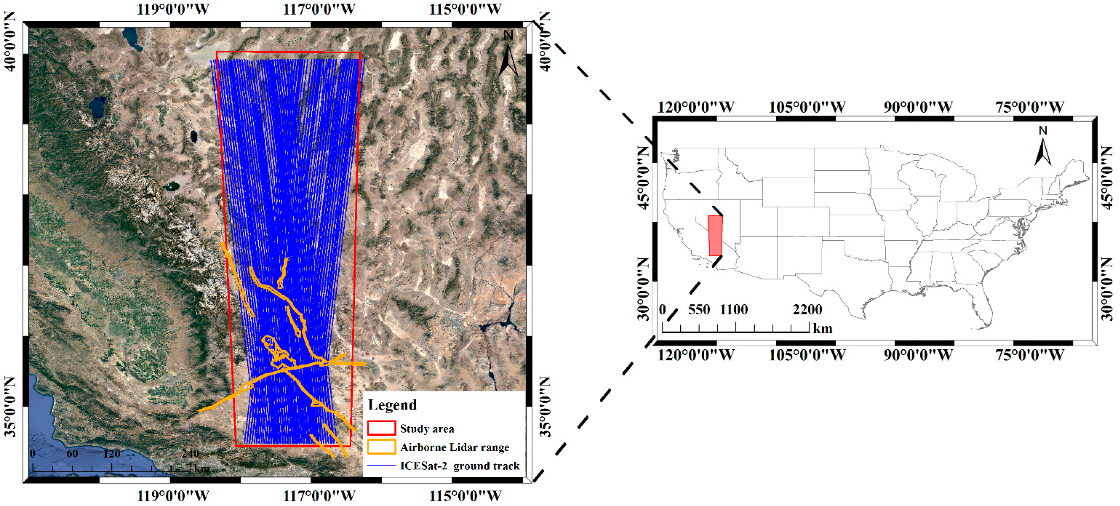
2.1.1. Study Area

The study area is located in the western United States (34.45° N–39.83° N, 116.43° W~118.40° W), on the east side of the Sierra Nevada, spanning Nevada and California, covering an area of approximately 93,294 km² (Figure 1). This study area was chosen for three reasons: (1) The topography in the south of the study area is relatively flat, with rolling hills in the north. The elevation difference of the whole area is about 4000 m, and the terrain features are rich; (2) the vegetation in the study area is sparse, the distribution of trees, crops and water is small; it is mainly composed of bare land and low shrubs or grasses, the land cover type is simple and stable, and the interannual and seasonal changes are relatively small; (3) the acquisition rate of spaceborne laser data is high, and the airborne lidar data with wider coverage and higher timeliness can be used as reference data. Therefore, this study area represents a good choice for long-term spaceborne laser data crossover analysis and calibration.

2.1.2. ICESat-2 Data

At an orbital altitude of 500 km, ICESat-2 performs measurements with a repeating period of 91 days at an orbital inclination of 92°, and its sub-satellite point track forms 1387 virtual reference ground tracks (RGT) on the Earth’s surface. The actual measurements are located on either side of the RGT, with six individual laser beams forming the measurement profile on the ground [39,40]. The six ICESat-2 beams are divided into three pairs, and the transmission energy ratio of weak and strong beams in each pair is 1:4. In this study, we downloaded and processed all laser beam data acquired by the ICESat-2 satellite in the study area from 2019 to 2021 (Figure 1), specifically including 12 repetition cycles (from C02 to C13) and 8 reference ground tracks (including RGT0082, RGT0143, RGT0440, RGT0501, RGT0585, RGT0943, RGT1027 and RGT1385). The strong and weak beam data for each RGT were used. It should be noted that due to a solar array anomaly, ICESat-2 experienced a 15-day shutdown state, resulting in no measurement data for RGT1385 for C03 and RGT0082 and RGT0143 for C04. Furthermore, as a result of influence of weather and other factors, there are no available measurement data in the study area for RGT1027 for C09, and RGT0143 and RGT0501 for C10 and C11. Ultimately, data from a total of 528 beam profiles for 88 reference ground tracks were used. The ICESat-2 data products used in this study include the ATL03 data product, with photon geolocation information (longitude, latitude, and elevation, etc.) [41], and the ATL08 data product, with photon classification labels (noise, ground, and vegetation) [42]. The association of the two data products could be extracted to photon data classified as ground [42,43]. All ICESat-2 data products are from the National Snow and Ice Data Center (https://search.earthdata.nasa.gov (accessed on 11 April 2022)), version 004.

2.1.3. Airborne Lidar Data

High-accuracy airborne lidar data were used as reference data and validation data to evaluate the absolute accuracy of ICESat-2 elevation data before and after the crossover adjustment. Considering that there were no unique airborne lidar data that can form an overlap with the ICESat-2 data for all RGTs in the study area, we downloaded two airborne lidar datasets through the open portal OpenTopography (https://portal.opentopography.org/datasets (accessed on 27 May 2022)), including Ridgecrest, CA Post-Earthquake Lidar Collection (CA19_redge3) dataset, and EarthScope Southern & Eastern California LiDAR Project (SoCAL) dataset [44]. The CA19_redge3 data were collected from 27 July to 2 August 2019, covering an area of 784.42 km² with a point density of 33.13 pts/m². The elevation accuracy of point cloud data is less than 0.05–0.1 m (1σ). SoCAL data were collected earlier (4 February 2007–4 June 2007). The coverage area and point density are 1683 km² and 4.61 pts/m², respectively. The elevation accuracy of point cloud data is less than 0.05–0.3 m (1σ). The horizontal and vertical datums of the airborne lidar data and the ICESat-2 laser data are both WGS84 ellipsoids, and the airborne lidar data were classified into ground points and non-ground points.

2.1.4. Ancillary Data

To assess the effect of the terrain slope and land cover type on the accuracy of crossover data, we introduced auxiliary data. The terrain slope was generated from 10 m resolution Digital Elevation Model (DEM) data from the study area, produced by the United States Geological Survey (USGS) (https://portal.opentopography.org/datasets (accessed on 27 May 2022)). Figure 2a shows the raster map of the terrain slope distribution in the study area calculated by the ArcGIS software. The terrain slope of the study area is large, ranging from 0 to 82°. The topography in the south is extremely flat, and the central and northern areas are dominated by mountains.

The land cover type information comes from the 2020 10 m resolution global land cover dataset (https://www.arcgis.com/apps/instant/media (accessed on 21 April 2022)) provided by the Environmental Systems Research Institute (ESRI). The dataset was generated by a deep learning model and is one of the land cover datasets with the highest spatial resolution so far. As shown in Figure 2b, the land cover types were divided into 11 categories: water, trees, grass, flooded vegetation, crops, shrub, built area, bare land, snow/ice, clouds, and rangeland (natural meadows and fields with sparse to no tree cover, open savanna with few to no trees, parks/golf courses/lawns, pastures.), with an overall accuracy rate of 86% [45]. The land cover in the study area is dominated by rangeland and bare land, with a small amount of water, trees and built areas, which are sparsely distributed. Given that the spatial resolution of the terrain slope and land cover type dataset was sufficient, we directly extracted the terrain slope and land cover type information corresponding to each crossover location.

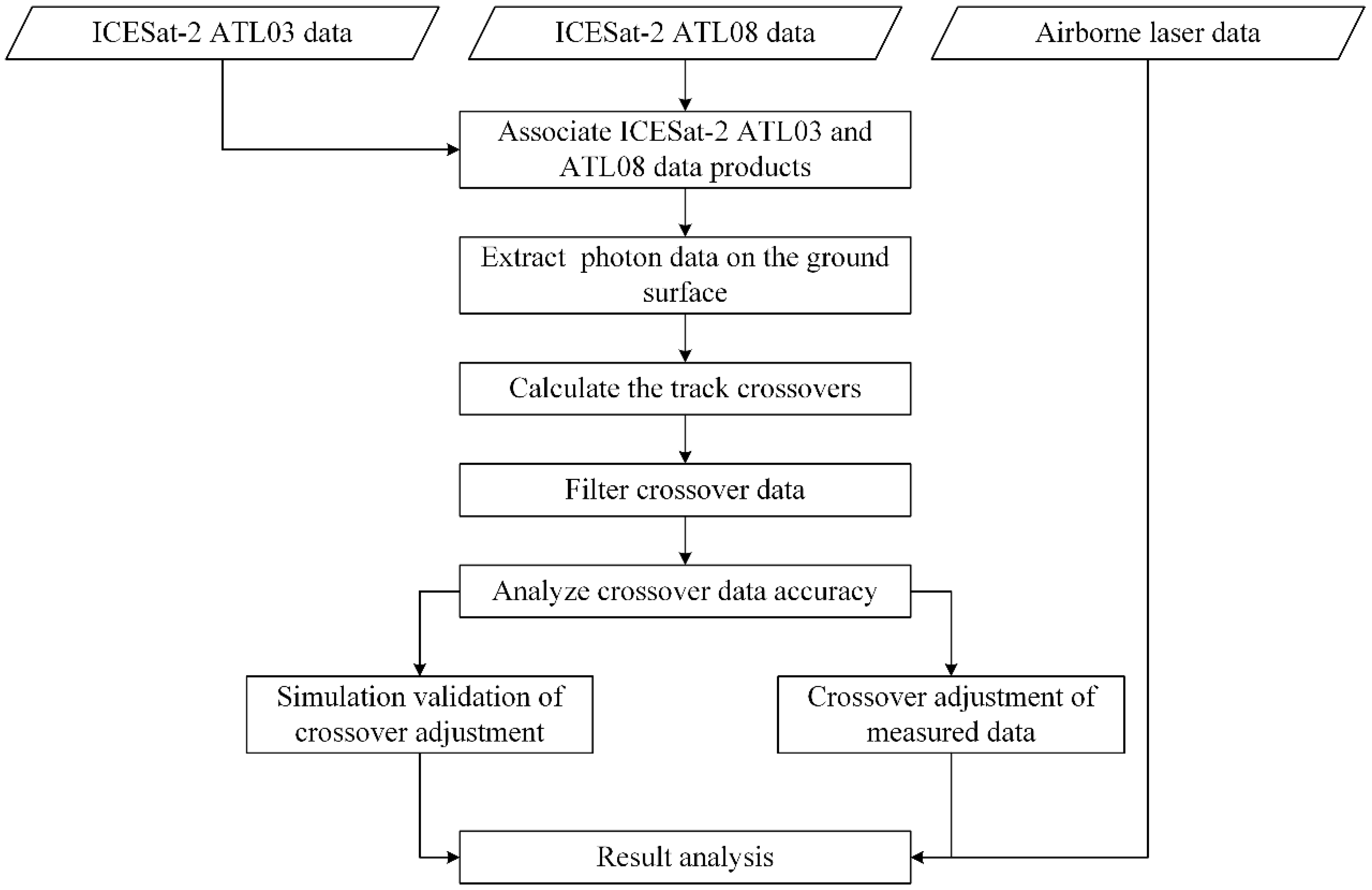
2.2. Crossover and Crossover Adjustment

The crossover calculation is the basis of the crossover adjustment. Given the higher sampling frequency and increased number of laser beams of ICESat-2/ATLAS, the point cloud spacing is extremely small. Moreover, in the low and middle latitudes, ICESat-2 is not strictly aligned with the RGT to achieve accurate repeated measurements [40], and the periodicity of the orbit cannot be used to calculate the position of the crossover. Crossovers must be calculated beam by beam [46]. Here, we designed a method flow for calculating the crossovers of ICESat-2 laser data. The basic principle is that the laser point with the closest distance in the two laser beams is the crossover. The steps are as follows:

• Determine whether there is a crossover between any two beams. According to the following conditions: (a) the minimum longitude of the ascending arc should be less than the maximum longitude of the descending arc; (b) the maximum longitude of the ascending arc should be greater than the minimum longitude of the descending arc. Thus, we can preliminarily determine whether there is a crossover between any two beams.
• Locate the area where the crossover exists. Calculate the latitude difference corresponding to the laser point at the same longitude position of the two beams. The location where the difference changes from positive to negative or from negative to positive is the area where the crossover exists, and the potential crossover is located among the four laser points (two laser points per beam) in the area.
• Obtain the crossover. Calculate the distance between any two laser points between different beams, and the two points with the smallest distance (must be less than 0.7 m) are the final crossover.

As shown in Figure 3, on the basis of 528 beam profiles of 88 reference ground track acquired by ICESat-2/ATLAS in the study area, we obtained a total of 21,439 crossovers for the entire period. The color map shows the magnitude of the crossover differences. It can be found that there are very few crossovers with differences greater than 10 m.

Table 1. The range of crossover differences.

Crossover Differences (m)	0–5	5–10	10–15	15–20	>20
Number	21,292	103	31	8	5
STD (m)	0.66	6.78	12.43	18.56	31.17
Percentage (%)	99.31%	0.48%	0.15%	0.04%	0.02%

shows the distribution range of the crossover differences. Only 0.21% of the crossovers have differences greater than 10 m, and the number of crossovers with differences less than 10 m accounts for 99.79%. The crossover difference is affected by a combination of factors. In order to avoid the excessive crossover difference affecting the subsequent adjustment processing, we only used the crossovers with stable land cover types (bare land, built area, and rangeland) and differences of less than 10 m. Therefore, 21,315 crossovers were effective.

Crossover analysis provides an important method for evaluating data quality, since over a solid surface, neglecting tides and seasonal surface changes, the altitude of the ground spot is constant [12]. At the crossover location, for the ascending and descending arc segment, the following was established:

$$\widehat{H}=H_{obs}^a+f^a,$$

(1)

$$\widehat{H}=H_{obs}^d+f^d,$$

(2)

where a and d represent the ascending arc segment and descending arc segment, respectively; $\widehat{H}$ and $H_{obs}$ are the adjusted and observed values of ground elevation, respectively; and $f$ is the error model. For the adjustment of regional crossovers, the corresponding error model was provided in theoretical research [47]. Considering that the experimental area is small, the error of each beam should be relatively stable in the local region, and the constant model is selected as the final adjustment model, i.e., $f=\mathsf{\delta }$. The $\mathsf{\delta }$ is a composite of the ranging precision of the instrument, the radial orbital uncertainty, the geolocation knowledge, forward scattering in the atmosphere, and tropospheric path delay uncertainty. The crossover difference is the comprehensive reflection of various uncertainties in the altimetry data.

According to the constraint condition that the elevations at the crossovers are the same, for the i-th ascending arc segment and the j-th descending arc segment, the following observation equation can be established:

$$l_{ij}=-f_i^a+f_j^d-\left(H_{obs,i}^a-H_{obs,j}^d\right)=-{\delta }_i^a+{\delta }_j^d-\left(H_{obs,i}^a-H_{obs,j}^d\right),$$

(3)

where $H_{obs,i}^a-H_{obs,j}^d=d{h}_{i,j}$ is the crossover difference (i = 1, 2, …, q; j = 1, 2, …, s). For multiple ascending arc segments and multiple descending arc segments in the study area, the following error equation in matrix form can be formed:

$$V=A\widehat{X}-L,$$

(4)

where A is the coefficient matrix, L is the observed value vector, and $\widehat{X}$ is the unknown parameter vector, as follows:

$$A=\left[\begin{array}{cc}\mathit{q}& \mathit{s}\\ ⏞& ⏞\\ \begin{array}{cccc}-1& & & \\ -1& & & \\ ⋮& & & \\ -1& & & \\ & -1& & \\ & -1& & \\ & ⋮& & \\ & -1& & \\ & & \ddots & \\ & & & -1\\ & & & -1\\ & & & ⋮\\ & & & -1\end{array}& \begin{array}{cccc}1& & & \\ & 1& & \\ & & \ddots & \\ & & & 1\\ 1& & & \\ & 1& & \\ & & \ddots & \\ & & & 1\\ & ⋮& & \\ 1& & & \\ & 1& & \\ & & \ddots & \\ & & & 1\end{array}\end{array}\right],$$

(5)

$$\widehat{X}={\left[{\delta }_1^a, {\delta }_2^a, \cdots ,{\delta }_q^a, {\delta }_1^d, {\delta }_2^d, \cdots ,{\delta }_s^d\right]}^T,$$

(6)

$$\begin{gathered} L={\left[H_{obs,1}^a-H_{obs,1}^d, H_{obs,1}^a-H_{obs,2}^d, \cdots , H_{obs,1}^a-H_{obs,s}^d, H_{obs,2}^a-H_{obs,1}^d, H_{obs,2}^a \\ -H_{obs,2}^d, \cdots , H_{obs,2}^a-H_{obs,s}^d, \cdots ;H_{obs,q}^a-H_{obs,1}^d, H_{obs,q}^a \\ -H_{obs,2}^d, \cdots , H_{obs,q}^a-H_{obs,s}^d\right]}^T, \end{gathered}$$

(7)

The parameter $\mathsf{\delta }$ of each arc segment can is obtained by the least square method:

$$\widehat{X}={\left(A^{T}PA\right)}^{-1}{A}^{T}PL,$$

(8)

and then the adjusted elevation can be calculated as:

$$\widehat{H}=H_{obs}+ \overrightarrow{\mathsf{\delta }}.$$

(9)

The workflow for laser data quality analysis and calibration based on crossovers is shown in Figure 4. First, the terrain points were extracted by associating the ICESat-2 ATL03 and ATL08 data products; then, the crossovers of all beams were calculated beam by beam. Next, data at crossovers located in water, trees, and crop types and with differences of greater than 10 m were filtered out (this threshold was obtained from our experimental analysis). Thereafter, the spatiotemporal characteristics and accuracy performance of the remaining crossover data were analyzed. Finally, crossover adjustment experiment was carried out, which was divided into the simulation validation of crossover adjustment and crossover adjustment based on ICESat-2 measured data. Furthermore, the airborne lidar terrain data were used to validate the data accuracy before and after adjustment.

2.3. Accuracy Validation

The crossover difference between ascending and descending arcs and the difference between the spaceborne data and the airborne data were calculated as follows:

$$d{h}_{crossover}=H_{spaceborne}^a-H_{spaceborne}^d,$$

(10)

$$d{h}_{space/air}=H_{spaceborne}-H_{airborne},$$

(11)

Several statistical indicators were calculated based on dh values, including standard deviation (STD), bias, mean absolute error (MAE), maximum (MAX), minimum (MIN), root mean square error (RMSE), and coefficient of determination (R²).

$$STD=\frac{1}{n}{{\displaystyle \sum }}_{i=1}^n\left(dh-\overline{dh}\right),$$

(12)

$$Bias=\frac{1}{n}{{\displaystyle \sum }}_{i=1}^n\left(dh\right),$$

(13)

$$MAE=\frac{1}{n}{{\displaystyle \sum }}_{i=1}^n\left|dh\right|,$$

(14)

$$RMSE=\sqrt{\frac{1}{n}{{\displaystyle \sum }}_{i=1}^n\left(dh\right)}.$$

(15)

3. Results

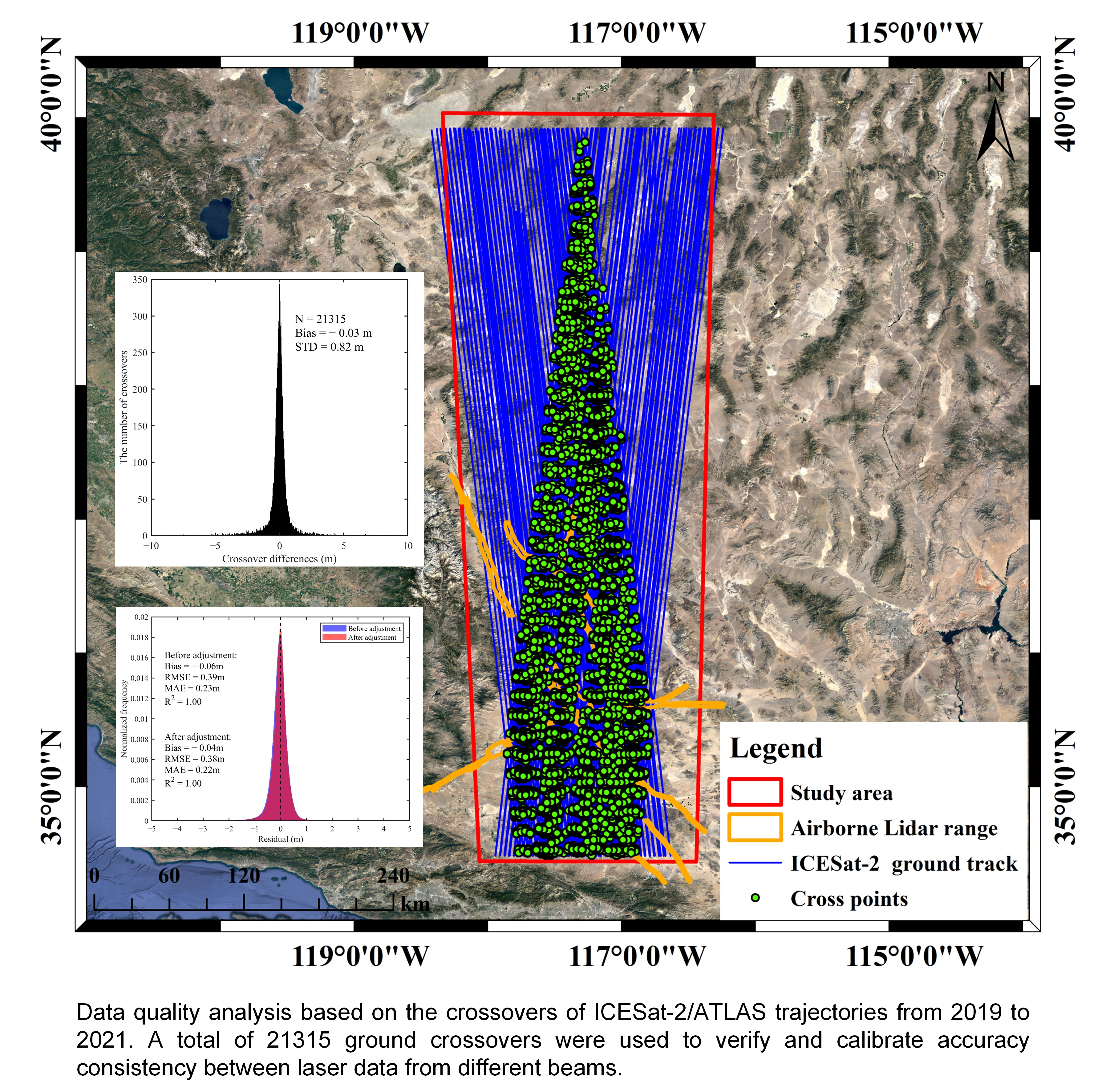
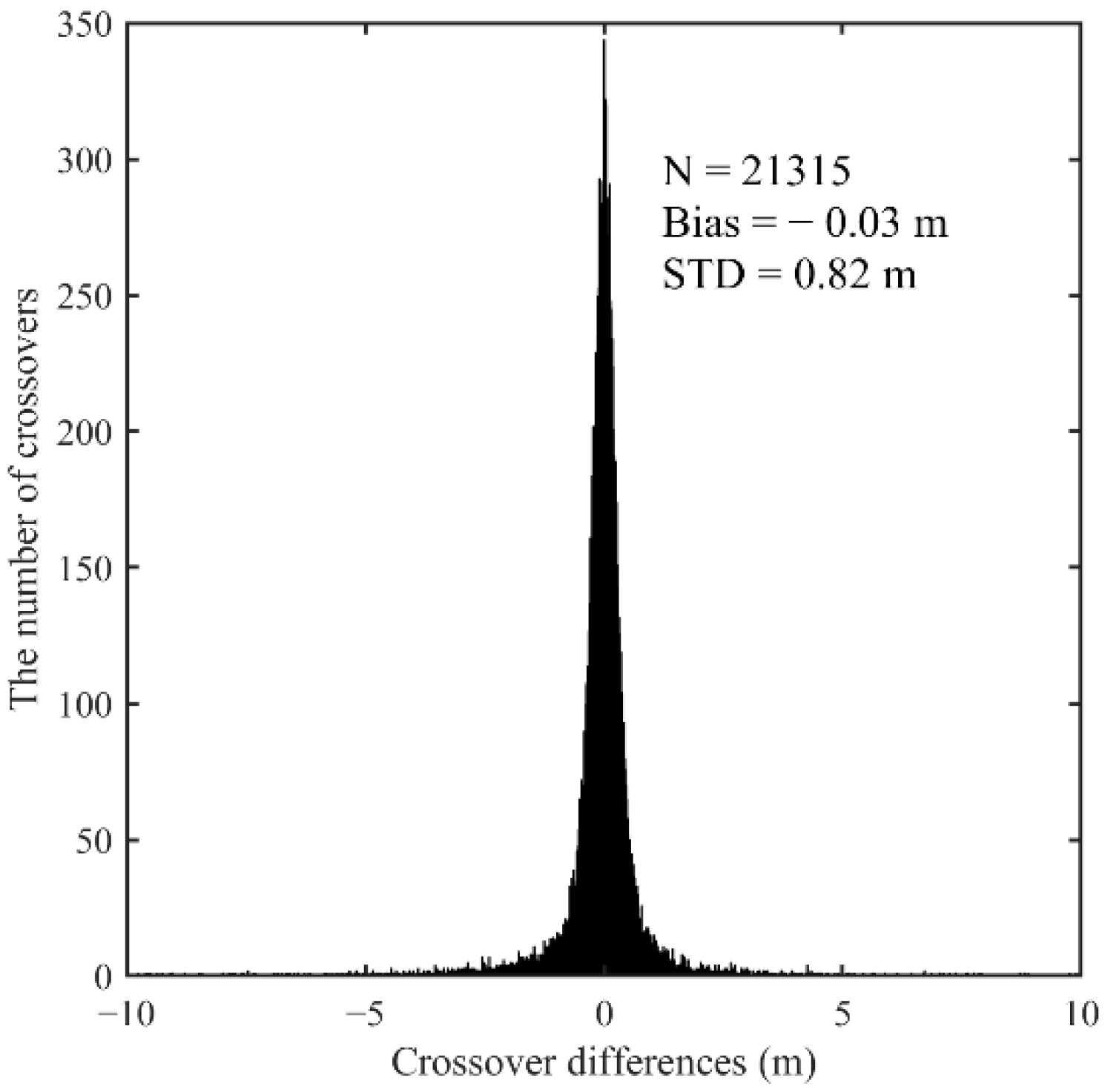
3.1. Crossovers Accuracy Analysis

As shown in Figure 5, the high agreement between the different beams of ICESat-2 is shown by the peak distribution of residual values around zero. The STD and bias of the 21,315 valid crossovers in the study area were 0.82 m and −0.03 m, respectively.

Analyzing the time-varying rule of the crossover difference of each beam is a key step in the adjustment [26,29]. Figure 6 shows the variation of the crossover differences with observation time. It was found that, regardless of whether it was relative to the absolute observation time or the time span, the distribution of the crossover differences was relatively stable, and there was no significant systematic bias on the whole or locally. Figure 7 shows the distribution of crossover differences for each RGT. Blank areas are caused by missing data. The crossover differences of any track (including the six beams) were relatively symmetrically distributed around the 0 value, indicating that the data products of ICESat-2 have a high relative measurement accuracy. It should be noted that main systematic biases in the ICESat-2 data products were calibrated [16,47,48]. However, ATL03 data products may still have small residual systematic biases [22,41].

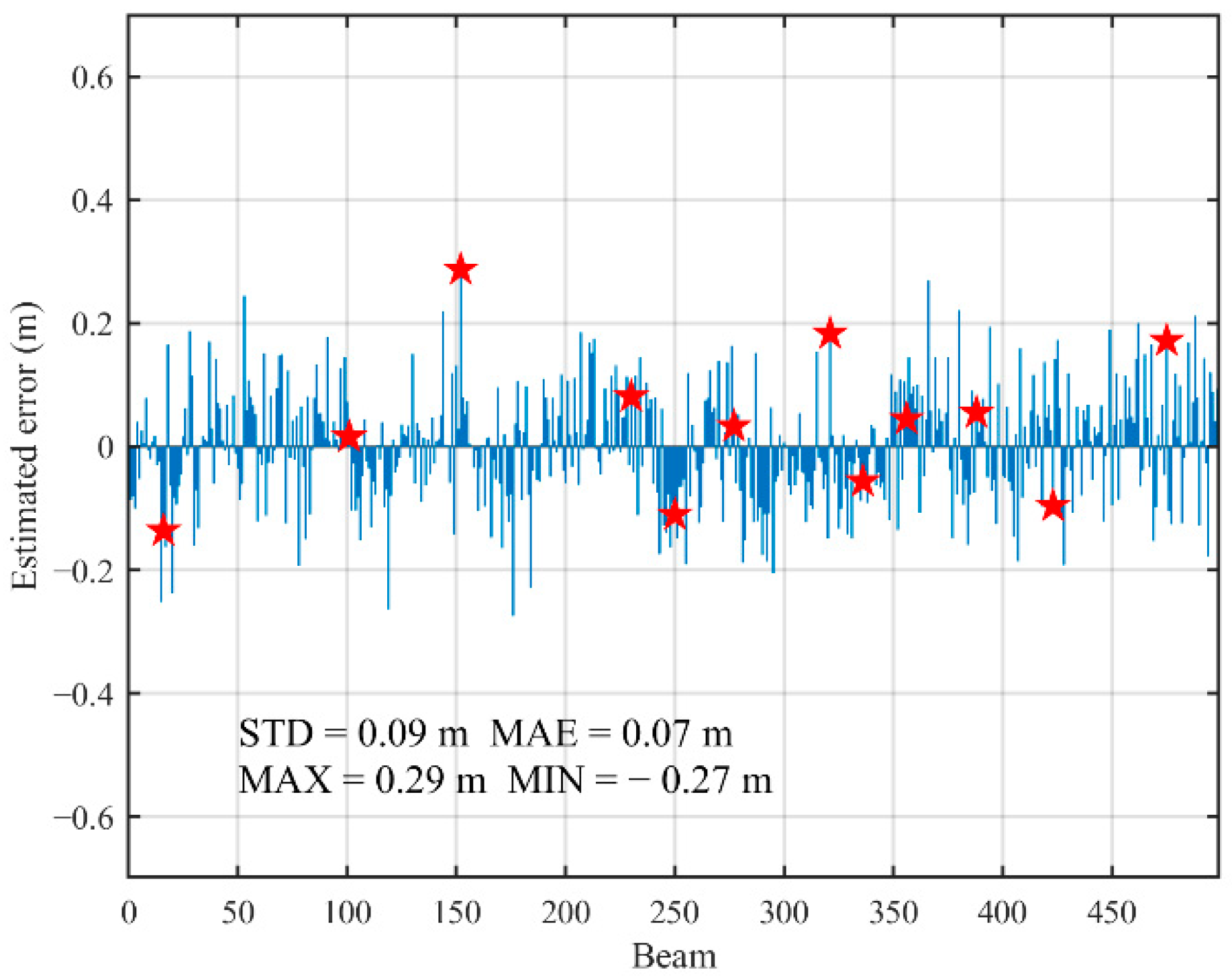
3.2. Simulation Validation of Crossover Adjustment

Considering that the systematic bias in the ICESat-2 data product had calibrated, we randomly added a systematic bias in the range of [−0.5 m, 0.5 m] to the elevation data of some beams to obtain trajectory data with biases, so as to validate the effectiveness of the adjustment method. Note that the bias of 0.5 m refers to the conclusion of the simulation study of the ICESat-2/ATLAS official algorithm group. When the laser off-pointing is 5°, the radial error will reach 0.43 m (the 5° represents the off-pointing limit for science collection, and generally off-pointing will not exceed 1.7°) [49]. The beams with added biases are distributed at different RGTs and periods; see

Table 2. ICESat-2 data with added systematic biases.

Date	RGT	Cycle	Strong/Weak	Beam
20190130	0501	02	strong	gt1l
20190604	1027	03	strong	gt1l
20190730	0501	04	strong	gt1l
20191002	0082	05	strong	gt2r
20200203	0585	06	strong	gt1r
20200428	0501	07	weak	gt1l
20200826	0943	08	strong	gt2l
20201223	1385	09	strong	gt3l
20200223	0943	10	weak	gt3l
20210422	0440	11	strong	gt1r
20210922	1385	12	strong	gt3r
20211001	0143	13	weak	gt3l

for details.

Table 3. Residuals of crossover differences before and after adjustment.

	STD (m)	Bias (m)	MAX (m)	MIN (m)
Before adjustment	0.82	−0.02	9.91	−9.78
After adjustment	0.80	0.00	9.47	−9.83

lists the residual results of the crossover difference before and after adjustment. The adjustment reduced the residual at the crossover, and the STD was reduced from 0.82 m to 0.80 m. The estimated systematic bias of each beam after adjustment is shown in Figure 8. The red star represents the beam with the added bias. It was found that, excepting for the beams marked with a star, the estimated systematic biases of almost all beams were distributed within ±0.20 m, and most of the estimated systematic biases were less than 0.10 m. The STD of the estimated systematic bias of all beams was 0.10 m, and the MAE was 0.08 m.

In order to explore the accuracy change in the data from each beam before and after adjustment, Figure 9 shows the adjustment results of the data from the 12 laser beams marked by the red star, i.e., the laser data with added errors. Each beam is plotted as along-track distance and elevation. The blue and red scatter points represent the spaceborne laser data before and after adjustment, respectively, and the green scatter points are the airborne lidar data. Furthermore, a local enlarged image at the position of the black dashed box is provided to better show the adjustment results. Although the spaceborne laser data exhibited greater spread (roughness) than the airborne lidar data, for all 12 beams, the spaceborne laser data fitted the airborne lidar data better after adjustment than before adjustment. For beams 0501-02-strong-gt1l, 1027-03-strong-gt1l, 0501-04-strong-gt1l, 0585-06-strong-gt1r, 1385-09-strong-gt3l, 0943-10-weak-gt3l and 0143-13-weak-gt3l, the adjusted spaceborne laser data are in better agreement with the airborne lidar data. For beams 0082-05-strong-gt2r, 0501-07-weak-gt1l, 0943-08-strong-gt2l and 1385-12-strong-gt3r, the changes in spaceborne laser data before and after the adjustment are all small, and are always in agreement with the airborne lidar data.

Table 4. Comparison of data accuracy for simulation validation of crossover adjustment.

Beam	Number	Added Error (m)	Estimated Error (m)	Difference (m)	Before Adjustment	After Adjustment
					RMSE (m)
0501-02-strong-gt1l	13,320	−0.41	0.30	−0.11	0.43	0.23
1027-03-strong-gt1l	6140	0.34	−0.33	0.01	0.47	0.34
0501-04-strong-gt1l	12,862	−0.19	0.22	0.03	0.30	0.15
0082-05-strong-gt2r	10,144	−0.12	−0.02	−0.14	0.20	0.20
0585-06-strong-gt1r	9939	−0.32	0.40	0.08	0.31	0.26
0501-07-weak-gt1l	17,254	0.19	−0.01	0.18	0.25	0.25
0943-08-strong-gt2l	10,811	−0.11	0.05	−0.06	0.35	0.33
1385-09-strong-gt3l	10,159	0.36	−0.32	0.04	0.41	0.24
0943-10-weak-gt3l	22,065	0.44	−0.27	0.17	0.72	0.66
0440-11-strong-gt1r	6675	0.22	−0.31	−0.09	0.54	0.58
1385-12-strong-gt3r	23,960	−0.12	0.17	0.05	0.30	0.23
0143-13-weak-gt3l	15,757	−0.22	0.51	0.29	0.50	0.31

details the number of laser points for the 12 beams, the added system bias, the estimation of the system bias, and the accuracy of the spaceborne laser data before and after adjustment. Overall, the magnitude of the bias estimate can better reflect the added bias, with an MAE of 0.10 m. For beams 1027-03-strong-gt1l, 0501-04-strong-gt1l, 0585-06-strong-gt1r, 0943-08-strong-gt2l, 1385-09-strong-gt3l, 0440-11-strong-gt1r, and 1385-12-strong-gt3r, the difference between the bias estimate and the added bias was less than 0.09 m. For beams 0501-02-strong-gt1l, 0082-05-strong-gt2r, 0501-07-weak-gt1l, 0943-10-weak-gt3l, and 0143-13-weak-gt3l, the difference between the bias estimate and the added bias was greater than 0.11 m. Preliminary analysis suggests that these beams may contain relatively large systematic biases, and the bias estimate after adjustment was a comprehensive reflection of the added bias and the original bias. Section 3.3 provides an estimate of the original systematic bias for each beam. Excepting beam 0440-11-strong-gt1r, the RMSE of the elevation data for the other beams decreased after adjustment, with an average decrease of 23.38%. In conclusion, the experimental results of the simulation validation well demonstrate that the crossover adjustment can calibrate potential systematic biases in elevation data and improve the internal consistency among all beam data.

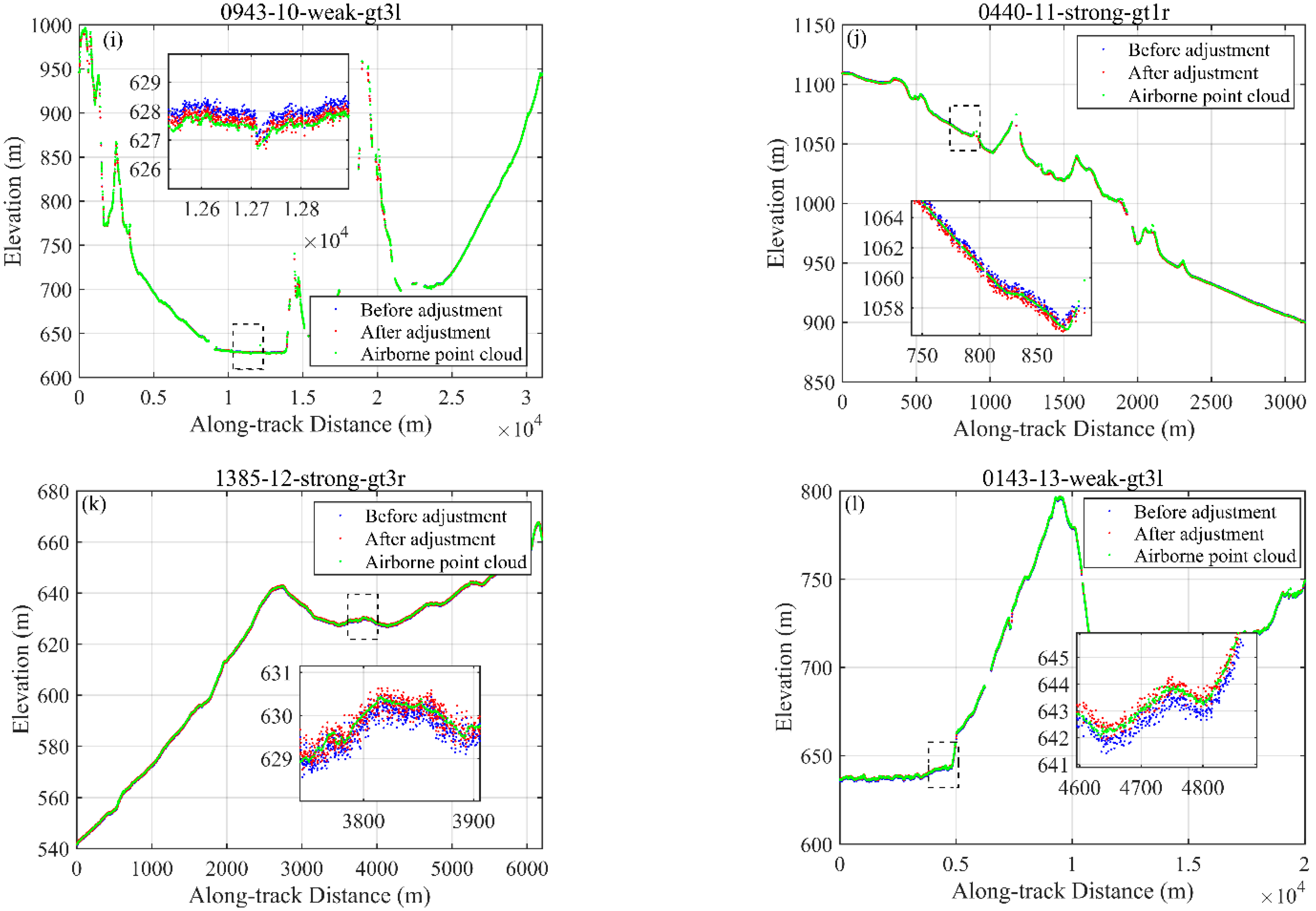
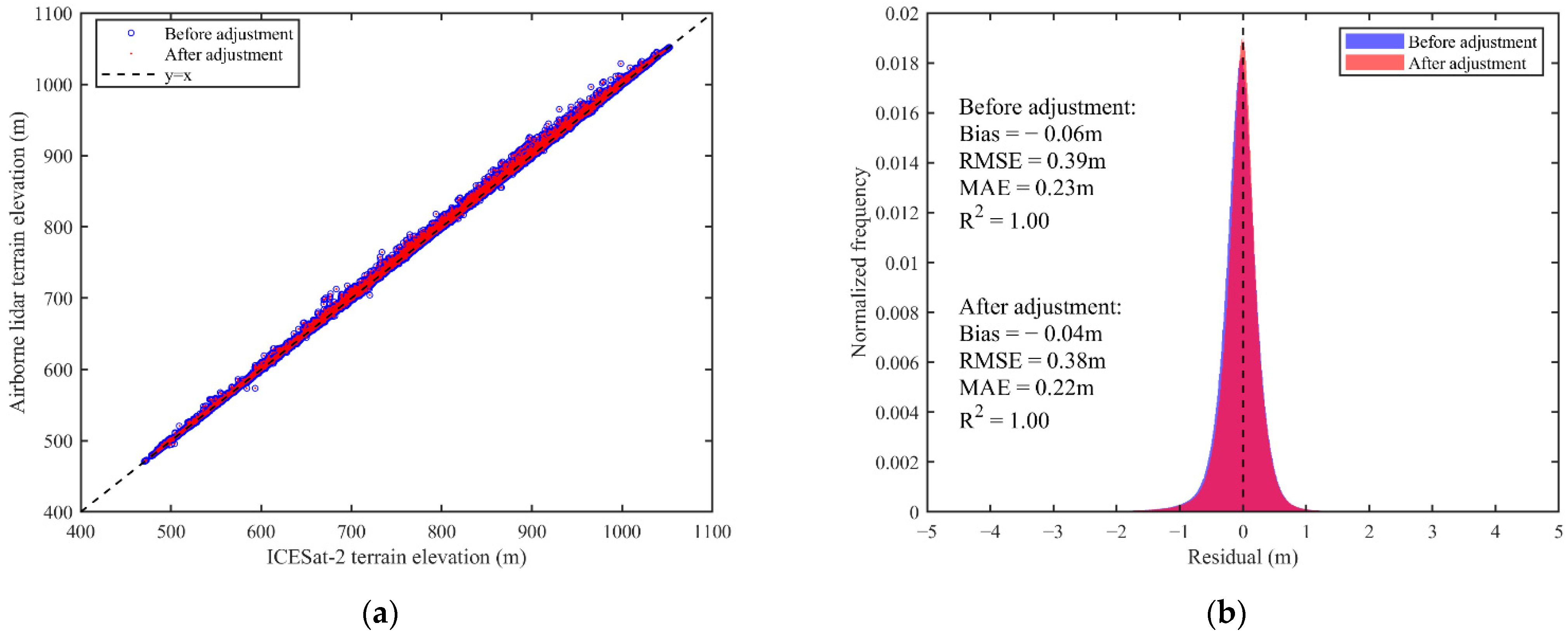
3.3. Validation and Analysis of ICESat-2 Measured Data

Although we did not find a significant systematic bias in the ICESat-2 terrain data in our previous analysis, we still conducted crossover adjustment experiments and, herein, provide the corresponding results. After adjustment, the STD of the crossover differences decreases from 0.81 m to 0.80 m. The improvement of only 0.01 m indicates that the bias of ICESat-2 terrain data between different beams was very small. As shown in Figure 10, the STD of the estimated systematic bias for all beams was 0.09 m and the MAE was 0.07 m. This is nearly consistent with the conclusion of a previous study [22], which showed that the ICESat-2 data product had a ranging bias of 0.13 m. The maximum and minimum systematic bias estimates were 0.29 and −0.27 m, respectively.

Table 5. Comparison of data accuracy before and after crossover adjustment based on ICESat-2 measured data.

Beam	Number	Estimated Error (m)	Before Adjustment	After Adjustment
			RMSE (m)
0501-02-strong-gt1l	13,320	−0.11	0.21	0.22
1027-03-strong-gt1l	6140	0.02	0.34	0.34
0501-04-strong-gt1l	12,862	0.03	0.16	0.14
0082-05-strong-gt2r	10,144	−0.14	0.22	0.20
0585-06-strong-gt1r	9939	0.08	0.21	0.25
0501-07-weak-gt1l	17,254	0.18	0.30	0.26
0943-08-strong-gt2l	10,811	−0.06	0.32	0.33
1385-09-strong-gt3l	10,159	0.04	0.25	0.24
0943-10-weak-gt3l	22,065	0.17	0.68	0.66
0440-11-strong-gt1r	6675	−0.10	0.56	0.59
1385-12-strong-gt3r	23,960	0.06	0.25	0.23
0143-13-weak-gt3l	15,757	0.29	0.35	0.31

details the results before and after adjustment for the beams marked by the red star in Figure 10. It was found that, for beams 0501-02-strong-gt1l, 0082-05-strong-gt2r, 0501-07-weak-gt1l, 0943-10-weak-gt3l and 0143-13-weak-gt3l, the systematic bias estimate was larger. This is the reason for the large difference between the estimated systematic bias and the added bias for these beams in the previous section. The systematic bias estimate for seven beams (1027-03-strong-gt1l, 0501-04-strong-gt1l, 0585-06-strong-gt1r, 0943-08-strong-gt2l, 1385-09-strong-gt3l, 0440-11-strong-gt1r and 1385-12-strong-gt3r) was less than 0.10 m. As compared with the case before adjustment, the change in RMSE after adjustment was limited. The RMSE after adjustment for some beams was increased by several centimeters. As compared to ICESat-2’s nominal terrain measurement accuracy of 0.10 m, its fluctuation can be considered to be small. It should be noted that we did not expect that the absolute accuracy of the terrain data of all beams to be improved after adjustment; because the crossover adjustment did not rely on external data sources, it only used the system’s own measurement data to improve the internal accuracy between long-term data.

We also calculated the absolute accuracy of the elevations of all the spaceborne laser data in the area covered by the airborne data of CA19_redge3 before and after adjustment. All beam data were not evaluated because we believe that the SoCAL airborne data is relatively old (acquired in 2007) and cannot guarantee the stability of terrestrial features within its coverage. Finally, a total of 7,093,102 terrain data points were extracted. Both before and after adjustment, the very high R² value indicates that the terrain elevations retrieved by ICESat-2 well matched the airborne lidar terrain elevations (Figure 11a). Similarly, the residual results before and after the adjustment (Figure 11b) show that the distribution of the ICESat-2 and the airborne lidar terrain elevations were also nearly consistent, i.e., very close to the real terrain height. As compared with the RMSE of the ICESat-2 terrain elevation of 0.39 m before adjustment, the improvement in terrain elevation accuracy after adjustment was limited (RMSE = 0.38 m). The accuracy evaluation results of the terrain elevation in this paper are in agreement with the RMSE result of 0.38 m by Liu et al. [50], and better than the terrain elevation RMSE of 0.75 m and 0.73 m from the previous studies of Xing et al. [43] and Neuenschwander et al. [51]. The main reason for this is that the land cover of the study area in this paper was almost bare land or was only covered with sparse vegetation, which was similar to the conditions in the study area (tundra) of Liu et al. [24]. The study areas of Xing et al. [43] and Neuenschwander et al. [51] were covered with dense vegetation. The bias of −0.06 m before adjustment indicates that the terrain elevation of ICESat-2 slightly underestimated the true terrain height, which is almost consistent with the conclusion of the Liu et al. [50] study (bias = −0.07 m). The bias between the ICESat-2 elevation and the airborne terrain elevation after adjustment was slightly improved (bias = −0.04 m), which confirms the effectiveness of the study method in this paper.

4. Discussion

4.1. Influencing Factors of Crossover Differences

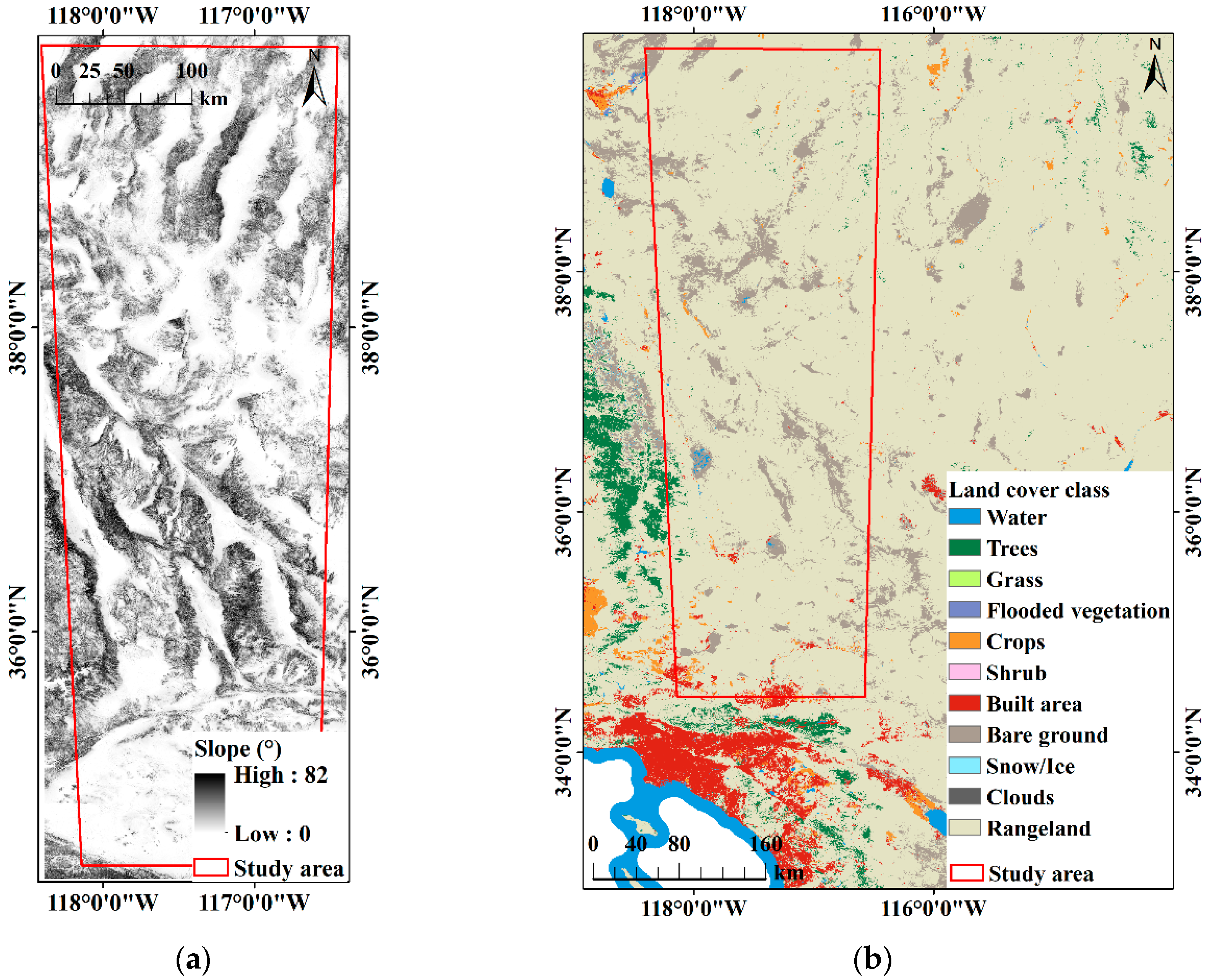
4.1.1. Effect of Terrain Slope on Crossover Differences

Table 6. Accuracy statistics of crossover difference in different terrain slopes.

	Terrain Slope (°)	0–5	5–10	10–15	15–20	20–25	25–30	>30
All crossovers	Number	11,035	2937	2319	2020	1447	909	772
	STD (m)	1.16	1.14	0.90	1.08	0.82	0.95	0.93
Crossovers (difference < 10 m)	Number	11,009	2930	2316	2015	1446	908	771
	STD (m)	0.82	0.86	0.78	0.80	0.76	0.86	0.80

shows the accuracy of crossover difference in different terrain slopes. The number of crossovers decreased significantly with increase in slope, which was jointly determined by the topographic characteristics of the study area and the trajectory distribution characteristics of ICESat-2. It was found that there was no significant correlation between the accuracy of crossovers and terrain slope, especially when the crossover difference value was less than 10 m. We also listed the accuracy performance of ICESat-2 data before and after adjustment in different slopes (

Table 7. Accuracy of the ICESat-2 data before and after adjustment in different terrain slopes.

	Terrain Slope (°)	0–5	5–10	10–15	15–20	20–25	25–30	>30
	Number	6,158,823	655,499	165,507	60,282	30,516	14,155	8320
Before adjustment	Bias (m)	−0.04	−0.09	−0.20	−0.45	−0.70	−1.04	−1.38
	RMSE (m)	0.28	0.50	0.83	1.27	1.69	2.26	2.69
After adjustment	Bias (m)	−0.02	−0.08	−0.19	−0.43	−0.68	−1.02	−1.36
	RMSE (m)	0.27	0.50	0.82	1.27	1.69	2.25	2.68

). It was found that the accuracy of ICESat-2 data decreases gradually with the increase in slope. This may be caused by geolocation errors present in the ICESat-2 data. The accuracy of the adjusted ICESat-2 terrain data was improved but not significantly. The possible reason is that the elevation error caused by the small geolocation error (the geolocation accuracy after the maneuvering scan calibration is 3.2 m at the ocean surface; the geolocation accuracy calculated by CCR on the ground is 3.7 m) [16,35] is difficult to be reflected by the crossover difference.

4.1.2. Effect of Land Cover Types on Crossover Differences

As a statistical index to evaluate the relative accuracy of laser altimetry data, it is very important to reduce the error caused by external time-varying factors.

Table 8. Accuracy statistics of crossover difference in different land cover types.

	Land Types	Water	Trees	Crops	Built Area	Bare Land	Rangeland
All crossovers	Number	1	17	62	144	2082	19,133
	STD (m)	-	0.60	0.56	1.26	1.11	1.09
Crossovers (difference < 10 m)	Number	1	17	62	143	2074	19,098
	STD (m)	-	0.60	0.56	0.85	0.82	0.82

shows the number and accuracy of the crossover in different land cover types in the study area. A larger number of crossovers were located in relatively stable and simple land cover types, such as rangeland, bare land, and built area. The number of crossovers located in relatively complex water, tree and crop types was low. This distribution of crossovers in the study area helped us to analyze the relative accuracy of ICESat-2 data. The STD of the crossover data located in tree and crop type was smaller, i.e., 0.60 m and 0.56 m, respectively. The STD of the data was larger in the built area, bare land, and rangeland types. This phenomenon may be caused by large differences in the number of crossovers in different land cover types and abnormal crossovers in built, bare land, and rangeland types. With a 10 m crossover difference filter threshold, the STD in built, bare land, and rangeland dropped significantly, and the number of points did not change significantly. This shows that there are indeed abnormal points in these land types. The number of abnormal crossovers is very small, and the distribution in space is random. Land cover types such as water, trees and crops are usually time-varying. The relatively small STDs in this study can be considered as special cases, and in order to be consistent with future studies, we excluded them from the analysis.

4.2. Adjustment Model Analysis

The radial orbit error is the main error source in traditional crossover adjustment. With the improvement of satellite orbit determination technology, the orbit error in altimeter data is well controlled [52]. On-orbit calibration and validation show that the ICESat-2 precise orbit determination (POD) system achieves a radial orbit accuracy of 1.5 cm, more than twice the mission orbit accuracy requirement of 3.0 cm [48]. The magnitude of its impact is already comparable to other error sources such as ranging, geolocation, atmospheric scattering, and tropospheric delays. Therefore, the laser altimeter data are affected by various dynamic system errors, and the comprehensive effect of these errors is more complex. It is a crude but effective method to simplify the various influencing factors to a constant error in the experiment. First, the adjustment experiment takes the beam as the basic unit. All laser spots in each beam are considered to have similar systematic biases (if any) within the study area, while the biases between different beams are considered to be different. The potential systematic bias of each beam is estimated by minimizing the differences of a large number of crossovers (the mean number of crossovers per beam is about 80) between beams using the least-squares method. This systematic bias estimate is the combined result of various errors during data collection. Second, ICESat-2/ATLAS has a very high sampling density of along-track data, and crossover differences are calculated from actual measurements (the average inter-pair distance of 21,315 valid crossovers is 0.28 m). This avoids the problem in previous studies of small biases in altimeter data being difficult to detect due to large interpolation errors. Finally, the results of comparison with CA19_redge3 airborne data show that the data accuracy of most spaceborne beams remains stable or increases after adjustment (75%), while the accuracy of few beams decreases (25%). The decrease is limited, with mean and median values of 3 cm and 2 cm, respectively. Therefore, the preliminary results from this study show that crossover adjustment can be used to validate and calibrate the accuracy of ICESat-2/ATLAS laser data, and that the constant model is simple but effective.

4.3. Innovations, Applications, and Limitations

On the basis of the large number of trajectory crossovers in ICESat-2, we were the first attempt to analyze the accuracy consistency between long-term terrain data. A crossover adjustment method is proposed to estimate potential systematic biases of spaceborne laser data and attempt to correct for them. The experimental results show that the proposed method can evaluate and calibrate the relative bias between different beam data without losing the absolute accuracy of measurement data. In addition, we quantitatively investigated the effect of the terrain slope and land cover type on the accuracy of crossover data. While the primary goal of our study was to evaluate and calibrate the accuracy of ATL03 terrain data using crossovers, these analyses were, to some extent, an indirect examination of the sampling performance of the ICESat-2 mission and the ATL08 noise and signal photon classification algorithms. The excellent along-track data sampling density of ICESat-2 was reflected in the smaller mean distance of crossover pairs. The good accuracy performance of crossovers validated the effectiveness and reliability of the ICESat-2 ground signal extraction algorithm.

With the continuous on-orbit observation of ICESat-2 and the subsequent launch of photon-counting laser altimeter satellites with more beams, the measurement data acquired by this advanced technology will not only be used for the acquisition of high-accuracy control points worldwide, but they will also be applied in global topographic mapping and high-accuracy DEM production. Crossover analysis and adjustment are expected to effectively improve the overall consistency of data accuracy, thereby providing better data products with an excellent performance to various research communities.

However, there are some limitations in this study. First, the study did not involve the calibration of the geolocation (horizontal) bias of the laser points, and it should be noted that the geolocation bias can lead to elevation errors. Future research will further explore the potential relationship between the laser point geolocation bias and the distribution of crossover differences. The laser altimetry with its small footprint will not average out the short-wavelength effects that come from rough or vegetated topography. This may have introduced errors into our analysis. Nevertheless, there is every reason to believe that most crossovers over bare land or sparsely vegetated regions of the earth will be useful.

5. Conclusions

In this study, we explore a method for data bias analysis and calibration of spaceborne photon-counting laser altimeter based on track crossovers for the first time. First, on the basis of a large number of crossovers calculated by ICESat-2 from multiple-beam data in the study area from 2019 to 2021, the accuracy performance and spatiotemporal distribution characteristics of the crossover differences were analyzed. Then, the potential of the crossover adjustment method in evaluating the relative measurement accuracy of multi-beam data was demonstrated by simulation validation and ICESat-2 measured data. The absolute accuracy of ICESat-2 terrain data before and after adjustment was evaluated using the corresponding high-accuracy airborne lidar data. Finally, we investigated the effect of the terrain slope and land cover type on crossover differences. On the basis of the experimental results, we drew the following conclusions: (1) The STD and bias of the crossovers formed by ICESat-2 terrain data were 0.82 m and −0.03 m, respectively; (2) simulation experiment verifies the effectiveness of this research method, and the ICESat-2 data accuracy is improved about 23.33% after adjustment; (3) the STD of the estimated systematic bias of all beam data after adjustment is better than 0.09 m. Compared with the airborne lidar data, the bias and root mean square error (RMSE) of the ICESat-2 data remained basically unchanged after adjustment, i.e., −0.04 m and 0.38 m, respectively. the current ICESat-2 data products possess excellent internal and external accuracy; (4) the accuracy of crossovers was largely unaffected by changes in terrain slope. The influence of the land cover type on the crossover difference was limited, and it is necessary to conduct experimental analysis based on more experimental areas.

Overall, this study initially explores the potential of the crossover adjustment method for the data quality assessment and calibration of spaceborne photon-counting laser altimeters. Without the need for an external DEM or control data, crossovers can demonstrate great value in the accuracy analysis and calibration of spaceborne laser data. This work provides a comprehensive preview of the elevation accuracy of long-term ICESat-2 data products, providing a technical approach to generate global/regional high-precision point cloud data with consistent accuracy.

References

1. Cao, B.; Fang, Y.; Gao, L.; Hu, H.; Jiang, Z.; Sun, B.; Lou, L. An active-passive fusion strategy and accuracy evaluation for shallow water bathymetry based on ICESat-2 ATLAS laser point cloud and satellite remote sensing imagery. Int. J. Remote Sens. 2021, 42, 2783–2806. [Google Scholar] [CrossRef]
2. Geng, T.; Zhang, S.; Xiao, F.; Li, J.; Xuan, Y.; Li, X.; Li, F. DEM Generation with ICESat-2 Altimetry Data for the Three Antarctic Ice Shelves: Ross, Filchner-Ronne and Amery. Remote Sens. 2021, 13, 5137. [Google Scholar] [CrossRef]
3. Neuenschwander, A.; Pitts, K. The ATL08 land and vegetation product for the ICESat-2 Mission. Remote Sens. Environ. 2019, 221, 247–259. [Google Scholar] [CrossRef]
4. Smith, B.; Fricker, H.A.; Holschuh, N.; Gardner, A.S.; Adusumilli, S.; Brunt, K.M.; Csatho, B.; Harbeck, K.; Huth, A.; Neumann, T.; et al. Land ice height-retrieval algorithm for NASA’s ICESat-2 photon-counting laser altimeter. Remote Sens. Environ. 2019, 233, 111352. [Google Scholar] [CrossRef] [Green Version]
5. Zhang, G.Q.; Chen, W.F.; Xie, H.J. Tibetan Plateau’s Lake Level and Volume Changes From NASA’s ICESat/ICESat-2 and Landsat Missions. Geophys. Res. Lett. 2019, 46, 13107–13118. [Google Scholar] [CrossRef]
6. Wang, C.; Zhu, X.X.; Nie, S.; Xi, X.H.; Li, D.; Zheng, W.W.; Chen, S.C. Ground elevation accuracy verification of ICESat-2 data: A case study in Alaska, USA. Opt. Express 2019, 27, 38168–38179. [Google Scholar] [CrossRef] [PubMed]
7. Fernandez-Diaz, J.C.; Velikova, M.; Glennie, C.L. Validation of ICESat-2 ATL08 Terrain and Canopy Height Retrievals in Tropical Mesoamerican Forests. IEEE J. Sel. Top. Appl. Earth Observ. Remote Sens. 2022, 15, 2956–2970. [Google Scholar] [CrossRef]
8. Malambo, L.; Popescu, S.C. Assessing the agreement of ICESat-2 terrain and canopy height with airborne lidar over US ecozones. Remote Sens. Environ. 2021, 266, 112711. [Google Scholar] [CrossRef]
9. Li, B.B.; Xie, H.; Liu, S.J.; Tong, X.H.; Tang, H.; Wang, X. A Method of Extracting High-Accuracy Elevation Control Points from ICESat-2 Altimetry Data. Photogramm. Eng. Remote Sens. 2021, 87, 821–830. [Google Scholar] [CrossRef]
10. Li, B.B.; Xie, H.; Tong, X.H.; Tang, H.; Liu, S.J.; Jin, Y.N.; Wang, C.; Ye, Z. High-Accuracy Laser Altimetry Global Elevation Control Point Dataset for Satellite Topographic Mapping. IEEE Trans. Geosci. Remote Sens. 2022, 60, 3177026. [Google Scholar] [CrossRef]
11. Magruder, L.; Neuenschwander, A.; Klotz, B. Digital terrain model elevation corrections using space-based imagery and ICESat-2 laser altimetry. Remote Sens. Environ. 2021, 264, 112621. [Google Scholar] [CrossRef]
12. Rowlands, D.; Carabajal, C.; Luthcke, S.; Harding, D.; Sauber, J.; Bufton, J. Satellite Laser Altimetry. On-Orbit Calibration Techniques for Precise Geolocation. Rev. Laser Eng. 2000, 28, 796–803. [Google Scholar] [CrossRef] [Green Version]
13. Luthcke, S.B.; Rowlands, D.D.; Mccarthy, J.J.; Pavlis, D.E.; Stoneking, E. Spaceborne Laser-Altimeter-Pointing Bias Calibration from Range Residual Analysis. J. Spacecr. Rocket. 2000, 37, 374–384. [Google Scholar] [CrossRef]
14. Luthcke, S.B.; Carabajal, C.C.; Rowlands, D.D. Enhanced geolocation of spaceborne laser altimeter surface returns: Parameter calibration from the simultaneous reduction of altimeter range and navigation tracking data. J. Geodyn. 2002, 34, 447–475. [Google Scholar] [CrossRef]
15. Luthcke, S.B.; Rowlands, D.D.; Williams, T.A.; Sirota, M. Reduction of ICESat systematic geolocation errors and the impact on ice sheet elevation change detection. Geophys. Res. Lett. 2005, 32, 312–321. [Google Scholar] [CrossRef] [Green Version]
16. Luthcke, S.B.; Thomas, T.C.; Pennington, T.A.; Rebold, T.W.; Nicholas, J.B.; Rowlands, D.D.; Gardner, A.S.; Bae, S. ICESat-2 Pointing Calibration and Geolocation Performance. Earth Space Sci. 2021, 8, e2020EA001494. [Google Scholar] [CrossRef]
17. Magruder, L.A.; Schutz, B.E.; Silverberg, E.C. Laser pointing angle and time of measurement verification of the ICESat laser altimeter using a ground-based electro-optical detection system. J. Geod. 2003, 77, 148–154. [Google Scholar] [CrossRef]
18. Xie, J.; Tang, X.; Mo, F.; Tang, H.; Wang, Z.; Wang, X.; Liu, Y.; Tian, S.; Liu, R.; Xia, X. In-orbit geometric calibration and experimental verification of the ZY3-02 laser altimeter. Photogramm. Rec. 2018, 33, 341–362. [Google Scholar] [CrossRef]
19. Martin, C.; Thomas, R.H.; Krabill, W.B.; Manizade, S.S. ICESat range and mounting bias estimation over precisely-surveyed terrain. Geophys. Res. Lett. 2005, 32, 242–257. [Google Scholar] [CrossRef] [Green Version]
20. Filin, S. Calibration of spaceborne laser Altimeters-an algorithm and the site selection problem. IEEE Trans. Geosci. Remote Sens. 2006, 44, 1484–1492. [Google Scholar] [CrossRef]
21. Nan, Y.; Feng, Z.; Liu, E.; Li, B. Iterative Pointing Angle Calibration Method for the Spaceborne Photon-Counting Laser Altimeter Based on Small-Range Terrain Matching. Remote Sens. 2019, 11, 2158. [Google Scholar] [CrossRef] [Green Version]
22. Zhao, P.; Li, S.; Ma, Y.; Liu, X.; Yang, J.; Yu, D. A new terrain matching method for estimating laser pointing and ranging systematic biases for spaceborne photon-counting laser altimeters. ISPRS J. Photogramm. Remote Sens. 2022, 188, 220–236. [Google Scholar] [CrossRef]
23. Rowlands, D.; Pavlis, D.; Lemoine, F.; Neumann, G.A.; Luthcke, S. The use of laser altimetry in the orbit and attitude determination of Mars Global Surveyor. Geophys. Res. Lett. 1999, 26, 1191–1194. [Google Scholar] [CrossRef] [Green Version]
24. Neumann, G.A.; Rowlands, D.D.; Lemoine, F.G.; Smith, D.E.; Zuber, M.T. Crossover analysis of Mars Orbiter Laser Altimeter data. J. Geophys. Res. 2001, 106, 23753–23768. [Google Scholar] [CrossRef] [Green Version]
25. Mazarico, E.; Neumann, G.; Rowlands, D.; Smith, D. Geodetic constraints from multi-beam laser altimeter crossovers. J. Geod. 2010, 84, 343–354. [Google Scholar] [CrossRef]
26. Hu, W.; Di, K.; Liu, Z.; Ping, J. A new lunar global DEM derived from Chang’E-1 Laser Altimeter data based on crossover adjustment with local topographic constraint. Planet Space Sci. 2013, 87, 173–182. [Google Scholar] [CrossRef]
27. Mazarico, E.; Barker, M.K.; Neumann, G.A.; Zuber, M.T.; Smith, D.E. Detection of the lunar body tide by the Lunar Orbiter Laser Altimeter. Geophys. Res. Lett. 2014, 41, 2282–2288. [Google Scholar] [CrossRef] [Green Version]
28. Li, F.; Zhu, C.; Hao, W.; Yan, J.; Ye, M.; Barriot, J.-P.; Cheng, Q.; Sun, T. An Improved Digital Elevation Model of the Lunar Mons Rümker Region Based on Multisource Altimeter Data. Remote Sens. 2018, 10, 1442. [Google Scholar] [CrossRef] [Green Version]
29. Hao, W.; Zhu, C.; Li, F.; Yan, J.; Ye, M.; Barriot, J.-P. Illumination and communication conditions at the Mons Rümker region based on the improved Lunar Orbiter Laser Altimeter data. Planet Space Sci. 2019, 168, 73–82. [Google Scholar] [CrossRef]
30. Harpold, R.; Urban, T.; Schutz, B. An initial crossover and along-track analysis of ice sheets using ICESat altimeter data. In Proceedings of the AGU Fall Meeting Abstracts, San Francisco, CA, USA, 11–15 December 2006; p. C41A-0316. [Google Scholar]
31. Brunt, K.; Neumann, T.; Larsen, C. Assessment of altimetry using ground-based GPS data from the 88S Traverse, Antarctica, in support of ICESat-2. Cryosphere 2019, 13, 579–590. [Google Scholar] [CrossRef]
32. Brunt, K.M.; Neumann, T.A.; Smith, B.E. Assessment of ICESat-2 Ice Sheet Surface Heights, Based on Comparisons over the Interior of the Antarctic Ice Sheet. Geophys. Res. Lett. 2019, 46, 13072–13078. [Google Scholar] [CrossRef] [Green Version]
33. Brunt, K.M.; Smith, B.E.; Sutterley, T.C.; Kurtz, N.T.; Neumann, T.A. Comparisons of Satellite and Airborne Altimetry with Ground-Based Data from the Interior of the Antarctic Ice Sheet. Geophys. Res. Lett. 2021, 48, e2020GL090572. [Google Scholar] [CrossRef]
34. Li, R.; Li, H.; Hao, T.; Qiao, G.; Cui, H.; He, Y.; Hai, G.; Xie, H.; Cheng, Y.; Li, B. Assessment of ICESat-2 ice surface elevations over the Chinese Antarctic Research Expedition (CHINARE) route, East Antarctica, based on coordinated multi-sensor observations. Cryosphere 2021, 15, 3083–3099. [Google Scholar] [CrossRef]
35. Magruder, L.A.; Brunt, K.M.; Alonzo, M. Early ICESat-2 on-orbit Geolocation Validation Using Ground-Based Corner Cube Retro-Reflectors. Remote Sens. 2020, 12, 3653. [Google Scholar] [CrossRef]
36. Magruder, L.; Brunt, K.; Neumann, T.; Klotz, B.; Alonzo, M. Passive ground-based optical techniques for monitoring the on-orbit ICESat-2 altimeter geolocation and footprint diameter. Earth Space Sci. 2021, 8, e2020EA001414. [Google Scholar] [CrossRef]
37. Harpold, R.; Urban, T.; Webb, C.; Schutz, B. Assessment of ICESat repeat track estimation techniques for polar elevation change detection. In Proceedings of the AGU Fall Meeting Abstracts, San Francisco, CA, USA, 10–14 December 2007; p. C23A-0943. [Google Scholar]
38. Harpold, R.; Urban, T.; Schutz, B. Sensitivity Analysis of Repeat Track Estimation Techniques for Detection of Elevation Change in Polar Ice Sheets. In Proceedings of the AGU Fall Meeting Abstracts, San Francisco, CA, USA, 15–19 December 2008; p. C31A-0472. [Google Scholar]
39. Markus, T.; Neumann, T.; Martino, A.; Abdalati, W.; Brunt, K.; Csatho, B.; Farrell, S.; Fricker, H.; Gardner, A.; Harding, D.; et al. The Ice, Cloud, and land Elevation Satellite-2 (ICESat-2): Science requirements, concept, and implementation. Remote Sens. Environ. 2017, 190, 260–273. [Google Scholar] [CrossRef]
40. Neumann, T.A.; Martino, A.J.; Markus, T.; Bae, S.; Bock, M.R.; Brenner, A.C.; Brunt, K.M.; Cavanaugh, J.; Fernandes, S.T.; Hancock, D.W.; et al. The Ice, Cloud, and Land Elevation Satellite—2 mission: A global geolocated photon product derived from the Advanced Topographic Laser Altimeter System. Remote Sens. Environ. 2019, 233, 111325. [Google Scholar] [CrossRef]
41. Neumann, T.; Brenner, A.; Hancock, D.; Robbins, J.; Saba, J.; Harbeck, K.; Gibbons, A.; Lee, J.; Luthcke, S.B.; Rebold, T. ICESat-2 Algorithm Theoretical Basis Document for Global Geolocated Photons (ATL03). 2021. Available online: https://icesat-2.gsfc.nasa.gov/sites/default/files/page_files/ICESat2_ATL03_ATBD_r004.pdf (accessed on 11 April 2022).
42. Neuenschwander, A.L.; Pitts, K.L.; Jelley, B.P.; Robbins, J.; Klotz, B.; Popescu, S.C.; Nelson, R.F.; Harding, D.; Pederson, D.; Klotz, B.; et al. ICESat-2 Algorithm Theoretical Basis Document for Land-Vegetation Along-Track Products (ATL08). 2021. Available online: https://icesat-2.gsfc.nasa.gov/sites/default/files/page_files/ICESat2_ATL08_ATBD_r004.pdf (accessed on 11 April 2022).
43. Xing, Y.Q.; Huang, J.P.; Gruen, A.; Qin, L. Assessing the Performance of ICESat-2/ATLAS Multi-Channel Photon Data for Estimating Ground Topography in Forested Terrain. Remote Sens. 2020, 12, 2084. [Google Scholar] [CrossRef]
44. Hudnut, K.W.; Brooks, B.; Scharer, K.; Hernandez, J.L.; Dawson, T.E.; Oskin, M.E.; Arrowsmith, R.; Goulet, C.A.; Blake, K.; Boggs, M.L.; et al. 2019 Ridgecrest, CA Post-Earthquake Lidar Collection; National Center for Airborne Laser Mapping (NCALM); OpenTopography: San Diego, CA, USA, 2020. [Google Scholar] [CrossRef]
45. Karra, K.; Kontgis, C.; Statman-Weil, Z.; Mazzariello, J.C.; Mathis, M.; Brumby, S.P. Global land use/land cover with Sentinel 2 and deep learning. In Proceedings of the 2021 IEEE International Geoscience and Remote Sensing Symposium IGARSS, Brussels, Belgium, 11–16 July 2021; pp. 4704–4707. [Google Scholar]
46. Wessel, P. XOVER: A cross-over error detector for track data. Comput. Geosci. 1989, 15, 333–346. [Google Scholar] [CrossRef]
47. Bae, S.; Helgeson, B.; James, M.; Magruder, L.; Sipps, J.; Luthcke, S.; Thomas, T. Performance of ICESat-2 Precision Pointing Determination. Earth Space Sci. 2021, 8, e2020EA001478. [Google Scholar] [CrossRef]
48. Thomas, T.C.; Luthcke, S.B.; Pennington, T.A.; Nicholas, J.B.; Rowlands, D. ICESat-2 Precision Orbit Determination. Earth Space Sci. 2021, 8, e2020EA001496. [Google Scholar] [CrossRef]
49. Luthcke, S.B.; Pennington, T.; Rebold, T.; Thomas, T. Algorithm Theoretical Basis Document (ATBD) for ATL03g ICESat-2 Receive Photon Geolocation. 2019. Available online: https://icesat-2.gsfc.nasa.gov/sites/default/files/page_files/ICESat2_ATL03g_ATBD_r002.pdf (accessed on 11 April 2022).
50. Liu, A.; Cheng, X.; Chen, Z. Performance evaluation of GEDI and ICESat-2 laser altimeter data for terrain and canopy height retrievals. Remote Sens. Environ. 2021, 264, 112571. [Google Scholar] [CrossRef]
51. Neuenschwander, A.; Guenther, E.; White, J.C.; Duncanson, L.; Montesano, P. Validation of ICESat-2 terrain and canopy heights in boreal forests. Remote Sens. Environ. 2020, 251, 112110. [Google Scholar] [CrossRef]
52. Pirooznia, M.; Naeeni, M.R. The application of least-square collocation and variance component estimation in crossover analysis of satellite altimetry observations and altimeter calibration J. Oper. Oceanogr. 2020, 13, 100–120. [Google Scholar] [CrossRef]
Figure 1. Overview of the study area. The right image shows the location of the study area in the United States, and the left image shows the extent of the study area, the distribution of ICESat-2 ground track and airborne lidar data.
Remotesensing 14 05125 g001
Figure 2. Topographical characteristics of the study area. (a) Terrain slope; (b) land cover types.
Remotesensing 14 05125 g002
Figure 3. Distribution of crossovers in the study area. The pseudo-color image represents the range of crossover differences.
Remotesensing 14 05125 g003
Figure 4. Flow chart of the crossover analysis.
Remotesensing 14 05125 g004
Figure 5. Histogram of crossover differences. The number of crossovers, the bias and standard deviation (STD) of crossover differences are shown.
Remotesensing 14 05125 g005
Figure 6. The distribution of crossover differences over time. (a) The variation of crossover differences with absolute observation time; (b) the variation of the crossover differences with time span.
Remotesensing 14 05125 g006
Figure 7. Distribution of crossover differences of each reference ground track, including 6 beams. The horizontal axis scale is a combination of the reference ground track (e.g., 0082) and the repetition cycle (e.g., 02).
Remotesensing 14 05125 g007
Figure 8. Histogram of estimated systematic bias of all beams (blue columns) from the ICESat-2 simulation validation. The simulation data is marked by the red star and will be shown in detail.
Remotesensing 14 05125 g008
Figure 9. Results of photon distribution of ICESat-2 simulation validation before and after adjustment. The local enlarged image at the position of the black dashed box is given to better show the adjustment results. (a) 0501-02-strong-gt1l; (b) 1027-03-strong-gt1l; (c) 0501-04-strong-gt1l; (d) 0082-05-strong-gt2r; (e) 0585-06-strong-gt1r; (f) 0501-07-weak-gt1l; (g) 0943-08-strong-gt2l; (h) 1385-09-strong-gt3l; (i) 0943-10-weak-gt3l; (j) 0440-11-strong-gt1r; (k) 1385-12-strong-gt3r; (l) 0143-13-weak-gt3l.
Remotesensing 14 05125 g009aRemotesensing 14 05125 g009b
Figure 10. Histogram of the estimated systematic bias of all beams (blue columns) of ICESat-2 measured data. The beams marked with red pentagram are the result of the focus description.
Remotesensing 14 05125 g010
Figure 11. Overall agreement between ICESat-2 and airborne lidar terrain elevation. (a) Scatter plots of ICESat-2 and airborne lidar terrain elevation before and after adjustment; (b) histogram of ICESat-2 and airborne lidar terrain elevation residuals before and after adjustment.
Remotesensing 14 05125 g011