Abstract
To analyze the hyperspectral reflectance characteristics of rice canopies under changes in diffuse radiation fraction, experiments using different cover materials were performed in Nanjing, China, during 2016 and 2017. Each year, two treatments with different reduction ratios of diffuse radiation fraction but with similar shading rates were set in the field experiment: In T1, total solar radiation shading rate was 14.10%, and diffuse radiation fraction was 31.09%; in T2, total solar radiation shading rate was 14.42%, and diffuse radiation fraction was 39.98%, respectively. A non-shading treatment was included as a control (CK). Canopy hyperspectral reflectance, soil and plant analyzer development (SPAD), and leaf area index (LAI) were measured under shading treatments on different days after heading. The red-edge parameters (position, ; maximum amplitude, ; area, ; width, ) were calculated, as well as the area, depth, and width of three absorption bands. The location of the first absorption band appeared in the range of 553–788 nm, and the second and third absorption bands appeared in the range of 874–1257 nm. The results show that the shading treatment had a significant effect on the rice canopy’s hyperspectral reflectance. Compared with CK, the canopy reflectance of T1 (the diffuse radiation fraction was 31.09%) and T2 (the diffuse radiation fraction was 39.98%) decreased in the visible light range (350–760 nm) and increased in the near-infrared range (800–1350 nm), while the red-edge parameters (, , ), SPAD, and LAI increased. On the other hand, under shading treatment, the increase in diffuse radiation fraction also had a significant impact on the hyperspectral spectra of the rice canopy, especially at 14 days after heading. Compared with T1, the green peak (550 nm) of T2 reduced by 16.12%, and the average reflectance at 800–900 nm increased by 10%. Based on correlation analysis, it was found that these hyperspectral reflectance characteristics were mainly due to the increase in SPAD (2.31%) and LAI (7.62%), which also led to the increase in (8.70%) and (13.89%). Then, the second and third absorption features of T2 were significantly different from that of T1, which suggests that the change in diffuse radiation fraction could affect the process of water vapor absorption by rice.
1. Introduction
Based on observational data, the surface solar irradiation (SSI) decreased from 1950 to 1990, which is called global dimming, with a mean decreasing amplitude of 5 W/m2 per decade [1,2]. After 1990, SSI increased in Europe and North America (0.66 W/m2); however, in the southern and eastern regions of China [3,4], SSI is still decreasing, while in these regions, the diffuse radiation and diffuse radiation fraction are increasing [5,6,7]. Based on Xie’s study, the diffuse radiation fraction in China has steadily increased after 1994 [6]. By analyzing the data from 1981 to 2010, Ren found that China’s diffuse radiation has increased by 7.03 MJm−2 yr−1 per decade [5]. The main cause of these phenomena is the increase in aerosol in the atmosphere, which has been confirmed by data analysis and physical models [6,8,9,10,11].
Solar radiation, which is the energy source of photosynthesis for food crops, has a significant effect on crop growth, dry matter accumulation, and crop productivity. Through observation, it is found that a reduction in solar radiation will lead to a significant drop in ecosystem primary productivity (GPP) [12]. However, some studies show that with the decrease in solar radiation, the fraction of diffuse radiation will increase, which can enhance the radiation use efficiency of the canopy [13]. Further, the increased fraction of diffuse radiation has a strong fertilization effect on crop yield and GPP of ecosystems [14,15,16,17]. For rice, the increased fraction of diffuse radiation also has a fertilization effect. The LAI, SPAD, and leaf nitrogen concentration of rice increase with the increase in diffuse radiation fraction. This shows that the increase in diffuse radiation fraction can also raise the grain filling rate and increase the yield [18]. Zheng used a 3D model to simulate the growth of rice. He found that the LAI at the bottom of the rice would increase with the increase in diffuse radiation fraction, which increased the photosynthetic rate of the rice population [19].
Hyperspectral remote sensing, which possesses high spectral resolution, can acquire a large amount of information to accurately express the effects of various external environmental stresses on rice [20,21]. For example, Sahoo indicates that under flood stress, the hyperspectral reflectance of rice canopy in the near-infrared region changes significantly; in addition, its first derivative hyperspectral reflectance reveals a more obvious phenomenon, i.e., a double reflection peak at 680–760 nm [22]. The temperature stress also has a significant impact on hyperspectral reflectance at visible and near-infrared regions [23]. More specifically, the increasing temperature leads to an increase in reflectance in the visible region and a decrease in the near-infrared region [24]. In addition, with the increasing atmospheric concentration of carbon dioxide, the reflectance rates at the green peak and red bandalso show remarkable changes [25]. Therefore, hyperspectral reflectance makes it possible to monitor rice growth.
Generally, there are three types of methods for monitoring rice growth: empirical statistical, physical, and a hybrid of both. For the empirical model, on the one hand, it is very important to select reasonable hyperspectral parameters. The vegetation indices constructed by reflectance are one of the common hyperspectral parameters. Xie, Viña, and Liang et al. used some specific vegetation indices to monitor the LAI and SPAD values of rice [23,24,26,27]. Compared with vegetation indices, Kokaly and Herrmann found the model incorporated with absorption band width performs better in simulating LAI [28,29]. Fan also highlighted that the rice LAI monitoring model, which uses first and second derivative hyperspectral data, has better accuracy and stability [30]. Fu and Dong used vegetation index to monitor dry matter weight [31,32], but the accuracy of the model mainly depended on the relationship between LAI or SPAD and dry matter [33]. For this reason, some scholars insist on using vegetation index to monitor the dry matter weight of individual organs to improve accuracy [34]. On the other hand, partial least-squares regression (PLSR), support vector machine (SVM), random forest (RF), artificial neural networks (ANNs), and other machine learning regression models are used to improve the accuracy and efficiency of monitoring [35]. Kanning [36] used hyperspectral imagery to establish an accurate regression model of LAI and chlorophyll based on PLSR. The PROSAIL model, as a widely used physical model, has become one of the most important tools for estimating various vegetation parameters. Wang [37] used this model to retrieve the LAI and chlorophyll content of rice from unmanned, aerial, vehicle-based hyperspectral images. Furthermore, a hybrid method combining physical models and statistical methods was proposed by Liang [38] to estimate the LAI values of crops.
In practice, the hyperspectral reflectance characteristics of rice should be extended to a larger geographic space. Therefore, the extraction of spectral information on ground objects (such as the spectral reflectance characteristics of rice-growing regions) and land classification have become hot topics, especially based on hyperspectral images. For example, by comparing N-FINDR, VCA, and other algorithms, it was concluded that the ant colony optimization (ACO) could accurately extract endmembers, which are some pixels including only one ground object in the image [39]. Further, the high-accuracy model for estimating rice yield was established by integrating vegetation index that recalculated from endmember spectra with abundance data [40]. On the other hand, with the development of machine learning and deep learning in recent years, it has become possible to process and analyze hyperspectral images to classify land cover. Convolutional neural networks (CNNs) and recurrent neural networks (RNNs) have been proven to efficiently classify hyperspectral images with high accuracy [41,42]. Furthermore, considering the topological relationship between pixels, the graph neural network (GCN) has also begun to be used for hyperspectral image classification [43]. However, GCNs also have some drawbacks, such as high storage and computational cost, and the need to retrain the model when new data are fed. Therefore, a new supervised version of GCNs, called miniGCNs, was developed to solve these problems [44].
As one of the main food crops, rice accounts for 40% of the total grain production in China. The lower Yangtze River region is an important rice production area in China. Changes in SSI, especially the diffuse radiation fraction, will have remarkable effects on rice growth and yield in this region. In recent years, because of the increasing concentration of aerosols in the atmosphere, the diffuse radiation fraction is changing. However, there are few studies on analyzing rice growth and the hyperspectral reflectance characteristics of canopy under this changing situation. Our research was based on rice field experiments in two years and comprised two main parts. Firstly, with the experimental data, the change in LAI, SPAD, and hyperspectral reflectance characteristics, including the band reflectivity, red-edge parameters, and absorption features parameters, was analyzed in two scenarios. In the next part, the paper attempted to explore the underlying reasons for these different hyperspectral reflectance characteristics and to provide useful information for relevant research.
2. Materials and Methods
2.1. Experimental Setup
The experiment (variety: Lingliangyou 268) was conducted during 2016–2017 in the Agricultural Meteorological Experiment Station (118.70° E, 32.20° N) of Nanjing University of Information Science and Technology. The climate of the region where the station is located belongs to the subtropical monsoon climate, with an average multi-year precipitation of 1100.0 mm and an average multi-year temperature of 15.6 °C. The maximum temperature in this area is 39.7 °C, and the minimum temperature is −13.1 °C. The annual average sunshine hours in this station exceeds 1900 h, and the frost-free period is 237 days.
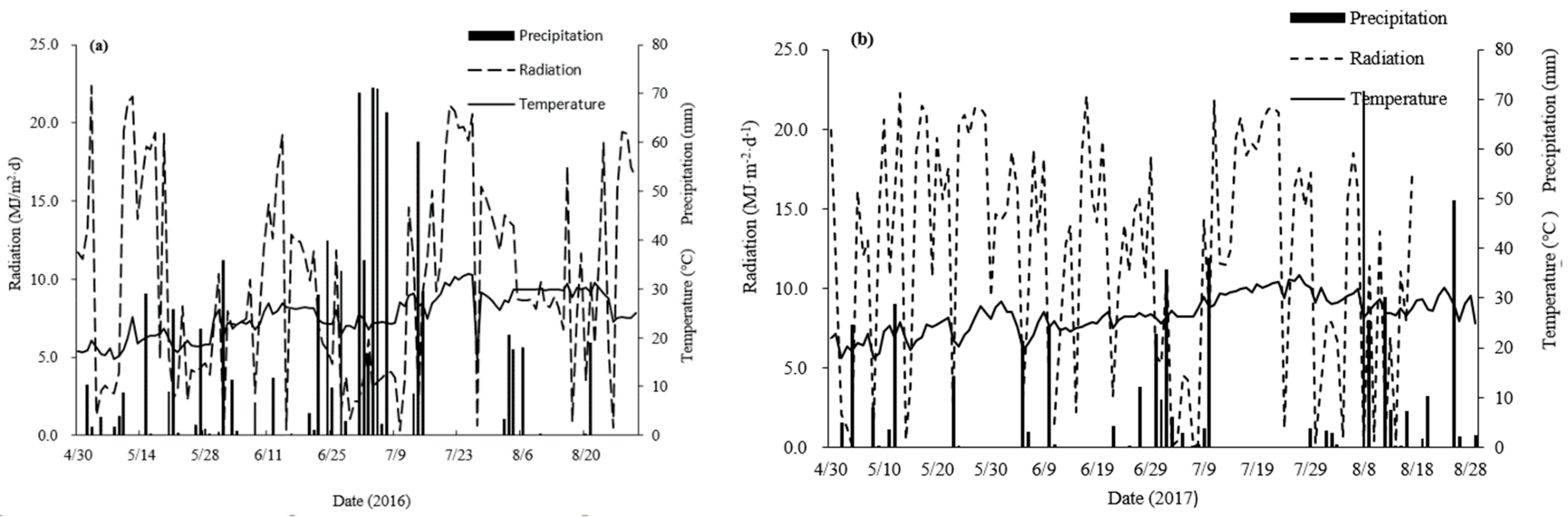
Figure 1 shows the variations in meteorological elements during the rice season of 2016 and 2017, respectively. From May to September 2016, the total precipitation was 815.0 mm, of which the precipitation time was mainly concentrated in the first 10 days of July, and the total radiation and average temperature were 1202.8 MJ/m2 and 24.6 °C, respectively. From May to September 2017, the total precipitation was 485.5 mm, and the total radiation and average temperature were 1472.2 MJ/m2 and 26.7 °C, respectively.
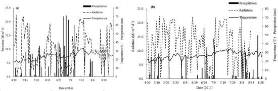
Figure 1.
The temporal variations in meteorological elements (radiation, precipitation, and temperature) at the station in 2016 (a) and 2017 (b), respectively.
Two shading treatments (T1 and T2) were set up in the experiment. After transplanting, two different shading materials were used to shade the rice until harvest. Each treatment was repeated 3 times with a random block design. The area of each experimental plot was 3 m × 3 m, and the interval between plots was 2 m. In each treatment, the shading material effectively covered 4 m2 and was dynamically adjusted to keep 0.6 m above the canopy. The radiation transmittance rate and diffuse radiation for each treatment are shown in Table 1. The diffuse radiation and total radiation were measured by the solar radiation monitor SPN1 (SPN1-MS1, Dalta-T, Inc., Cambridge, UK). The diffuse radiation and total radiation of each treatment were repeatedly measured 10 times, and the measurement data were tested for significance with a least significant difference (LSD) test (p < 0.05). The test results are outlined in Table 1. It is shown that, for the total radiation, CK was significantly different from T1 and T2, but there was no difference between T1 and T2, and for the diffuse radiation fraction, there were significant differences between CK, T1, and T2. Under these treatments, the rice experienced distinct radiation conditions, which helped to effectively simulate the growth of rice under an environment with changing radiation, as well as to determine the changes in LAI, SPAD, and hyperspectral reflectance characteristics.

Table 1.
Data of shading treatments.
2.2. Experimental Measurements
All canopy spectra were measured with an ASD FieldSpec Pro spectrometer (Analytical Spectral Devices, Boulder, CO, USA). This spectrometer is fitted with a 25° field of view, which operates in the 350–2500 nm spectral range, with sampling intervals of 1.4 nm between 350 nm and 1050 nm, and 2 nm between 1050 nm and 2500 nm. The spectrometer was calibrated using the whiteboard before the measurement. The measurements were made from a height of 0.6 m above the rice canopy under clear sky conditions between 9:00 a.m. and 11:00 a.m. on the 14th, 21st, and 28th day after rice heading (DAH 14d, DAH 21d, and DAH 28d; DAH means “days after heading”.).
Meanwhile, three samples from each plot were selected for measuring LAI and SPAD. During the measurement, the instruments LI-3000C and SPAD-502 Plus were employed, and flag leaves were selected for the SPAD measurement. Three flag leaves of rice were randomly selected to measure SPAD in each plot, and there were nine SPAD measurement data in the same period for each treatment. Three rice plants were also randomly selected to measure the LAI of rice in each plot.
2.3. Data Analysis
2.3.1. Parameters of Red Edge
The canopy reflectance spectra in the domain 680–760 nm are called “red edge”. The red edge, which contains considerable information and has a strong correlation with the chlorophyll abundance, nitrogen concentration, and leaf area index, can well characterize the growth status of rice. In general, there are two ways to derive red-edge parameters from red-edge reflectance spectra.
In the first method, a first-derivative curve of the spectra at the red edge was retrieved by Equation (1). The maximum value at this curve is defined as the red-edge amplitude (), and the corresponding wavelength is the red-edge position (). The integral area of the first-derivative curve at the red edge is defined as the red-edge area (). , , and are red-edge parameters.
where is the i-th wavelength, is the reflectance corresponding to the i-th wavelength, and is the first-derivative reflectance corresponding to the i-th wavelength.
In the second method, the inverse Gaussian model [45] was applied to derive since the model can fit the shape of the reflectance curve at the red edge well.
In Equation (2), is the wavelength, and is the reflectance. Rs is the maximum reflectance in the near-infrared range. R0 is the minimum reflectance in the red-light range. In this paper, the average reflectance in 780–795 nm and 670–675 nm was set as Rs and R0, respectively. In the above equation, and represent the red-edge position and the red-edge absorption band width, respectively. Both values were derived from an optimized Equation (2), with and data used as input.
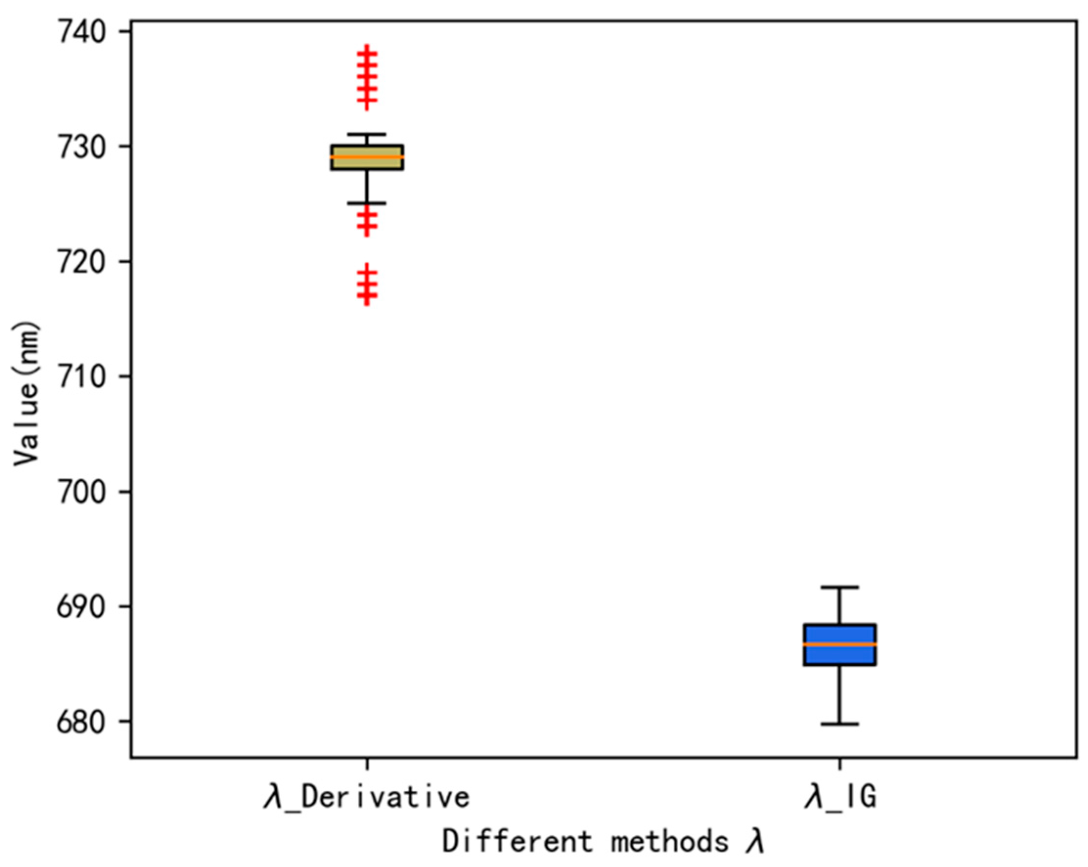
In this paper, the two methods were used separately to calculate . The results are presented in the box plots shown in Figure 2. From the figure, it can be seen that the average value of (728 nm) estimated by the first method was higher than the value of (687 nm) by the second method, but many outliers resulted from the first method. Against the possible high uncertainty in the further analysis, we chose the estimate by the second method as the default value of in this paper.
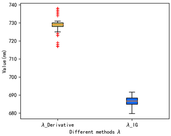
Figure 2.
Box plots of the estimated .
2.3.2. Parameters of Absorption Features
The absorption features of the rice canopy spectral curve are also important in analyzing the absorption characteristics for radiation. The baseline normalization method [28] was used to calculate the absorption features parameters of the spectral curve (Figure 3). To implement the method, points of local maximum on the spectral curve were detected first. With these points, linear interpolation was used to retrieve a linear upper envelope (Figure 3a). Afterward, by dividing the linear upper envelope, the normalized spectral curve was obtained from the canopy spectral curve (Figure 3b).
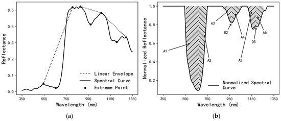
Figure 3.
Illustration of deriving values of the absorption features parameters: (a) shows the process of retrieving upper envelope of the spectral curve; (b) shows the normalized spectral curve and the absorption features parameters.
The normalized spectral curve contains three ordered absorption bandsfrom 350 nm to 1350 nm. The absorption bandparameters (A1, A2, A3, D2, A4, A5, D3, A6) were calculated using the method in Table 2. Detailed information about these parameters can be found in Figure 3b.
Table 2.
The description and calculation method of each absorption band parameter.
2.3.3. Statistical Analysis
Pearson’s correlation coefficient (R) [46,47], which is calculated with Equation (3), was used to analyze the correlation between SAPD, LAI, and the spectral parameter. A strong correlation between SPAD, LAI, and the spectral parameter could be observed if the absolute value of R was high.
where is a spectral parameter, which includes the spectral reflectance, red-edge parameters, and absorption features parameters. is the average of all spectral parameters. is the rice physiological indices, which include SPAD and LAI. is the average value of the rice physiological indices. m is the sample size.
For the Pearson’s correlation coefficient, we focused on statistical inference with the aim to test the null hypothesis, through which the true correlation coefficient is equal to 0, based on the value of the sample correlation coefficient R [46]. Then, we used the exact distribution to calculate the p-value—namely, when the samples x and y follow the normal distribution, the probability density function of the correlation coefficient R distribution can be calculated by Equation (4), while the p-value can be estimated using Equation (5). Generally, the smaller the p-value is, the more significant the correlation is. In this paper, 0.05 was used as the standard for significant correlation.
where R is the correlation coefficient, m is the sample size, and B represents the Beta distribution.
Two scientific computing languages—R 4.1.0 and Python 3.7.1—were used for all the above-mentioned modeling and data analysis. Furthermore, The LSD test was used to test the significance of the difference between treatments. The LSD test is used in the context of the analysis of variance when the F ratio suggests rejection of the null hypothesis H0, that is, when the difference between the population means is significant [48].
3. Results
3.1. The SPAD between Different Experimental Treatments
The SPAD of different treatments is shown in Table 3. It shows that the SPAD of T1 and T2 were generally higher than that of CK. Compared with CK, SPAD of T1 increased by 3.92%, 2.11%, and 1.20% at DAH 14d, DAH 21d, and DAH 28d (2016, p < 0.05, the same below), respectively. The average SPAD of T1 and T2 were close (39.74 for T1 and 40.53 for T2), but compared with T1, SPAD of T2 increased by 2.31%, 2.18%, and 1.30% at DAH 14d, DAH 21d, and DAH 28d, respectively, which could be due to the higher diffuse radiation fraction in T2. In addition, the largest difference of SPAD between T2 and T1 appeared at DAH 14d and then decreased after heading. The distribution of SPAD in 2016 and 2017 was also analyzed, which showed that the distribution was consistent. The above results suggest that the increase in the diffuse radiation fraction promotes the increase in rice SPAD.
Table 3.
The SPAD of rice under different treatments at different periods after heading in 2016–2017.
3.2. The LAI Values between Different Experimental Treatments
The LAI values of different treatments are shown in Table 4. Compared with CK, the LAI of T1 and T2 increased significantly. For instance, the LAI of T1 increased by 4.58%, 3.30%, and 3.86% at DAH 14d, DAH 21d, and DAH 28d, respectively. Furthermore, the average values of LAI for T1 and T2 in different periods were 5.03 and 5.42, respectively. Compared with T1, the LAI of T2 increased by 7.62%, 7.39%, and 8.06% at DAH 14d, DAH 21d, and DAH 28d, respectively. It was also found that the distribution of LAI in 2017 was consistent with 2016. The behavior of the change in LAI under the shading treatment indicates that an increase in diffuse radiation fraction led to an increase in rice LAI.
Table 4.
The LAI values of rice under different treatments at different periods after heading, in 2016–2017.
3.3. The Canopy Spectral Characteristics between Different Experimental Treatments
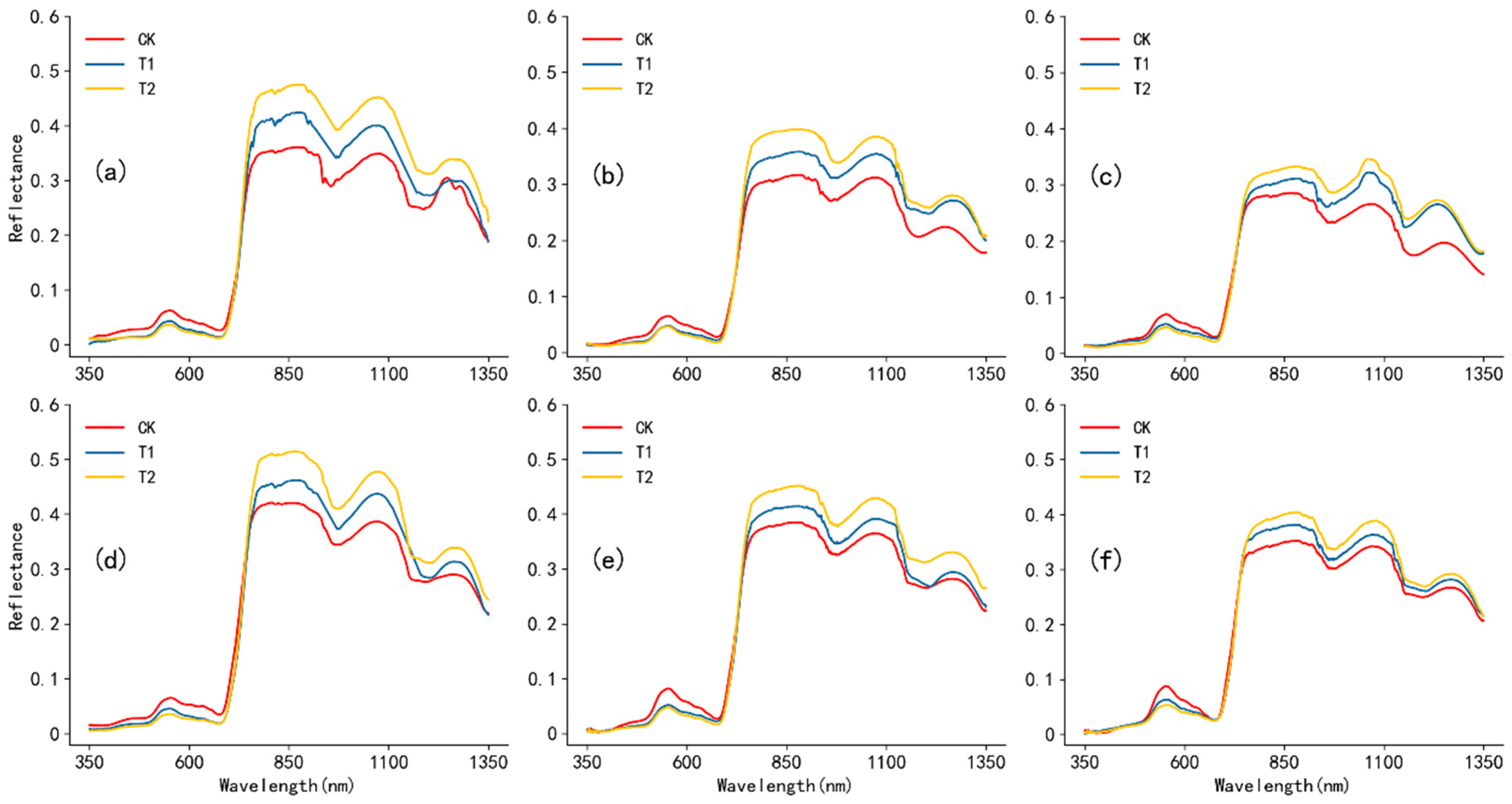
The canopy spectral curves of rice at different days after heading are shown in Figure 4. There was low reflectance in the visible region (350–760 nm), and its maximum reflectance appeared at near 550 nm (the green peak). In the near-infrared region (800–1350 nm), the reflectance was high, and there were a plateau region (800–900 nm) and two absorption bands at the spectral curve. It can be inferred from Figure 4 that the reflectances of T1 and T2 in the visible region were lower than that of CK, but the reflectances of T1 and T2 in the near-infrared region were higher than that of CK. The reflectances of T1 and T2 had a significant difference, and compared with T1, the reflectance of T2 decreased in the visible region and increased in the near-infrared region, which could be because of the higher diffuse radiation fraction in T2. Moreover, the largest difference of spectral curves between T2 and T1 appeared at DAH 14d, when the green peak reflectance of T2 decreased by 16.12% (2016), 21.34% (2017), and the average reflectance of T2 at plateau region (800–900 nm) increased by 10% (2016), 11% (2017). The analysis results suggest that an increase in diffuse radiation fraction led to a decrease in reflectance in the visible region and an increase in reflectance in the near-infrared region.
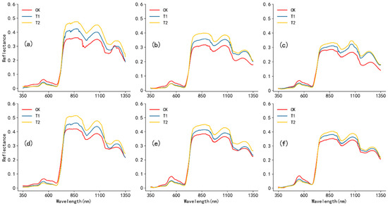
Figure 4.
Canopy spectra curves of rice between different treatments: (a–c) are DAH 14d, DAH 21d, and DAH 28d in 2016; (d–f) are DAH 14d, DAH 21d, and DAH 28d in 2017.
3.4. The Characteristics of the Canopy Red-Edge Spectra
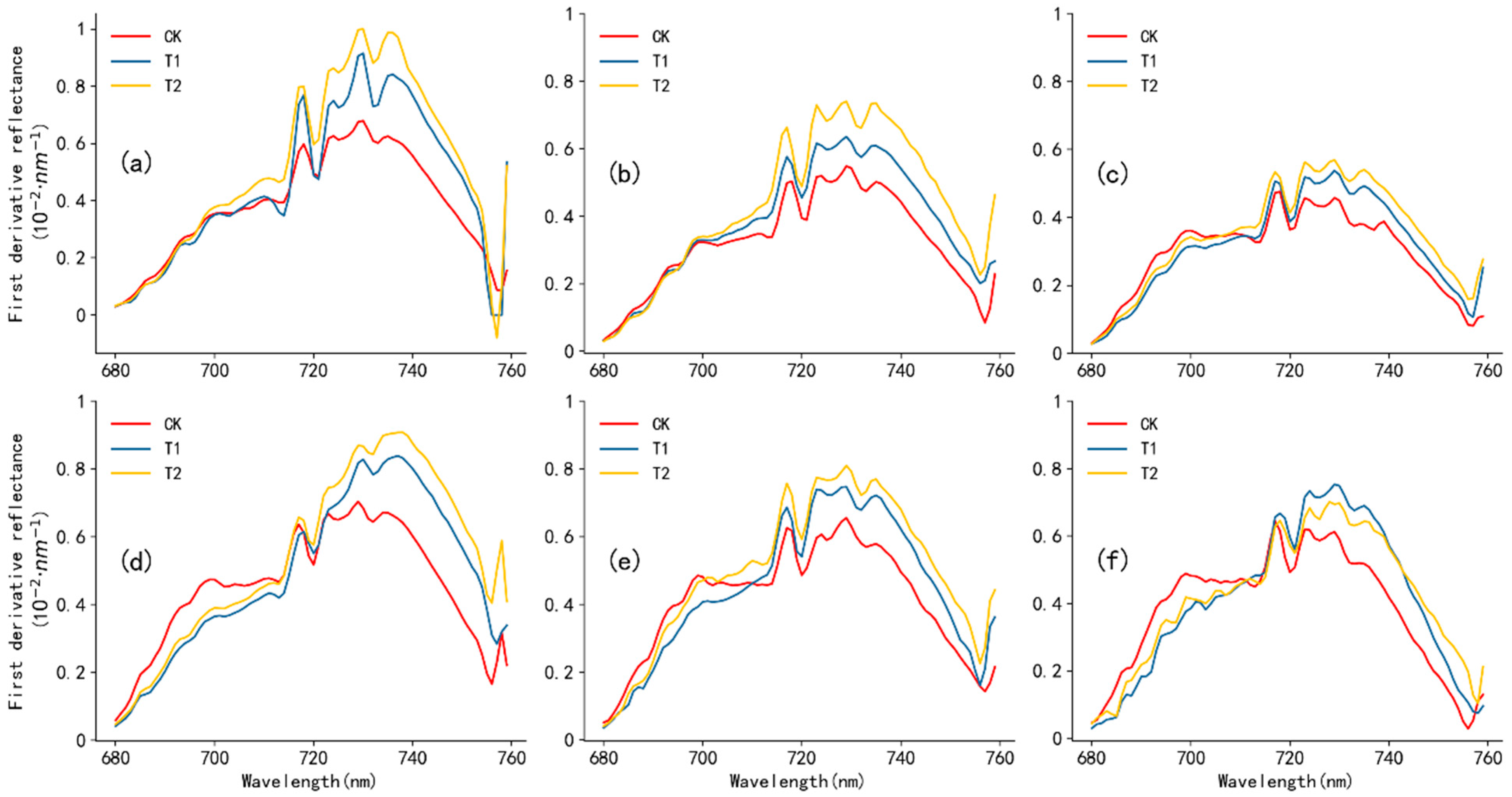
Figure 5 shows the first derivative for the red-edge reflectance spectra averaged over each of the treatments. There was a clear platform region at 700 nm–715 nm and a double peak, with existing multiple small peaks on the second peak, at 716 nm–740 nm. As the days after heading increased, the phenomenon of double peak became more significant, and the first derivative reflectance decreased gradually. The largest difference region of the first derivative reflectance spectra between T1 and T2 was in the double peak region, where the first derivative reflectance averaged over all the treatments of T2 was 16% higher than that of T1 (2016).
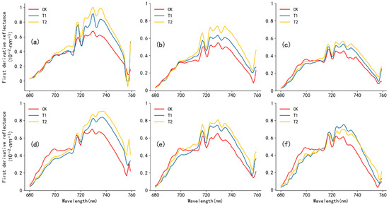
Figure 5.
The first derivative spectra curve of the red edge with different treatments: (a–c) are DAH 14d, DAH 21d, and DAH 28d in 2016; (d–f) are DAH 14d, DAH 21d, and DAH 28d in 2017.
More detailed information about the red edge can be gained from Table 5, which lists the red-edge parameters (, , , and ) under different treatments. Compared with CK, it shows that the of T1 and T2, with a value in the range of 685–690 nm, shifted toward the long-wavelength region of the spectra. However, there was no significant difference of between T1 and T2. The of T1 and T2 were generally higher than that of CK. The value of T1 and T2 were in the range of 0.0054–0.01 nm−1, and compared with T1, of T2 increased by 8.70%, 17.19%, and 7.41% at DAH 14d, DAH 21d, and DAH 28d (2016). The of T1 and T2, with a value in the range of 0.25–0.43, was also higher than that of CK. Compared with T1, the of T2 increased by 13.89%, 13.33%, and 12.00% at DAH 14d, DAH 21d, and DAH 28d (2016). The has no obvious change among all treatments. The distribution of red-edge parameters in 2016 and 2017 was also analyzed, which showed that the distribution was consistent. The results show that an increase in diffuse radiation fraction led to an increase in parameters and .
Table 5.
Red-edge parameters of rice canopy spectra between different treatments.
3.5. Analysis of Absorption Feature Parameters
The absorption features parameters between the different treatments are shown in Table 6. Compared with CK, the parameters A1, A2, A4, D2, A5, and D3 of T1 and T2 decreased significantly. There were also remarkable differences in absorption features between T1 and T2. The area of the first absorption feature of T2 was lower than that of T1. For instance, compared with T1, the parameter A1 of T2 decreased by 6.34%, 9.21%, and 7.82%, while A2 of T2 decreased by 8.11%, 4.43%, and 4.40% at DAH 14d, DAH 21d, and DAH 28d (2016), respectively. It was also found that the area of the right part and depth of the second absorption feature of T2 were lower than those of T1. Compared with T1, the parameter A4 of T2 decreased by 9.21%, 5.66%, and 18.11%, while D2 of T2 decreased by 20.59%, 13.79%, and 8.33% at DAH 14d, DAH 21d, and DAH 28d (2016), respectively. Furthermore, the area of the left part and depth of the third absorption feature of T2 were lower than those of T1. More specifically, compared with T1, A5 of T2 decreased by 10.90%, 14.20%, and 4.58%, while D3 of T2 decreased by 15.38%, 18.18%, and 23.81% at DAH 14d, DAH 21d, DAH 28d (2016), respectively. The distribution of absorption features in 2017 was also analyzed, which was consistent with that in 2016. All results suggest that an increase in diffuse radiation fraction could change the absorption features of the rice canopy remarkably.
Table 6.
Absorption feature parameters of rice canopy spectra curve under different treatments.
4. Discussion
Shao and Shin et al. indicate that shading treatment will increase the SPAD and LAI values of rice [49,50], which is consistent with the experimental results (CK compared with T1 and T2) presented in this paper. In summary, the shading treatment caused a decline in rice canopy spectral reflectance in the visible region and an increase in the near-infrared region. It also increased red-edge parameter values of , , and . However, the treatment reduced the values of A1, A2, A4, D2, A5, and D3.
For the comparison of T1 and T2, when the diffuse radiation fraction improved, the SPAD and LAI values of rice increased significantly, and the rice canopy spectral reflectance also decreased in the visible region and increased in the near-infrared region. The hyperspectral reflectance of rice canopy in different wavelengths is affected by rice chlorophyll content, LAI, cell structure, leaf structure, etc. [51]. To determine the reasons for the changes in the rice canopy spectra under the increasing diffuse radiation fraction, the correlation and p-value between the rice SPAD, LAI, and the spectral reflectance in DAH 14d, DAH 21d, and DAH 28d were calculated, as shown in Figure 6.
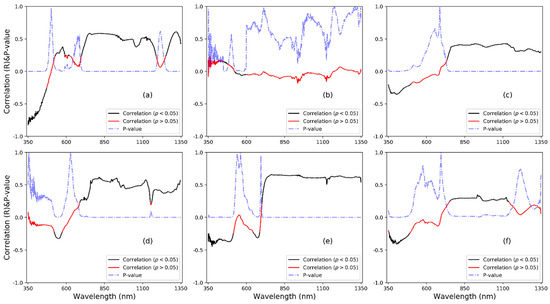
Figure 6.
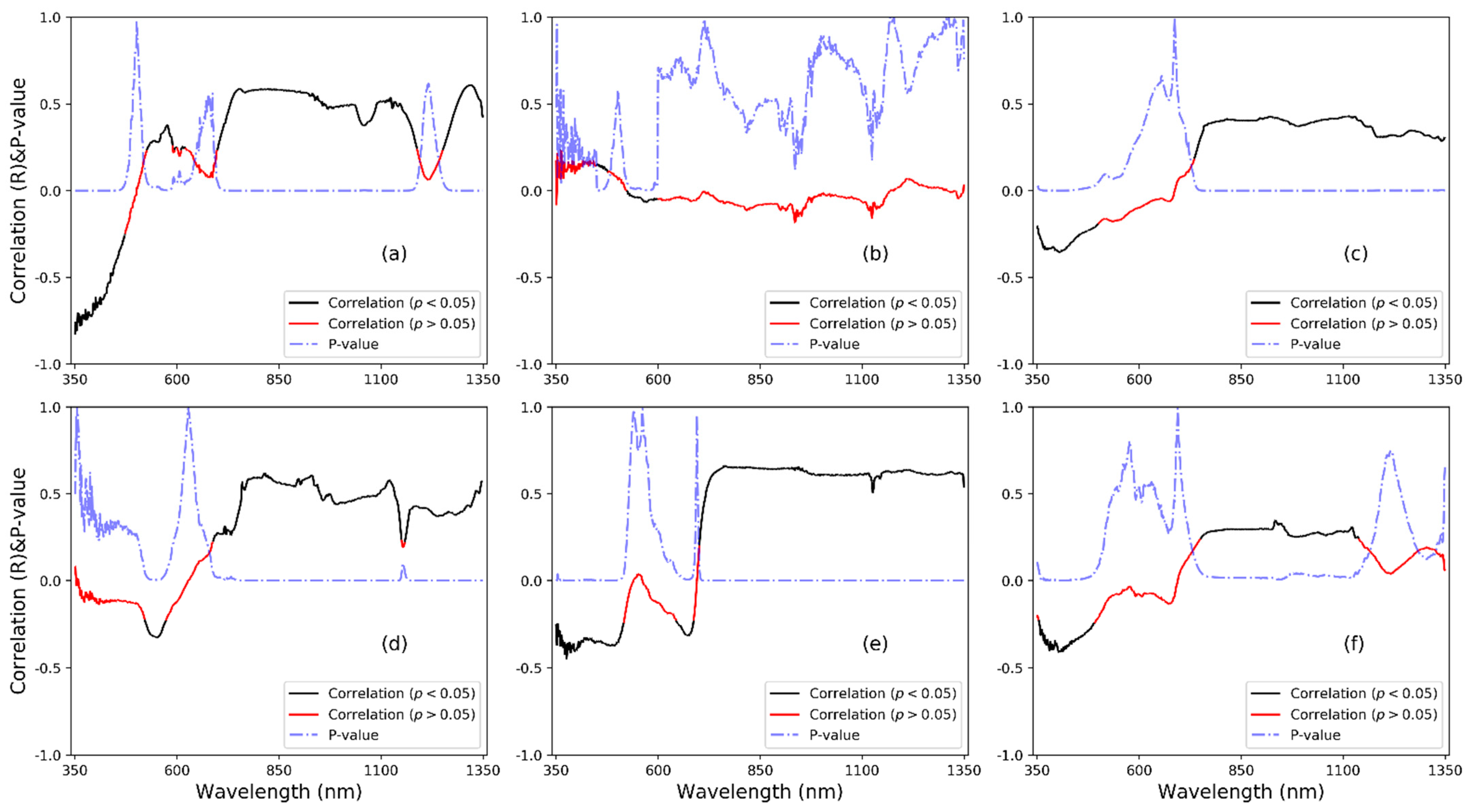
The correlation between SPAD, LAI and the spectral reflectance of T1 and T2 during 2016–2017: (a–c) are correlations of SPAD in DAH 14d, DAH 21d, and DAH 28d; (d–f) are correlations of LAI in DAH 14d, DAH 21d, and DAH 28d. The sample size for calculating Pearson’s correlation coefficient is 108.
Figure 6a,c show that the strongest negative correlation appeared at 355 nm (R = −0.79) in DAH 14d and 405 nm (−0.40) in DAH 28d. However, the correlation in DAH 21d did not pass the test of significance (Figure 6b). The rice SPAD was negatively correlated with the reflectance of the blue-violet light band. In other words, under the increasing diffuse radiation fraction, the increasing SPAD resulted in a stronger absorption of visible light. Li revealed that the shading treatment can lead to an increase in chlorophyll b [52], which is an important factor affecting the rice canopy spectra in the visible region [53,54]. This is consistent with the results presented in this paper.
Figure 6d–f show that the strongest positive correlation appeared at 814 nm (R = 0.62) in DAH 14d, 806 nm (0.66) in DAH 21d, and 934 nm (0.35) in DAH 28d. There was a strong positive correlation between the LAI value of rice and the spectral reflectivity in the near-infrared region. Therefore, under the increasing diffuse radiation fraction, the increasing LAI in rice led to increasing reflectivity in the near-infrared region [55,56]. In addition, the canopy spectra of T1 and T2 had the largest difference between 800 nm and 900 nm, which is affected by leaf and canopy structure [57]; that is, an increase in diffuse radiation fraction may cause changes in rice leaf and canopy structure [2].
The red-edge parameters of T1 and T2 had significant changes as the SPAD value of rice leaves changed [58,59]. The values of and area of T2 were greater than those of T1, with no significant difference in . However, Evri [60] pointed out that, without shading treatment, the red-edge parameter has a strong correlation with changes in rice SPAD, and the SPAD monitoring model based on has high accuracy, which indicates that when the diffuse radiation fraction increased, the model established with the red-edge parameters and area could have higher accuracy.
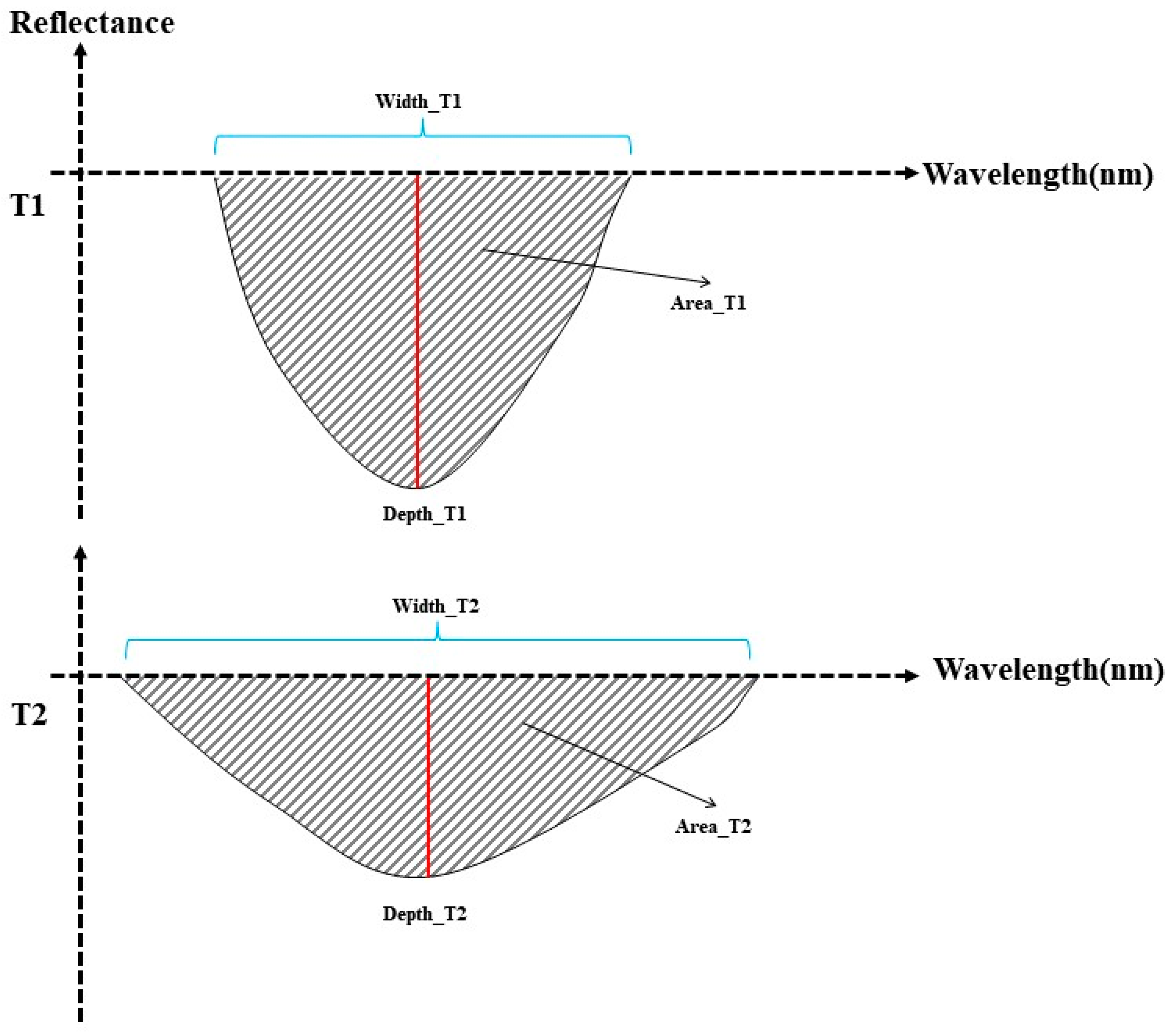
For the absorption features parameters, there was also a significant difference between T1 and T2. Under the increasing fraction of diffuse radiation, both parameters A1 and A2, which are the areas of the left and right of the first absorption band (the average wavelength was in the range of 553–788 nm.), decreased. The change in LAI, which has an impact on the shape of the first absorption band, is the main reason for the decrease in A1 and A2 [61]. The parameters A3, A4, and D2 are the left area, right area, and the depth of the second absorption band. Additionally, the parameters A5, A6, and D3 are the left area, right area, and the depth of the third absorption band. The results from Table 6 show that the parameter values of A4, A5, D2, and D3 of T2 experienced a significant decline when compared with T1. In addition, the normalized widths of the second and third absorption bands (W1, W2) calculated with Equations (6) and (7), shown in Table 7, reveal that there was a significant increase in parameter values of W1 and W2 of T2. For example, in comparison with T1, W1 of T2 increased by 17.50% and 11.16% at DAH 14d and DAH 21d (2016), respectively, and W2 increased by 7.87%, 11.76%, and 30.77% at DAH 14d, DAH 21d, and DAH 28d, respectively. In general, the depth and area of the second and third absorption band of T2 significantly reduced, but the width increased. The difference in absorption band shape between T1 and T2 is shown in Figure 7. In fact, the second and third absorption bands (the average wavelength was in the range of 874–1257 nm) are mainly affected by water vapor absorption [62,63,64]. Therefore, an increasing diffuse radiation fraction could also affect the water vapor absorption process of rice.
Table 7.
Normalized widths of the second and third absorption bands in T1 and T2.
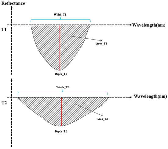
Figure 7.
Schematic diagram of the morphological changes of the second and third absorption bands on T1 and T2.
It is shown that an increase in diffuse radiation fraction had a positive effect on rice growth, including an increase in LAI, population photosynthesis capacity, and yield [13,17,18,19,43], which is also the reason for the changes in canopy spectra and red-edge parameters in this experiment.
5. Conclusions
In this paper, we analyzed the changes of SPAD, LAI, and canopy spectral characteristics of rice under increasing diffuse radiation fraction. The results show that the increase in diffuse radiation fraction led to the increase in SPAD and LAI of rice. Additionally, the reflectivity of canopy spectra in the visible light region decreased, while that in the near-infrared region increased. The absorption features, calculated with the baseline normalization method, changed remarkably as the diffuse radiation fraction increased. The correlation between spectral parameters and SPAD and LAI of rice was analyzed, and it seems more accurate monitoring models of SPAD and LAI values in rice under changes in the diffuse radiation fraction can be established based on the results of this paper. Further analysis of the different morphology of the canopy spectra between T1 and T2 shows that the increase in the diffuse radiation fraction will also affect the structure of rice leaf and canopy and the process of water vapor absorption. Building on this paper, in the future, the spectral parameters, which were highly correlated with SPAD and LAI in this paper, will be used to establish rice monitoring models with high accuracy and efficiency. Further, these models can be used in hyperspectral images to analyze the impact of increasing the diffuse radiation fraction on rice in large geographic regions. In addition, more rice field experiments should be designed to analyze the influence of increasing the diffuse radiation fraction on the water vapor absorption process of rice.
Author Contributions
Conceptualization, T.Z. and X.J.; methodology, T.Z. and X.J.; investigation, L.J. and X.L.; formal analysis, L.J. and X.L.; writing—original draft preparation, T.Z. and X.J.; writing—review and editing, T.Z., X.J., S.Y., and Y.L. All authors have read and agreed to the published version of the manuscript.
Funding
This research was funded by the National Natural Science Foundation of China, Grant Number 41875140, the National Key Research and Development Program of China, Grant Number 2019YFD1002202, and the Special Fund for Meteorological Scientific Research in the Public Welfare of China, Grant Number GYHY201506018.
Institutional Review Board Statement
Not applicable.
Informed Consent Statement
Not applicable.
Data Availability Statement
The data presented in this study are available on request from the corresponding author.
Conflicts of Interest
The authors declare no conflict of interest.
References
- Stanhill, G.; Cohen, S. Global dimming: A review of the evidence for a widespread and significant reduction in global radiation with discussion of its probable causes and possible agricultural consequences. Agric. For. Meteorol. 2001, 107, 255–278. [Google Scholar] [CrossRef]
- Knohl, A.; Baldocchi, D.D. Effects of diffuse radiation on canopy gas exchange processes in a forest ecosystem. J. Geophys. Res. Biogeosciences 2008, 113, G02023. [Google Scholar] [CrossRef]
- Qian, Y.; Kaiser, D.P. More frequent cloud-free sky and less surface solar radiation in China from 1955 to 2000. Geophys. Res. Lett. 2006, 33, L01812. [Google Scholar] [CrossRef] [Green Version]
- Wang, K.; Dickinson, R.E. Clear sky visibility has decreased over land globally from 1973 to 2007. Science 2009, 323, 1468–1470. [Google Scholar] [CrossRef]
- Ren, X.L.; He, H.L. Spatiotemporal variability analysis of diffuse radiation in China during 1981–2010. Ann. Geophys. Copernic. GmbH 2013, 31, 277–289. [Google Scholar] [CrossRef] [Green Version]
- Xie, H.; Zhao, J. Long-term variations in solar radiation, diffuse radiation, and diffuse radiation fraction caused by aerosols in China during 1961–2016. PLoS ONE 2021, 16, e0250376. [Google Scholar] [CrossRef] [PubMed]
- Xue, W.; Zhang, J. Spatiotemporal variations and relationships of aerosol-radiation-ecosystem productivity over China during 2001–2014. Sci. Total. Environ. 2020, 741, 140324. [Google Scholar] [CrossRef]
- IPCC. Climate Change 2013: The Physical Science Basis: Working Group I Contribution to the Fifth Assessment Report of the Intergovernmental Panel on Climate Change; Cambridge University Press: Cambridge, UK, 2014. [Google Scholar]
- Xu, H.; Guo, J. Warming effect of dust aerosols modulated by overlapping clouds below. Atmos. Environ. 2017, 166, 393–402. [Google Scholar] [CrossRef] [Green Version]
- Guo, J.; Lou, M. Trans-Pacific transport of dust aerosols from East Asia: Insights gained from multiple observations and modeling. Environ. Pollut. 2017, 230, 1030–1039. [Google Scholar] [CrossRef]
- Yang, X.; Li, J. Impacts of diffuse radiation fraction on light use efficiency and gross primary production of winter wheat in the North China Plain. Agric. For. Meteorol. 2019, 275, 233–242. [Google Scholar] [CrossRef]
- Black, K.; Davis, P. Long-term trends in solar irradiance in Ireland and their potential effects on gross primary productivity. Agric. For. Meteorol. 2006, 141, 118–132. [Google Scholar] [CrossRef]
- Kanniah, K.D.; Beringer, J. Control of atmospheric particles on diffuse radiation and terrestrial plant productivity: A review. Prog. Phys. Geogr. 2012, 36, 209–237. [Google Scholar] [CrossRef]
- Rap, A.; Scott, C.E. Enhanced global primary production by biogenic aerosol via diffuse radiation fertilization. Nat. Geosci. 2018, 11, 640–644. [Google Scholar] [CrossRef] [Green Version]
- Proctor, J.; Hsiang, S. Estimating global agricultural effects of geoengineering using volcanic eruptions. Nature 2018, 560, 480–483. [Google Scholar] [CrossRef]
- Schiferl, L.D.; Heald, C.L. Particulate matter air pollution may offset ozone damage to global crop production. Atmos. Chem. Phys. 2018, 18, 5953–5966. [Google Scholar] [CrossRef] [Green Version]
- Mercado, L.M.; Bellouin, N. Impact of changes in diffuse radiation on the global land carbon sink. Nature 2009, 458, 1014–1017. [Google Scholar] [CrossRef] [Green Version]
- Jiang, X.-D.; Chen, H.-L. Effect of increasing diffuse radiation fraction under low light condition on the grain-filling process of winter wheat (Triticum aestivum L.). Chin. J. Agrometeorol. 2017, 38, 753. (In Chinese) [Google Scholar]
- Zheng, B.Y.; Ma, Y.T. Assessment of the influence of global dimming on the photosynthetic production of rice based on three-dimensional modeling. Sci. China Earth Sci. 2011, 54, 290–297. (In Chinese) [Google Scholar] [CrossRef]
- Sahoo, R.N.; Ray, S.S. Hyperspectral remote sensing of agriculture. Curr. Sci. 2015, 108, 848–859. [Google Scholar]
- Jensen, J.R. Remote Sensing of the Environment: An Earth Resource Perspective; Pearson Education India: Bengaluru, India, 2009. [Google Scholar]
- Sun, Q.; Gu, X. Dynamic change in rice leaf area index and spectral response under flooding stress. Paddy Water Environ. 2020, 18, 223–233. [Google Scholar] [CrossRef]
- Xie, X.J.; Li, Y.X. Hyperspectral characteristics and growth monitoring of rice (Oryza sativa) under asymmetric warming. Int. J. Remote. Sens. 2013, 34, 8449–8462. [Google Scholar] [CrossRef]
- Xie, X.J.; Zhang, Y.H. Prediction model of rice crude protein content, amylose content and actual yield under high temperature stress based on hyper-spectral remote sensing. Qual. Assur. Saf. Crop. Foods 2019, 11, 517–527. [Google Scholar] [CrossRef]
- Liu, C.; Hu, Z. Hyperspectral characteristics and leaf area index monitoring of rice (Oryza sativa L.) under carbon dioxide concentration enrichment. Spectrosc. Lett. 2021, 54, 231–243. [Google Scholar] [CrossRef]
- Viña, A.; Gitelson, A.A. Comparison of different vegetation indices for the remote assessment of green leaf area index of crops. Remote. Sens. Environ. 2011, 115, 3468–3478. [Google Scholar] [CrossRef]
- Liang, L.; Di, L. Estimation of crop LAI using hyperspectral vegetation indices and a hybrid inversion method. Remote Sens. Environ. 2015, 165, 123–134. [Google Scholar] [CrossRef]
- Kokaly, R.F. Investigating a physical basis for spectroscopic estimates of leaf nitrogen concentration. Remote Sens. Environ. 2001, 75, 153–161. [Google Scholar] [CrossRef]
- Herrmann, I.; Pimstein, A. LAI assessment of wheat and potato crops by VENμS and Sentinel-2 bands. Remote Sens. Environ. 2011, 115, 2141–2151. [Google Scholar] [CrossRef]
- Fan, W.J.; Xu, X.R. Accurate LAI retrieval method based on PROBA/CHRIS data. Hydrol. Earth Syst. Sci. 2010, 14, 1499–1507. [Google Scholar] [CrossRef] [Green Version]
- Fu, Y.; Yang, G. Winter wheat biomass estimation based on spectral indices, band depth analysis and partial least squares regression using hyperspectral measurements. Comput. Electron. Agric. 2014, 100, 51–59. [Google Scholar] [CrossRef]
- Dong, T.; Liu, J. Deriving maximum light use efficiency from crop growth model and satellite data to improve crop biomass estimation. IEEE J. Sel. Top. Appl. Earth Obs. Remote Sens. 2016, 10, 104–117. [Google Scholar] [CrossRef]
- Stroppiana, D.; Boschetti, M. Plant nitrogen concentration in paddy rice from field canopy hyperspectral radiometry. Field Crop. Res. 2009, 111, 119–129. [Google Scholar] [CrossRef]
- Cheng, T.; Song, R. Spectroscopic estimation of biomass in canopy components of paddy rice using dry matter and chlorophyll indices. Remote Sens. 2017, 9, 319. [Google Scholar] [CrossRef] [Green Version]
- Wang, L.; Chang, Q. Estimation of paddy rice leaf area index using machine learning methods based on hyperspectral data from multi-year experiments. PLoS ONE 2018, 13, e0207624. [Google Scholar] [CrossRef] [PubMed] [Green Version]
- Kanning, M.; Kühling, I. High-resolution UAV-based hyperspectral imagery for LAI and chlorophyll estimations from wheat for yield prediction. Remote Sens. 2018, 10, 2000. [Google Scholar] [CrossRef] [Green Version]
- Wang, L.; Chen, S. Phenology effects on physically based estimation of paddy rice canopy traits from UAV hyperspectral imagery. Remote Sens. 2021, 13, 1792. [Google Scholar] [CrossRef]
- Liang, L.; Geng, D. Estimating crop LAI using spectral feature extraction and the hybrid inversion method. Remote Sens. 2020, 12, 3534. [Google Scholar] [CrossRef]
- Zhang, B.; Sun, X. Endmember extraction of hyperspectral remote sensing images based on the ant colony optimization (ACO) algorithm. IEEE Trans. Geosci. Remote Sens. 2011, 49, 2635–2646. [Google Scholar] [CrossRef]
- Yuan, N.; Gong, Y. UAV remote sensing estimation of rice yield based on adaptive spectral endmembers and bilinear mixing model. Remote Sens. 2021, 13, 2190. [Google Scholar] [CrossRef]
- Chen, Y.; Jiang, H. Deep feature extraction and classification of hyperspectral images based on convolutional neural networks. IEEE Trans. Geosci. Remote Sens. 2016, 54, 6232–6251. [Google Scholar] [CrossRef] [Green Version]
- Hang, R.; Liu, Q. Cascaded recurrent neural networks for hyperspectral image classification. IEEE Trans. Geosci. Remote Sens. 2019, 57, 5384–5394. [Google Scholar] [CrossRef] [Green Version]
- Qin, A.; Shang, Z. Spectral–spatial graph convolutional networks for semisupervised hyperspectral image classification. IEEE Geosci. Remote Sens. Lett. 2018, 16, 241–245. [Google Scholar] [CrossRef]
- Hong, D.; Gao, L. Graph convolutional networks for hyperspectral image classification. IEEE Trans. Geosci. Remote Sens. 2020, 59, 5966–5978. [Google Scholar] [CrossRef]
- Miller, J.R.; Hare, E.W. Quantitative characterization of the vegetation red edge reflectance 1. An inverted-Gaussian reflectance model. Remote Sens. 1990, 11, 1755–1773. [Google Scholar] [CrossRef]
- Pearson Correlation Coefficient. Wikipedia. Available online: https://en.wikipedia.org/wiki/Pearson_correlation_coefficient. (accessed on 25 October 2021).
- Hotellings, H. New light on the correlation coefficient and its transforms. J. R. Stat. Soc. Ser. B (Methodol.) 1953, 15, 193–232. [Google Scholar] [CrossRef]
- Dodge, Y. The Concise Encyclopedia of Statistics; Springer: New York, NY, USA, 2008. [Google Scholar]
- Shao, L.; Li, G. The fertilization effect of global dimming on crop yields is not attributed to an improved light interception. Glob. Chang. Biol. 2020, 26, 1697–1713. [Google Scholar] [CrossRef]
- Shin, J.M.; Song, S.H. Effects of strong shading on growth and yield in sweet potato (Ipomoea batatas L. In LAMK.) In Proceedings of the Korean Society of Crop Science Conference, the Korean Society of Crop Science, Jeju, Korea, 5–7 June 2017; p. 241. [Google Scholar]
- Smith, R.B. Introduction to Remote Sensing of the Environment. 2001. Available online: http://www.microimages.com (accessed on 25 October 2021).
- Li, H.; Jiang, D. Effects of shading on morphology, physiology and grain yield of winter wheat. Eur. J. Agron. 2010, 33, 267–275. [Google Scholar] [CrossRef]
- An, G.; Xing, M. Estimating chlorophyll content of rice based on UAV-based hyperspectral imagery and continuous wavelet transform. In Proceedings of the IGARSS 2020—2020 IEEE International Geoscience and Remote Sensing Symposium, Waikoloa, HI, USA, 26 September–2 October 2020; pp. 5270–5273. [Google Scholar]
- Xu, X.; Gu, X. Assessing rice chlorophyll content with vegetation indices from hyperspectral data. In Proceedings of the International Conference on Computer and Computing Technologies in Agriculture, Nanchang, China, 22–25 October 2010; Springer: Berlin/Heidelberg, Germany, 2010; pp. 296–303. [Google Scholar]
- Duan, B.; Liu, Y. Remote estimation of rice LAI based on Fourier spectrum texture from UAV image. Plant Methods 2019, 15, 124. [Google Scholar] [CrossRef] [Green Version]
- Wang, F.; Huang, J. A comparison of three methods for estimating leaf area index of paddy rice from optimal hyperspectral bands. Precis. Agric. 2011, 12, 439–447. [Google Scholar] [CrossRef]
- Ren, W.J.; Yang, W.Y. Impact of low-light stress on leaves characteristics of rice after heading. J. Sichuan Agric. Univ. 2002, 20, 205–208. (In Chinese) [Google Scholar]
- Pei, H.; Li, C. Hyperspectral estimation methods for chlorophyll content of apple based on random forest. In Proceedings of the International Conference on Computer and Computing Technologies in Agriculture, Jilin, China, 12–15 August 2017; Springer: Cham, Switzerland, 2017; pp. 194–207. [Google Scholar]
- Liu, N.; Liu, G. Real-time detection on spad value of potato plant using an in-field spectral imaging sensor system. Sensors 2020, 20, 3430. [Google Scholar] [CrossRef]
- Evri, M.; Akiyama, T. Spectrum analysis of hyperspectral red edge position to predict rice biophysical parameters and grain weight. J. Jpn. Soc. Photogramm. Remote Sens. 2008, 47, 4–15. [Google Scholar] [CrossRef]
- Hennessy, A.; Clarke, K. Hyperspectral classification of plants: A review of waveband selection generalisability. Remote Sens. 2020, 12, 113. [Google Scholar] [CrossRef] [Green Version]
- Elvidge, C.D. Visible and near infrared reflectance characteristics of dry plant materials. Remote Sens. 1990, 11, 775–1795. [Google Scholar] [CrossRef]
- Schmidt, K.S.; Skidmore, A.K. Spectral discrimination of vegetation types in a coastal wetland. Remote Sens. Environ. 2003, 85, 92–108. [Google Scholar] [CrossRef]
- Wang, J.; Xu, R. Estimation of plant water content by spectral absorption features centered at 1450 nm and 1940 nm regions. Environ. Monit. Assess. 2009, 157, 459–469. [Google Scholar] [CrossRef] [PubMed]

Publisher’s Note: MDPI stays neutral with regard to jurisdictional claims in published maps and institutional affiliations. |
© 2022 by the authors. Licensee MDPI, Basel, Switzerland. This article is an open access article distributed under the terms and conditions of the Creative Commons Attribution (CC BY) license (https://creativecommons.org/licenses/by/4.0/).