Article

Unifying Deep ConvNet and Semantic Edge Features for Loop Closure Detection

School of Electrical and Information Engineering, Tianjin University, Tianjin 300072, China
*
Author to whom correspondence should be addressed.
Remote Sens. 2022, 14(19), 4885; https://doi.org/10.3390/rs14194885
Submission received: 24 August 2022 / Revised: 26 September 2022 / Accepted: 27 September 2022 / Published: 30 September 2022

Abstract

:
Loop closure detection is an important component of Simultaneous Localization and Mapping (SLAM). In this paper, a novel two-branch loop closure detection algorithm unifying deep Convolutional Neural Network (ConvNet) features and semantic edge features is proposed. In detail, we use one feature extraction module to extract both ConvNet and semantic edge features simultaneously. The deep ConvNet features are subjected to a Context Feature Enhancement (CFE) module in the global feature ranking branch to generate a representative global feature descriptor. Concurrently, to reduce the interference of dynamic features, the extracted semantic edge information of landmarks is encoded through the Vector of Locally Aggregated Descriptors (VLAD) framework in the semantic edge feature ranking branch to form semantic edge descriptors. Finally, semantic, visual, and geometric information is integrated by the similarity score fusion calculation. Extensive experiments on six public datasets show that the proposed approach can achieve competitive recall rates at 100% precision compared to other state-of-the-art methods.

Graphical Abstract

1. Introduction

With the rapid expansion of driverless cars and mobile robots such as Unmanned Aerial Vehicles (UAV) and Automated Guided Vehicles (AGV), etc., Simultaneous Localization and Mapping (SLAM) has attracted widespread attention from both academia and industry [1]. The vision sensor-based SLAM system usually consists of the following modules: front-end visual odometer, back-end nonlinear optimization, loop closure detection (LCD), and mapping [2]. Visual LCD aims to identify areas visited by the robot during its motion [3]. By accurately detecting previously visited locations and matching them, the accumulated position errors of the visual odometer can be effectively eliminated, thus ensuring the accuracy of the SLAM system even in long-term, wide-area navigation and localization [4].
An important aspect of improving visual LCD performance is to obtain effective scene descriptions based on the input images. Traditional LCD methods rely on hand-crafted feature descriptors for image matching. As an example of local features, each database image is represented using local invariant features, and the features are clustered into a fixed length vector, for example, bag of visual words (BoVW) [5], VLAD [6], or Fisher Vectors [7]. These descriptor methods have significant advantages in terms of efficiency, but they cannot represent complex structures and textures in images. They are susceptible to scene changes in dynamic environments and cannot satisfy the needs of robots working in complex environments [8].
In recent years, ConvNet-based feature extraction has gradually replaced the traditional hand-crafted feature extraction methods [9]. The original visual image is fed into a well-designed deep ConvNet network, from which the deep ConvNet features of the image are learned directly. LCD methods based on learned features have been proven to be faster, more accurate, and more robust to scene changes than traditional methods, as shown by Zhang et al. [10]. Although the learning-based approach achieves good performance on the trained dataset, its generalization ability while facing new environments still needs to be improved. Some works [11,12,13,14,15] built high-level semantic feature descriptors from the perspective of scene understanding. Abel et al. [11] proposed an X-View global positioning system that employed a semantic segmentation result map of images to generate topological descriptors and performed matching to accomplish place recognition and global positioning. Using semantic nodes as an abstract representation of landmarks can reduce the impact of appearance changes. Benbihi et al. [12] achieved place recognition by direct matching the semantic edges of two images in bucolic environments. These works were built based on semantic segmentation networks as image pre-processing modules, followed by semantic feature extraction and description. Different from the work mentioned above, we are interested in the impact of two kinds of different features. The abstract deep ConvNet features are widely used for their excellent performance in LCD tasks. Additionally, the complex human-understandable semantic edge features containing rich high-level semantic and geometric information help to improve the robustness of the system. By unifying both abstract ConvNet features and figurative semantic edge features, the pipeline enables an adequate description of image information.
In this paper, we propose a novel and efficient two-branch LCD algorithm. The inputs of the two branches are ConvNet features and multi-class semantic edges, respectively, generated by the feature extraction module which is stacked by multi-residual networks (Multi-ResNet). The ConvNet features are enhanced by the Context Feature Enhancement (CFE) module and finally generate a robust global feature representation. The extracted semantic edges are ranked with image similarity scores using the semantic edge descriptors constructed by the VLAD framework in the semantic edge feature ranking branch. The similarity scores of the two feature descriptors are input to the similarity scores fusion module for final LCD determination. To emphasize, we only need to perform once time-consuming feature extraction process, and the generated features can be shared by the two branches.
The main contributions of this paper are summarized as follows:
(1)
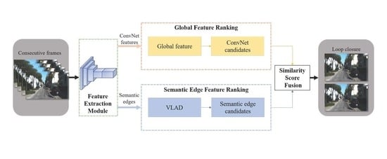
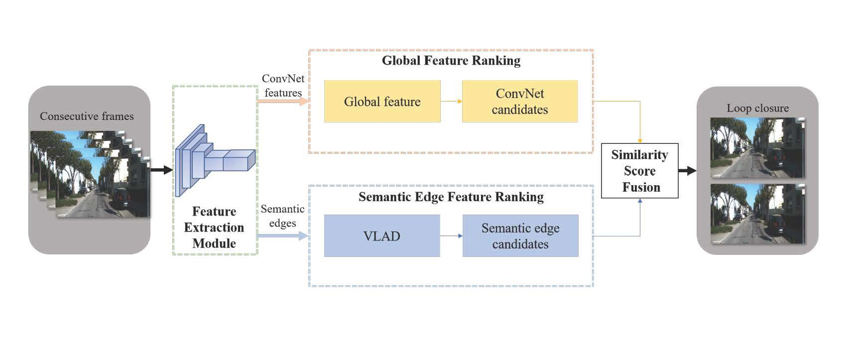
A two-branch network unifying ConvNet features and semantic edge features is proposed to improve the robustness of LCD.
(2)
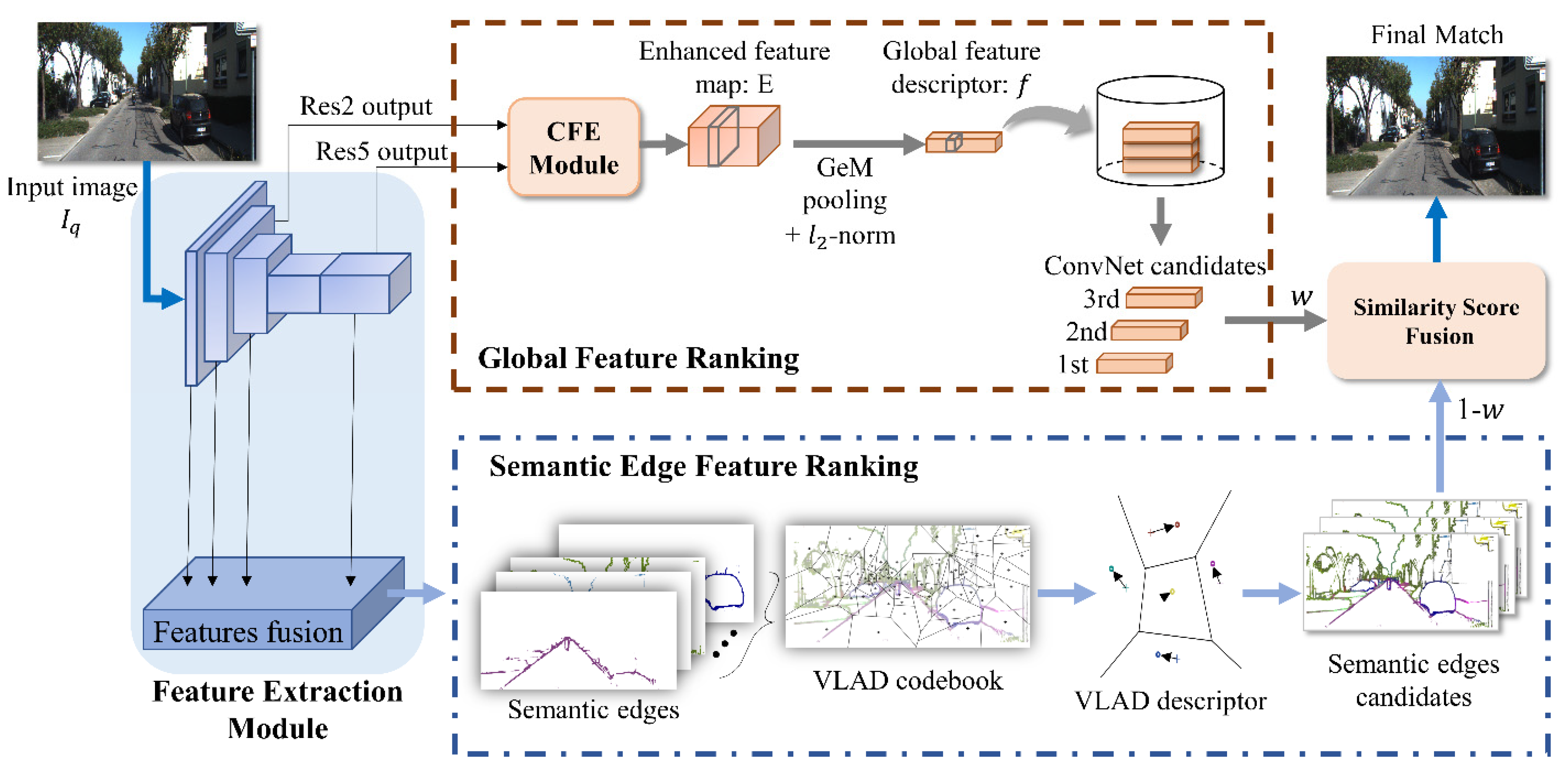
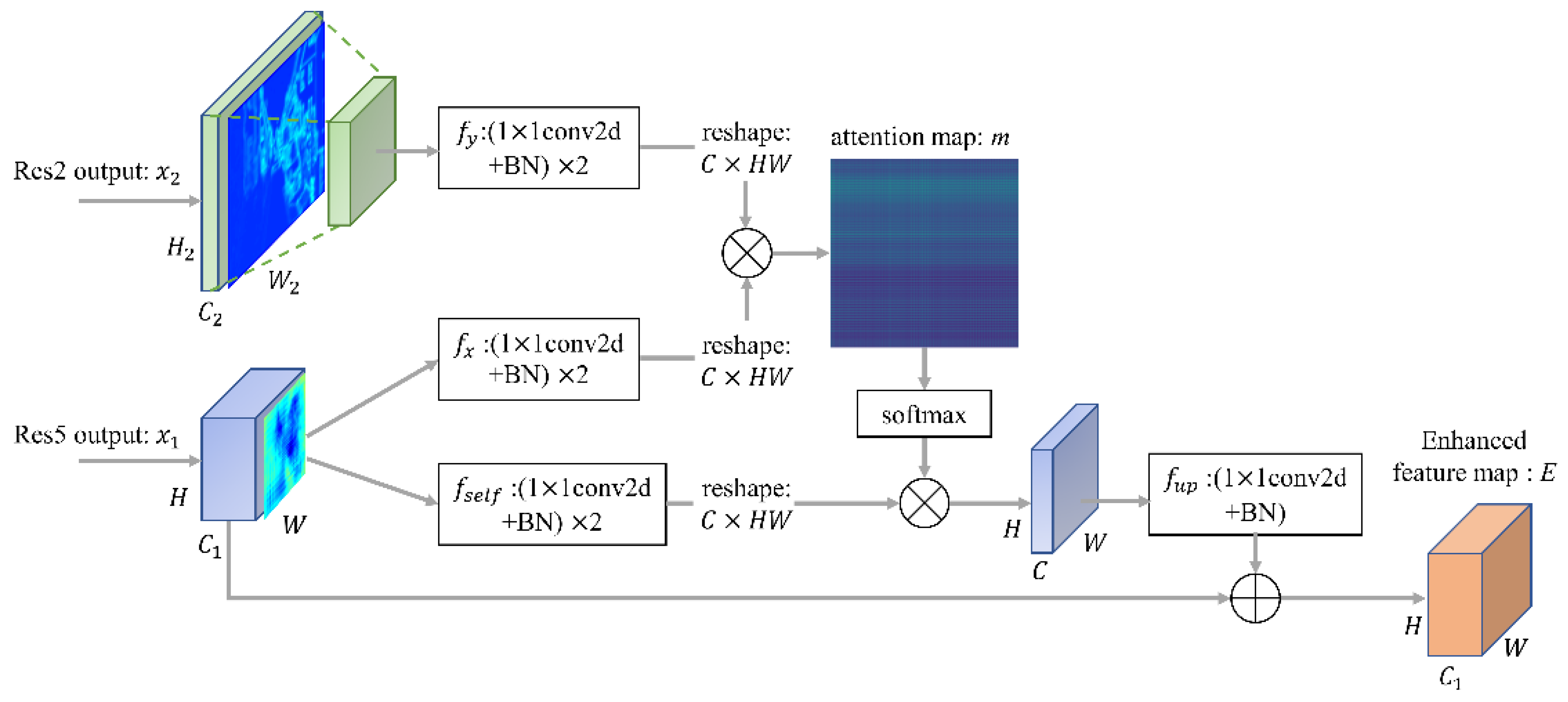
A CFE module using low-level boundary textures as mutual guidance for aggregating context information is designed to improve the robustness of the ConvNet feature descriptor.
(3)
Comparable experiments on six public challenging image sequences with state-of-the-art methods show that the proposed approach achieves competitive recall rates at 100% precision.
The rest of the paper is organized as follows. Section 2 summarizes related work in LCD and Section 3 describes the proposed algorithm in detail. In Section 4, experimental results and comparative algorithm are analyzed. Section 5 presents a discussion of the proposed algorithm. Finally, Section 6 concludes the study.

2. Related Work

LCD primarily relies on the extraction and representation of environmental information. There have been many different methods for encoding and mapping the images captured by the vision sensor. We divide previous works into two categories: using traditional hand-crafted features and ConvNet-based representations.

2.1. Hand-Crafted Features for LCD

For a long time, LCD task has been limited to hand-crafted feature-based representations. Hand-crafted features can be distinguished as global descriptors and local descriptors [8]. Gist [16] and Hog [17] descriptors are among the most acknowledged global descriptors, they encode viewpoint information through concatenation of grid cells and use a single vector to describe the overall appearance of the image. These methods have the advantage of compact representation and computational efficiency, but cannot handle occluded, viewpoint-changing scenes. The hand-crafted local feature extractor detects regions of interest in an image and describes them. FAB-MAP [18] is a probabilistic appearance-based method that extracts SIFT and SURF features from the database and clusters the features as a tree structure called visual dictionary. Bag-of-Binary-Words (BoBW) [19] constructs a visual dictionary using FAST and BRIEF binary descriptors and combines invariance to scale and rotation variations, thus obtaining excellent performance in terms of accuracy and efficiency. HTMap [20] is a two-level loop closure approach based on a hierarchical decomposition of the environment. Each image is represented using the pyramid histogram of oriented gradients (PHOG) global descriptor and a set of local features (LDB binary descriptor). This hierarchical scheme increases the speed of search while maintaining high accuracy. Tsintotas et al. [21] proposed an online image-to-sequence probabilistic voting framework, which is independent of any prior knowledge of the working environment. The same authors improved their approach named BoTW-LCD by adding a temporal filter and a vocabulary management technique to reduce the growth rate of the vocabulary and constraint the computational complexity of the system [22].

2.2. ConvNet-Based Features for LCD

The development of deep learning in the computer vision field provides more solutions for the LCD task. Lategahn et al. [23] proposed an Illumination Robust Descriptor (DIRD), using a meta-heuristic algorithm to train the descriptors and obtain better performance than hand-crafted descriptors. Subsequently, many methods started to use ConvNet as an encoder to obtain the overall representation of the image. Chen et al. [24] were the first to use a pre-trained ConvNet named Overfeat to learn image features for detecting similar localizations. FILD [25] uses ConvNet features extracted from the final average pooling layer of MobileNetV2 [26] as the image representation. Inspired by VLAD, the NetVLAD [27] network utilizes an end-to-end training architecture. The trained representation outperforms off-the-shelf ConvNet descriptors. Yu et al. [28] built a spatial pyramid-enhanced VLAD (SPE-VLAD) layer to encode feature extraction and trained the network with the weighted triplet loss (WT-loss). In addition, some approaches [29,30,31] used the attention mechanism to identify salient regions in the feature map to improve the performance of LCD tasks.
Different from the convolutional mapping employed by the above descriptors, another series of descriptors rely on the use of convolutional activation, more specifically, detecting semantic entities’ information in the image and aggregating them into a final representation. In [32], the semantic histogram and the HOG descriptors constructed using the pixel-level semantic labels of the query image were stacked into a final descriptor vector. VLASE [14] implemented vehicle localization using semantic edges. In particular, pixels located at semantic edges generated by the probability distribution of the last layer of the ConvNet were considered as entities of interest and aggregated into a VLAD descriptor. Benbihi et al. [12] designed a global image description applicable to bucolic environments across seasons. It was built from the wavelet transform of the image’s semantic edges. [11] proposed a graph-based image descriptor that exploits the geometric structure and semantics of the scene. Wang et al. [33] performed semantic segmentation to extract landmarks. Semantic topology graphs were then applied to encode landmark spatial relationships and combined with convolutional features of landmark regions extracted using pre-trained AlexNet to retrieve the loop closure candidates. Semantic features of images can efficiently handle viewpoint changes. However, the semantic-based approaches mentioned above were computationally expensive because they relied on an external landmark detector as a preprocessing unit for image information. Additionally, the ConvNet features in the feature extraction process are not concerned or utilized. Our approach makes full use of the features computed by the feature extraction module, and the extracted convolutional mapping features and semantic features are separately processed by two branches for generating loop closure candidates. The proposed method aims to improve the accuracy of LCD by using two different features extracted by a single feature extraction module to adequately represent the image.

3. Methodology

In this section, the proposed LCD framework with dual branches is described in detail. The entire network can be summarized as four units: feature extraction module, global feature ranking branch, semantic edge feature ranking branch, and similarity score fusion computation. The flowchart of the proposed method is shown in Figure 1. Our proposed model extracts deep convolutional features and semantic edge features in one pass. The two branches are processed separately for loop closure candidates. Finally, a similarity score fusion calculation is performed to jointly select the most similar images.

3.1. Feature Extraction Module

Our feature extraction module relies on a semantic edge detection network STEAL [32] which is trained end-to-end on the Cityscapes dataset [34] using Multi-ResNet [35] as the backbone. The four activation maps generated by the Multi-ResNet are fed into the feature fusion unit to produce sharp and precise semantic boundaries of M categories (for the Cityscapes dataset, M = 19, including 11 static classes and 8 dynamic classes). To match the two-branch structure, we choose the outputs of the Res2 and Res5 as inputs of global feature ranking module, as depicted in Figure 1. The low-level convolutional feature map containing rich texture information interacts with the deep convolutional feature map containing semantic information to improve the performance of global features. In our framework, two kinds of features are generated by a single feature extraction in preparation for LCD candidates ranking of two branches.

3.2. Global Feature Ranking with Context Feature Enhanced Module

3.2.1. Context Feature Enhanced module

Figure 2 shows the architecture of the Context Feature Enhanced (CFE) model. The feature map x 1 C 1 × W × H generated by Res5 block and the rich texture feature map x 2 C 2 × W 2 × H 2 generated by Res2 block, respectively, go through two convolution layers and a downsampling process to generate three new feature maps ( f x   ,   f s e l f   ,   f y ) C × W × H , where C = 256 . The feature maps f x , f s e l f and f y are then flattened to C × H W and then f x ,   f y conduct matrix multiplication to generate boundary-semantic attention map m of size H W × H W . The softmax function is applied to the map m. The whole process can be described as:
m i , j = exp f x i T f y j i = 1 H W exp f x i T f y j
m i , j denotes the influence of the j-th position in the boundary feature map f y to the i-th position in the convolutional feature map f x . The result of multiplying f s e l f and boundary-semantic attention map m is resized to f u p C 1 × W × H and then superimposed on the feature map x 1 . The output E of the CFE module can be denoted as:
E = x 1 + m f s e l f
By combining geometric and contextual information, the weights of the boundary region locations used for LCD tasks are enhanced.

3.2.2. Image Descriptor and ConvNet Candidate

To aggregate the enhanced feature map output from CFE module into a compact global descriptor, a trainable Generalized-Mean (GeM) pooling layer [36] and l 2 normalization layer are added after the CFE module. GeM pooling layer contains a learnable parameter that can be trained as part of the back propagation. Specifically, given an enhanced feature map E with dimension C 1   ×   W   ×   H , the global feature descriptor f output from the GeM pooling layer can be expressed as:
f = f 1 ... f c ... f C 1 T , f c = ( 1 E c x E c x p c ) 1 p c
E c is the set of W   ×   H activations for the feature map c { 1 C 1 } . The pooling parameter p c can be learned or manually set. Max pooling method when p c and average pooling method for p c = 1 are special cases of GeM pooling. The dimensionality of the feature vector f is equal to C 1 . For our network C 1 is equal to 2048. We use the l 2 normalization to normalize the vector f as the image descriptor. The similarity score between two images is finally calculated with the inner product.

3.2.3. Transfer Learning and Loss Function

Transfer learning aims at improving the performance of target learners on target domains by transferring the knowledge contained in different but related source domains [37]. To take full advantage of the semantic geometry knowledge learned by the feature extraction network, we freeze the Multi-ResNet layers of the STEAL network and employ transfer learning to train CFE module and GeM layer with Hard Positive Hard Negative (HPHN) quadruplet loss [38].
To compute the HPHN quadruplet loss, each batch of the training data includes a series of quadruplets. Each quadruplet is denoted as T = ( I a ,   { I p } ,   { I n } ,   I n * ) , where I a is an anchor image, { I p } is a collection of positive loop closure images, { I n } is a collection of negative loop closure images, and I n * is a randomly sampled negative image that is different with I a ,   { I p } ,   { I n } . The HPHN quadruplet loss is defined as:
L HPHN = f I a - f δ h p 2 2 - min f I a - f δ h n 2 2 , f I n * - f δ h n 2 2 + γ +
where [ ] + denotes the hinge loss. γ is the unified margin. δ h p ,   δ h n ,   δ h n can be calculated from the following equation.
δ h p = argmax I p i { I p } f ( I a ) - f ( I p i ) 2 2 δ h n = argmin I n i { I n } f ( I a ) - f ( I n i ) 2 2 δ h n = argmin I n j { I n } f ( I n * ) - f ( I n j ) 2 2
The hardest positive image δ h p is the least similar image among { I p } with the anchor image. And the hardest negative image   δ h n is the most similar one to the anchor image found in { I n } . δ h n is one of the negative images in { I n } which has the minimum distance with the randomly sampled negative sample I n * . The first term in Equation (4) is the upper bound of the feature distance between each positive image and anchor image, and the second term is the lower bound of the hardest negative training data which has the minimum feature distance of all the negative image pairs in a batch.
Training with HPHN quadruplet, our global feature ranking module produces more representative global descriptors by considering both the maximum distance of positive pairs and the minimum distance of negative pairs.

3.3. Semantic Edge Feature Ranking

This module aims to use human-interpretable semantic edge features learned from an advanced convolutional network for LCD. We utilize the VLAD framework to retrieve the most similar image in human vision.

3.3.1. Semantic Edge Features Codebook

For a given input image I q , another output of the feature extraction module is semantic edge features associated with the probability of multi-label semantic categories. To reduce the interference of dynamic features, we only select pixels of static categories to form the original set of features. As shown in Figure 3, the semantic edge features are filtered to remove the dynamic semantic class of edge features. The features of the points can be denoted as M ( p ) = { M 1 ( p ) M k ( p ) M K ( p ) } for each pixel p I q , where K is the number of static semantic categories. Static semantic edge feature points are the collection of the pixels with at least one probability M k ( p ) greater than 0.5. Inspired by VLASE [14], we further extend this K-dimensional feature signature by attaching a two-dimensional normalized pixel location feature p x / W I q ,   p y / H I q , where W I q and H I q denote the width and height of the input image I q , and p x and p y denote the position of the pixel point in the image I q , respectively. Then, we weight the spatial coordinates to obtain Y = { α M 1 ( p ) ,   ,   α M K ( p ) ,   ( 1 - α ) p x / W I q ,   ( 1 - α ) p y / H I q } as the feature vector of each selected feature point, where α = 0 . 1 following [14]. Thus, the K + 2 dimension features of image I q are obtained.
Then, a codebook of size N can be calculated by iterative training with the K-means algorithm. { C n K + 2 | C 1 C n C N } denote centers of clustering. { x n i K + 2 ,   i = 1 l n | x n l n } denote the features belonging to the C n center, where l n is the number of features. The VLAD codebook v N × ( K + 2 ) , in our notation, is expressed as:
v = i = 1 l 1 ( x 1 i - C 1 ) , ... , i = 1 l N ( x N i - C N )

3.3.2. Semantic Edge Descriptor and Visual Candidate

For the input image sequence, the extracted semantic edges are first processed according to the above steps to obtain the K + 2 dimension features. The corresponding N   ×   ( K + 2 ) semantic-edge descriptor is computed using the trained VLAD codebook, with power normalization followed by l 2 normalization. Finally, the most similar descriptors are searched in the database using the cosine distance to generate visual loop closure candidates.

3.4. Fusion Calculation

For the current frame I q , we obtain two sets of loop candidates ranking detected from the two parallel branches. The top 20 candidates are taken out separately to form a new set of candidates. The calculated global feature similarity and semantic edge feature similarity between I q and final loop candidate are S c and S e , respectively. The final similarity score fusion calculation is defined as:
S = w S c + ( 1   w ) S e
where w and 1 − w are the weights of the two branches. If S reaches a certain threshold, the image is determined to be a true loop closure.

4. Experimental Results and Discussion

4.1. Experimental Setting
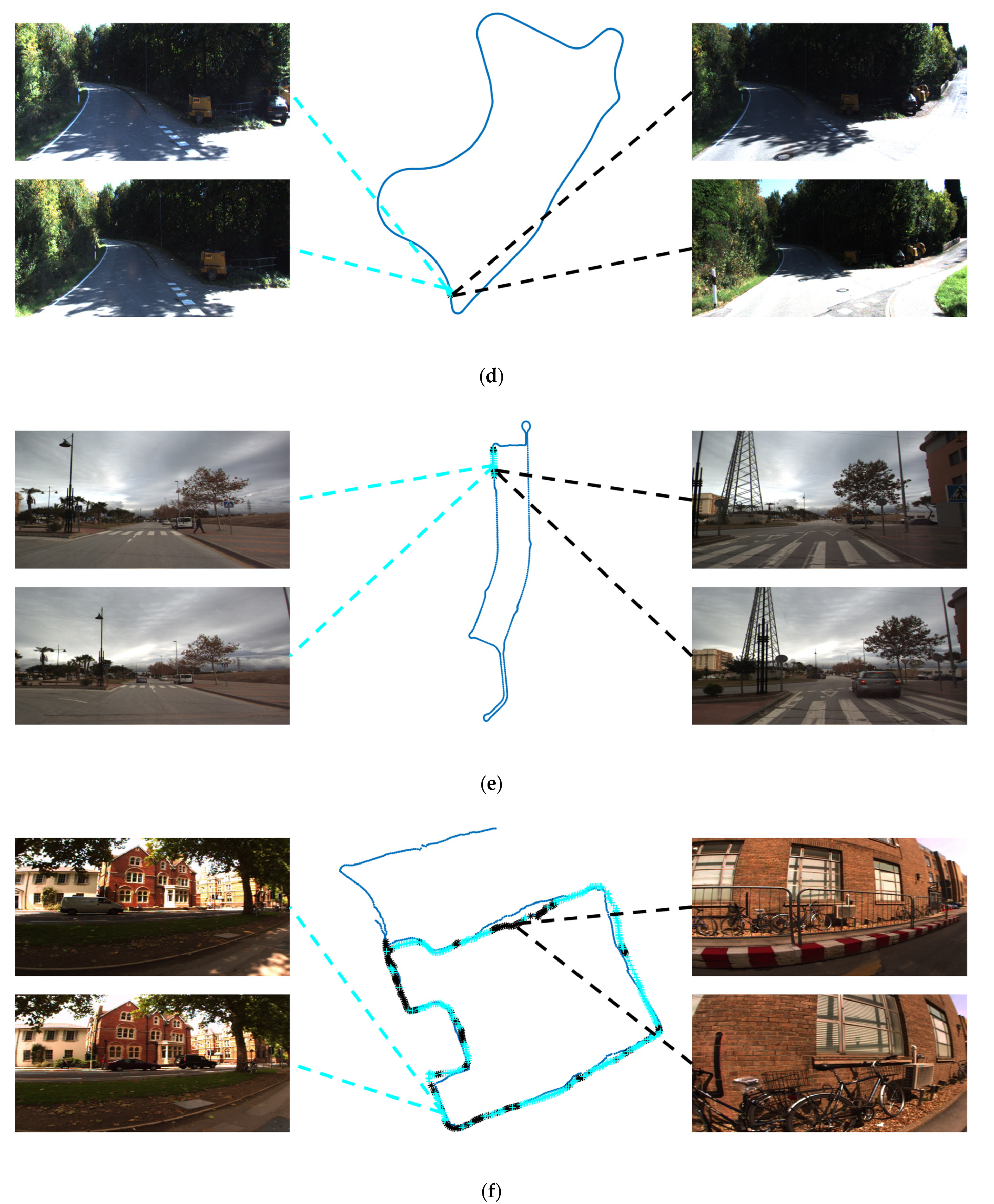
4.1.1. Datasets

To evaluate the performance of our proposed framework, we conduct experiments on six public and challenging sequences, and their details are shown in Table 1. These datasets were collected in different environments, for example, with strong visual repetition and interference from dynamic objects, such as cars and pedestrians. Four of them are KITTI00, KITTI05, KITTI06, and KITTI09 which are representative sequences of the KITTI vision benchmark suite dataset [39]. The author in [25] provided corresponding ground truths. Another image sequence is the Malaga dataset “urban#8” (Malaga#8) in [40], which was taken in an urban road scene with a travel distance of 4.5 km. We manually analyzed the GPS information of the dataset and set the image pairs within 20 m to be true loop closures. To test the performance of the proposed algorithm in weakly textured boundary scenarios, we also performed experiments on the City Centre (CC) dataset. CC is captured by the left and right cameras installed in the vision system of a wheeled robot. Each image is mainly occupied by buildings and therefore contains less boundary texture information. The left images of CC are employed in the evaluation and its ground truth was provided by the authors in [18].

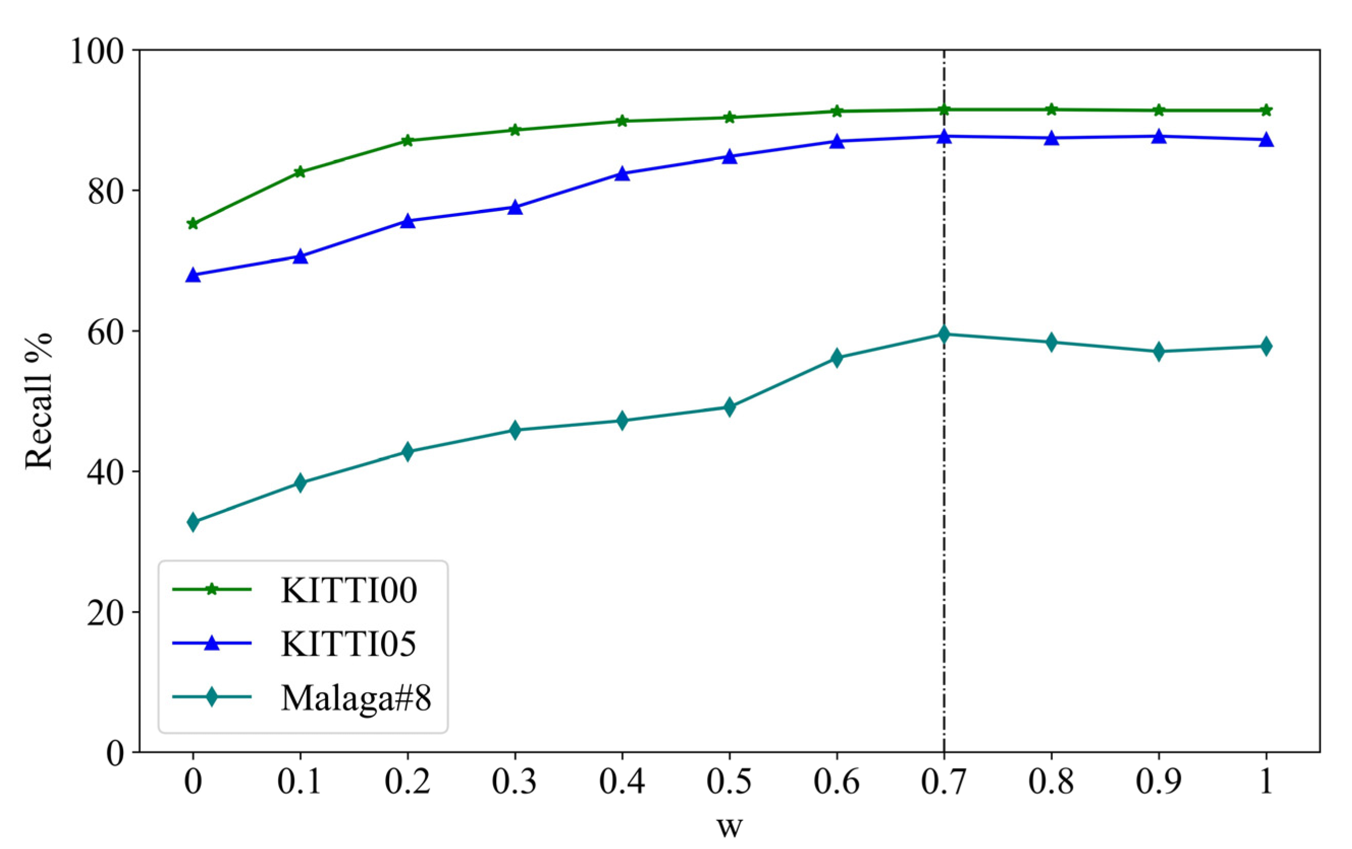
4.1.2. Parameters Setting

We fix the weights of the feature extraction module and train the global feature ranking branch on the KITTI02 sequence using transfer learning. The margins γ for the HPHN quadruplet loss are set to 0.5. The input images are resized to 544 × 544. Adam optimizer is used for training 30 epochs with a learning rate of 1 × 10⁻⁶. We set the batch size to 1 and each batch includes a quadruplet with 2 positive images and 9 negative images (including 1 randomly sampled image). All experiments are conducted on an Intel(R) Core i7-11700F [email protected] computer with a GeForce GTX 3080Ti GPU card.

4.1.3. Evaluation Metrics

We use the recall rate at 100% precision to evaluate our proposed method. The precision and recall can be calculated by Equations (8) and (9). Precision is defined as the number of true positive loops over the total number of loops that the algorithm detected. Recall refers to the ratio between the number of true positive loops and the total number of loops defined in the ground truth.
Precision = True positives True positives + False positives
Recall = True positives True positives + False negatives

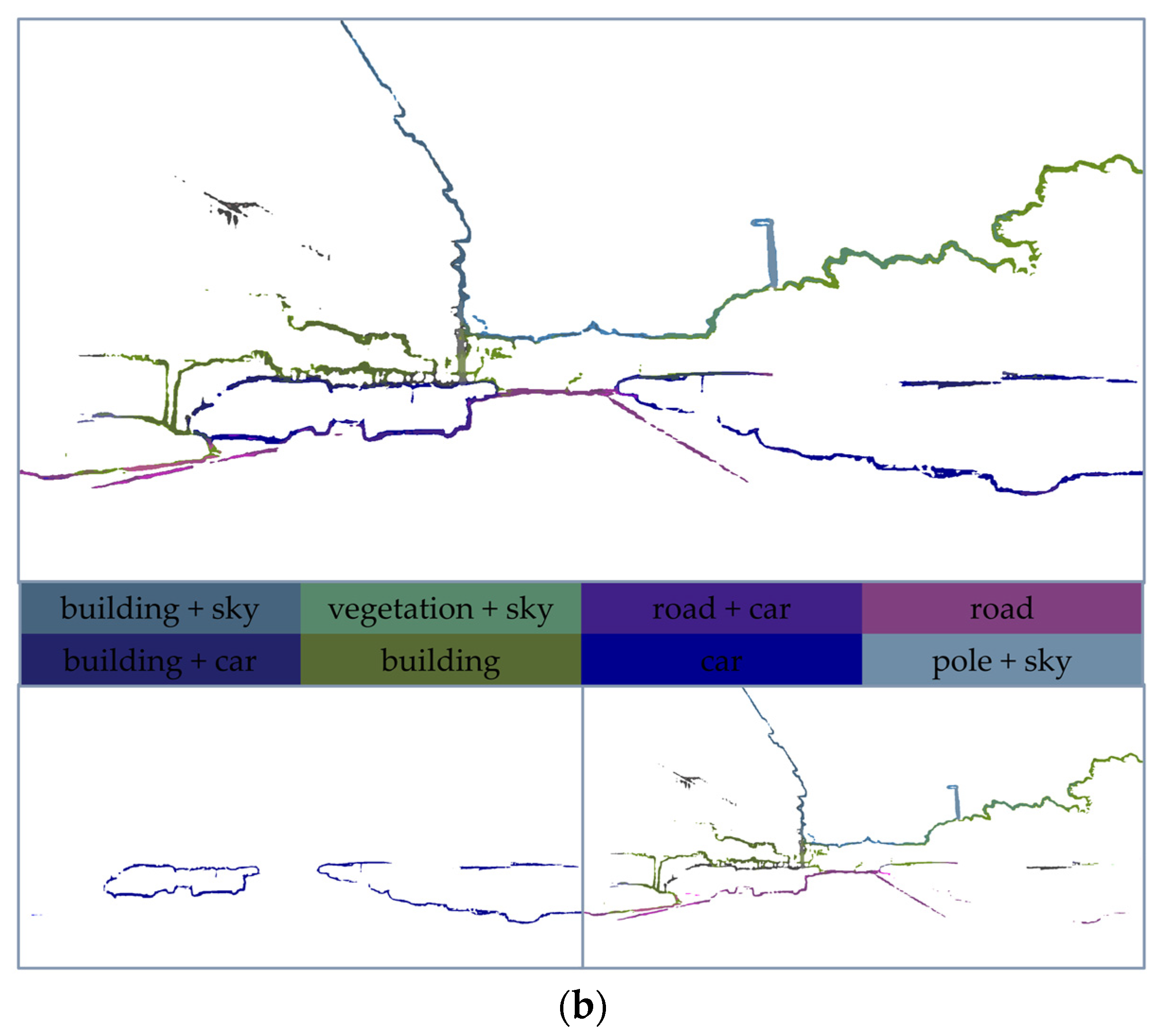
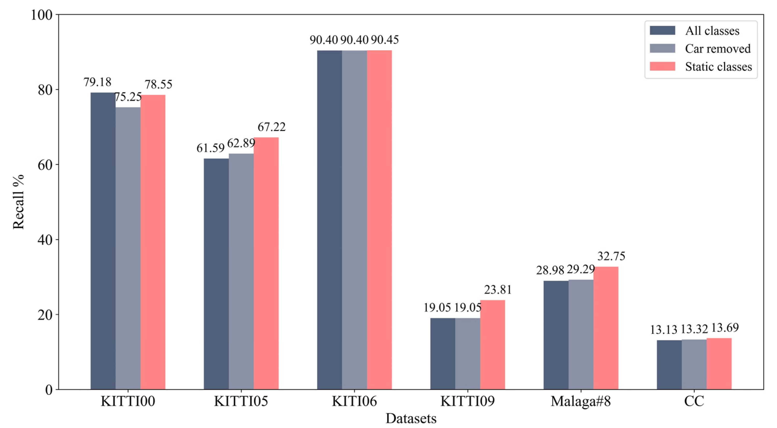
4.2. Effect of Semantic Categories for Semantic Edge Descriptor

To investigate the impact of dynamic semantic edge categories on the semantic feature ranking branch, we test the max recall of different subsets of the 19 semantic edge categories on six datasets. The results are shown in Figure 4, where “All classes” means that the semantic edge descriptor is constructed using 19 semantic classes., “Car removed” means that the semantic edges of the car class are removed when building the semantic edge descriptor, “Static classes” means using only 11 static semantic categories of edges. As shown in Figure 4, five of the six datasets achieved the highest recall using only static classes. In particular, on the KITTI05 dataset, using only static classes improved the recall by 5.63% compared to using all classes. On the KITTI00 dataset, the removal of the semantic edges of the car class caused a decrease in accuracy. This is due to the characteristics of the dataset, where many of the loop closure images contain stationary vehicles parked at the roadside, and the semantic edges of these vehicles are useful for loop closure judgments. In most cases, removing dynamic semantic classes helps to improve the accuracy and reliability of the LCD system. In the following experiments, we use only static classes for the construction of semantic edge descriptors.

4.3. Effectiveness of Context Feature Enhanced (CFE) Module

Table 2 presents the max recall rates at 100% precision of the global feature ranking branch with and without the CFE module on six datasets. According to Table 2, compared to the global feature ranking branch without the CFE module, the recall rates of the algorithm with the CFE module increase by 0.25% (KITTI00) to 6.72% (KITTI06). The results show that the CFE module is capable of learning low-level boundary textures, aggregating context information, and improving the representation ability of global features.

4.4. Effectiveness of Descriptors for Two Branches

To analyze the performance of the two kinds of features, we compare the precision-recall curves for six evaluation sequences by varying the inliner number of two branches. As shown in Figure 5, KITTI06 achieves the highest recall rate in each of the two branches. In Figure 5a, the recall rate of the CC dataset at 100% precision is 68.97%. However, in Figure 5b, the recall rate is 13.69%, which indicates that when there is a lack of sufficient edge information in the loop closure images, the recall of the semantic edge feature ranking branch will perform poorly, and the global feature ranking branch can still work stably. It is noticed that in Figure 5, the performance of the two features varies somewhat across datasets. The convolution features generally outperform the semantic edge features.
In the two-branch fusion calculation, we perform a weighted fusion of the similarities obtained from the global feature ranking branch and the semantic edge feature ranking branch. To take full advantage of the two branches, we investigate the maximum recall of the system with different weight fusion coefficients w on KITTI00, KITTI05, and Malaga#8 datasets. Results in Figure 6 show that as the weight w increases (i.e., the weight of the candidates in the global feature ranking branch increases), the recall of the system tends to increase on the three datasets. Additionally, when w = 0.7, the three datasets obtain the best performance. Based on the experimental results, we set w = 0.7 in our fusion calculation.

4.5. Comparative Results

Figure 7 shows the ground truth trajectory and our loop closure detection results at 100% precision of KITTI 00, KITTI05, KITTI06, KITTI09, Malaga#8, and CC datasets. The blue line indicates the robot trajectory obtained from the ground truth provided by each dataset. The cyan dots indicate the loop closures found by the proposed method and the black dots represent false negative loop closures. In order to intuitively display the prediction results of the model, we randomly select a pair of true loop closures and a pair of false negative loop closures in each dataset and scale them up. We can see that the scenes that correspond to true loop closures in Figure 7 contain small dynamic objects, which indicates that our proposed method is robust for little viewpoint change and small dynamic object inference. The scenes that correspond to false negative loop closures are accompanied by significant changes in perspective or insufficient static feature information, which make loop closure detection difficult even for human eyes. In general, our proposed method can accurately detect most of the true loops even when there are some viewpoint changes or medium dynamic objects.
We compare our method with various state-of-the-art and typical LCD algorithms including: DloopDetector [19], Tsintotas et al. [21], Kazmi et al. [41], FILD [25], BoTW-LCD [22], and SVG-Loop [42]. DloopDetector is the most classic and practical method in LCD. Tsintotas et al. and BoTW-LCD are open-source and influential algorithms based on traditional features. Kazmi et al. and FILD are popular visual LCD methods based on ConvNet features. SVG-Loop is the latest LCD framework based on semantic, visual, and geometric information. Table 3 shows the recall rates at 100% precision of different algorithms on six sequences. ‘-’ indicates that the comparison algorithms are not experimented on the dataset due to hardware limitations or unavailable source code.
As shown in Table 3, our proposed framework outperforms the other approaches in four sequences KITTI05, KITTI06, KITTI09, and Malaga#8, where the performance is improved mainly because the environment contains rich semantic, boundary, and texture information, which are the foundation of the proposed method to generate loop closure candidates. The undetected loop closures in KITTI00 mainly occur at corners with large viewpoint variations (as shown in Figure 7). BoTW-LCD achieves the highest recall on KITTI00 with a low amount of unique visual words generated through feature tracking. Weakly textured boundary scenarios in the CC dataset pose a great challenge to the proposed method which heavily depends on deep ConvNet features and semantic edge features. However, our approach can still achieve a competitive result by unifying these two kinds of features in two branches complementarily.

5. Discussion

5.1. Experiments Analysis

Based on the proposed algorithm and the experiment results, the following points need to be emphasized.
  • In contrast to the LCD algorithm using only semantic edges, the proposed method incorporates abstract convolutional features as well. Furthermore, the experiment results show that the performance of the convolutional features is better than that of the semantic edge features. By fusing the two different features, the system achieves the best performance.
  • In the processing of semantic edge features, we artificially remove the edge feature points of dynamic semantic attributes. Additionally, it is demonstrated in the experimental results that removing dynamic features helps to achieve a higher accuracy rate. However, as edge points often have two or more attributes, the results can still be disturbed by dynamic object boundary points, especially when dynamic objects occupy a certain proportion of the picture.
  • As the test datasets do not contain the ground truth of semantic edges, the feature extraction module has to use the weights pre-trained on the Cityscapes dataset, which damages the accuracy of our learning-based method. Even so, the proposed algorithm achieves competitive results.

5.2. Experiment Implementation and Runtime Analysis

We implemented the proposed algorithm in three steps: (1) feature extraction and global feature ranking. (2) VLAD codebook construction and semantic descriptor generation. (3) fusion calculation. The results are shown in Table 4. For a single image, it takes approximately 0.38s to obtain both semantic and ConvNet features. The semantic ranking branch was trained on CPUs. When integrating into the SLAM system, the algorithm can use the keyframes output by the front-end visual odometer or adjust the sliding step (determining the detection gap) to match the real-time requirement of the SLAM system.

6. Conclusions

In this paper, a novel LCD framework unifying deep ConvNet and semantic edge features with a two-branch structure is proposed. The proposed method takes Multi-ResNet as a feature extraction module to extract two different kinds of features (ConvNet features and semantic edge features), allowing for maximum shared computation. The two-branch structure retrieves loop closure candidates based on abstract ConvNet features and figurative semantic edge features, respectively. Finally, the advantages of the two kinds of features are combined through fusion calculation. Experimental results on six public sequences show the effectiveness of the proposed system compared to other contemporary state-of-the-art algorithms.

Author Contributions

Conceptualization, J.B., Y.X. and J.H.; methodology, J.B., Y.X. and J.H.; software, J.B.; validation, J.J. and J.H.; formal analysis, J.B. and Y.X.; investigation, J.J.; resources, Y.X.; data curation, J.B.; writing—original draft preparation, J.B.; writing—review and editing, J.J. and Y.X.; visualization, J.B. and J.H.; supervision, J.H.; project administration, J.J., J.B. and Y.X.; funding acquisition, J.J and Y.X. All authors have read and agreed to the published version of the manuscript.

Funding

This research was founded by the National Key R&D Program of China (Grant No. 2021YFC2201902) and the Tianjin Transportation Science and Technology Development Plan (Project No. 202234).

Data Availability Statement

The data presented in this study are available in [18,39,40].

Acknowledgments

We would like to sincerely thank Konstantinos A. Tsintotas and Shan An for providing the ground truth for the datasets.

Conflicts of Interest

The authors declare no conflict of interest.

References

  1. Palomeras, N.; Carreras, M.; Andrade-Cetto, J. Active SLAM for Autonomous Underwater Exploration. Remote Sens. 2019, 11, 2827. [Google Scholar] [CrossRef]
  2. Cadena, C.; Carlone, L.; Carrillo, H.; Latif, Y.; Scaramuzza, D.; Neira, J.; Reid, I.; Leonard, J.J. Past, Present, and Future of Simultaneous Localization and Mapping: Toward the Robust-Perception Age. IEEE Trans. Robot. 2016, 32, 1309–1332. [Google Scholar] [CrossRef]
  3. Ho, K.L.; Newman, P. Detecting Loop Closure with Scene Sequences. Int. J. Comput. Vis. 2007, 74, 261–286. [Google Scholar] [CrossRef]
  4. Williams, B.; Klein, G.; Reid, I. Automatic Relocalization and Loop Closing for Real-Time Monocular SLAM. IEEE Trans. Pattern Anal. Mach. Intell. 2011, 33, 1699–1712. [Google Scholar] [CrossRef]
  5. Sivic, J.; Zisserman, A. Video Google: A text retrieval approach to object matching in videos. In Proceedings of the IEEE International Conference on Computer Vision, Nice, France, 13–16 October 2003; pp. 1470–1477. [Google Scholar]
  6. Jegou, H.; Perronnin, F.; Douze, M.; Sanchez, J.; Perez, P.; Schmid, C. Aggregating Local Image Descriptors into Compact Codes. IEEE Trans. Pattern Anal. Mach. Intell. 2012, 34, 1704–1716. [Google Scholar] [CrossRef]
  7. Perronnin, F.; Dance, C. Fisher Kernels on Visual Vocabularies for Image Categorization. In Proceedings of the IEEE Conference on Computer Vision and Pattern Recognition, Minneapolis, MN, USA, 17–22 June 2007; pp. 1–8. [Google Scholar]
  8. Tsintotas, K.A.; Bampis, L.; Gasteratos, A. The Revisiting Problem in Simultaneous Localization and Mapping: A Survey on Visual Loop Closure Detection. IEEE Trans. Intell. Transp. 2022. [Google Scholar] [CrossRef]
  9. Radenovic, F.; Tolias, G.; Chum, O. CNN Image Retrieval Learns from BoW: Unsupervised Fine-Tuning with Hard Examples. In Proceedings of the 14th European Conference on Computer Vision, Amsterdam, The Netherlands, 8–16 October 2016; pp. 3–20. [Google Scholar]
  10. Zhang, X.; Su, Y.; Zhu, X. Loop closure detection for visual SLAM systems using convolutional neural network. In Proceedings of the International Conference on Automation and Computing, Huddersfield, UK, 7–8 September 2017; pp. 1–6. [Google Scholar]
  11. Gawel, A.; Don, C.D.; Siegwart, R.; Nieto, J.; Cadena, C. X-View: Graph-Based Semantic Multi-View Localization. IEEE Robot. Autom. Lett. 2018, 3, 1687–1694. [Google Scholar] [CrossRef]
  12. Benbihi, A.; Aravecchia, S.; Geist, M.; Pradalier, C. Image-Based Place Recognition on Bucolic Environment Across Seasons From Semantic Edge Description. In Proceedings of the IEEE International Conference on Robotics and Automation, Paris, France, 31 May–31 August 2020; pp. 3032–3038. [Google Scholar]
  13. Toft, C.; Olsson, C.; Kahl, F. Long-term 3D Localization and Pose from Semantic Labellings. In Proceedings of the International Conference on Computer Vision Workshops, Venice, Italy, 22–29 October 2017; pp. 650–659. [Google Scholar]
  14. Yu, X.; Chaturvedi, S.; Feng, C.; Taguchi, Y.; Lee, T.; Fernandes, C.; Ramalingam, S. VLASE: Vehicle Localization by Aggregating Semantic Edges. In Proceedings of the IEEE/RSJ International Conference on Intelligent Robots and Systems, Madrid, Spain, 1–5 October 2018; pp. 3196–3203. [Google Scholar]
  15. Lin, S.; Wang, J.; Xu, M.; Zhao, H.; Chen, Z. Topology Aware Object-Level Semantic Mapping Towards More Robust Loop Closure. IEEE Robot. Autom. Lett. 2021, 6, 7041–7048. [Google Scholar] [CrossRef]
  16. Oliva, A.; Torralba, A. Building the gist of a scene: The role of global image features in recognition. Prog. Brain Res. 2006, 155, 23–36. [Google Scholar]
  17. Dalal, N.; Triggs, B. Histograms of oriented gradients for human detection. In Proceedings of the IEEE Computer Society Conference on Computer Vision and Pattern Recognition, San Diego, CA, USA, 20–25 June 2005; pp. 886–893. [Google Scholar]
  18. Cummins, M.; Newman, P. FAB-MAP: Probabilistic localization and mapping in the space of appearance. Int. J. Robot. Res. 2008, 27, 647–665. [Google Scholar] [CrossRef]
  19. Galvez-Lopez, D.; Tardos, J.D. Bags of Binary Words for Fast Place Recognition in Image Sequences. IEEE Trans. Robot. 2012, 28, 1188–1197. [Google Scholar] [CrossRef]
  20. Garcia-Fidalgo, E.; Ortiz, A. Hierarchical Place Recognition for Topological Mapping. IEEE Trans. Robot. 2017, 33, 1061–1074. [Google Scholar] [CrossRef]
  21. Tsintotas, K.A.; Bampis, L.; Gasteratos, A. Assigning Visual Words to Places for Loop Closure Detection. In Proceedings of the IEEE International Conference on Robotics and Automation, Brisbane, QLD, Australia, 21–25 May 2018; pp. 5979–5985. [Google Scholar]
  22. Tsintotas, K.A.; Bampis, L.; Gasteratos, A. Modest-vocabulary loop-closure detection with incremental bag of tracked words. Robot. Auton. Syst. 2021, 141, 103782. [Google Scholar] [CrossRef]
  23. Lategahn, H.; Beck, J.; Kitt, B.; Stiller, C. How to Learn an Illumination Robust Image Feature for Place Recognition. In Proceedings of the IEEE Intelligent Vehicles Symposium, Gold Coast, Australia, 23–26 June 2013; pp. 285–291. [Google Scholar]
  24. Chen, Z.; Lam, O.; Jacobson, A.; Milford, M. Convolutional Neural Network-based Place Recognition. arXiv 2014, arXiv:1411.1509. [Google Scholar]
  25. An, S.; Che, G.; Zhou, F.; Liu, X.; Ma, X.; Chen, Y. Fast and Incremental Loop Closure Detection Using Proximity Graphs. In Proceedings of the IEEE/RSJ International Conference on Intelligent Robots and Systems, Macau, China, 3–8 November 2019; pp. 378–385. [Google Scholar]
  26. Sandler, M.; Howard, A.; Zhu, M.; Zhmoginov, A.; Chen, L. MobileNetV2: Inverted Residuals and Linear Bottlenecks. In Proceedings of the IEEE Conference on Computer Vision and Pattern Recognition, Salt Lake City, UT, USA, 18–23 June 2018; pp. 4510–4520. [Google Scholar]
  27. Arandjelovic, R.; Gronat, P.; Torii, A.; Pajdla, T.; Sivic, J. NetVLAD: CNN Architecture for Weakly Supervised Place Recognition. IEEE Trans. Pattern Anal. Mach. Intell. 2018, 40, 1437–1451. [Google Scholar] [CrossRef]
  28. Yu, J.; Zhu, C.; Zhang, J.; Huang, Q.; Tao, D. Spatial Pyramid-Enhanced NetVLAD With Weighted Triplet Loss for Place Recognition. IEEE Trans. Neural Netw. Learn. 2020, 31, 661–674. [Google Scholar] [CrossRef]
  29. Wang, Z.; Li, J.; Khademi, S.; van Gemert, J. Attention-Aware Age-Agnostic Visual Place Recognition. In Proceedings of the IEEE/CVF International Conference on Computer Vision Workshop, Seoul, Korea, 27–28 October 2019; pp. 1437–1446. [Google Scholar]
  30. Chen, Z.; Liu, L.; Sa, I.; Ge, Z.; Chli, M. Learning Context Flexible Attention Model for Long-Term Visual Place Recognition. IEEE Robot. Autom. Lett. 2018, 3, 4015–4022. [Google Scholar] [CrossRef]
  31. Kim, H.J.; Dunn, E.; Frahm, J. Learned Contextual Feature Reweighting for Image Geo-Localization. In Proceedings of the IEEE Conference on Computer Vision and Pattern Recognition, Honolulu, HI, USA, 21–26 July 2017; pp. 3251–3260. [Google Scholar]
  32. Acuna, D.; Kar, A.; Fidler, S. Devil is in the Edges: Learning Semantic Boundaries from Noisy Annotations. In Proceedings of the IEEE Conference on Computer Vision and Pattern Recognition, Long Beach, CA, USA, 15–20 June 2019; pp. 11067–11075. [Google Scholar]
  33. Wang, Y.; Qiu, Y.; Cheng, P.; Duan, X. Robust Loop Closure Detection Integrating Visual-Spatial-Semantic Information via Topological Graphs and CNN Features. Remote Sens. 2020, 12, 3890. [Google Scholar] [CrossRef]
  34. Cordts, M.; Omran, M.; Ramos, S.; Rehfeld, T.; Enzweiler, M.; Benenson, R.; Franke, U.; Roth, S.; Schiele, B. The Cityscapes Dataset for Semantic Urban Scene Understanding. In Proceedings of the IEEE Conference on Computer Vision and Pattern Recognition, Seattle, WA, USA, 27–30 June 2016; pp. 3213–3223. [Google Scholar]
  35. He, K.; Zhang, X.; Ren, S.; Sun, J. Deep Residual Learning for Image Recognition. In Proceedings of the IEEE Conference on Computer Vision and Pattern Recognition, Las Vegas, NV, USA, 27–30 June 2016; pp. 770–778. [Google Scholar]
  36. Radenovic, F.; Tolias, G.; Chum, O. Fine-Tuning CNN Image Retrieval with No Human Annotation. IEEE Trans. Pattern Anal. Mach. Intell. 2019, 41, 1655–1668. [Google Scholar] [CrossRef]
  37. Zhuang, F.; Qi, Z.; Duan, K.; Xi, D.; Zhu, Y.; Zhu, H.; Xiong, H.; He, Q. A Comprehensive Survey on Transfer Learning. Proc. IEEE. 2021, 109, 43–76. [Google Scholar] [CrossRef]
  38. Xia, Y.; Xu, Y.; Li, S.; Wang, R.; Du, J.; Cremers, D.; Stilla, U. SOE-Net: A Self-Attention and Orientation Encoding Network for Point Cloud based Place Recognition. In Proceedings of the IEEE/CVF Conference on Computer Vision and Pattern Recognition, Nashville, TN, USA, 20–25 June 2021; pp. 11343–11352. [Google Scholar]
  39. Geiger, A.; Lenz, P.; Urtasun, R. Are we ready for autonomous driving? The KITTI vision benchmark suite. In Proceedings of the IEEE Conference on Computer Vision and Pattern Recognition, Providence, RI, USA, 16–21 June 2012; pp. 3354–3361. [Google Scholar]
  40. Blanco-Claraco, J.; Moreno-Duenas, F.; Gonzalez-Jimenez, J. The Malaga urban dataset: High-rate stereo and LiDAR in a realistic urban scenario. Int. J. Robot. Res. 2014, 33, 207–214. [Google Scholar] [CrossRef]
  41. Kazmi, S.M.A.M.; Mertsching, B. Detecting the Expectancy of a Place Using Nearby Context for Appearance-Based Mapping. IEEE Trans. Robot. 2019, 35, 1352–1366. [Google Scholar] [CrossRef]
  42. Yuan, Z.; Xu, K.; Zhou, X.; Deng, B.; Ma, Y. SVG-Loop: Semantic-Visual-Geometric Information-Based Loop Closure Detection. Remote Sens. 2021, 13, 3520. [Google Scholar] [CrossRef]
Figure 1. An overview of the proposed module. As the incoming image stream enters the pipeline, the ConvNet features and the semantic edge features of the image are extracted by the feature extraction module. The first ones enter the global feature ranking branch to retrieve the most similar ConvNet candidates. The semantic edges are sent to the semantic edge feature ranking branch to select the most similar images in human vision. Finally, the matched image pair is generated by similarity score fusion computation.
Remotesensing 14 04885 g001
Figure 2. The overall architecture of our proposed Context Feature Enhanced (CFE) module.
Remotesensing 14 04885 g002
Figure 3. Visualization of semantic edge features. (a) raw image. (b) semantic edge images of all categories (above), dynamic categories (bottom left) and static categories (bottom right).
Remotesensing 14 04885 g003aRemotesensing 14 04885 g003b
Figure 4. Effect of semantic categories on six datasets.
Remotesensing 14 04885 g004
Figure 5. The Precision-Recall curves of the two branches on six datasets. (a) Global feature ranking branch. (b) Semantic edge feature ranking branch.
Remotesensing 14 04885 g005
Figure 6. Effect of weighted fusion on KITTI00, KITTI05, Malaga#8 datasets.
Remotesensing 14 04885 g006
Figure 7. Trajectories of the six datasets and all detected loop closures and false negative loop closures at 100% precision. (a) Results of the proposed method on KITTI00. (b) Results of the proposed method on KITTI05. (c) Results of the proposed method on KITTI06. (d) Results of the proposed method on KITTI09. (e) Results of the proposed method on Malaga#8. (f) Results of the proposed method on CC.
Remotesensing 14 04885 g007aRemotesensing 14 04885 g007b
Table 1. Descriptions of the used datasets.
DatasetDescriptionImage Resolution#ImagesFrame Rate (Hz)Distance (km)
KITTISeq#00Outdoor dynamic1241 × 3764541103.7
Seq#021241 × 37646615.0
Seq#051226 × 37027612.2
Seq#061226 × 37011011.2
Seq#091221 × 37015911.7
Malaga datasetUrban#8Outdoor slightly dynamic1024 × 76810026204.5
OxfordCity CenterOutdoor dynamic640 × 4801237101.9
Table 2. The comparative results of the global feature ranking branch with and without the CFE module on six datasets.
DatasetsWithout CFE ModuleWith CFE Module
Precision (%)Recall (%)Precision (%)Recall (%)
KITTI0010091.1210091.37
KITTI0510085.0610087.22
KITTI0610090.4110097.03
KITTI0910090.4810095.23
Malaga#810057.0310057.80
CC10062.6810068.97
Table 3. Recall rates at 100% precision of different algorithms.
ApproachKITTI00KITTI05KITTI06KITTI09Malaga#8CC
DloopDetector [19]78.4267.5990.4441.8717.8030.59
Tsintotas et al. [21]76.5053.0795.5387.8926.8082.03
Kazmi et al. [41]90.3981.4197.39--75.58
FILD [25]91.2365.1193.38--66.48
BoTW-LCD [22]93.7883.1394.4690.4841.3736.00
SVG-Loop [42]73.5147.8758.1150.46--
Proposed91.5087.4697.7895.2359.5368.61
Table 4. Average processing time of per image in KITTI00, Malaga#8 and CC sequences.
Average Time (s)
KITTI00Malage#8CC
Feature extraction0.38780.39010.3817
Global feature ranking
Semantic descriptor generation0.44580.40040.4029
Fusion calculation0.00410.01090.0006
Total0.83770.80140.7852
Publisher’s Note: MDPI stays neutral with regard to jurisdictional claims in published maps and institutional affiliations.

