Abstract
Owing to the limitation of spatial resolution and spectral resolution, deep learning methods are rarely used for the classification of multispectral remote sensing images based on the real spectral dataset from multispectral remote sensing images. This study explores the application of a deep learning model to the spectral classification of multispectral remote sensing images. To address the problem of the large workload with respect to selecting training samples during classification by deep learning, first, linear spectral mixture analysis and the spectral index method were applied to extract the pixels of impervious surfaces, soil, vegetation, and water. Second, through the Euclidean distance threshold method, a spectral dataset of multispectral image pixels was established. Third, a deep learning classification model, ResNet-18, was constructed to classify Landsat 8 OLI images based on pixels’ real spectral information. According to the accuracy assessment, the results show that the overall accuracy of the classification results can reach 0.9436, and the kappa coefficient can reach 0.8808. This study proposes a method that allows for the more optimized establishment of the actual spectral dataset of ground objects, addresses the limitations of difficult sample selection in deep learning classification and of spectral similarity in traditional classification methods, and applies the deep learning method to the classification of multispectral remote sensing images based on a real spectral dataset.
1. Introduction
Ground objects are the main targets of remote sensing detection, and different spectral reflectance curves can reflect the characteristics of the corresponding pixels [1]. Using the computer to analyze the spectral information and spatial information of various ground objects in the remote sensing image, the corresponding features are selected, each pixel in the image is divided into different categories according to a certain rule or algorithm, and then the difference between the remote sensing image and the actual ground is determined. The corresponding information on objects can be used to classify images or extract target objects [2].
Remote sensing images have two important attributes: spatial resolution and spectral resolution. The spatial resolution of multispectral remote sensing images is generally higher than that of hyperspectral remote sensing images, and the spectral resolution of multispectral remote sensing images is generally higher than that of high-spatial-resolution remote sensing images [3]. In addition, multispectral remote sensing image series, especially the Landsat series, provide long-term remote sensing images; the data are relatively easy to obtain, and the theoretical basis of data preprocessing is solid. Therefore, the remote sensing images of this series are often used as data sources for long-term series analysis and research.
In multispectral remote sensing image classification research, spectral index and spectral unmixing methods are commonly used as classification methods. They are based on pixel and sub-pixel scales, respectively, and allow for the identification and classification of target objects according to their spectral characteristics [4,5]. The spectral index method uses the spectral characteristics of objects in remote sensing images in different bands to reflect the spatiotemporal distribution of specific target objects [6]. The normalized difference vegetation index (NDVI) [7] is a common spectral index for identifying vegetation. It quantifies vegetation according to the obvious differences in the spectral characteristics of vegetation in the near-infrared and red bands. The greater the vegetation coverage in a mixed pixel, the larger the NDVI value of the pixel. Similar to the theoretical basis of NDVI for identifying vegetation, the Dry Bare Soil Index (DBSI) [8] and the Ratio of Normalized Difference Soil Index (RNDISI) [9,10] exhibit more optimized performance in soil identification. The normalized impervious surface index (NDISI) [11,12], normalized building index (NDBI) [13], normalized differential impervious surface index (NDII) [14], biophysical component index (BCI) [15], and urban index (UI) [16] can enhance IS pixels in remote sensing images. The modified normalized difference water index (MNDWI) enhances the characteristics of water pixels and distinguishes between ISs from water [17]. The spectral unmixing method involves the use of the spectral characteristics of mixed pixels and pure pixels to calculate the area ratio (fraction) of various objects in mixed pixels [18,19]. The vegetation-impervious surface-soil (V-I-S) model [20] was proposed in 1995. The model simplifies the urban surface cover type with strong heterogeneity into a combination of different fractions of vegetation, IS, and soil in the case of water pixels [21]. IS pixels are generally divided into two categories: high-reflectivity ISs (e.g., white roofs and white buildings) and low-reflectivity ISs (e.g., asphalt roads) [22,23]. A linear spectral mixture analysis (LSMA) assumes that the reflectance of each mixed pixel in a certain wavelength band is a linear combination of the reflectance of each component in the pixel in the same wavelength band [24,25,26], and it assumes that the coefficient of each reflectance is determined by the area ratio of the component in the pixel [27]. Combining the spectral index method and the spectral unmixing method plays an important role in optimizing the spectral unmixing results [28,29], as the calculation of the correlation index improves the accuracy of pure-pixel selection for LSMA. The above studies show that the spectral index method and the spectral unmixing method have a suitable theoretical basis and practical value for the identification of ground objects based on spectra.
In recent years, deep learning has yielded remarkable scientific results in many fields. In research on the classification of remote sensing images, deep learning comprehensively considers the spatial and spectral characteristics of target objects. This method is usually used for image classification and target object extraction for remote sensing images with high spectral and spatial resolutions. Deep learning models autonomously learn features from data and do not require researchers to pre-design features. They then extract features from data according to pre-designed feature extraction rules. Deep learning network models, including convolutional neural networks [30], deep belief networks [31], and stacked autoencoder networks [32], have also been gradually introduced into the field of remote sensing image classification, particularly in the classification of hyperspectral remote sensing images [33]. Recently, a Hybrid Feature Enhancement Network was proposed to solve the problems that similar features are confusable and small-scale features are difficult to identify in the classification of remote sensing images [34]. In addition, tests on public datasets showed that the combined convolutional neural network (DUA-Net) achieved high accuracy in complex urban land-use classification [35]. The atrous spatial pyramid pooling (ASPP) framework (RAANet: Residual ASPP with Attention Net) enhanced the classification accuracy of semantic segmentation [36]. A seven-layer CNN model greatly improved the classification accuracy, while the best overall accuracy (OA) and Kappa coefficient were 94.68% and 0.9351, respectively [37]. For remote sensing images with medium spatial resolution, some scholars have also tried to apply deep learning; for example, Karra K et al. pointed out that the resolution of global LULC products is currently low, so they used deep learning technology to generate global LULC products with a spatial resolution of 10 m [38]. Other scholars have also tried to classify Landsat images with 15 m and 30 m resolution based on deep learning methods [39,40,41].
In research on classifying remote sensing images based on spectral information, the samples used in remote sensing classification by deep learning are obtained from two sources. One source of sample data is produced by researchers for training and testing in the study area, and the sample production is labor- and time-consuming. The other source is existing public datasets. Actual remote sensing images and public datasets have certain variations, and the datasets cannot be accurately matched with actual remote sensing images. When using the spectral information of ground objects for classification, commonly used spectral libraries include the ECOSTRESS spectral library [42], USGS Digital Spectral Library [43], ASTER Spectral Library [44], ASU Thermal Emission Spectroscopy Laboratory Spectral Library [45], Caltech Mineral Spectroscopy Server [46], CRISM Spectral Library [47], Janice Bishop’s Spectral Library @ SETI [48], Johns Hopkins University Spectral Library [49], USGS View_SPECPR—Software for Plotting Spectra (Version 1.2) [50], etc. However, due to various changes and environmental influences, the spectral characteristics of the above spectral datasets are different from those in the actual images; it is common that pixels containing the same ground objects have different spectral features, and pixels containing different ground objects have the same spectral features. Furthermore, the deep learning model needs to establish a large number of training samples before classification [33], and the spatial characteristics of multispectral remote sensing images are significantly inferior to those of high-spatial-resolution remote sensing images. In addition, their spectral characteristics are inferior to those of hyperspectral remote sensing images, thus complicating the training sample selection to a certain extent.
Spectral index and spectral unmixing methods are commonly used methods for classifying multispectral remote sensing images. However, the use of the spectral index to classify ground objects necessitates the determination of a specific threshold. Furthermore, the spectral unmixing method is often attributed to the selection error of pure pixels and the phenomenon of the “same thing different spectrum” and “foreign matter same spectrum”, resulting in large errors. This often necessitates the culling of water pixels because the spectral reflectance of the water pixels is close to that of the low-albedo impervious surface (IS) (ISs are divided into high-albedo ISs and low-albedo ISs) [4,22].
In this study, the MNDWI was used for the removal of water pixels to calculate LSMA. Then, the spectral information of the pure pixels selected from a Sentinel 2A image was improved by improving the spectral information of the pure pixels selected from a Landsat 8 image. Based on the improved spectral information, LSMA was used to calculate the fraction of vegetation, soil, high IS, and low IS. Meanwhile, MNDWI images were used to extract water pixels [51]. Through the threshold extraction method for the vegetation fraction (VS), soil fraction (SF), IS fraction (ISF), and MNDWI, a real spectral dataset of ground objects for deep learning was established to ease the workload of training sample selection. The ResNet-18 model was applied for Landsat 8 OLI image classification to address the inability of LSMA to distinguish the classifications of ground objects from similar spectral features and alleviate the strong subjectivity when using the spectral index threshold method to classify ground objects. New ideas and a theoretical basis for the classification of ground objects in multispectral remote sensing images are provided.
2. Materials and Methods
2.1. Data
2.1.1. Study Area
The study area comprises the six main urban areas (113°8′E~113°37′E, 23°26′N~23°2′N) of Guangzhou City, Guangdong Province: Yuexiu District, Haizhu District, Tianhe District, Baiyun District, Huangpu District, and Liwan District. The study area location is shown in Figure 1. The main urban area contains typical vegetation, water, bare soil, and urban ISs (roads, buildings, and residential and commercial lands with different densities). Furthermore, in the study area, there are large forest areas with more pure pixels of vegetation in Baiyun District and Huangpu District. At the same time, Baiyun District also contains a large amount of farmland, with more pure pixels of soil. Tianhe District and Yuexiu District have large built-up areas with more pure pixels of impervious surfaces. Therefore, pure pixels are easier to obtain, which is conducive to the extraction of the spectral features of different pixels.
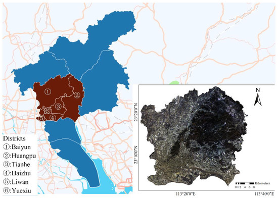
Figure 1.
Study area.
2.1.2. Remote Sensing Data
In this study, the Landsat 8 OLI multispectral remote sensing image acquired on 23 October 2017 was selected as the main research data for classification. The Sentinel 2A MSI multispectral remote sensing image acquired on 1 November 2017 was used as auxiliary research data, and the WorldView-2 high-spatial-resolution image acquired on 20 December 2017 was used as the verification data for the results of LSMA.
The Landsat 8 satellite was launched in February of 2013, and its sensors comprise the OLI and Thermal Infrared Sensor (TIR) [8]. Landsat 8 OLI has 9 reflective wavelength bands, including seven 30 m visible, NIR, and SWIR bands and a 15 m pan band. In this study, we used the seven bands (B1–B7) of Landsat 8 OLI (Path 122/Row 44) (Table 1). The digital numbers of the OLI images were converted to surface reflectance through radiometric calibration and atmospheric correction, which were provided by the United States Geological Survey (USGS) Earth Resources Observation and Science (EROS) Center Science Processing Architecture (ESPA) on-demand interface [52].

Table 1.
Landsat 8 Operational Land Imager (OLI) and Sentinel-2A Multispectral Instrument (MSI) bands.
The Sentinel-2A satellite was launched in June of 2015 and carries the MSI. Sentinel-2A MSI data have thirteen reflective wavelength bands, including four 10 m visible and NIR bands, six 20 m red-edge, near-infrared, and SWIR bands, and three 60 m bands. In this study, we used the blue (B2), green (B3), red (B4), NIR (B8), and SWIR (B11 and B12) bands of the Sentinel-2A MSI data (Table 1). For data preprocessing, atmospheric correction was applied using the onboard Sen2cor processor. Additionally, using the nearest-neighbor method, the spatial resolutions of B11 and B12 were resampled to 10 m by the Sentinel Application Platform (SNAP), the integrated application platform of the Sentinel Series satellite products of the European Space Agency (ESA).
In order to verify the reliability of LSMA, 172 rectangular sample areas were randomly selected in the study area for vectorization to extract vegetation, soil, and impervious surface in the sample area, and then the area ratio of each component in each sample area was calculated as the reference data.
2.2. Methods
As the spatial resolution of Sentinel-2A multispectral remote sensing images exceeds that of Landsat 8 OLI multispectral remote sensing images, the selection of pure pixels from Sentinel 2A MSI is easier. Therefore, the spectral information of pure pixels in Sentinel 2A MSI was used to improve the spectral information of pure pixels in Landsat 8 OLI. Then, LSMA was used to calculate the area ratio of vegetation, soil, and IS in each pixel to obtain the images of the vegetation fraction (VF), soil fraction (SF), and impervious surface fraction (ISF). Meanwhile, the OTSU threshold method was used to process MNDWI images to distinguish water pixels. Then, based on the above classification results, the spectral reflectance values of the pixels in all bands of Landsat 8 OLI images corresponding to each type of ground object were obtained and then extracted using the threshold method and filtered via the Euclidean distance method. The filtered pixel spectral reflectance values were used as a dataset to establish deep learning samples (training samples and verification samples). Finally, a deep learning network model was built for the real spectral characteristics of ground objects to classify Landsat 8 OLI multispectral remote sensing images, which are divided into four categories: vegetation, bare soil, IS, and water. The general research framework is shown in Figure 2.
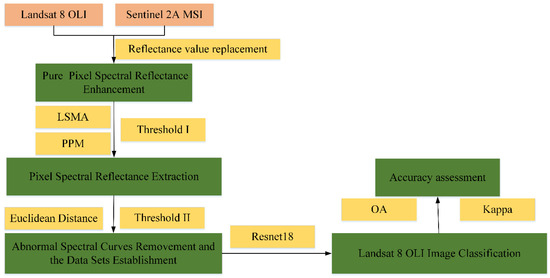
Figure 2.
Research Framework.
2.2.1. Pixel Spectral Reflectance Enhancement and Extraction
Vegetation, Soil, and Impervious Surfaces
- Pure-Pixel Spectral Reflectance Enhancement
Landsat 8 OLI and Sentinel 2A MSI multispectral remote sensing images were preprocessed. Processing included image cropping and layer stacking. In addition, for Sentinel 2A MSI, the spatial resolution in all bands was resampled to 10 m, and the format of the image was unified to TIFF. Water pixels in the Landsat 8 OLI and Sentinel 2 A MSI images were removed according to the threshold for MNDWI images. The MNDWI threshold segmentation method was OTSU [53].
In this study, Sentinel 2A MSI with a higher spatial resolution (10 m) was used to select pixels with relatively high purity and extract the spectral reflectance of these pixels. As shown in the band range presented in Table 1, the spectral reflectance of the “pure pixel” selected from Landsat 8 OLI was replaced with the spectral reflectance of the “pure pixel” selected from Sentinel 2A MSI, and the spectrum closer to the actual ground object pixel was obtained. The curve provides a reliable data basis for the calculation of mixed spectral unmixing, thereby improving the extraction accuracy of spectral unmixing. The specific data processing steps are shown in Figure 3.

Figure 3.
Flow chart for pixel spectral reflectance enhancement.
- 2.
- Pixel Spectral Reflectance Extraction
The improved LSMA with the post-processing model (PPM) and the spectral index threshold method were used to extract the spectral reflectance of ground object pixels in the multispectral remote sensing image. For targets in the image, the vegetation, bare soil, and impervious surface pixels were extracted by LSMA, and water pixels were extracted by the MNDWI threshold. The improved LSMA calculation formula is as follows:
where i = 1, 2…, M, with M denoting the band number; k = 1, 2, …; n is an index of endmembers, with n representing the number of endmembers; Ri is the spectral reflectance of band i within a mixed pixel; f is the fraction of the endmember k; and ERi is the residual error of band i.
The PPM optimized the fractions of various endmembers in the pixels calculated by LSMA. Based on the calculation results of LSMA and the spectral index, including NDVI and DBSI, the PPM adjusted the category attributes of certain pixels and assigned the fraction of the corresponding pixels to the corresponding categories, and the calculation shown in Figure 4 was performed. The calculation formula is as follows:
where is the SF of pixels extracted by LSMA; and are the low-albedo impervious surface fraction (LSIF) and high-albedo impervious surface fraction (HSIF) of pixels extracted by LSMA, respectively; and , and are the final VF, ISF, and SF, respectively.
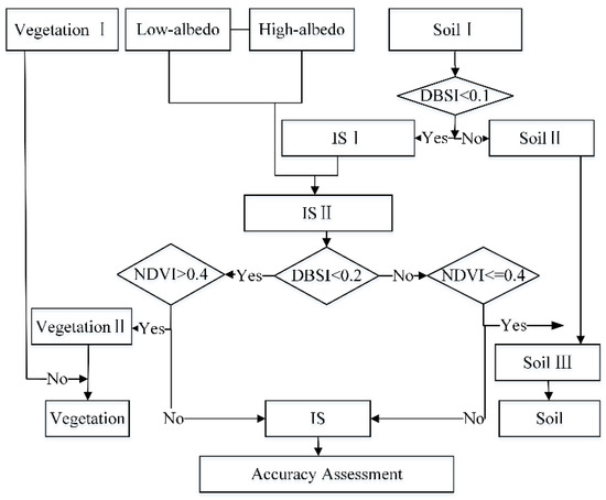
Figure 4.
Flow chart for post-processing model.
Based on the above results, using the threshold method, pixels with ISF exceeding Threshold I (0.75, 0.85) were selected as the IS target pixels, pixels with VF exceeding 0.75 (or 0.85) were selected as the vegetation target pixels to extract vegetation, and pixels with SF exceeding 0.75 (or 0.85) were selected as the soil target pixels. The reflectance of the pixels in the 7 bands of Landsat 8 OLI corresponding to each class was extracted to build datasets including training and test samples for deep learning models, such as vegetation, soil, and IS samples.
Water-Pixel Spectral Reflectance Extraction
The spectral index MNDWI was used as the basis for the spectral characteristics of water pixels. The OTSU threshold method was used to segment the MNDWI. The MNDWI image was divided into two parts: water pixels and non-water pixels. The reflectance of water pixels in the 7 bands of Landsat 8 OLI were extracted to build datasets including training and test samples for deep learning models, such as the water sample.
The calculation formula of the MNDWI is as follows:
where is the reflectance in the green band of the multispectral image, corresponding to B3 and B3 of Landsat 8 OLI and Sentinel 2A MSI, respectively; is the spectral reflectance of the mid-infrared band, corresponding to B6 and B11 of Landsat 8 OLI and Sentinel 2A MSI, respectively.
2.2.2. Accuracy Assessment
According to the LSMA results, the accuracy of ISF and VF was verified. A total of 171 samples with a spatial resolution of 480 m × 480 m were selected randomly. The IS fraction and vegetation fraction of each sample were calculated by dividing the IS area by the total sample area (230,400 m2). The root-mean-square error (RMSE) was computed to test for accuracy using the following formula:
where is the calculation result of LSMA from Landsat 8 OLI, and is the fraction of the validation sample from the WorldView-2 image.
2.2.3. Abnormal Spectral Curve Removal and Dataset Establishment
Abnormal Spectral Curve Removal by Euclidean Distance
To verify the influence of the purity of the spectral information obtained by the above classification methods on the deep learning classification results, the Euclidean distance threshold method was used to screen spectral data. For vegetation, soil, and IS, the spectrum of the pure endmember pixel was regarded as the reference value. For water, the mean reflectance in each band of water pixels was regarded as the reference. After statistical analysis using the threshold method, spectral information with a large Euclidean distance in each class was removed to draw the datasets acting on deep learning closer to the pure spectrum of the real objects. The Euclidean distance calculation formula is as follows:
where is the Euclidean distance of the reflectance curve vectors of two pixels ( and ), is the band, = 7, and and are the spectral reflectance of pixels x and y in band , respectively.
Dataset Establishment
For IS, soil, and vegetation pixels, based on the above classification, this study set 0.75 and 0.85 as the thresholds of the area fraction (Threshold I): pixels with VF exceeding 0.75 (or 0.85) were considered vegetation pixels, pixels with SF exceeding 0.75 (or 0.85) were considered soil pixels, and pixels with ISF exceeding 0.75 (or 0.85) were considered impervious surface pixels. For water pixels, OTSU was applied for MNDWI images.
Subsequently, based on the geographic location of the pixels of various ground objects, the spectral reflectance of the corresponding pixels in the multispectral image in each band was extracted, and the spectral characteristic curve dataset of various ground objects, which is used as the basic sample library for deep learning, was generated. In the basic sample library, for a specific object, the corresponding Euclidean distance was calculated. The smaller the Euclidean distance, the closer the pixel is to the pure pixel, and the more obvious the spectral characteristics of the object. In this study, the Euclidean distance threshold (Threshold II) of the spectral curve of various ground objects was used to optimize the spectral database.
Each type of spectral characteristic curve data was divided into a non-training and training test set, and the distribution ratio was 7:3. Then, the training test set was divided into the training and test set, and the distribution ratio was 3:1, as shown in Figure 5.
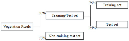
Figure 5.
Schematic of dataset allocation (vegetation).
To explore the influence of the actual pixel spectrum on the classification, this study regarded the high-albedo impervious surface (High IS) and the low-albedo impervious surface (Low IS) as different classes during the Euclidean distance calculation.
The experiments were divided into four categories, as shown in Table 2.
Table 2.
Thresholds for experiments.
Experiment 1 and Experiment 3 mean that the dataset was optimized without using the Euclidean distance threshold.
2.2.4. Deep Learning Model Establishment
When ResNet-18 was initially presented, the model was used for picture recognition [54]. Since then, it has been widely used in remote sensing image semantic segmentation and change detection. Both areas are similarly complicated 2D planar remote sensing imaging tasks in general; however, this research only pertains to spectral curve regression fitting, which is comparatively straightforward compared to 2D planar remote sensing photos. The phenomenon of the “same thing different spectrum” and “foreign matter same spectrum” occurs due to the minor variation in the spectral curves between distinct features, making it difficult for deep learning networks to fit the parameters and making them prone to misfitting. The residual block structure in the ResNet-18 network may enhance the depth of the model network and allow the model to learn deeper characteristics of the spectral curves while avoiding the difficulties of model instability and accuracy loss caused by increasing the depth of the network.
In reference to the ResNet-18 model [55], a deep learning model for classification was built, as shown in Figure 6. The entire model comprises five convolutional structures, a fully connected layer, and an activation function (Softmax) layer.
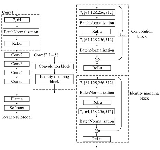
Figure 6.
Deep Learning Model.
The first convolutional structure consists of a 1D convolutional layer, batch normalization layer, and activation layer. The detailed parameters of this layer are as follows: the number of convolution kernels in the 1D convolution layer was 64, the size of the convolution kernel was 7, the padding mode was the same, and the activation function of the activation layer used was Relu. The second to fifth convolution structures had the same form: they consisted of a convolution block and a feature map block, but the number of convolution kernels varied according to the block. The numbers of convolution kernels of the second to fifth convolution structures were 64, 128, 256, and 512, respectively.
There were eight layers in each convolution block: the 1D convolution layer, batch normalization layer, activation layer, 1D convolution layer, batch normalization layer, one-bit short-circuit connection layer, feature fusion layer, and activation layer. The parameters of the block were as follows: Relu was used as the activation function of the activation layer, the convolution kernel size of the 1D convolution layer was set to 3, and the padding mode was the same. The 1D short-circuit connection layer played the role of data dimensionality reduction. The feature map block and the convolution block had the same structure but differed in the sense that the 1D short-circuit connection layer was changed to a feature map layer.
2.2.5. Accuracy Verification Parameters
The Kappa coefficient and overall accuracy (OA) were selected for accuracy verification. The formula is as follows:
where is the total number of samples, is the number of sample categories, is the number of correctly classified samples in each category, and is the number of samples of the classification results for each category.
3. Results
3.1. Results of Vegetation, Soil, and Impervious Surface Extraction
The spectral reflectance of pure pixels obtained from Sentinel 2A MSI was used to optimize the spectral reflectance of pure pixels obtained in Landsat 8 OLI images, and the spectral characteristic curve shown in Figure 7 was obtained. Based on this spectral information, the spectral unmixing results (VF/SF/ISF) of Landsat 8 OLI multispectral remote sensing images are shown in Figure 8. After the accuracy verification of 171 sample areas, the RMSE of ISF was 0.94, and the RMSE of VF was 0.91. The extraction results were highly accurate and can meet the requirements of sample library establishment.
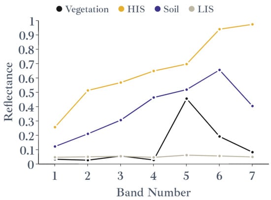
Figure 7.
Result of endmember selection (Threshold I: 0.75).

Figure 8.
Result of LSMA and pixels for Landsat 8 OLI: (a1) impervious surface fractions; (b1) vegetation fractions; (c1) soil fraction; (a2) impervious surface pixels; (b2) vegetation pixels; (c2) soil pixels.
The extraction of various ground object pixels from multispectral images was based on the geographic location. The multispectral image extraction results of IS, soil, and vegetation pixels are shown in Figure 8 with B4, B3 and B2 of Landsat 8 OLI.
3.2. Results of Water Extraction
MNDWI images were used to extract the water pixels in the Landsat 8 OLI multispectral image with the OTSU threshold segmentation method. The MNDWI threshold segmentation result is shown in Figure 9(a1). Furthermore, the results of the multispectral image extraction of water pixels are shown in Figure 9(a2).
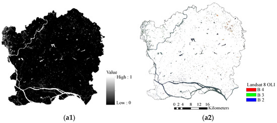
Figure 9.
Water images: (a1) MNDWI segmented by OTSU; (a2) water extraction from Landsat 8 OLI.
3.3. Results of Classification
Figure 10 shows the classification results of Experiments 1 to 4. The resulting image contains four types of objects: IS, soil, vegetation, and water. A large area of vegetation and IS was observed in the study area, and water areas (rivers, lakes, etc.) were more conspicuous. However, the soil was less abundant and sparsely distributed in the northeastern part of the study area. Certain differences were observed in the classification results of the four experiments. In Experiment 1, some water pixels were mistaken as IS pixels. Experiments 2 and 3 also had such problems. Experiment 4 had the best classification results, and the distribution of various ground objects was close to the actual situation.
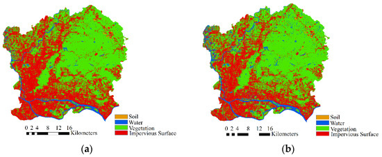
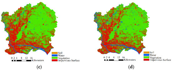
Figure 10.
Classification results by ResNet-18: (a) Experiment 1, (b) Experiment 2, (c) Experiment 3, and (d) Experiment 4.
The overall accuracy of the classification exceeded 0.87, and the overall accuracy of the fourth experiment reached 0.9436. Combined with Figure 10, the classification results of the experiment were relatively reliable.
4. Discussion
Based on multispectral remote sensing images, LSMA and spectral index (MNDWI) methods were used to extract the pixel spectral reflectance of IS, soil, vegetation, and water. This was integrated with the threshold and Euclidean distance methods to establish a dataset for deep learning classification. The ResNet-18 model was developed, and four experiments were used to confirm the feasibility of applying deep learning methods to multispectral remote sensing image classification and to solve the problems of a large sample size and low spatial resolution. The experiment showed that the choice of the threshold can significantly influence the classification results when establishing the real objects’ spectral database.
The improved LSMA was used to extract the pixels of IS, soil, and vegetation from the multispectral remote sensing image (Landsat 8 OLI). Combined with the results of spectral unmixing, the corresponding ground object pixels were extracted using Threshold I, and the spectral reflectance in seven bands was obtained. Spectral index and OTSU threshold segmentation was used to extract pixels of water, and the spectral reflectance pixels in seven bands were obtained.
Based on the threshold method, the spectral reflectance database of aboveground objects was optimized, and four experiments were carried out. The accuracy of the experimental results is shown in Table 3. The data show that: 1. When the value of Threshold I is 0.85, the Kappa coefficient and overall accuracy are obviously higher than those when the value of Threshold I is 0.75; 2. Using the Euclidean distance threshold method can effectively improve the spectral information dataset of various ground object pixels, and the spectral dataset after Euclidean distance screening is more beneficial to the classification of ResNet-18.
Table 3.
Accuracy Verification Parameters.
When the spectrum was unmixed, the degree of confusion between the soil and HSIF was relatively high; therefore, the spectral reflectance of the two types of pure pixels exhibited a relatively high degree of confusion; purity levels were unaffected. The calculation of the Euclidean distance showed that the minimum value of the Euclidean distance between the soil and HSIF was small, indicating disarray in the pure pixels of the two elements.
Considering the band number as the abscissa (x-axis) and the spectral reflectance of the pixel as the ordinate (y-axis), Figure 11 shows the spectral reflection characteristic curves of various ground objects. Owing to the large number of pixels, the pixels of various ground objects were organized in ascending order of Euclidean distance. Five hundred spectral characteristic curves of each type of ground object were selected randomly from the spectral dataset for display. In order to show the difference of different spectral curves of similar ground objects, a group of line segments with color differences were randomly selected to illustrate the random spectral curves.
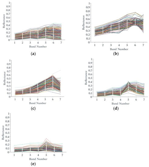
Figure 11.
Spectral curves of pixels (Threshold I: 0.85): (a) LIS, (b) HIS, (c) soil, (d) vegetation, and (e) water.
However, the spectral dataset of each type of ground object also contains the spectral characteristics of other ground objects (Figure 11), indicating that the ground objects (including impervious surface, vegetation, soil, and water) obtained by the above classification method are not reliable. Although the classification accuracy of the spectral dataset reaches the sub-pixel level and is filtered by Euclidean distance, there are still mixed phenomena. Figure 11d shows that the vegetation spectral dataset contains the spectral information of obvious soil and high-albedo impervious surfaces; Figure 11e shows that the water spectral dataset contains apparent vegetation spectral information.
In Figure 12, two detailed images are considered as examples. Considering the worldview image Figure 12(a1) as a reference and comparing Figure 12(a2) with Figure 12(a4) and Figure 12(a3) with Figure 12(a5), when the Threshold I value was 0.75, the impervious surface was significantly overestimated in the classification results of ResNet-18. Considering the worldview image Figure 12(b1) as a reference and comparing Figure 12(b2) with Figure 12(b3) and Figure 12(b4) with Figure 12(b5), the water pixels in the classification results of ResNet-18 with training datasets optimized based on the Euclidean distance could be better identified and extracted. The presence of mixed signals limits the accuracy of target features extracted by the LSMA and MNDWI threshold methods. In the mixed pixels, the reflection features of various ground objects affected each other. Therefore, in the mixed pixels, the spectral reflectance of the mixed pixels was not an exact linear combination of the endmember reflectance of various ground objects and their area ratios.

Figure 12.
Example of the results: (a1,b1) WorldView-2 images, (a2,b2) Experiment 1, (a3,b3) Experiment 2, (a4,b4) Experiment 3, and (a5,b5) Experiment 4.
5. Conclusions
Based on the actual spectrum of ground objects, a deep learning network, Resnet-18, was used to classify ground objects (vegetation, soil, IS, and water) in Landsat 8 OLI multispectral remote sensing images. In the classification of multispectral remote sensing images, to address the limitation of the large workload and non-negligible error of sample selection, the threshold, conventional LSMA, and spectral index methods were used to extract the spectral reflectance of certain ground object pixels. This was aimed at establishing a sample database required for deep learning and then building the Resnet-18 network to classify Landsat 8 multispectral remote sensing images. The results show that:
- Based on the traditional classification method, the spectral reflectance data of the pixels in the multispectral remote sensing image were extracted and then filtered by the Euclidean distance to establish a sample library supporting the classification of the deep learning model, which reduces the workload and errors of training sample selection.
- When using the spectral unmixing method to identify target objects in multispectral remote sensing images, owing to the similar spectral characteristics of the objects, spectral errors such as the same spectrum for different objects and varying spectra for the same objects occurred; errors occurred in the selection of pure pixels. Using deep learning methods to extract target objects in multispectral remote sensing images, the various spectral characteristics of target objects in multiple backgrounds can be fully considered, and these spectral errors can be reduced. When the spectral index was used to identify target objects in multispectral remote sensing images, the threshold selection was often biased owing to the strong subjectivity of the experimenter. Using deep learning methods to extract target objects in multispectral remote sensing images can reduce subjectivity and improve the classification.
- During the selection of the pixel spectrum, the principles based on deep learning and spectral unmixing were completely different: the higher the spectral purity of the pixel selected in spectral unmixing, the more conducive it was to the improvement of the accuracy of the unmixing result. In the deep learning model, pixel spectral information was used as a training sample, and the outlier of the spectral information of the target ground object also needed to be eliminated. However, certain amounts of spectral data are needed as samples for deep learning training to fully learn the spectral features of the target ground object and then carry out the classification of the ground object. In other words, incorporating all spectral features of all pixels of the target object to the extent possible is crucial.
The deep learning method often acts on hyperspectral and high-spatial-resolution remote sensing images and is rarely used for multispectral remote sensing images. This study presents a new concept for the establishment of a deep learning sample database and provides new insights and data support for the application of the deep learning model to multispectral remote sensing images. For further illustration of the suitability of deep learning for multispectral remote sensing images, future studies will use this method for the extraction of target objects and classification from global multitemporal multispectral remote sensing images (such as Landsat 9 and Sentinel 2 remote sensing images).
Author Contributions
Conceptualization, Y.Z.; methodology, Y.Z.; software, W.F.; validation, Y.Z.; formal analysis, Y.Z.; data curation, Y.Z.; writing—original draft preparation, Y.Z.; writing—review and editing, J.X. and X.Z.; visualization, Y.Z.; supervision, J.X. and X.Z.; project administration, X.Z.; funding acquisition, X.Z. All authors have read and agreed to the published version of the manuscript.
Funding
This research was funded by the National Natural Science Foundation of China, grant number 42071441.
Data Availability Statement
No new data were created or analyzed in this study. Data sharing is not applicable to this article.
Acknowledgments
The authors would like to thank USGS and ESPA for providing the research data, also thank the staff of editage for improving the language in the article. The authors are also grateful to the editors and anonymous reviewers for their positive comments on the manuscript.
Conflicts of Interest
The authors declare that they have no known competing financial interest or personal relationships that could have appeared to influence the work reported in this paper.
References
- Peng, W. Remote Sensing Instruction; Higher Education Press: Beijing, China, 2002; pp. 47–57. [Google Scholar]
- Tang, G. Remote Sensing Digital Image Processing; China Science Publishing & Media Ltd. (CSPM): Beijing, China, 2004. [Google Scholar]
- Liu, T.; Gu, Y.; Jia, X. Class-guided coupled dictionary learning for multispectral-hyperspectral remote sensing image collaborative classification. Sci. China Technol. Sci. 2022, 65, 744–758. [Google Scholar] [CrossRef]
- Zhao, Y.; Xu, J.; Zhong, K.; Wang, Y.; Hu, H.; Wu, P. Impervious Surface Extraction by Linear Spectral Mixture Analysis with Post-Processing Model. IEEE Access 2020, 8, 128476–128489. [Google Scholar] [CrossRef]
- Zhao, Y.; Xu, J.; Zhong, K.; Wang, Y.; Hu, H.; Wu, P. Impervious surface extraction based on Sentinel—2A and Landsat 8. Remote Sens. Land Resour. 2021, 33, 40–47. [Google Scholar] [CrossRef]
- Li, W. Mapping urban impervious surfaces by using spectral mixture analysis and spectral indices. Remote Sens. 2020, 12, 94. [Google Scholar] [CrossRef]
- Huete, A.; Didan, K.; Miura, T.; Rodriguez, E.P.; Gao, X.; Ferreira, L.G. Overview of the radiometric and biophysical performance of the MODIS vegetation indices. Remote Sens. Environ. 2002, 83, 195–213. [Google Scholar] [CrossRef]
- Rasul, A.; Balzter, H.; Ibrahim, G.R.F.; Hameed, H.M.; Wheeler, J.; Adamu, B.; Ibrahim, S.a.; Najmaddin, P.M. Applying built-up and bare-soil indices from Landsat 8 to cities in dry climates. Land 2018, 7, 81. [Google Scholar] [CrossRef]
- Spectroscopy Lab. Available online: https://www.usgs.gov/labs/spectroscopy-lab (accessed on 5 August 2022).
- Deng, Y. RNDSI: A ratio normalized difference soil index for remote sensing of urban/suburban environments. Int. J. Appl. Earth Obs. Geoinf. 2015, 39, 40–48. [Google Scholar] [CrossRef]
- Xu, H. A New Remote Sensing lndex for Fastly Extracting Impervious Surface Information. Geomat. Inf. Sci. Wuhan Univ. 2008, 33, 1150–1153+1211. [Google Scholar] [CrossRef]
- Xu, H. Analysis of Impervious Surface and its Impact on Urban Heat Environment using the Normalized Difference Impervious Surface Index (NDISI). Photogramm. Eng. Remote Sens. 2010, 76, 557–565. [Google Scholar] [CrossRef]
- Zha, Y.; Gao, J.; Ni, S. Use of normalized difference built-up index in automatically mapping urban areas from TM imagery. Int. J. Remote Sens. 2003, 24, 583–594. [Google Scholar] [CrossRef]
- Wang, Z.; Gang, C.; Li, X.; Chen, Y.; Li, J.; Gang, C.; Li, X.; Chen, Y.; Li, J. Application of a normalized difference impervious index (NDII) to extract urban impervious surface features based on Landsat TM images. Int. J. Remote Sens. 2015, 36, 1055–1069. [Google Scholar] [CrossRef]
- Deng, C.; Wu, C. BCI: A biophysical composition index for remote sensing of urban environments. Remote Sens. Environ. 2012, 127, 247–259. [Google Scholar] [CrossRef]
- Kawamura, M.; Jayamana, S.; Tsujiko, Y. Relation between social and environmental conditions in Colombo Sri Lanka and the Urban Index estimated by satellite remote sensing data. Int. Arch. Photogramm. Remote Sens. 1996, 31, 321–326. [Google Scholar]
- Xu, H. A study on information extraction of water body with the modified normalized difference water index (MNDWI). J. Remote Sens. 2005, 9, 589–595. [Google Scholar]
- Fan, F. The application and evaluation of two methods based on LSMM model—A case study in Guangzhou. Remote Sens. Technol. Appl. 2008, 023, 272–277. [Google Scholar]
- Weng, Q.; Lu, D. A sub-pixel analysis of urbanization effect on land surface temperature and its interplay with impervious surface and vegetation coverage in Indianapolis, United States. Int. J. Appl. Earth Obs. Geoinf. 2008, 10, 68–83. [Google Scholar] [CrossRef]
- Ridd, M.K. Exploring a V-I-S (vegetation-impervious surface-soil) model for urban ecosystem analysis through remote sensing: Comparative anatomy for cities†. Int. J. Remote Sens. 1995, 16, 2165–2185. [Google Scholar] [CrossRef]
- Zhang, H.; Lin, H.; Zhang, Y.; Weng, Q. Remote Sensing of Impervious Surfaces: In Tropical and Subtropical Areas; CRC Press: Boca Raton, FL, USA, 2015; pp. 10–12. [Google Scholar]
- Wu, C.; Murray, A.T. Estimating impervious surface distribution by spectral mixture analysis. Remote Sens. Environ. 2003, 84, 493–505. [Google Scholar] [CrossRef]
- Weng, Q. Remote sensing of impervious surfaces in the urban areas: Requirements, methods, and trends. Remote Sens. Environ. 2012, 117, 34–49. [Google Scholar] [CrossRef]
- Chen, Z.; Wu, W. A review on endmember extraction algorithms based on the linear mixing model. Sci. Surv. Mapp. 2008, 33, 49–51. [Google Scholar]
- Phinn, S.; Stanford, M.; Scarth, P.; Murray, A.T.; Shyy, P.T. Monitoring the composition of urban environments based on the vegetation-impervious surface-soil (VIS) model by subpixel analysis techniques. Int. J. Remote Sens. 2002, 23, 4131–4153. [Google Scholar] [CrossRef]
- Rashed, T.; Weeks, J.R.; Gadalla, M.S. Revealing the anatomy of cities through spectral mixture analysis of multispectral satellite imagery: A case study of the greater Cairo region, Egypt. Geocarto Int. 2001, 16, 5–15. [Google Scholar] [CrossRef]
- Wang, Q.; Lin, Q.; Li, M.; Wang, L. Comparison of two spectral mixture analysis models. Spectrosc. Spectr. Anal. 2009, 29, 2602–2605. [Google Scholar]
- Fan, F.; Wei, F.; Weng, Q. Improving urban impervious surface mapping by linear spectral mixture analysis and using spectral indices. Can. J. Remote Sens. 2015, 41, 577–586. [Google Scholar] [CrossRef]
- Zhao, Y.; Xu, J.; Zhong, K.; Wang, Y.; Zheng, Q. Extraction of urban impervious surface in Guangzhou by LSMA with NDBI. Geospat. Inf. 2018, 16, 90–93. [Google Scholar]
- Krizhevsky, A.; Sutskever, I.; Hinton, G. ImageNet classification with deep convolutional neural networks. Adv. Neural Inf. Process. Syst. 2012, 25. [Google Scholar] [CrossRef]
- Hinton, G.E.; Salakhutdinov, R.R. Reducing the dimensionality of data with neural networks. Science 2006, 313, 504–507. [Google Scholar] [CrossRef]
- Liu, C. Extraction Based on Deep Learning Supported by Spectral Library: Taking Qingdao as an Example. Master’s Thesis, Shandong University of Science and Technology, Qingdao, China, 2020. [Google Scholar]
- Feng, S.; Fan, F. Analyzing the effect of the spectral interference of mixed pixels using hyperspectral imagery. IEEE J. Sel. Top. Appl. Earth Obs. Remote Sens. 2021, 14, 1434–1446. [Google Scholar] [CrossRef]
- Wang, D.; Yang, R.; Liu, H.; He, H.; Tan, J.; Li, S.; Qiao, Y.; Tang, K.; Wang, X. HFENet: Hierarchical Feature Extraction Network for Accurate Landcover Classification. Remote Sens. 2022, 14, 4244. [Google Scholar] [CrossRef]
- Yu, J.; Zeng, P.; Yu, Y.; Yu, H.; Huang, L.; Zhou, D. A Combined Convolutional Neural Network for Urban Land-Use Classification with GIS Data. Remote Sens. 2022, 14, 1128. [Google Scholar] [CrossRef]
- Liu, R.; Tao, F.; Liu, X.; Na, J.; Leng, H.; Wu, J.; Zhou, T. RAANet: A Residual ASPP with Attention Framework for Semantic Segmentation of High-Resolution Remote Sensing Images. Remote Sens. 2022, 14, 3109. [Google Scholar] [CrossRef]
- Yu, J.; Du, S.; Xin, Z.; Huang, L.; Zhao, J. Application of a convolutional neural network to land use classification based on GF-2 remote sensing imagery. Arab. J. Geosci. 2021, 14, 1–14. [Google Scholar] [CrossRef]
- Karra, K.; Kontgis, C.; Statman-Weil, Z.; Mazzariello, J.C.; Mathis, M.; Brumby, S.P. Global land use/land cover with Sentinel 2 and deep learning. In Proceedings of the 2021 IEEE international geoscience and remote sensing symposium IGARSS, Brussels, Belgium, 11–16 July 2021; pp. 4704–4707. [Google Scholar]
- Parekh, J.; Poortinga, A.; Bhandari, B.; Mayer, T.; Saah, D.; Chishtie, F. Automatic Detection of Impervious Surfaces from Remotely Sensed Data Using Deep Learning. Remote Sens. 2021, 13, 3166. [Google Scholar] [CrossRef]
- Manickam, M.T.; Rao, M.K.; Barath, K.; Vijay, S.S.; Karthi, R. Convolutional Neural Network for Land Cover Classification and Mapping Using Landsat Images, Innovations in Computer Science and Engineering; Springer: Berlin/Heidelberg, Germany, 2022; pp. 221–232. [Google Scholar] [CrossRef]
- Mishra, V.K.; Swarnkar, D.; Pant, T. A Modified Neural Network for Land use Land Cover Mapping of Landsat-8 Oli Data. In Proceedings of the 2021 IEEE International India Geoscience and Remote Sensing Symposium (InGARSS), Ahmedabad, India, 6–10 December 2021; pp. 65–69. [Google Scholar] [CrossRef]
- Meerdink, S.K.; Hook, S.J.; Roberts, D.A.; Abbott, E.A. The ECOSTRESS spectral library version 1.0. Remote Sens. Environ. 2019, 230, 111196. [Google Scholar] [CrossRef]
- Baldridge, A.M.; Hook, S.J.; Grove, C.I.; Rivera, G. The ASTER spectral library version 2.0. Remote Sens. Environ. 2009, 113, 711–715. [Google Scholar] [CrossRef]
- ASU Thermal Emission Spectral Librar. Available online: http://tes.asu.edu/spectral/library/ (accessed on 5 August 2022).
- Mineral Spectral Server. Available online: http://minerals.gps.caltech.edu/ (accessed on 5 August 2022).
- CRISM Spectral Library. Available online: http://pds-geosciences.wustl.edu/missions/mro/spectral_library.htm (accessed on 5 August 2022).
- Bishop Spectral Library. Available online: https://dmp.seti.org/jbishop/spectral-library.html (accessed on 5 August 2022).
- Johns Hopkins University Spectral Library. Available online: http://speclib.jpl.nasa.gov/documents/jhu_desc (accessed on 5 August 2022).
- View_SPECPR: Software for Plotting Spectra (Installation Manual and User’s Guide, Version 1.2). Available online: http://pubs.usgs.gov/of/2008/1183/ (accessed on 5 August 2022).
- Li, W. Study on Extraction Method of Inland Surfacewater Body Based on Pixel Unmixing—A Case Study of Different Water Body Types in the Yellow River Basin. Master’s Thesis, Northwest University, Xi’an, China, 2017. [Google Scholar]
- Xu, J.; Zhao, Y.; Xiao, M.; Zhong, K.; Ruan, H. Relationship of air temperature to NDVl and NDBl in Guangzhou City using spatial autoregressive model. Remote Sens. Land Resour. 2018, 30, 186–194. [Google Scholar] [CrossRef]
- Xu, J.; Zhao, Y.; Zhong, K.; Zhang, F.; Liu, X.; Sun, C. Measuring spatio-temporal dynamics of impervious surface in Guangzhou, China, from 1988 to 2015, using time-series Landsat imagery. Sci. Total Environ. 2018, 627, 264–281. [Google Scholar] [CrossRef] [PubMed]
- Liao, P.; Chen, T.; Chung, P. A fast algorithm for multilevel thresholding. J. Inf. Sci. Eng. 2001, 17, 713–727. [Google Scholar]
- Ou, X.; Chang, Q.; Chakraborty, N. Simulation study on reward function of reinforcement learning in gantry work cell scheduling. J. Manuf. Syst. 2019, 50, 1–8. [Google Scholar] [CrossRef]
- He, K.; Zhang, X.; Ren, S.; Sun, J. “Deep Residual Learning for Image Recognition”. In Proceedings of the 2016 IEEE Conference on Computer Vision and Pattern Recognition (CVPR), Las Vegas, NV, USA, 27–30 June 2016; pp. 770–778. [Google Scholar] [CrossRef]


Publisher’s Note: MDPI stays neutral with regard to jurisdictional claims in published maps and institutional affiliations. |
© 2022 by the authors. Licensee MDPI, Basel, Switzerland. This article is an open access article distributed under the terms and conditions of the Creative Commons Attribution (CC BY) license (https://creativecommons.org/licenses/by/4.0/).