Article

Automatic Defect Detection of Pavement Diseases

College of Electronic and Information Engineering, Nanjing University of Aeronautics and Astronautics, Nanjing 211106, China
*
Author to whom correspondence should be addressed.
Remote Sens. 2022, 14(19), 4836; https://doi.org/10.3390/rs14194836
Submission received: 7 August 2022 / Revised: 16 September 2022 / Accepted: 21 September 2022 / Published: 28 September 2022

Abstract

:
Pavement disease detection is an important task for ensuring road safety. Manual visual detection requires a significant amount of time and effort. Therefore, an automated road disease identification technique is required to guarantee that city tasks are performed. However, due to the irregular shape and large-scale differences in road diseases, as well as the imbalance between the foreground and background, the task is challenging. Because of this, we created the deep convolution neural network—DASNet, which can be used to identify road diseases automatically. The network employs deformable convolution instead of regular convolution as the feature pyramid’s input, adds the same supervision signal to the multi-scale features before feature fusion, decreases the semantic difference, extracts context information by residual feature enhancement, and reduces the information loss of the pyramid’s top-level feature map. Considering the unique shape of road diseases, imbalance problems between the foreground and background are common, therefore, we introduce the sample weighted loss function. In order to prove the superiority and effectiveness of this method, it is compared to the latest method. A large number of experiments show that this method is superior in accuracy to other methods, specifically, under the COCO evaluation metric, compared with the Faster RCNN baseline, the proposed method obtains a 41.1 mAP and 3.4 AP improvement.

1. Introduction

The road starts with a single step, allows for convenient transportation, and provides an important guarantee for the operation of urban functions; however, each passage has an influence on the road. The influence of such activites are common concrete road cracks, potholes and rutting, looseness, subsidence, damage, and other issues, which, if not handled in time, can cause roads to become susceptible to deformation under various load types, such as vibration and shock [1], causing serious threats to road safety. This is due to the effect of the load of the road itself, building materials, construction error characteristics, and the external environment. The timely location and repair of pavement diseases is very important to maintain a road’s good running state. Therefore, it is necessary to carry out manual or automatic detection on a regular basis to detect the condition of the pavement. The majority of detection systems used to detect pavement disease both domestically and internationally are based on manual visual inspection, and have major drawbacks such as high inspection costs, low efficiency, low accuracy, and difficulty maintaining staff safety. Machine vision detection technology, a type of nondestructive testing technology used in many industrial domains, effectively eliminates the drawbacks of manual visual examination. It collects road images using a complementary metal oxide semiconductor (CMOS) camera or a charge coupled device (CCD) camera, and then utilizes the model to automatically identify faults [2,3,4]. The machine vision models used in such automatic techniques are acknowledged to be critical in assuring the effectiveness and accuracy of defect identification [5].
The introduction of machine vision has raised the bar for detecting pavement defects. Traditional machine vision methods can be divided into traditional image processing methods and machine learning methods. For example, in a study of road crack detection, Abdel Qader et al. [6] compared the performance of the fast Haar transform (FHT), the fast Fourier transform (FTT), the Sobel transform, and the Canny transform. It was determined that FHT was superior to other technologies based on the experimental results [5]. When detecting defects, the model based on mathematical morphology will perform corrosion, expansion, and other operations on the cracks in the road crack image [7,8], thereby improving the contrast of defects. However, the traditional machine vision model can not deal with defect detection against complex backgrounds because of the exposure, shade, advertisement occlusion, and other phenomena in the road disease image. Among the machine learning (ML) methods, various ML techniques based on shallow linear regression models, such as support vector machines (SVM) [9] and random forest (RF) [10], K-means [11], AdaBoost [12], regression analysis [13], grouping technique [14], restricted Boltzmann machine (RBM) [15,16], and other technologies have been applied successfully and satisfactorily in the defect identification processes of civil engineering projects [5]. The machine learning methods offer adaptable strategies for processing various road fracture patterns. However, the shallow linear regression model’s simplicity and real processing capability may limit the accuracy of the prediction. Deep convolutional neural networks (DNN), a set of probabilistic learning frameworks with low processing times, on the other hand, are appealing for real-time applications, and deep learning-based approaches have proven to be useful in numerous visual tasks.
Existing surface defects detection approaches based on DNN are essentially classified into two frameworks: single-stage and two-stage. The SSD (single shot multibox detector) [17] series and YOLO series [18] are examples of single-stage networks that employ only one network to identify areas of interest and output categories at the same time. This type of network is difficult to train and has low accuracy. Faster RCNN [19] is an example of a two-stage network, and its detection speed has substantially increased over the previous two generations. A two-stage network employs two subnetworks for location and classification, is simpler to train, and has higher overall accuracy than a single-stage network. However, due to the the intricacy of defects, when a two-stage network is employed for automatic road disease detection, there are two challenges: (1) Unlike in other applications, the shapes of the road diseases developed during usage are irregular, with substantial scale variances, as shown in Figure 1a–h, the eight diseases in the green box have different sizes and shapes; (2) Road diseases are typically irregular cracks. For some diseases with a big curvature, the detector’s determined region will contain too much background information, which might easily produce foreground–background imbalance and impact accuracy, as shown in Figure 1f–h. Here, the three types of diseases, patch-crack, patch-net, and pothole, contain too much background information in the green box, thereby increasing the likelihood of the foreground–background imbalance problem. The regular convolution layer is used in a conventional two-stage network. By extracting defect features with a fixed convolution kernel, it is easy to extract too much background information. Because the defect scales of road diseases are extremely varied, the regular convolution layer cannot adapt to these characteristics well. Furthermore, when adopting the conventional region proposal for foreground–background imbalance problems, the network is prone to focusing on “hard” samples, yet “hard” examples are not always significant. Therefore, it becomes critical to use a module with sample weighting and its related loss function in training to balance the link between classification and regression tasks.
To solve the aforementioned challenge, a high-quality defect detection framework termed DASNet is developed in this research. Our framework is based on Faster RCNN and is comprised of three well-designed modules: a deformable convolution-based feature extraction module, a new pyramid module, and a sample weighted loss function module. Figure 2 depicts the whole transmission path as well as the connectivity of the three modules. The following issues will be addressed mostly by cascading these three modules.
First, the deformable convolution module [20,21] is introduced to diverse shapes of road diseases. In comparison to the regular convolution grid, the deformed convolution module includes an offset layer parallel to the convolution layer. This allows the deformable convolution module to learn irregular shape offsets without further supervision. The feature extraction module may autonomously change the feature sample region throughout the inference process based on the shape information of distinct defects so that the features of the area of the defects include as little background information as possible.
Second, in the feature pyramid, enhancements are made to address the issue of underutilized multi-scale features in feature pyramid network (FPN) [22], first by consistency supervision to close the semantic gap before the fusion of features at various sizes. To limit information loss in the pyramid’s top-level feature map, feature fusion extracts proportionately invariant contextual information via residual feature augmentation. This phase can be intended to address the situation in which the detection accuracy of small-size defects has been diminished as a result of the introduction of deformable convolution.
Finally, a sample weighted loss function is employed during training to alleviate the foreground–background imbalance problem and increase detection accuracy. It predicts sample weight using the uncertainty distribution of samples in classification loss, regression loss, IOU, and probability score while avoiding some human parameter adjustments.
In summary, the contributions of this paper are as follows:
(1)
Deformable convolution and new feature pyramids are used to address irregular variations in defect shape and scale respectively.
(2)
Improved loss functions can improve detection accuracy.
(3)
Compared with benchmarks and other popular detectors (e.g., Cascade RCNN [23], RetinaNet [24], FCOS [25], ATSS [26], Libra RCNN [27], YOLOv3 [28], etc.), our model achieves state-of-the-art (SOTA) results on the COCO [29] mean Average Precision (mAP) metric.

2. Materials

2.1. Traditional Detection Methods

Both image processing-based and conventional machine learning methods are considered standard approaches in this field. The three types of image processing-based methods are threshold-based, edge detection, and feature-based.
Threshold-Based methods: In [30], scale space Gaussian blurring is used to preprocess the image of concrete cracks, and the Otsu threshold is calculated with differential image. A method to divide pavement crack image into two parts based on the Otsu threshold is proposed in [31]. In [32], Otsu image threshold segmentation technology was used to extract the characteristics of wormhole on concrete surface.
Edge detection algorithms: A threshold function is introduced into the Canny edge detection algorithm for pavement crack detection in [33]. A crack detection method, including a crack detection framework, is proposed in [34].
Features-Based methods: Using a Gabor filter to divide the pavement crack image into 128 × 128 sub-images in [35], and crack features are generated through a Gabor filter. Similarly, in [36], the Gabor filter is applied to a 30 × 40 non-overlapping window to generate bridge crack characteristics, which are then classified by SVM. The local binary pattern (LBP) is used to characterize the crack image features of pavement in [37]. In [38], the combination of symlet decomposition filter (SDF) and stationary wavelet transform (SWT) is used to preprocess pavement crack images, to reduce unnecessary texture in non-crack areas, and to enhance crack detection.
Machine learning methods: In [12], a supervised learning method based on AdaBoost is used to detect road cracks. Hierarchical clustering, K-means, and GMM (Gaussian Mixed Mode) clustering algorithms are used to cluster each block of pavement crack image in [39]. RF is improved in [40] to get a CrackForest method that includes integral channels to better represent the features of road cracks. K-nearest neighbor (KNN), SVM, RF, and neural network are used to identify pavement cracks and potholes in [41]. A fast classification method based on SVM is proposed in [42] for automatically detecting and quantifying defective patches of pavement. In [43], pavement potholes and cracks in aerial photography are classified in combination with SVM, artificial neural network (ANN) and RF. In [44], a probabilistic generation model (PGM) is combined with SVM to develop a pavement crack detection model based on a fused probability map. In [45], a feature extraction method based on image texture and the random gradient descent logistic regression method are used to automatically detect pavement diseases of asphalt pavement.

2.2. Deep Learning Methods

This section reviews the detection methods of pavement and concrete surface damage based on in-depth learning, which has achieved outstanding results in computer vision-related fields thanks to strong feature representation.
Classification: In [46], Applies a deep convolutional neural network (CNN) frame to road damage image classification. In [47], VGG-16 DCNN [48] is used to classify pavement image as “crack” or “no crack”. In [49], DCNN is used to classify pavement cracks on three-dimensional images and to mark these cracks in five different categories.
Location: In addition, YOLO v2, Faster RCNN and RetinaNet are often used to locate pavement lesions [50]. In [51], depth-based learning is used to locate crack areas.
Detection: A concrete crack detection model based on deep learning is presented in [52]. A CNN framework named NB-CNN is proposed in [53], in which naive Bayes data fusion technology is added to detect cracks from video frames. A five-layer CNN CrackNet architecture is suggested in [54] for the automatic detection of cracks in asphalt pavement. In [55], Faster-RCNN is used for crack detection.
Segmentation: In [56], a full convolution network (FCN) method is proposed for multiple damage types (cracks, peeling, holes, and weathering). In [57], semantic segmentation is introduced into a convolution network. A full convolution neural network (FCNN) is proposed for concrete crack detection based on expanding convolution to solve the problem of missing information during downsampling in concrete crack detection. The performance of CNN and FCN for pavement crack detection is compared in [58]. In [59], the top-down multi-level features are combined to segment pavement cracks. In [60], the depth of the convolution neural network and an improved image thinning algorithm to detect the crack in the dam slope protection is used.

2.3. Modern Object Detectors
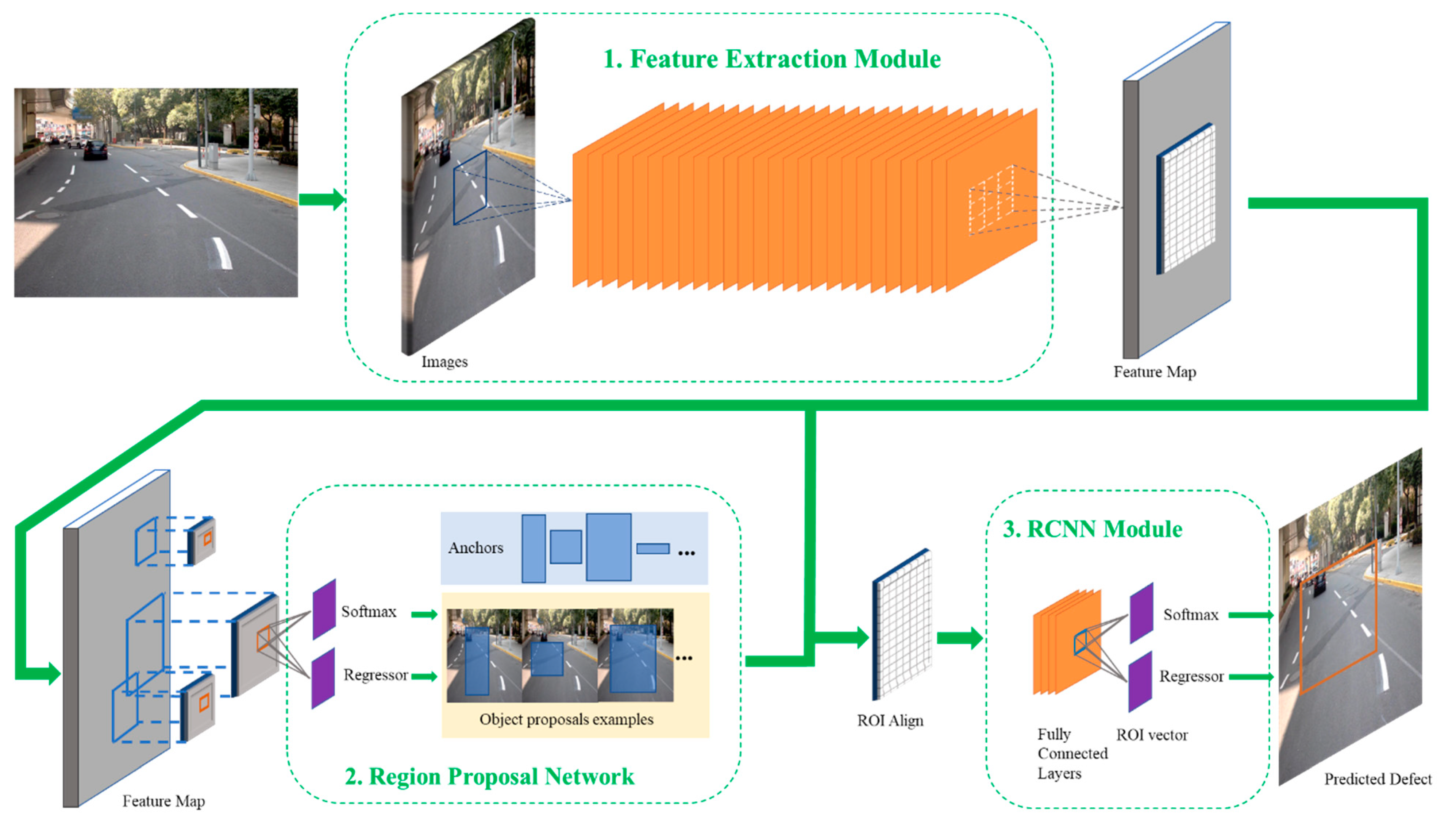
There are three types of modern object detectors: two-stage detectors, one-stage detectors, and anchor-free detectors. The two-stage detectors originate from RCNN [61]. The region of interest (ROI) is produced from the original image in the first stage. The ROI feature is extracted using the backbone network in the second stage. The ROI is then selected using Fast RCNN [62] and SPP-Net [63] from the feature extracted by the backbone network. Faster RCNN now generates ROI with a region proposal network (RPN). Because of the advent of Faster RCNN, the accuracy and speed of the two-stage detectors have substantially increased. As a result, these are now the most often used two-stage detectors, and are additionally used for milestone finding in object detection. Two-stage detectors have variations such as Cascade RCNN, Grid RCNN [64], and Libra RCNN. The one-stage detectors’ RPN can be fused with the classifier to immediately classify and regress the bounding box through the neural network. This works faster but is less accurate than two-stage detectors such as YOLO and RetinaNet. Anchor-free detectors, represented by FCOS and ATSS, have developed significantly over the last two years, require no bounding boxes, and are simple to calculate.

2.4. Faster RCNN

The RCNN family of object detection algorithms works by first generating certain region proposals, which are subsequently classified and positioned using regression. Faster RCNN achieves end-to-end training [65] and significantly increases speed by replacing previous RCNN algorithms that produce region proposals using Selective Search (SS) techniques with neural networks. Thanks to these advantages, DASNet is expanded on the basis of the three components of Faster RCNN. As shown in Figure 3, Faster RCNN mainly consists of three modules: feature extraction module, area RPN, and RCNN module (that is, Roi Align and classification network).
(1)
Module for feature extraction. The feature map of the image is first extracted using a set of basic conv + relu + pooling layers. This feature map is then shared for subsequent RPN layers and fully connected layers.
(2)
The RPN network is actually divided into two lines, one is used to obtain the positive and negative classification by softmax classification anchors, and the other is used to calculate the bounding box regression offset relative to anchors to obtain the accurate proposal. It is equivalent to completing the function of target positioning.
(3)
The RCNN module (i.e., Roi Align and classification network. In order to avoid the mis-alignment problem caused by the two quantizations in the Roi Pooling operation, Roi Align is used instead of the original Roi Pooling) is used to classify the candidate detection boxes. And after the RPN, the coordinates of the candidate box are fine-tuned again to output the detection results.

2.5. FPN

In object detection, convolutional networks often have some technical drawbacks: although high-level networks can contain semantic features, they do not have much geometric information, which is not conducive to object detection. Although the shallow network contains more geometric information, there are not many semantic features of the image, which is not conducive to image classification. This problem is more prominent in small object detection. A common scheme is to build a pyramid [66]. Pyramids need to distinguish simple objects by using shallow features, and complex objects by using deep features [67]. However, in practical applications, the pyramid is often directly obtained from the shallow layer of the network, which leads to the loss of some semantic information. FPN [22] uses the pyramid form of CNN hierarchical features [68] to generate feature pyramids with strong semantic information at all scales. FPN uses bottom-up path, top-down path, and lateral connection mode. In this way, feature gold characters of each scale with strong semantic information can be quickly constructed from the input image of a single scale.

3. Methods

The DASNet defects detection framework is proposed by deformable convolution module, feature pyramid module, and loss function module, as shown in Figure 2. There are a few important differences between Faster RCNN and this version. To obtain feature maps, deformable convolutions were originally introduced to replace regular convolutions. Then, using an upgraded pyramid module, feature enhancement is achieved by combining all feature maps of various resolutions. Finally, the sample weighted loss function module is used to modify the predicted bounding box to solve the foreground–background imbalance problem in Faster RCNN processing of pavement diseases.

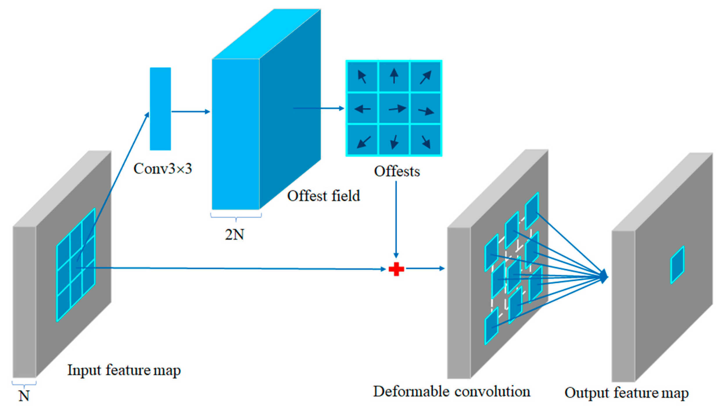
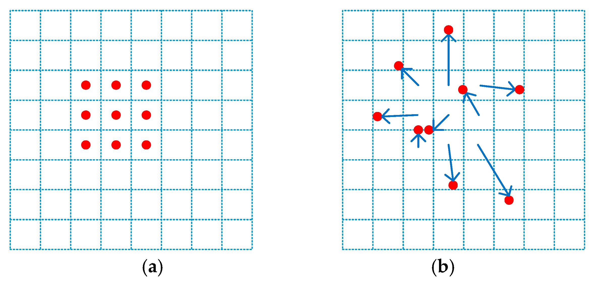
3.1. Deformable Convolution

When convolution is performed using conventional convolutional computation rules, it cannot change adaptively with object scaling, rotation, or irregular shape, but by observing deformable convolution, which can effectively march and deform according to the target geometry when facing irregular targets. As inspired by the literature [20,21], we apply deformable convolution to replace the original regular convolution in the feature extraction module. As features are learned, the shape of the sampled region can be changed adaptively, as can be seen in Figure 4. As part of the deformable convolution operation on the feature map, a new 3 × 3 convolution layer (i.e., the upper part of the figure) is defined after the input feature map to learn the position offsets with the same output dimension as the original feature map and several channels of 2N, representing the offsets in the x, y direction. Following this, the learned offsets are inserted into the input feature mapping by bilinear interpolation before the result is passed to the deformable convolution layer.
With DCNv2, convolution is a two-dimensional operation, and the input feature map is sampled by using 3 × 3 grids R (that is, convolution kernels) that differ from the grids found in regular convolution by adding position offsets to the traditional grids, as shown in Figure 5. Thus, for each position p0 on the resulting feature map, the matrix obtained from the deformable convolution kernel can be expressed as follows:
y p 0 = p n R w p n · x p 0 + p n + p n
where p n lists the positions in R, p n p n | n = 1 , 2 , , N ,   N = R is the position offset, and R is the augmentation of p n .

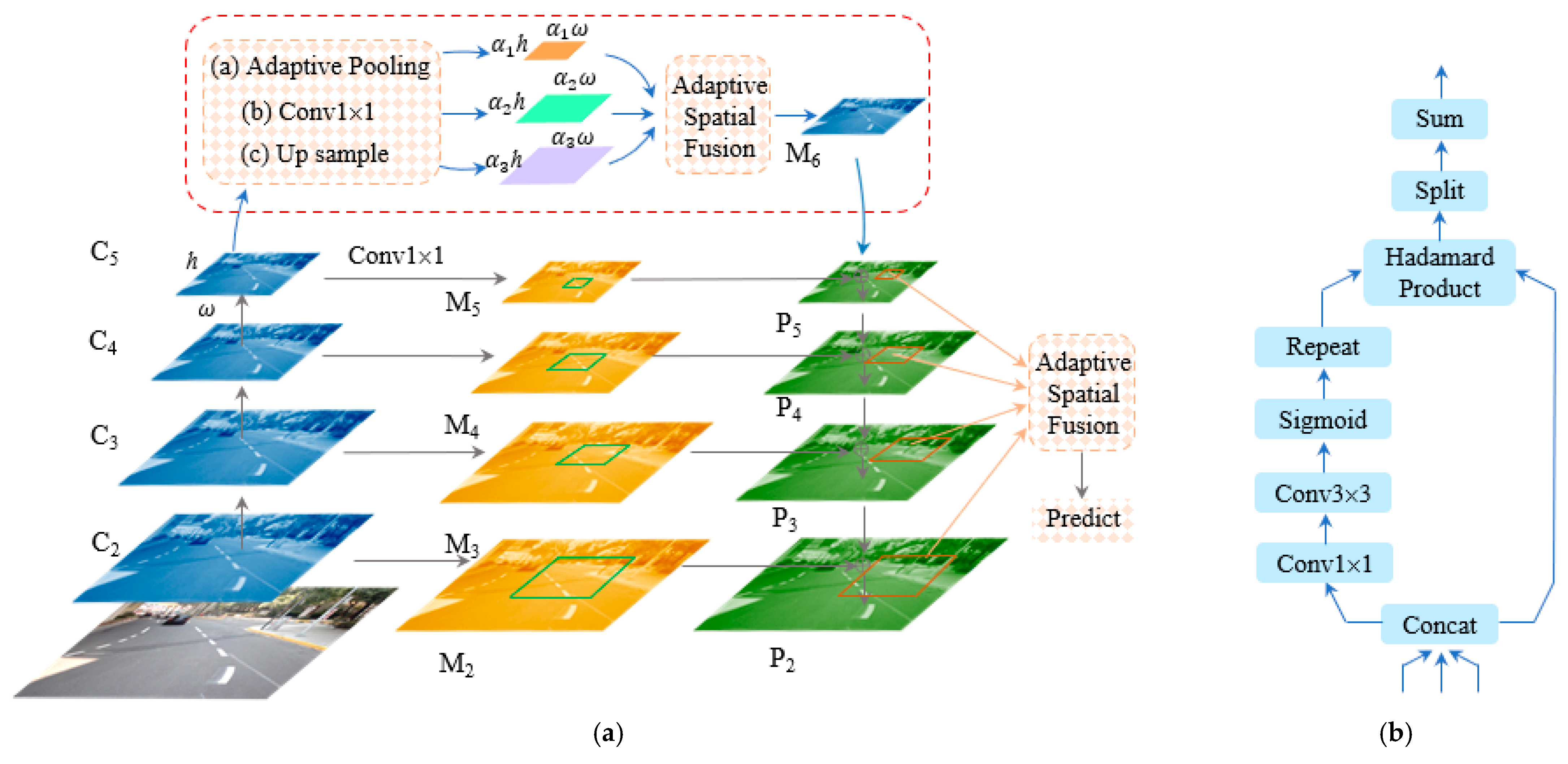
3.2. Aug Feature Pyramid Module

The FPN [22], which contains a top-down pipeline and some lateral connections, is used to fuse neighboring feature maps to generate a multi-scale feature map, as shown in Figure 6a. When road diseases at different scales enter the network, they are divided into different pyramid layers, with the bottom feature scale being large and containing only some information such as edges and corner points, and the top feature scale being small and containing more semantic information. The FPN has design flaws: it directly fuses features at different scales, ignoring the large semantic gap between them; the top-down feature fusion approach causes the top layer features to be lost. All these flaws result in sub-optimal pyramids. A heuristic idea is, therefore, elicited to add the same supervised signal to multi-scale features before feature fusion to reduce the semantic gap, and a Residual Feature enhancement (RFE) method is proposed to improve the feature representation of M5 by injecting different spatial contextual information into the original branch using residual branches.
In this paper, AugFPN [69] is used to further enhance the feature and improve the detection accuracy by using the consistent supervision and residual feature enhancement module. The specific workflow is shown in Figure 6, which mainly includes the following steps:
(1)
First, a feature pyramid {P2, P3, P4, P5} is constructed based on the multi-scale features {C2, C3, C4, C5} obtained from the backbone, and detectors and classifiers, i.e., RPN Head and RCNN, are added to each feature before it enters the feature pyramid fusion, as shown in the middle part of Figure 6a, which maps the ROIs generated by RPN onto {M2, M3, M4, M5} and obtains the corresponding feature maps to classify and regress these features. The parameters of these classification and regression heads are shared at different levels, facilitating the supervision of features at different scales.
(2)
Using residual branches to inject different spatial contextual information into the original branches to improve the feature representation of M5. Assuming that the size of C5 is S = h × w, we downsample C5 into 3 copies, respectively. Specifically, as shown in Figure 6a. Firstly, sample C5 as α1 × s, α2 × s, and α3 × s respectively by adaptive pooling. Secondly, convolve the results of adaptive pooling into 1 × 1 respectively to bring the feature channel down to 256. Thirdly, upsample the 3 different downsampled results again (scale with C5 to remain consistent at 256) as adaptive spatial fusion input.
(3)
The next step is adaptive spatial fusion and the final generation of a spatial weight for each feature. This is shown in Figure 6b, where the α1 × s, α2 × s and α3 × s are concat, and finally, the contextual features are fused into M6 using the weights. After generating M6, it is summed with M5 and fused with other lower-level features in turn by propagation. After fusion, 3 × 3 convolution is performed on each feature vector to build the feature pyramid {P2, P3, P4, P5}.

3.3. Sample Weighted Loss Function Module

Pavement images usually contain a variety of diseases. When detecting based on regions, some common diseases (such as cracks) have a large curvature, which can easily lead to too much background information in the bounding box, causing foreground–background imbalance. To further improve the detection accuracy, a sample weighted module is proposed to calculate the loss, and the original loss function in Faster RCNN is improved. According to [70], this sample weighted module jointly learns the sample weights for classification and regression tasks, which can achieve good performance gains without affecting the inference time of the Faster RCNN. The sample weighted module is built based on the multilayer perceptron (MLP), as shown in Figure 7. It combines classification loss, regression loss, IOU, and classification score, exploiting the relationship between these four in terms of uncertainty in response prediction and avoiding the corresponding loss of true values due to the direct use of visual features.
Specifically, for the ith sample, the regression task is modeled as a Gaussian likelihood, so the mean and standard deviation σireg of the offset between the ground truth and the predicted position has the following relationship:
  p g t i | a i * = N a i * , σ i r e g 2
where the vector gti represents the ground truth of boundary box coordinates, and a* represents the predicted value of bounding box coordinates. Maximize the logarithmic probability of likelihood to optimize the regression network:
l o g p g t i | a i * 1 σ i r e g 2 | | g t i a i * | | 2 2 l o g σ i r e g
A further, defining L i r e g * = | | g t i a i * | | 2 2 , Equation (2) can be arranged as follows:
L i r e g * = 1 σ i r e g 2 L i r e g + λ 2 l o g σ i r e g
where λ2 is a constant used to balance weights. It can be seen from Equation (4) that with the increase of offset, the weight on Lireg decreases. Therefore, this strategy places more weight on confident samples and imposes more penalties on the mistakes made by these samples in the training process.
Classification loss is consistent with regression loss, then:
L i c l s = l o g   s o f t m a x y i , p a i *
The classification loss is approximated by:
L i c l s * = 1 σ i c l s 2 L i c l s + λ 1 l o g σ i c l s
The overall weighted loss is:
L i = L i c l s * + L i r e g * = 1 σ i c l s 2 L i c l s + 1 σ i r e g 2 L i r e g + λ 1 l o g σ i c l s + λ 2 l o g σ i r e g
Let m i · = l o g σ i · , the overall weighted loss after optimization is:
L i = e x p 2 m i c l s L i c l s + λ 1 m i c l s + e x p 2 m i r e g L i r e g + λ 2 m i r e g
where m i · can be obtained by learning feature di, as shown in Equation (9), and di is defined by Equation (10):
m i c l s = W c l s d i m i r e g = W r e g d i
d i = c o n c a t F L i c l s ; G L i r e g ; H I o U i ; K P r o b i
W c l s and W r e g respectively represent different MLP, indicating that feature di is learned from two independent MLP to obtain the corresponding m i · . The di is obtained by combining classification loss, regression loss, IoU, and scoring probability by using the correlation between offset and ground truth.

4. Experiments and Results

We have conducted in-depth experiments on the challenging pavement dataset and evaluated our approach.

4.1. Dataset

The pavement dataset used in this paper is derived from the “Global Open Data Innovation Competition”. It contains 8 disease types and 14,000 road disease images of different scales and resolutions. The training set allocates 6000 pictures; test set A allocates 2000 pictures and test set B allocates 6000 pictures. Figure 8 shows some examples of the dataset.

4.2. Evaluation Metrics

A confusion matrix is frequently utilized in the evaluation of object detection models as an essential indication. Table 1 depicts the association between TP (true positive), FN (false negative), FP (false positive), and TN (true negative). Using the confusion matrix indications as a starting point, new assessment indicators appropriate for diverse purposes may be generated through combination. Table 2 displays the key indicators. Table 3 lists some definitions of accuracy, and all the experimental results in this paper are measured using COCO. In this experiment, we assessed the mean accuracy at various IoU thresholds, with a range of 0.5 to 0.95 and a 0.05 interval. This reflects the performance of detection under various criteria and has a high level of local detection result accuracy.

4.3. Experimental Details

All experiments were implemented based on MMdetection [72]. The operating system is ubuntu20.04 (Canonical, London, UK) and the graphics card is NVIDIA GeForce RTX 3090 (Santa Clara, CA, USA). By default, we trained the model with 1 GPU (3090) for 24 epochs, which is commonly referred to as 2× training schedule. Initialization parameters for feature extraction networks such as ResNet-50 [73], ResNet-50-FPN, and ResNet-50-DCNv2 (only those with a depth of 50 are provided below, with reference values for other network parameters in depth) are translated from the ImageNet dataset training model. Other advanced methods utilized to compare detection performance in this research make advantage of the pre-training weights given by MMdetection. To train the detection network, all approaches in this research employed the stochastic gradient descent method (SGD). The initial learning rate was set to 0.0025 and declined at a rate of 0.1 after the 8th and 11th iterations. A weight decay of 0.0001 was used for optimizers. In addition, λ1 and λ2 were all taken as 0.5, and all other hyperparameters in this paper follow MMdetection.

4.4. Experimental Results

To verify the effectiveness of the proposed performance enhancement methods, Faster RCNN and the proposed models were comprehensively evaluated on ResNet-50 and ResNeXt-101-32×4d [74]. Because the DASNet has a pyramid module, the Faster RCNN is equipped with a FPN for fairness. Table 4 shows the test results for average accuracy (AP) on the road dataset. It can be seen that DASNet, with Resnet-50 as the backbone, has 40.1% mAP and 2.4% higher mAP than Faster RCNN due to its well-designed modules. DASNet can still improve the performance of Faster RCNN by 5.0% when using stronger backbone networks such as ResNeXt-101-32×4d. In contrast, DASNet shows better classification and positioning performance for targets of different scales. The inference time of each image processed by Faster RCNN and DASNet is also compared in Table 4. Despite the fact that adding the intended module to the baseline will lengthen the inference time, DASNet (0.3 s/image) can still complete real-time detection tasks in the required time.
Figure 9 shows different road disease samples, each of which can be correctly detected. Figure 10 shows our method and the performance of some SOTA object detection detectors on each disease category. To be fair, the SOTA methods shown in Figure 10 are all ResNet-50 with FPN except Darknet-53, which is the backbone network of YOLOv3. Specifically, in Figure 10a, the detection accuracy of our method for each disease type is shown. It can be seen that the detection accuracy of most diseases is very high, but there are also some differences between different disease types, such as “other” type and “manhole” type. In multitask detection, the network will concentrate its attention on some samples with large classification loss (i.e., ‘hard’ samples), which will easily sacrifice the positioning ability of the network for accuracy, resulting in a reduction in accuracy. When the IoU is larger than 0.5, improper positioning has a bigger impact on average accuracy. The detection accuracy of other SOTA approaches varies by illness category, as illustrated in Figure 10e. The distinction is larger than that of our technique. DASNet contains a sample weighting module, which enables the sample weights to be consistent between different tasks. It prevents some networks from paying too much attention to “hard” samples and reduces some weights of “easy” samples, which affects the overall detection accuracy. At an IoU of 0.75, the accuracy decreases less than Faster RCNN. At the same time, the fusion of semantic information by the pyramid module in DASNet makes the extracted features contain more detailed information, and also contributes to the accuracy of disease detection for each category. From Figure 10b–d, we can see that our method is based on Faster RCNN, but the detection accuracy of each disease category has been improved. Overall, the detection performance of DASNet is better than other networks.

4.5. Ablation Experiments

Overall ablation studies. A series of ablation studies were implemented in order to analyze the importance of these proposed components. As shown in Table 5, the feature extraction network uses Resnet-50, with deformable convolution, AugFPN, and sample weighted loss function (SWLF) progressively added on top of Faster RCNN, ‘√’ means adding the corresponding module. Three useful conclusions can be drawn from the results in Table 5. First, with the addition of DCN, mAP, AP50, AP70, and APl all increase, but the detection performance of medium and small defects decreases; AugFPN better integrates the characteristic maps of different scales, so that each index was improved. It can be seen that adding AugFPN to the existing DCN network significantly improved the detection accuracy of small and medium-sized targets, and the network performance was significantly improved. Second, SWLF also improves the network accuracy and is friendlier to larger targets. Third, by adding these three modules in turn, the evaluation criteria, such as mAP, were improved.
Deformable convolutional ablation study. Using the Faster RCNN with a backbone of ResNet50 as a benchmark, it can be seen from Table 5 that the deformable convolutional network (DCN) is 0.7 points higher than the benchmark AP. To demonstrate the advantage in deformable convolutional performance, we configured DCNs to feature extraction networks of different depths for comparison, and the results are shown in Table 6 compared with Resnet-50, Resnet-101, and ResneXt-101 have a deeper network hierarchy, larger model prediction capacity, and higher performance. In addition, it should be noted that deformable convolution greatly improves performance both on efficient models like Resnet-50 and on complex networks like ResneXt-101. Additionally, it should be noted that the DCN configuration on Resnet-50 was improved according to most indicators, but its accuracy in detecting small defects is not high. Gradually, APs starts to converge with the benchmark as the feature extraction network gets deeper.
AugFPN ablation study. For comparison, we re-implemented the corresponding FPN-based benchmark method. The results are shown in Table 7, where the Faster RCNN incorporating AugFPN and using ResNet-50 as the backbone (denoted ResNet-50-AugFPN) obtained 39.8 mAP, which is 1.1 points higher than the mAP of ResNet-50-FPN, Aps and APm also increased by 0.9 and 3.8 points, respectively. Furthermore, even when the Faster RCNN is selected over a more robust backbone, the AugFPN consistently delivers non-negligible performance. For example, when using ResNeXt-101 as a feature extraction network, AugFPN still improved performance by 2.7 points over FPN’s mAP.
Sample Weighted Loss Function ablation study. Using Faster RCNN + ResNet-50 as a benchmark. The results are shown in Table 8, where it is shown that the performance of each network has been steadily improved with the addition of the SWLF module. Among them, mAP, APs and APm increased by 0.8, 1.4, and 4.7, respectively.

4.6. Comparison with Other Object Detection Algorithms

On the road dataset, we compare the proposed approach to other SOTA object detection detectors. All SOTA detector re-implementations are subject to the published studies, and only the hyperparameters are fine-tuned using the road dataset. The experimental results are shown in Table 9. The following conclusions can be drawn from the experimental results:
(1)
In the first group, compared with some advanced algorithms, including one-stage and two-stage detectors, our method map reaches 41.1%, which is better than the above methods by 3.4–7.6%.
(2)
In the second group, the FPN is added to the detectors to create a multi-level detector, which is extensively employed in object detection and has the potential to considerably increase the detectors’ performance. Our technique incorporates an enhanced FPN, which improves detector performance by 2.4–8% mAP over the method with FPN (Remove FCOS and Libra RCNN with poor results). Moreover, our method is higher in AP50 and improved in AP75, showing good classification and positioning performance, and improving target detection performance in different sizes.
(3)
In the third group, our method’s robustness is demonstrated. Several FPN-adding technologies have been chosen to upgrade their backbone to the stronger ResNet-101. Our method’s mAP was elevated by 17.8%, which is 5.4–27.4% mAP greater than the SOTA detector. The discrepancy between our solution and the other SOTA solutions is the same as prior to the backbone update.

5. Conclusions

To address the challenge of quality identification in road applications, the DASNet surface defect detection method is introduced. The technique, which is based on Faster RCNN, employs a two-stage detector, meticulously develops three components. In addition, deformable convolution modules, AugFPN modules, and sample weighted loss functions that may learn task weights are used in our system to address the issues of road surface disease identification. This approach may be used to assess irregular form pavement diseases, particular types of defects, and accurate placement, giving detailed and useful indications for the quality control process, such as number of defects, category, area, and location. Experiments reveal that this method’s mAP value is 41.1 percent on the public road diseases dataset, and it outperforms other object identification approaches in terms of accuracy.
Our current work has shortcomings in accuracy and generalization, and has the problem of weak transferability in practical applications. At the same time, only urban pavement diseases were deeply studied. In addition to urban pavement disease, there are concrete diseases such as bridge surface and tunnel surface. In our future work, we will employ the following methods. First, we will use an unmanned aerial vehicle (UAV) to collect more kinds of defect images to expand our research objects and improve the generalization of our work. Second, we will collect more datasets with complex backgrounds to improve the accuracy and robustness of the model. Thirds, we will adjust the model, apply transfer learning to detect more types of diseases with the help of better performance models, and also consider constructing an effective and lightweight feature extraction network in the case of unsupervised learning. Fourth, we will conduct segmentation research on the disease contours to help researchers understand the damage degree of the diseases.

Author Contributions

Conceptualization, L.Z.; methodology, L.Z.; software, L.Z.; validation, L.Z. and Y.Y.; formal analysis, L.Z. and X.L.; investigation, X.L.; resources, L.Z. and Y.Y.; data curation, L.Z. and Y.Y.; writing—original draft preparation, L.Z. and Y.Y.; writing—review and editing, L.Z.; visualization, L.Z., X.L. and Y.Y.; supervision, Y.W.; project administration, Y.W.; funding acquisition, Y.W. All authors have read and agreed to the published version of the manuscript.

Funding

This research was funded by the National Nature Science Founding of China under Grant 61573183.

Data Availability Statement

Conflicts of Interest

All authors declare no conflict of interest.

References

  1. Tang, Y.; Zhu, M.; Chen, Z.; Wu, C.; Chen, B.; Li, C.; Li, L. Seismic performance evaluation of recycled aggregate concrete-filled steel tubular columns with field strain detected via a novel mark-free vision method. Structures 2022, 37, 426–441. [Google Scholar] [CrossRef]
  2. Yu, S.N.; Jang, J.H.; Han, C.S. Auto inspection system using a mobile robot for detecting concrete cracks in a tunnel. Autom. Constr. 2007, 16, 255–261. [Google Scholar] [CrossRef]
  3. Zhang, W.; Zhang, Z.; Qi, D.; Liu, Y. Automatic crack detection and classification method for subway tunnel safety monitoring. Sensors 2014, 14, 19307–19328. [Google Scholar] [CrossRef]
  4. Fukuda, Y.; Feng, M.Q.; Narita, Y.; Kaneko, S.; Tanaka, T. Vision based displacement sensor for monitoring dynamic response using robust object search algorithm. Sensors 2013, 13, 4725–4732. [Google Scholar] [CrossRef]
  5. Miao, X.; Wang, J.; Wang, Z.; Sui, Q.; Gao, Y.; Jiang, P. Automatic Recognition of Highway Tunnel Defects Based on an Improved U-Net Model. Sensors 2019, 19, 11413–11423. [Google Scholar] [CrossRef]
  6. Abdel-Qader, I.; Abudayyeh, O.; Kelly, M.E. Analysis of edge detection techniques for crack identification in bridges. J. Comput. Civ. Eng. 2003, 17, 255–263. [Google Scholar] [CrossRef]
  7. Tanaka, N.; Uematsu, K. A crack detection method in road surface images using morphology. Proc. MVA 1998, 98, 17–19. [Google Scholar]
  8. Iyer, S.; Sinha, S.K. Segmentation of pipe images for crack detection in buried sewers. Comput.-Aided Civ. Infrastruct. Eng. 2006, 21, 395–410. [Google Scholar] [CrossRef]
  9. Burges, C.J.C. A tutorial on support vector machines for pattern recognition. Data Min. Knowl. Discov. 1998, 2, 121–167. [Google Scholar] [CrossRef]
  10. Breiman, L. Random forests. Mach. Learn. 2001, 45, 5–32. [Google Scholar] [CrossRef]
  11. Lattanzi, D.; Miller, G.R. Robust automated concrete damage detection algorithms for field applications. J. Comput. Civ. Eng. 2012, 28, 253–262. [Google Scholar] [CrossRef]
  12. Cord, A.; Chambon, S. Automatic road defect detection by textural pattern recognition based on AdaBoost. Comput.-Aided Civ. Infrastruct. Eng. 2012, 27, 244–259. [Google Scholar] [CrossRef]
  13. Dawood, T.; Zhu, Z.; Zayed, T. Machine vision-based model for spalling detection and quantification in subway networks. Automat. Construct 2017, 81, 149–160. [Google Scholar]
  14. Yeum, C.M.; Dyke, S.J. Vision-based automated crack detection for bridge inspection. Comput.-Aided Civ. Infrastruct. Eng. 2015, 30, 759–770. [Google Scholar] [CrossRef]
  15. Rafiei, M.H.; Adeli, H. A novel unsupervised deep learning model for global and local health condition assessment of structures. Eng. Stuctures 2018, 156, 598–607. [Google Scholar] [CrossRef]
  16. Rafiei, M.H.; Khushefati, W.H.; Demirboga, R.; Adeli, H. Supervised deep restricted Boltzmann machine for estimation of concrete. ACI Mater. J. 2017, 114, 237–244. [Google Scholar] [CrossRef]
  17. Liu, W.; Anguelov, D.; Erhan, D.; Szegedy, C.; Reed, S.; Fu, C.Y.; Berg, A.C. SSD: Single shot multibox detector. In Proceedings of the 14th Europeon Conference on Computer Vision (ECCV), Amsterdam, The Netherlands, 11–14 October 2016; pp. 21–37. [Google Scholar]
  18. Redmon, J.; Divvala, S.; Girshick, R.; Farhadi, A. You only look once: Unified, real-time object detection. In Proceedings of the 2016 IEEE Conference on Computer Vision and Pattern Recognition (CVPR), Seattle, WA, USA, 27–30 June 2016; pp. 779–788. [Google Scholar]
  19. Suh, G.; Cha, Y.J. Deep faster R-CNN based automated detection and localization of multiple types of damage. In Proceedings of the Sensors and Smart Structures Technologies for Civil, Mechanical, and Aerospace Systems, Online, 27 April–8 May 2020; SPIE: Bellingham, WA, USA, 2018; Volume 10598, p. 105980T. [Google Scholar] [CrossRef]
  20. Dai, J.; Qi, H.; Xiong, Y. Deformable Convolutional Networks. In Proceedings of the 16th IEEE International Conference on Computer Vision (ICCV), Venice, Italy, 22–29 October 2017; pp. 764–773. [Google Scholar]
  21. Zhu, X.; Hu, H.; Lin, S.; Dai, J. Deformable ConvNets V2: More Deformable, Better Results. In Proceedings of the 2019 IEEE/CVF Conference on Computer Vision and Pattern Recognition (CVPR), Long Beach, CA, USA, 15–20 June 2019; pp. 9300–9308. [Google Scholar]
  22. Lin, T.Y.; Dollár, P.; Girshick, R.; He, K.; Hariharan, B.; Belongie, S. Feature pyramid networks for object detection. In Proceedings of the 30th IEEE/CVF Conference on Computer Vision and Pattern Recognition (CVPR), Honolulu, HI, USA, 21–26 July 2017; pp. 2117–2125. [Google Scholar]
  23. Cai, Z.W.; Vasconcelos, N. Cascade R-CNN: Delving into high quality object detection. In Proceedings of the 31st IEEE/CVF Conference on Computer Vision and Pattern Recognition (CVPR), Salt Lake City, UT, USA, 18–23 June 2018; pp. 6154–6162. [Google Scholar]
  24. Lin, T.Y.; Goyal, P.; Girshick, R.; He, K.; Dollár, P. Focal loss for dense object detection. IEEE Trans. Pattern Anal. Mach. Intell. 2017, 99, 2999–3007. [Google Scholar] [CrossRef]
  25. Tian, Z.; Shen, C.; Chen, H.; He, T. FCOS: Fully convolutional one-stage object detection. In Proceedings of the IEEE/CVF International Conference on Computer Vision (ICCV), Seoul, Korea, 27 October–2 November 2019; pp. 9626–9635. [Google Scholar]
  26. Zhang, S.; Chi, C.; Yao, Y.; Lei, Z.; Li, S.Z. Bridging the gap between anchor-based and anchor-free detection via adaptive training sample selection. In Proceedings of the 33rd IEEE/CVF Conference on Computer Vision and Pattern Recognition (CVPR), Seattle, WA, USA, 13–19 June 2020; pp. 9756–9765. [Google Scholar]
  27. Pang, J.; Chen, K.; Shi, J.; Feng, H.; Ouyang, W.; Lin, D. Libra R-CNN: Towards balanced learning for object detection. In Proceedings of the 32nd IEEE/CVF Conference on Computer Vision and Pattern Recognition (CVPR), Long Beach, CA, USA, 16–20 June 2019; pp. 821–830. [Google Scholar]
  28. Redmon, J.; Farhadi, A. YOLOv3: An Incremental Improvement. arXiv 2018, arXiv:1804.02767. Available online: http://arxiv.org/abs/1804.02767 (accessed on 7 August 2022).
  29. Lin, T.Y.; Maire, M.; Belongie, S.; Hays, J.; Perona, P.; Ramanan, D.; Dollar, P.; Zitnick, C.L. Microsoft COCO: Common objects in context. In Proceedings of the 13th European Conference on Computer Vision (ECCV), Zurich, Switzerland, 6–12 September 2014; pp. 740–755. [Google Scholar]
  30. Chen, B.; Zhang, X.; Wang, R.; Li, Z.; Deng, W. Detect concrete cracks based on OTSU algorithm with differential image. J. Eng. 2019, 23, 9088–9091. [Google Scholar] [CrossRef]
  31. Quan, Y.; Sun, J.; Zhang, Y.; Zhang, H. The Method of the Road Surface Crack Detection by the Improved Otsu Threshold. In Proceedings of the 2019 IEEE International Conference on Mechatronics and Automation (ICMA), Tianjin, China, 4–7 August 2019; pp. 1615–1620. [Google Scholar]
  32. Liu, X.; Xue, F.; Teng, L. Surface defect detection based on gradient LBP. In Proceedings of the 2018 IEEE 3rd International Conference on Image, Vision and Computing (ICIVC), Chongqing, China, 27–29 June 2018; pp. 133–137. [Google Scholar]
  33. Gunawan, G.; Nurdiyanto, H.; Sriadhi, S.; Fauzi, A.; Usman, A.; Fadlina, F.; Dafitri, H.; Simarmata, J.; Siahaan, A.; Rahim, R. Mobile Application Detection of Road Damage using Canny Algorithm. J. Phys. Conf. Ser. 2018, 1019, 012035. [Google Scholar] [CrossRef]
  34. Meng, F.; Qi, Z.; Chen, Z.; Wang, B.; Shi, Y. Token based crack detection. J. Intell. Fuzzy Syst. 2020, 38, 3501–3513. [Google Scholar] [CrossRef]
  35. Medina, R.; Llamas, J.; Zalama, E.; Gómez-García-Bermejo, J. Enhanced automatic detection of road surface cracks by combining 2D/3D image processing techniques. In Proceedings of the 2014 IEEE International Conference on Image Processing (ICIP), Paris, France, 27–30 October 2014; pp. 778–782. [Google Scholar]
  36. Chanda, S.; Bu, G.; Guan, H.; Jo, J.; Pal, U.; Loo, Y.; Blumenstein, M. Automatic bridge crack detecton—A texture analysisbased approach. In Proceedings of the Artificial Neural Networks in Pattern Recognition, Montreal, QC, Canada, 6–8 October 2014; pp. 193–203. [Google Scholar]
  37. Quintana, M.; Torres, J.; Menendez, J.M. A simplified computer vision system for road surface inspection and maintenance. IEEE Trans. Intell. Transp. Syst. 2016, 17, 608–619. [Google Scholar] [CrossRef] [Green Version]
  38. Oliveira, H.; Correia, P.L. Road surface crack detection: Improved segmentation with pixel-based refinement. In Proceedings of the 2017 25th European Signal Processing Conference (EUSIPCO), Kos, Greece, 28 August–2 September 2017; pp. 2026–2030. [Google Scholar]
  39. Oliveira, H.; Correia, P.L. Automatic road crack detection and characterization. IEEE Trans. Intell. Transp. Syst. 2013, 14, 155–168. [Google Scholar] [CrossRef]
  40. Shi, Y.; Cui, L.; Qi, Z.; Meng, F.; Chen, Z. Automatic road crack detection using random structured forests. IEEE Trans. Intell. Transp. Syst. 2016, 17, 3434–3445. [Google Scholar] [CrossRef]
  41. Pan, Y.; Zhang, X.; Sun, M.; Zhao, Q. Object-based and supervised detection of potholes and cracks from the pavement images acquired by UAV. ISPRS—Int. Arch. Photogramm. Remote Sens. Spat. Inf. Sci. 2017, 42, 209–217. [Google Scholar] [CrossRef]
  42. Hadjidemetriou, G.M.; Vela, P.A.; Christodoulou, S.E. Automated pavement patch detection and quantification using support vector machines. J. Comput. Civ. Eng. 2018, 32, 04017073. [Google Scholar] [CrossRef]
  43. Pan, Y.; Zhang, X.; Cervone, G.; Yang, L. Detection of asphalt pavement potholes and cracks based on the unmanned aerial vehicle multispectral imagery. IEEE J. Sel. Top. Appl. Earth Obs. Remote Sens. 2018, 11, 3701–3712. [Google Scholar] [CrossRef]
  44. Ai, D.; Jiang, G.; Kei, L.S.; Li, C. Automatic pixel-level pavement crack detection using information of multi-scale neighborhoods. IEEE Access 2018, 6, 24452–24463. [Google Scholar] [CrossRef]
  45. Hoang, N.D. Automatic detection of asphalt pavement raveling using image texture based feature extraction and stochastic gradient descent logistic regression. Autom. Constr. 2019, 105, 102843. [Google Scholar] [CrossRef]
  46. Zhang, L.; Yang, F.; Zhang, Y.; Zhu, Y.J. Road crack detection using deep convolutional neural network. In Proceedings of the 2016 IEEE International Conference on Image Processing (ICIP), Phoenix, AZ, USA, 25–28 September 2016; pp. 3708–3712. [Google Scholar]
  47. Gopalakrishnan, K.; Khaitan, S.K.; Choudhary, A.; Agrawal, A. Deep convolutional neural networks with transfer learning for computer vision-based data-driven pavement distress detection. Constr. Build. Mater. 2017, 157, 322–330. [Google Scholar] [CrossRef]
  48. Simonyan, K.; Zisserman, A. Very deep convolutional networks for large-scale image recognition. arXiv 2014, arXiv:1409.1556. Available online: http://arxiv.org/abs/1409.1556 (accessed on 7 August 2022).
  49. Li, B.; Wang, K.C.; Zhang, A.; Yang, E.; Wang, G. Automatic classification of pavement crack using deep convolutional neural network. Int. J. Pavement Eng. 2020, 21, 457–463. [Google Scholar] [CrossRef]
  50. Du, Y.; Pan, N.; Xu, Z.; Deng, F.; Shen, Y.; Kang, H. Pavement distress detection and classification based on YOLO network. Int. J. Pavement Eng. 2020, 22, 1659–1672. [Google Scholar] [CrossRef]
  51. Ibragimov, E.; Lee, H.J.; Lee, J.J.; Kim, N. Automated pavement distress detection using region based convolutional neural networks. Int. J. Pavement Eng. 2020, 23, 1981–1992. [Google Scholar] [CrossRef]
  52. Cha, Y.J.; Choi, W.; Büyüköztürk, O. Deep learning-based crack damage detection using convolutional neural networks. Comput.-Aided Civ. Infrastruct. Eng. 2017, 32, 361–378. [Google Scholar] [CrossRef]
  53. Chen, F.C.; Jahanshahi, M.R. NB-CNN: Deep learning-based crack detection using convolutional neural network and Naïve Bayes data fusion. IEEE Trans. Ind. Electron. 2017, 65, 4392–4400. [Google Scholar] [CrossRef]
  54. Zhang, A.; Wang, K.C.P.; Fei, Y. Automated pixel-level pavement crack detection on 3D asphalt surfaces with a recurrent neural network. Comput.-Aided Civ. Infrastruct. Eng. 2019, 34, 213–229. [Google Scholar] [CrossRef]
  55. Vishwakarma, R.; Vennelakanti, R. Cnn model & tuning for global road damage detection. In Proceedings of the 2020 IEEE International Conference on Big Data (Big Data), Atlanta, GA, USA, 10–13 December 2020; pp. 5609–5615. [Google Scholar]
  56. Li, S.; Zhao, X.; Zhou, G. Automatic pixel-level multiple damage detection of concrete structure using fully convolutional network. Comput.-Aided Civ. Infrastruct. Eng. 2019, 34, 616–634. [Google Scholar] [CrossRef]
  57. Zhang, J.; Lu, C.; Wang, J. Concrete cracks detection based on FCN with dilated convolution. Appl. Sci. 2019, 9, 2686. [Google Scholar] [CrossRef]
  58. Jung, W.M.; Naveed, F.; Hu, B. Exploitation of deep learning in the automatic detection of cracks on paved roads. Geomatica 2019, 73, 29–44. [Google Scholar] [CrossRef]
  59. Yang, F.; Zhang, L.; Yu, S. Feature pyramid and hierarchical boosting network for pavement crack detection. IEEE Trans. Intell. Transp. Syst. 2019, 21, 1525–1535. [Google Scholar] [CrossRef]
  60. Tang, J.; Huang, Z.; Li, L.J. Visual measurement of dam concrete cracks based on U-net and improved thinning algorithm. J. Exp. Mech. 2022, 37, 209–220. [Google Scholar]
  61. Girshick, R.; Donahue, J.; Darrell, T.; Malik, J. Rich feature hierarchies for accurate object detection and semantic segmentation. In Proceedings of the 27th IEEE Conference on Computer Vision and Pattern Recognition (CVPR), Columbus, OH, USA, 23–28 June 2014; pp. 580–587. [Google Scholar]
  62. Girshick, R. Fast R-CNN. In Proceedings of the IEEE/CVF International Conference on Computer Vision (ICCV), Santiago, Chile, 7–13 December 2015; pp. 1440–1448. [Google Scholar]
  63. He, K.; Zhang, X.; Ren, S.; Sun, J. Spatial pyramid pooling in deep convolutional networks for visual recognition. IEEE Trans. Pattern Anal. Mach. Intell. 2014, 37, 1904–1916. [Google Scholar] [CrossRef] [PubMed]
  64. Lu, X.; Li, B.; Yue, Y.; Li, Q.; Yan, J. Grid R-CNN. In Proceedings of the 32nd IEEE/CVF Conference on Computer Vision and Pattern Recognition (CVPR), Long Beach, CA, USA, 16–20 June 2019; pp. 7355–7364. [Google Scholar]
  65. Yu, B.; Tao, D. Anchor cascade for efficient face detection. IEEE Trans. Image Processing 2019, 28, 2490–2501. [Google Scholar] [CrossRef] [Green Version]
  66. Law, H.; Deng, J. CornerNet: Detecting objects as paired key points. Int. J. Comput. Vis. 2019, 128, 642–656. [Google Scholar] [CrossRef]
  67. Ghahabi, O.; Hernando, J. Restricted Boltzmann machines for vector representation of speech in speaker recognition. Comput. Speech Lang. 2018, 47, 16–29. [Google Scholar] [CrossRef] [Green Version]
  68. Ren, S.; He, K.; Girshick, R.; Sun, J. Faster r-cnn: Towards real-time object detection with region proposal networks. In Proceedings of the Neural Information Processing Systems 28 (NIP), Montreal, QC, Canada, 7–12 December 2015; Curran Associates, Inc.: Red Hook, NY, USA, 2015; pp. 91–99. [Google Scholar]
  69. Guo, C.; Fan, B.; Zhang, Q.; Xiang, S.; Pan, C. AugFPN: Improving Multi-Scale Feature Learning for Object Detection. In Proceedings of the 2020 IEEE/CVF Conference on Computer Vision and Pattern Recognition (CVPR), Los Alamitos, CA, USA, 13–19 June 2020; pp. 12592–12601. [Google Scholar]
  70. Cai, Q.; Pan, Y.; Wang, Y.; Liu, J.; Yao, T.; Mei, T. Learning a Unified Sample Weighting Network for Object Detection. In Proceedings of the 2020 IEEE/CVF Conference on Computer Vision and Pattern Recognition (CVPR), Los Alamitos, CA, USA, 13–19 June 2020; pp. 14161–14170. [Google Scholar]
  71. Everingham, M.; Gool, L.V.; Williams, C.K.; Winn, J.; Zisserman, A. The Pascal Visual Object Classes Challenge 2012 (voc2012) Results (2012). 2011. Available online: http://www.pascal-network.org/challenges/VOC/voc2011/workshop/index.html (accessed on 7 August 2022).
  72. Chen, K.; Wang, J.; Pang, J.; Cao, Y.; Xiong, Y.; Li, X.; Sun, S.; Feng, W.; Liu, Z.; Xu, J. Mmdetection: Open mmlab detection toolbox and benchmark. arXiv 2019, arXiv:1906.07155. [Google Scholar]
  73. He, K.; Zhang, X.; Ren, S.; Sun, J. Deep residual learning for image recognition. In Proceedings of the 2016 IEEE Conference on Computer Vision and Pattern Recognition (CVPR), Seattle, WA, USA, 27–30 June 2016; pp. 770–778. [Google Scholar]
  74. Xie, S.; Girshick, R.; Dollar, P.; Tu, Z.; He, K. Aggregated residual transformations for deep neural networks. In Proceedings of the 30th IEEE/CVF Conference on Computer Vision and Pattern Recognition (CVPR), Honolulu, HI, USA, 21–26 July 2017; pp. 5987–5995. [Google Scholar]
Figure 1. Example of road diseases. (ah) is the shape of road diseases in the green box is irregular and the scale varies greatly. (fh) is the green box contains more background information.
Remotesensing 14 04836 g001
Figure 2. The flow of DASNet proposed in this paper includes feature extraction module, feature pyramid module and sample weighted loss module.
Remotesensing 14 04836 g002
Figure 3. Architecture of Faster RCNN Baseline.
Remotesensing 14 04836 g003
Figure 4. The architecture of deformable convolution.
Remotesensing 14 04836 g004
Figure 5. (a) is regular convolution operator. (b) is deformable paper operator.
Remotesensing 14 04836 g005
Figure 6. (a) is AugFPN architecture. (b) is adaptive spatial fusion architecture.
Remotesensing 14 04836 g006
Figure 7. Sample Weighted Loss Function Module Architecture. (a) is overall weighted loss. (b) is generated sample weights.
Remotesensing 14 04836 g007
Figure 8. Some examples from the datasets. (a) Manhole. (b) Crack. (c) Other. (d) Patch-Pothole. (e) Net. (f) Patch-Crack. (g) Patch-Net. (h) Pothole.
Remotesensing 14 04836 g008
Figure 9. Disease detection samples for DASNet. (a) Net, Crack. (b) Other, Manhole. (c) Pothole, Patch-Pothole. (d) Patch-Crack, Patch-Net.
Remotesensing 14 04836 g009
Figure 10. Class-wise performance. (a) is mAP, AP50, AP75 for DASNet on each disease category. (b) is mAP of DASNet and Faster RCNN in each disease category. (c) is AP50 of DASNet and Faster RCNN in each disease category. (d) is AP75 of DASNet and Faster RCNN in each disease category. (e) is the mAP of SOTA algorithms in each disease category.
Remotesensing 14 04836 g010aRemotesensing 14 04836 g010b
Table 1. Confusion matrix.
Predicted CategoryDefectNon-Defect
Actual Category
DefectTPFN
Non-defectFPTN
Table 2. The evaluation indicators of the model detection performance.
Evaluation IndicatorsSignificanceCalculation
Recall (R)Identify positive samples R e c a l l T P R = T P T P + F N
Precision (P)Identify the correct positive sample P r e c i s i o n P P V = T P T P + F P
Average Precision (AP)Judge a category A P = P P V n
Mean Average Precision (mAP)Average score of AP across all categories m A P = A P 2
Table 3. Summary of common evaluation metrics for AP (%).
TypeDefinition and Description
PASCAL-VOC [71]AP at IoU = 0.5
MS-COCOAP at IoU = 0.5:0.05:0.95
AP at IoU = 0.75
APS: AP for small objects: area < 322
APm: AP for medium objects: 322 < area < 962
APl: AP for large objects: area > 962
Table 4. Detection mAP (%) for Faster RCNN and DASNet in Different Backbones.
MethodBackboneInference Time(s)mAPAP50AP75APsAPmAPl
Faster RCNNResnet-50-FPN0.15238.767.939.733.138.337.9
Faster RCNNResneXt-101-FPN0.17964.890.469.556.365.263.1
DASNetResnet-50-DCNv20.30141.163.845.334.344.152.3
DASNetResneXt-101-DCNv20.36179.595.177.752.166.966.3
Table 5. The Contribution of Each Component in DASNet.
DCNv2AugFPNSWLFmAPAP50AP75APsAPmAPlInference Time(s)
37.765.938.730.537.237.20.152
39.167.040.112.334.439.90.183
39.868.142.733.742.151.00.191
38.558.642.231.941.948.90.168
39.269.143.228.643.351.30.251
38.967.543.630.842.851.80.246
39.868.444.434.442.950.80.233
41.173.846.334.344.152.30.301
Table 6. Ablation Studies of Deformable Convolutional.
MethodBackbonemAPAP50AP75APsAPmAPl
Faster RCNNResnet-5037.765.938.730.537.237.2
Faster RCNNResnet-50-DCNv239.167.040.112.334.439.9
Faster RCNNResnet-10141.869.944.830.441.640.8
Faster RCNNResnet-101-DCNv253.984.260.135.456.552.9
Faster RCNNResneXt-10167.189.465.552.163.459.9
Faster RCNNResneXt-101-DCNv276.595.187.751.176.976.3
Table 7. Ablation Studies of AugFPN.
MethodBackbonemAPAP50AP75APsAPmAPl
Faster RCNNResnet-50-FPN38.767.939.733.038.337.9
Faster RCNNResnet-50-AugFPN39.868.142.733.942.151.0
Faster RCNNResnet-101-FPN41.869.944.830.441.640.8
Faster RCNNResnet-101-AugFPN43.276.948.335.544.152.8
Faster RCNNResneXt-101-FPN71.890.469.556.365.263.1
Faster RCNNResneXt-101-AugFPN74.591.179.962.075.377.3
Table 8. Ablation Studies of Sample Weighted Loss Function.
MethodBackbonemAPAP50AP75APsAPmAPl
Faster RCNNResnet-5037.765.938.730.537.237.2
Faster RCNN-SWLFResnet-5038.558.642.231.941.948.9
Faster RCNNResnet-10141.869.944.830.441.640.8
Faster RCNN-SWLFResnet-10149.172.143.633.142.951.4
Faster RCNNResneXt-10167.189.465.552.163.459.9
Faster RCNN-SWLFResneXt-10171.591.972.754.363.762.2
Table 9. Performance Comparison Between DASNet and SOTA.
MethodFPNBackbonemAPAP50AP75APSAPMAPL
YOLOv3 Darknet-5335.174.428.312.429.236.5
Faster RCNN ResNet-5037.765.938.730.537.237.2
Cascade RCNN ResNet-5033.560.034.112.231.733.8
Grid RCNN Plus ResNet-5033.653.134.321.930.031.3
Ours ResNet-5041.173.846.334.344.152.3
RetinaNetResNet-5038.663.341.911.236.238.3
FCOSResNet-507.615.26.8-6.18.3
ATSSResNet-5033.156.434.29.529.633.8
Faster RCNNResNet-5038.767.939.733.138.337.9
Cascade RCNNResNet-5035.562.136.310.134.635.1
Libra RCNNResNet-5027.149.826.720.024.427.4
Grid RCNN PlusResNet-5033.955.237.324.032.334.4
Ours ResNet-5041.173.846.334.344.152.3
RetinaNetResNet-10153.582.360.58.855.760.1
Faster RCNNResNet-10141.869.944.830.441.640.8
Cascade RCNNResNet-10152.179.260.431.051.052.2
Libra RCNNResNet-10131.855.332.611.430.631.0
Grid RCNN PlusResNet-10135.456.339.022.333.335.0
Ours ResNet-10158.984.268.535.258.559.9
Publisher’s Note: MDPI stays neutral with regard to jurisdictional claims in published maps and institutional affiliations.

