Evaluation of the Mid-Latitude Ionospheric trough Using GRACE Data

Abstract

In this work, statistical analysis of the main ionospheric trough was performed using K-band ranging system (KBR) measurements from the GRACE satellite constellation from 2002 to 2015. The investigated period covers high- and low-solar-activity conditions. The mid-latitude ionospheric trough (MIT) characteristics were investigated for both the northern and southern hemispheres. MIT parameters such as the minimum trough position, trough width and depth, and trough occurrence probability were studied in connection with magnetic local time; geographic distribution; seasons; solar activity; and geomagnetic activity conditions, such as the solar wind plasma speed, interplanetary magnetic field components, and high-resolution geomagnetic indices SYM–H and Hp30.

1. Introduction

The mid-latitude ionospheric trough (MIT), also known as the main ionospheric trough, is defined as the depletion of plasma in the nighttime F region. This phenomenon has been studied since 1965 using various approaches [1]. However, results vary, and the MIT has not yet been represented in global empirical models to correct ionospheric propagation effects on GNSS signals, such as IRI [2], NeQuick-G [3,4], NTCM-G [5], etc. The aim of this research is to detect and characterize the mid-latitude ionospheric trough using new satellite data and, enriching current knowledge of the MIT phenomena.

There has been considerable interest in investigating the mid-latitude ionospheric trough, its dynamics, and morphology due to its impact on radio wave propagation. The MIT is associated with large-scale gradients in electron concertation. One of the mechanisms that may cause the mid-latitude trough is a stagnation of ionospheric plasma, which is cached between westward drift in the auroral zone and eastward (corotating) plasma drift [6]. The MIT is a V-shaped ionosphere structure, the poleward wall of which has a very steep gradient in the nighttime, and the equatorward boundary of which indicates a significant change from dusk to dawn [7]. Moreover, the poleward wall of the MIT is affiliated with the equatorward boundary of the auroral precipitation region [8], and its equatorward wall corresponds to the ionospheric footprint of the plasmapause [9,10]. The latest study by Heilig, Balázs et al. [11] on correlations between the MIT and plasmapause on a global scale confirms that they are directly related, although only at night. The plasmapause and MIT lie on the same field line and change at the same moment in time [11].

A literature study [12] showed that the MIT is mainly observed in darkness and at geomagnetic latitudes of 50–70°. However, the actual location of the MIT changes depending on geomagnetic activity [13], magnetic local time, longitude [14], season, and solar activity [15]. The MIT is longitudinally elongated, and the width of the trough in the latitudinal direction is nearly 5–17°. The MIT is mainly detected during nighttime, from 18:00 until 06:00 magnetic local time [12]. In the afternoon hours, the MIT is located at higher latitudes, and it moves equatorward during later local time [6]. It is more prominent during the December solstice and equinoxes than during the June solstice [16].

In terms of morphology, the mid-latitude trough comprises of two slopes, namely the poleward and equatorward slope, between which lies the minimum point of electron concentration, i.e., the trough minimum. Furthermore, the MIT can be characterized by key parameters, such as the trough minimum position and trough width and depth [17]. Work in this field has focused primarily on the northern hemisphere trough. Recent evidence shows that the trough allocation is hemispherically asymmetrical [18]. However, during magnetic storms, the trough position evolves symmetrically in both hemispheres. The trough moves equatorward with increased geomagnetic activity [19]. The depth of the trough principally depends on solar activity conditions and deepens with increased F10.7 [17]. The width depends on the season, with a smaller width summer than in winter [16].

In recent decades, the trough has been studied using various data instruments and different approaches to trough detection. Investigations have been conducted using satellite data from the COSMOS-900, Intercosmos-19, DMSP (Defense Meteorological Satellite Program), CHAMP (CHAllenging Minisatellite Payload), and Swarm missions. To enrich current knowledge of MIT phenomena, we used GRACE (Gravity Recovery and Climate Experiment) satellite mission data for the period from 2002 to 2015. We statistically analyzed the trough minimum position, depth, and width according to varying geophysical conditions for the southern and northern hemispheres separately. In Section 2, we describe the database and method of trough identification. In Section 3, the results are presented, and Section 4, we summarize our findings.

2. Database and Method

2.1. Data Sources

To investigate the MIT occurrence probability and characteristics, we used electron density data from the GRACE satellite mission covering a period of 14 years from 2002 to 2015. The period includes both high- and low-solar-activity conditions. The GRACE constellation consists of two satellites (GRACE-A and GRACE-B) launched on 17 March 2002 into a near-circular polar orbit with an initial altitude of about 490 km. The twin GRACE satellites flew in sequence with a separation distance of roughly 200 km and at an initial altitude of 490 km and an orbit inclination angle of 89°. The electron densities were retrieved from GRACE K-band ranging system (KBR) [20] measurements. The KBR instrument is capable of precisely measuring the range change between the two GRACE satellites. The average electron densities were estimated based on the differential total electron content (TEC) derived from the range change between the two satellites [20]. The quality of the KBR densities was investigated by Xiong et al. (2015) [21], who found the KBR densities to be in agreement with incoherent scatter radar (ISR) measurements taken at Arecibo, Millstone Hill, Jicamarca, and EISCAT.

The KBR density data used in this investigation were processed by the German Research Centre for Geosciences (GFZ), Potsdam, Germany, and downloaded from the GFZ archive (ftp://isdcftp.gfz-potsdam.de/grace/IONOSPHERE/KBR_Electron_Density/0101/, accessed on 5 July 2022). The data are stored in ASCII format, and each file contains data for a whole day with a resolution of 5 s. Each GRACE satellite has an orbital period of about 94.5 min and rotates around the Earth approximately 15 times during the span of a day. Both GRACE satellites encircled the Earth many times during their lifetime, which lasted from March 2002 until October 2017. Figure 1 shows the evolution of the orbit height of the satellites during the GRACE mission. GRACE data, as well as the evolution of the GRACE orbital altitudes, were validated by Xiong, Chao, et al. [21]. As shown in Figure 1, from 2011 to 2015, the height of the GRACE satellites decreased by 92 km. The long-term Ne data derived from GRACE KBR measurements are generally suitable for analysis of MIT characteristics.

A literature study [18] showed that space weather conditions impact MIT occurrence probability and characteristics. Voiculescu et al. (2006) [16] found that trough occurrence is correlated with the interplanetary magnetic field (IMF) structure. Space weather conditions can be represented by several indices, such as the solar radio flux index (F10.7); solar wind (SW); ana; interplanetary magnetic field (IMF) components Bx, By, and Bz; geomagnetic index SYM-H; and the Hp30 index of global geomagnetic activity. In order to characterize the dependence of the MIT on space weather conditions, we collected data on the SYM-H, Bx, By, Bz, F10.7, SW index, and flow pressure [22] from the OmniWeb high-resolution service [23]. Hp30 index data were processed by the Geomagnetic Observatory Niemegk, GFZ German Research Centre for Geosciences [24]. The time resolution of each index is presented in

Table 1. Time resolution of space weather indices.

Index	Time Resolution
F10.7	1 h
Solar Wind	1 h
Bx, By, Bz	1 h
Flow pressure	1 h
Hp30	30 min
SYM-H	1 min

.

2.2. Data Processing

Because the MIT is mainly observed in the 50–70° geomagnetic latitude region [17], for MIT investigation, we confined our interest to GRACE KBR data distributed in the 40–70° magnetic latitude regions, covering all longitudes in both the northern and southern hemispheres. Recently Aa et al. (2020) [18] described an algorithm for detecting MIT occurrence using in situ electron density data obtained onboard the three Swarm satellites. Here, we applied a similar technique to the GRACE KBR electron density data and obtained clear signatures of the MIT. For completeness, we described the MIT detection approach below. The detection algorithm consists of the following steps:

1.

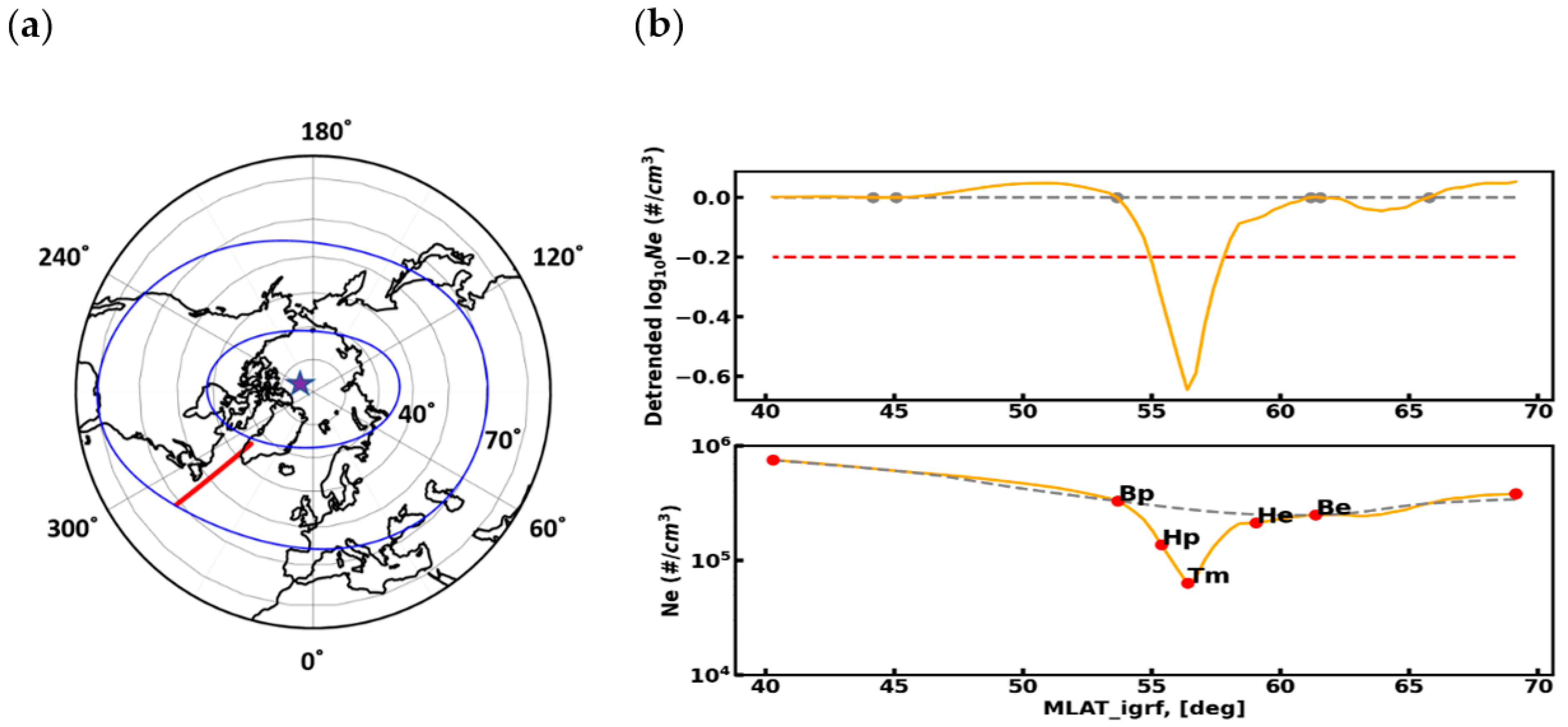
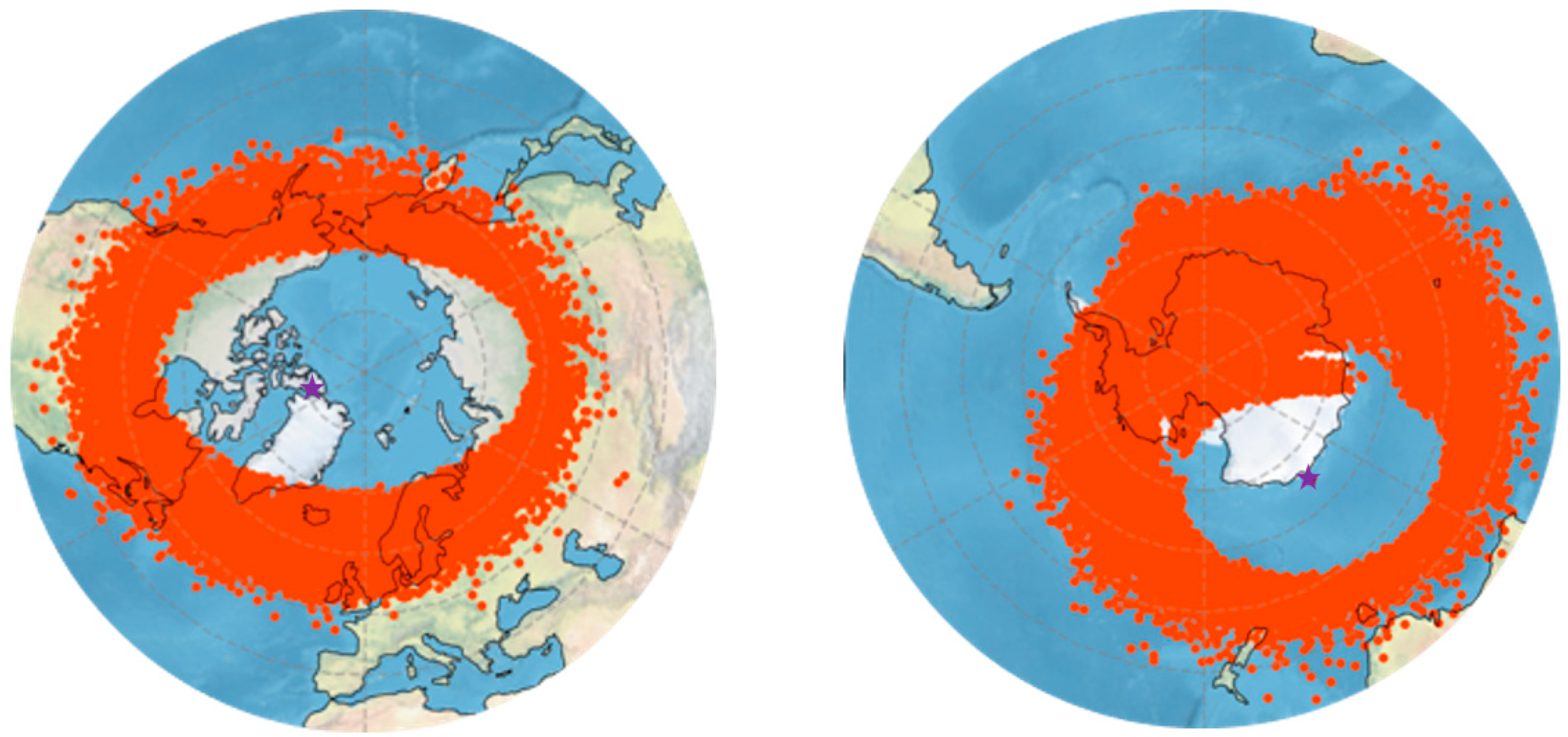
We treated Ne data of one satellite passing from the geomagnetic equator to the pole or vice versa as one Ne profile. As previously mentioned, we only considered Ne profile data in the 40–70° magnetic latitude regions in both hemispheres. Data from other latitude regions (i.e., 40°S−40°N magnetic latitude) were removed from the database. Blue curved lines indicate the MIT search regions in the left plots of Figure 2 for the northern (see top left plot) and southern hemispheres. For geographic to magnetic latitude conversion, we used the International Geomagnetic Reference Field (IGRF) model [25]. The red line curves show the where the GRACE satellites pass over the Northern and Southern hemispheres (see Figure 2, left panel plots).

2.

The background electron density is calculated as a running average of the Ne in a sliding window of 48 data points. The window size is adapted according to a data resolution equivalent to a horizontal distance of ~1800 km. This window size was proven to most optimal. A smaller window size detects some minor irregularities, and a larger window does not properly identify troughs. In Figure 2 (see right panel plots), the background electron density is represented by the black dashed line.

3.

We considered −0.2 detrended log₁₀ (Ne) as a threshold value, so if any Ne profile data values fall below the −0.2 level, the profile is identified as an MIT profile. The trough was detected within the detrended logarithmic electron density. The formula is:

$$lo{g}_{10} \left(Ne\right)-lo{g}_{10} \left(N{e}_{MM}\right),$$

(1)

where $N{e}_{MM}$ is moving mean with a window size of 48 points.

We examined all profiles for negative peaks below the −0.2 level of detrended logarithmic electron density, representing a decrease of about 37% in background electron density. The threshold level was chosen as the most optimal to provide a reliable quality and quantity of detections.

4.

If an MIT occurrence is detected in a profile, the next step is to determine the MIT characteristics. Using the Ne profile data, we determined different points/locations, such as the minimum density location or trough minimum (Tm), the equatorward breakpoint (Be), the poleward breakpoint (Bp), the equatorward half point (He), and the poleward half point (Hp) (see Figure 2). The corresponding definitions are provided later in this manuscript.

5.

The trough identification quality was verified by applying a trough width filter. The threshold of this criterion was established in a range between 1° and 17° [6]. Moreover, in assessing the depth of the trough, the range of electron density was assumed to be between 10³ and 10⁵ cm³ to improve the quality of the detection technique, and Ne values outside this limit were considered outliers. Trough width and depth were calculated using the detected Ne values of trough breakpoints and trough minima.

Figure 2 shows a graphic representation of the MIT detection approach. The left plots (see Figure 2a,c) show examples of satellites passing between 40° and 70° MLAT in the northern and southern hemispheres (red line). The right plots (see bottom panels of Figure 2b,d) show the original Ne variation (see yellow curve) and the background Ne variation along the MLAT (black dashed line). The detected MIT characteristic points are marked in the Ne variation plot. The detrended Ne variation is shown in the upper panels of b and d, where a constant line indicates the threshold level at −0.2 (red dashed line).

The MIT detection approach was applied to all available GRACE KBR Ne profiles, and we detected approximately 44,930 Ne profiles with MIT signatures. Among them, approximately 16,210 profiles were found in the northern hemisphere and approximately 28,720 in the southern hemisphere. The number of detected profiles varies yearly (see Figure 3). The blue-colored bars in Figure 3 show the number of Ne profiles observed during each year from 2002 until 2015 over the northern (see Figure 3a) and southern hemispheres (see Figure 3b). The yellow bar plots show the number of profiles detected with MIT signatures in each hemisphere.

A comparison of the blue and yellow bar plots during the complete period from 2002 to 2015 revealed relatively fewer MIT profiles detected during the solar minimum period of 2007–2010, indicating that the probability of MIT occurrence is related to the solar cycle variation.

As previously mentioned, if an MIT occurrence was detected, the locations of the trough minimum (Tm), the equatorward and poleward breakpoints (Be and Bp), and the equatorward and poleward half points (He and Hp) were determined. The breakpoints were determined as the intersection points of the Ne profile and the background density. Then, the trough width and trough depth were determined as shown in Figure 4. The trough width is defined as the spatial distance between the breakpoints (Be and Bp), whereas the trough depth is defined as the electron density difference between the value of the breakpoint and the trough minimum point.

3. Results and Discussion

As mentioned in the previous section, approximately 45,000 Ne profiles were detected with MIT signatures. Thus, we obtained a database of MIT parameters, such as trough minimum, trough width, and trough depth. The occurrences of MIT parameters are statistically analyzed in this section. The parameters were analyzed as functions of different space weather indices, for instance, solar radio flux index F10.7; solar wind (SW) plasma speed; flow pressure; interplanetary magnetic field components Bx, Bz, and By; SYM–H; and Hp30. Additionally, the dependency of MIT parameters on different geophysical conditions, such as geographic/magnetic location, magnetic local time, and seasons, were analyzed.

3.1. Geographical Distribution

Figure 5 shows the location of the trough minimum on global maps separately for the northern and southern hemispheres. The trough minimum location is distributed around the magnetic pole (marked by a magenta star sign), forming an approximately elliptical shape.

3.2. Solar Cycle Dependence

Solar radio flux index F10.7 is used here as a proxy for solar activity conditions. The percentage occurrence of the MIT (i.e., (no. of detected MIT profiles)/(total no. of profiles) × 100%) was computed and plotted for each year, as shown in Figure 6. The blue and yellow bars indicate the MIT percentage occurrence for the northern and southern hemispheres, respectively. The red line curve shows the yearly mean variation of F10.7 (see right scale). Comparing the MIT percentage occurrence and F10.7 plots reveals a positive correlation between these two parameters. We found that the occurrence rate of the MIT increases with increased F10.7 values and decreases with decreased F10.7 values. The occurrence rate is approximately 5–20% higher in the southern hemisphere compared to the northern hemisphere throughout the year. The correlation coefficient for F10.7 and MIT percentage occurrence in the southern hemisphere is 0.73, and that in the northern hemisphere is 0.67.

Figure 7 compares the trough means and minima positions in MLAT and F10.7 for 2002–2015. The yearly average of F10.7 is separately plotted for the northern and southern hemispheres, considering only days for which MIT was detected. Because the MIT is not always simultaneously detected in both hemispheres, the F10.7 average plots do not precisely coincide. Figure 7 shows that the trough minimum location moves poleward during low-solar-activity years (2007–2010) and equatorward during high-solar-activity years in both hemispheres. In the northern hemisphere, the dependence on the solar cycle is more pronounced. The results are in agreement with those reported by Karpachev et al. (2016) [26]. The trough minimum is observed at approximately 2–4 degrees higher latitude in the northern hemisphere compared to the southern hemisphere.

The mean and standard deviation (STD) values of trough depth and width were computed for equal-sized F10.7 bins. Figure 8 shows the mean variation in trough depth and width as a function of the F10.7 index. The corresponding STD values are plotted as error bars. We found a clear dependence of the trough depth on the F10.7. The left panel plots show that the trough depth increases with increased F10.7 until it reaches saturation at approximately 200 flux units. A positive correlation between the trough depth and F10.7 increase was also found by Ishida et al. (2014), which is caused by dissociative recombination as a result of a high ion temperature correlated with increasing F10.7 levels [15]. The right panel shows that the mean trough width remains almost constant with the increase in the F10.7 and is larger for the northern hemisphere than the southern hemisphere.

3.3. Seasonal Variation

In this section, we address the dependence of the MIT parameters on seasonal variation. Figure 9 shows the percentage occurrence of the MIT during each month separately in the northern (left plot) and southern hemispheres. The northern plot shows that the MIT occurs more often in winter months (Nov–Feb) and equinoxes than in summer (May–Aug). The southern plot shows a similar (i.e., opposite, as seasons are opposite) trend, although the seasonal dependence is less pronounced. The high MIT occurrence during equinoxes may be linked to the increased auroral activity around the equinoctial months. Increased auroral activity facilitates the buildup of the main trough′s poleward wall, leading to easier identification of trough signatures around equinoxes.

Furthermore, during geomagnetic activities, the ionospheric convection flows increase, and as a result, due to the frictional heating mechanism, more troughs eventually form [18]. Seasonal fluctuations are more pronounced in the northern hemisphere than in the southern hemisphere, which indicates hemispheric asymmetry. This could be related to the offset of the magnetic and geographic poles [18].

Figure 10 shows the MIT distribution during December solstice (Nov–Feb), June solstice (May–Aug), and the equinoxes (Mar, Apr, Sep, Oct) over the northern (see top panel) and southern hemispheres. The scatter plots show the MIT minimum positions on global maps. An ellipse approximates the mean position of the MIT minimum for each season. The mean values were first determined by binning trough location with one-degree geographical latitudinal and longitudinal resolution; the mean values were then fitted to the ellipses. We used a similar algorithm to fit the ellipsoids to data described by Kamal et al. [27].

We further investigated the spatial distribution of the MIT minimum depending on the season (see

Table 2. Mean position of the trough minimum during December solstice, June solstice, and the equinoxes. The corresponding standard deviations are given after the ± sign.

	Northern Hemisphere	Southern Hemisphere
December solstice	60.59 ± 4.05	−55.8 ± 6.02
Equinoxes	60.23 ± 4.14	−55.72 ± 6.21
June solstice	59.08 ± 4.09	−56.8 ± 5.97

). We computed the mean position of the MIT minimum and corresponding STD values during the December solstice, June solstice, and the equinoxes. The statistical estimates are presented in Table 2 (STD values are given after ± sign). We found that the mean trough minimum position varies slightly depending on the season. Compared to the values during equinoxes, the mean trough minimum moves equatorward during local summer (June solstice for NH and December solstice for SH). In contrast, during local winter (December solstice for NH and June solstice for SH), the mean trough minimum moves poleward. The standard deviation values are lower for the NH than for the SH.

In order to determine the seasonal variation in Tm, width, and depth, their monthly mean and STDs were computed. The monthly mean variations in Tm, width, and depth are plotted in Figure 11. The corresponding STDs are plotted as error bars. The plot for the southern hemisphere (blue line) shows that the MIT is deeper during the winter months (May-Aug) than during the summer months. The plot for the northern hemisphere (yellow line) shows a similar trend, although the seasonal dependence is less pronounced. The Tm variation shows that during winter months, the Tm position is located at slightly higher latitudes compared to summer months (see first panel). In the southern hemisphere, the MIT is located at a higher latitude in the summer period. The trough width varies from 8 to 10 degrees in the northern hemisphere, and in the southern hemisphere, the trough width is smaller, and in the range of 5 to 7 degrees [18]. The trough width broadens in wintertime, with an opposite correlation in the southern hemisphere. This could be caused by the poleward extension of the nighttime ionosphere in winter due to the axial rotation tilt of Earth [18].

The left plot shows the variation in the monthly mean trough minimum position as a function of months. The northern hemisphere plot illustrates that the trough minimum shifts poleward during winter months and equatorward during summer months. In the southern hemisphere, the trough variations exhibit opposite behavior. These results are in agreement with the results presented in Table 2.

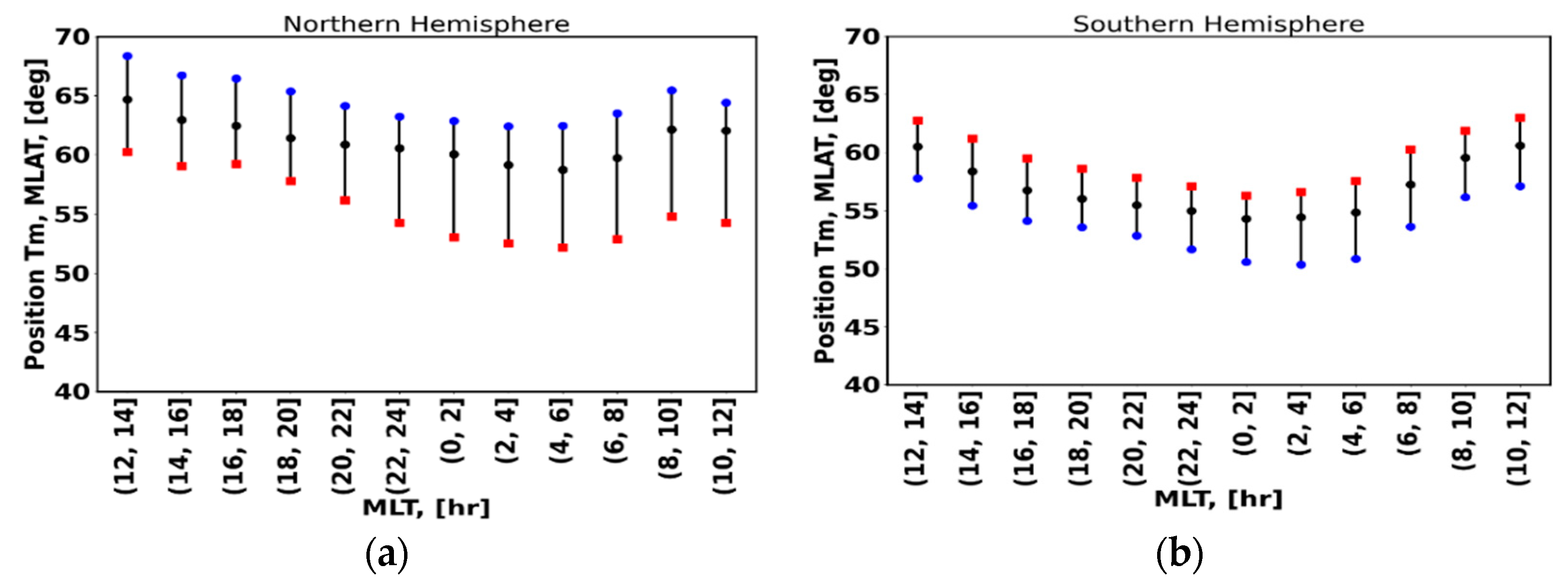
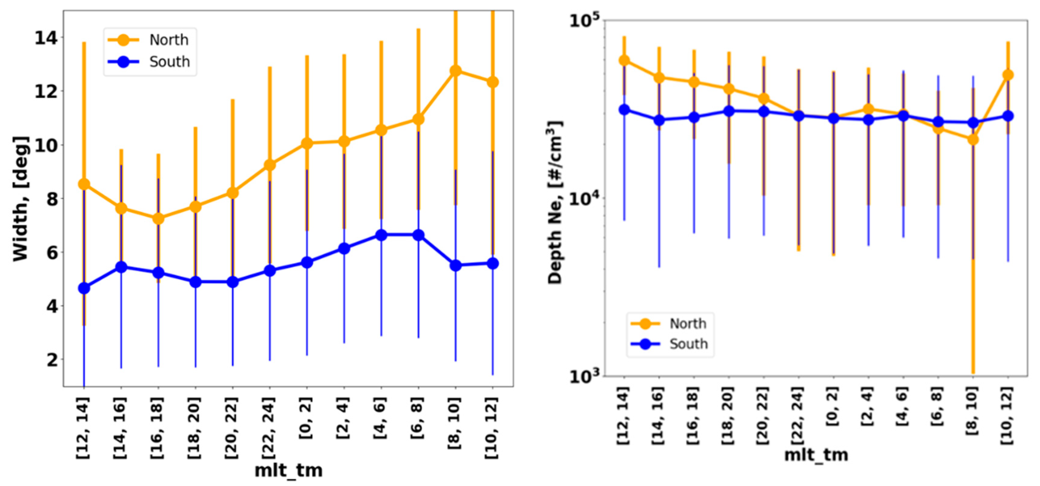
3.4. Diurnal Variation

Figure 12 illustrates a polar view of the trough occurrence depending on the magnetic local time (MLT) and the magnetic latitude for the northern (Figure 12a–c) and southern (Figure 12d–f) hemispheres. The trough minimum position was binned with a resolution of 2° latitude ×1 h. The percentage occurrence was calculated by dividing the trough minimum position in each sector by the total number of available profiles in the sector and multiplying by 100. Figure 12 shows that the trough polar plot for each season expands in latitude from 60 to 50 MLAT and elongates from dusk to dawn. This occurs more often at night and in the morning. Rodger et al. (1992) suggested that a boundary between the dusk and morning trough should exist due to different flow regimes [9]. For the northern hemisphere, the trough occurs more often during the December solstice and equinoxes. For the southern hemisphere, it occurs more often during equinoxes and the June solstice, as discussed in the previous section.

Figure 13 shows the variation in mean trough minimum position (marked by black dots) as a function of magnetic local time (MLT). The corresponding mean trough widths are plotted as error bars. The trough width is bounded by trough equatorward and poleward breakpoints (see Figure 13).

For the northern hemisphere, the mean trough widths are smaller in the poleward direction, indicating a sharp slope or high gradient. The trough widths are comparatively larger in the equatorward direction, indicating a less sharp slope. A similar trend is observed in the southern hemisphere, although the widths are comparatively smaller in both directions.

Diurnal variations in the trough width and depth are represented in Figure 14.

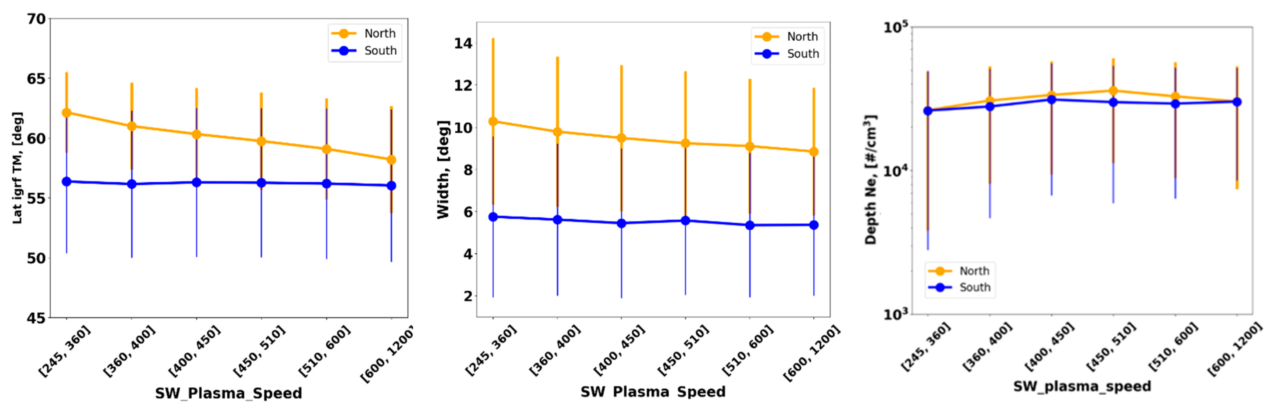
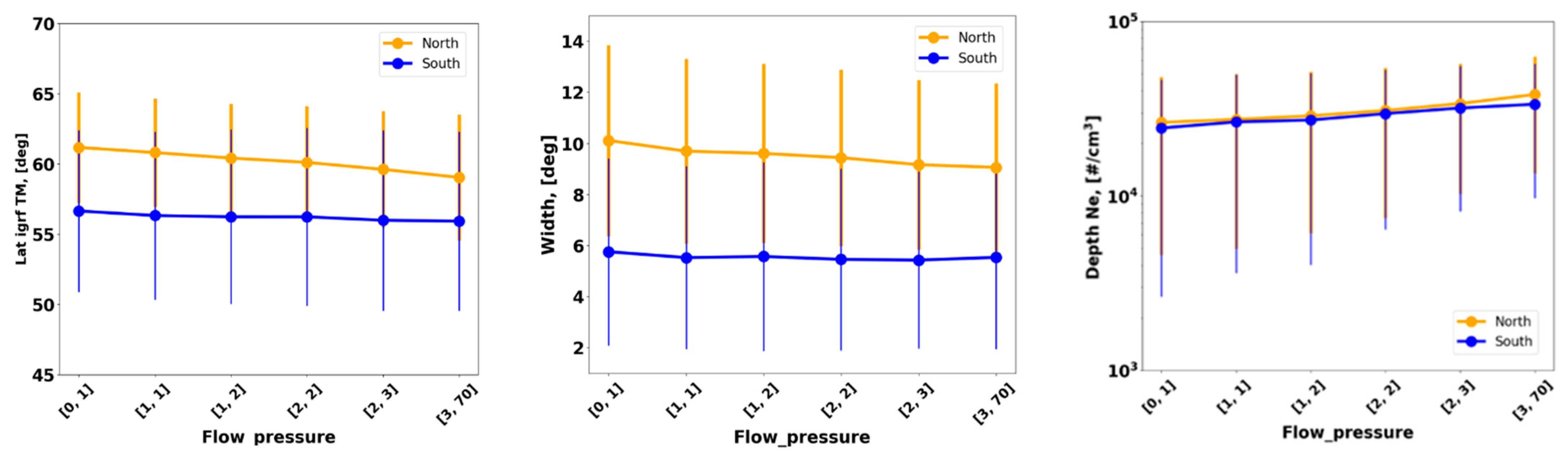
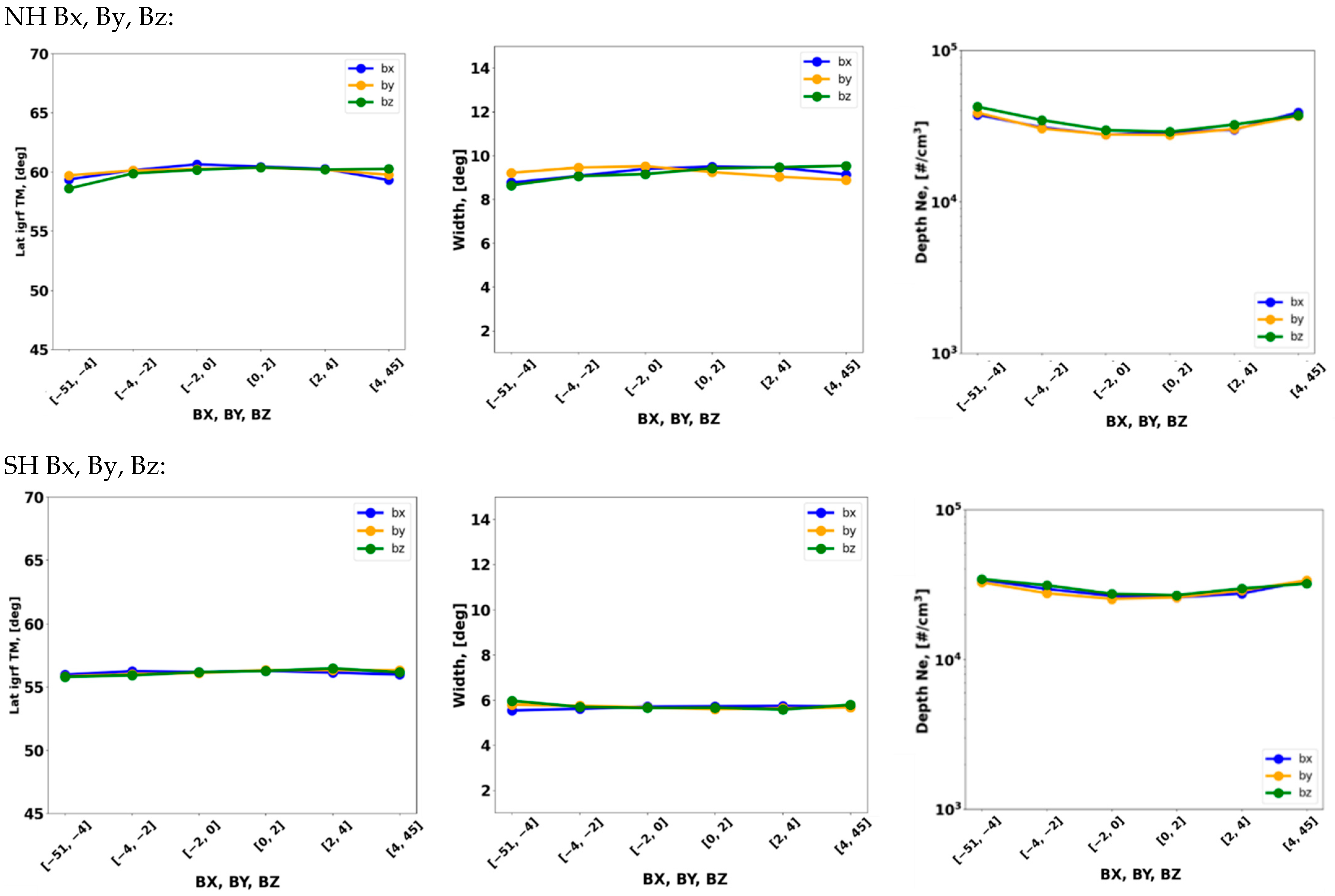
3.5. Dependence on Solar Wind; Flow Pressure; and IMF Bx, Bz, and By Components

We examined the correlation between the main trough parameters and solar wind plasma speed (see Figure 15); flow pressure (see Figure 16); and IMF Bx, Bz, and By components (see Figure 17). The dependence on solar wind and trough minimum location shows a negative correlation in the northern hemisphere. A negative correlation between the MIT latitude and solar wind speed was also reported by He et al. (2011) [14]. The trough width decreases with increased solar wind speed, and the southern hemisphere shows no visible correlation with solar wind.

Correlation with flow pressure is presented in Figure 16. With increasing flow pressure, the trough moves slightly to lower latitudes and becomes narrower and deeper in both hemispheres.

Figure 17 shows the variation in the trough minimum position relative to the Bx, By, and Bz components. The variation in the trough parameters is very low, and all the IMF components show a similar trend.

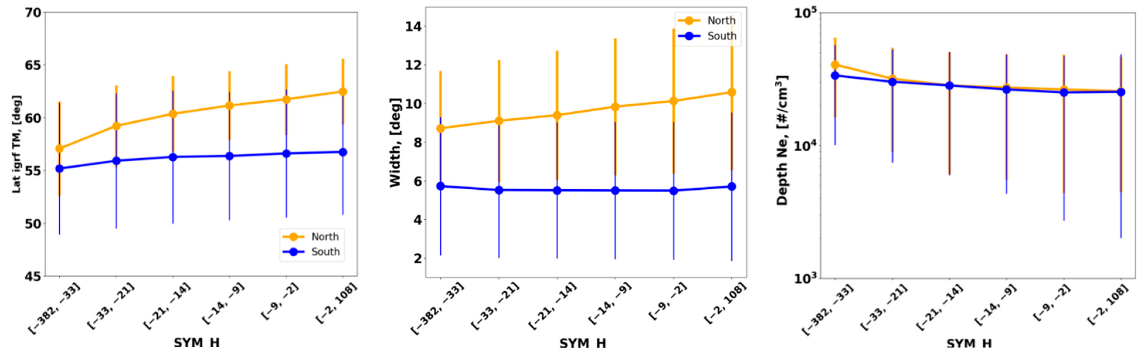
3.6. Dependence on the SYM-H Index

The SYM-H index is similar to the Dst-index but has a different time resolution and method to determine the base value. The temporal resolution of the SYM-H index is 1 min. Wanliss et al. [28] found that the SYM-H index is accurate and should be used as a replacement in future studies. Figure 18 shows the dependence of Tm, width, and depth according to SYM-H index. The SYM-H index shows a clear correlation with the main trough parameters, and in the northern hemisphere, this dependence is more prominent than in the southern hemisphere. With a decreasing SYM-H index, the trough moves equatorward. The trough becomes narrower and deeper with a decreasing SYM-H index. Our results confirm the previous findings by Yang et al. (2016) [19], who showed that the trough dynamics differ depending on the magnetic storm category and that the shift in the position of the trough in the northern and southern hemispheres during magnetic storms is symmetrical.

3.7. Dependence on the Hp30 Index

The Hp30 index is a high-cadence index that is similar to the Kp index, although its resolution is 30 min [25]. The Kp index has been used in several MIT model approaches, for example, by Deminov and Shubin (2018) [29] and Karpachev et al. (2016) [26]. We examined the dependence on a high-cadence Hp30 index of trough minimum location, width, and depth. The results are presented in Figure 19. The trough moves equatorward with an increasing Hp30 index. In the northern hemisphere, this dependence is more prominent than in the southern hemisphere. Furthermore, the northern hemisphere has pronounced dependence on the Hp30 index for trough width. The trough widens with a decreasing Hp30 index. The depth has an opposite dependence, i.e., trough deepens with an increasing Hp30 index.

The observed correlation between the geomagnetic activity level and the trough position is in agreement with results of previous studies [9,16]. This relationship can be partly explained by storm time subauroral polarization streams (SAPS) or subauroral ion drift (SAID) flow channels, which also clearly depend on geomagnetic activity levels [18].

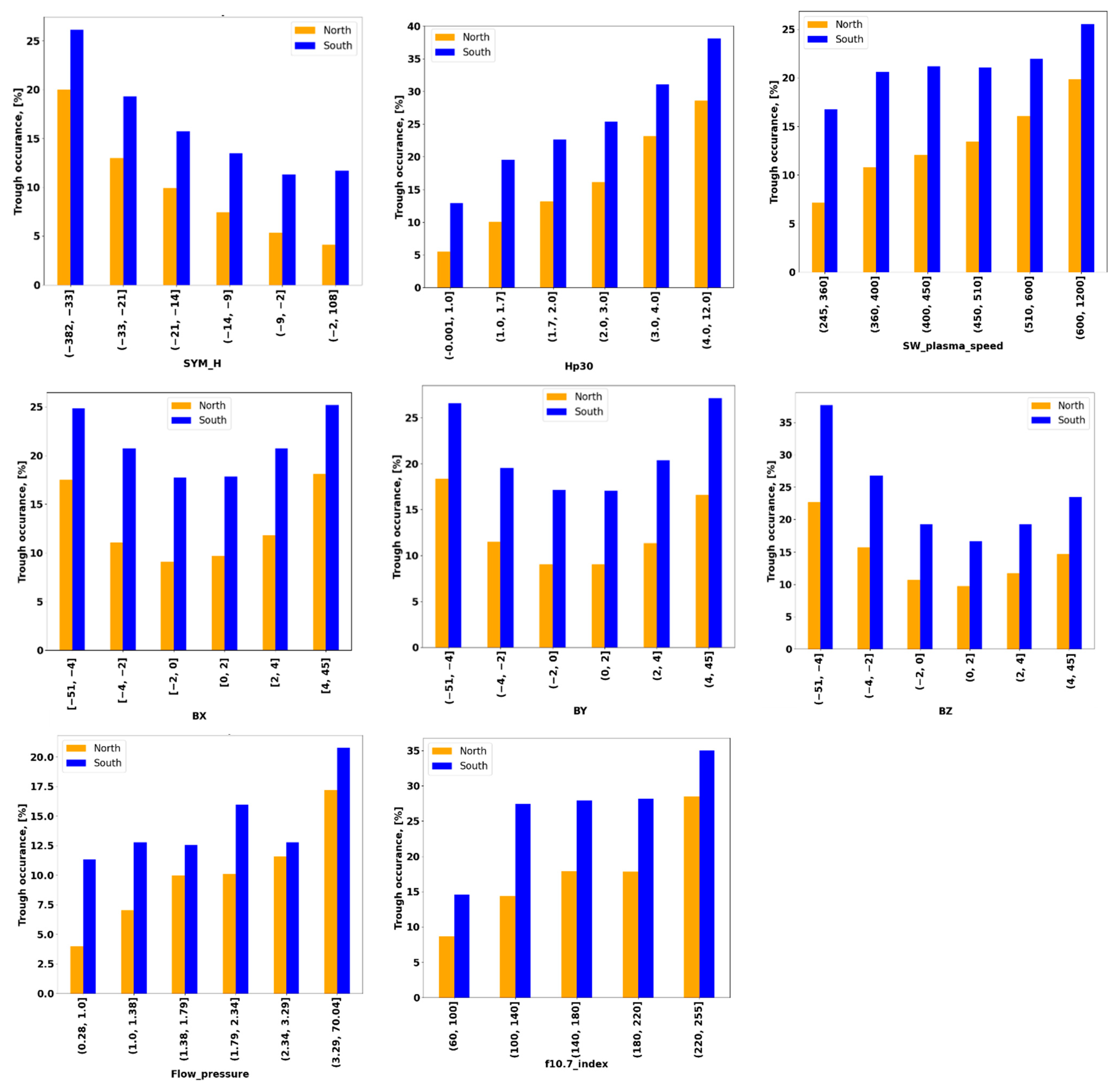
3.8. Trough Occurrence Dependence on Space Weather Indices

We analyzed the occurrence of the trough relative to space weather indices. The results are presented in Figure 20. The Hp30 index shows that the trough occurred more often with increasing geomagnetic activity in both hemispheres. The trough occurrence increases with decreasing SYM-H index (which indicates storm occurrence). Solar wind plasma speed has a slight influence on trough occurrence, increasing with increased wind speed. Flow pressure also correlates with MIT formation. With increased flow pressure, the trough occurrence increases. The influence of IMF on the MIT was investigated by Rodger et al. (1992) [9] and by Voiculescu et al. (2006) [16]. The Bz component has the most significant effect on magnetosphere–ionosphere coupling; consequently, it should have the most significant impact on the trough [16]. As shown in Figure 20, the Bz component has the greatest influence on the occurrence percentage value of the MIT.

4. Conclusions

In this paper, we presented a statistical evaluation of the main ionospheric trough in the northern and southern hemispheres from 2002 to 2015 using KBR electron density measurements from the GRACE satellite mission. Our database of MIT profiles contains 16,212 profiles for the northern hemisphere and 28,721 profiles for the southern hemisphere. The evaluation was performed using MIT parameters, such as the trough minimum position, width, depth, and occurrence in relation to geographical location, solar cycle, seasons, magnetic local time, and space weather indices.

We obtained comprehensive results, showing that:

• The trough minimum location is distributed around the magnetic north and south poles, forming an ellipsoid;
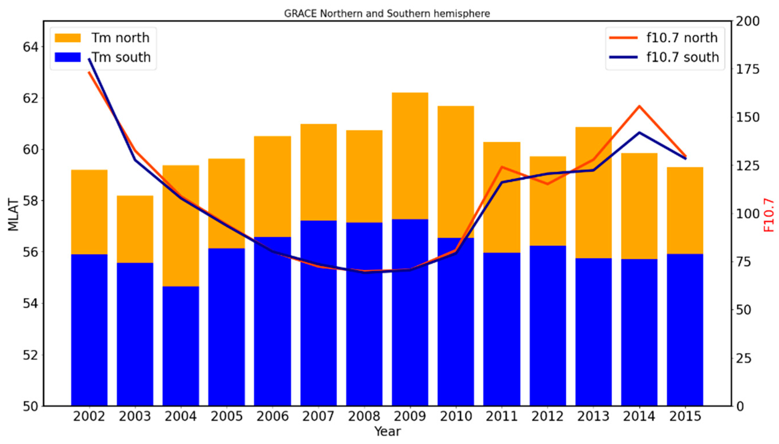
• The trough location moves poleward under low-solar-activity conditions and equatorward under high-solar-activity conditions in both hemispheres;
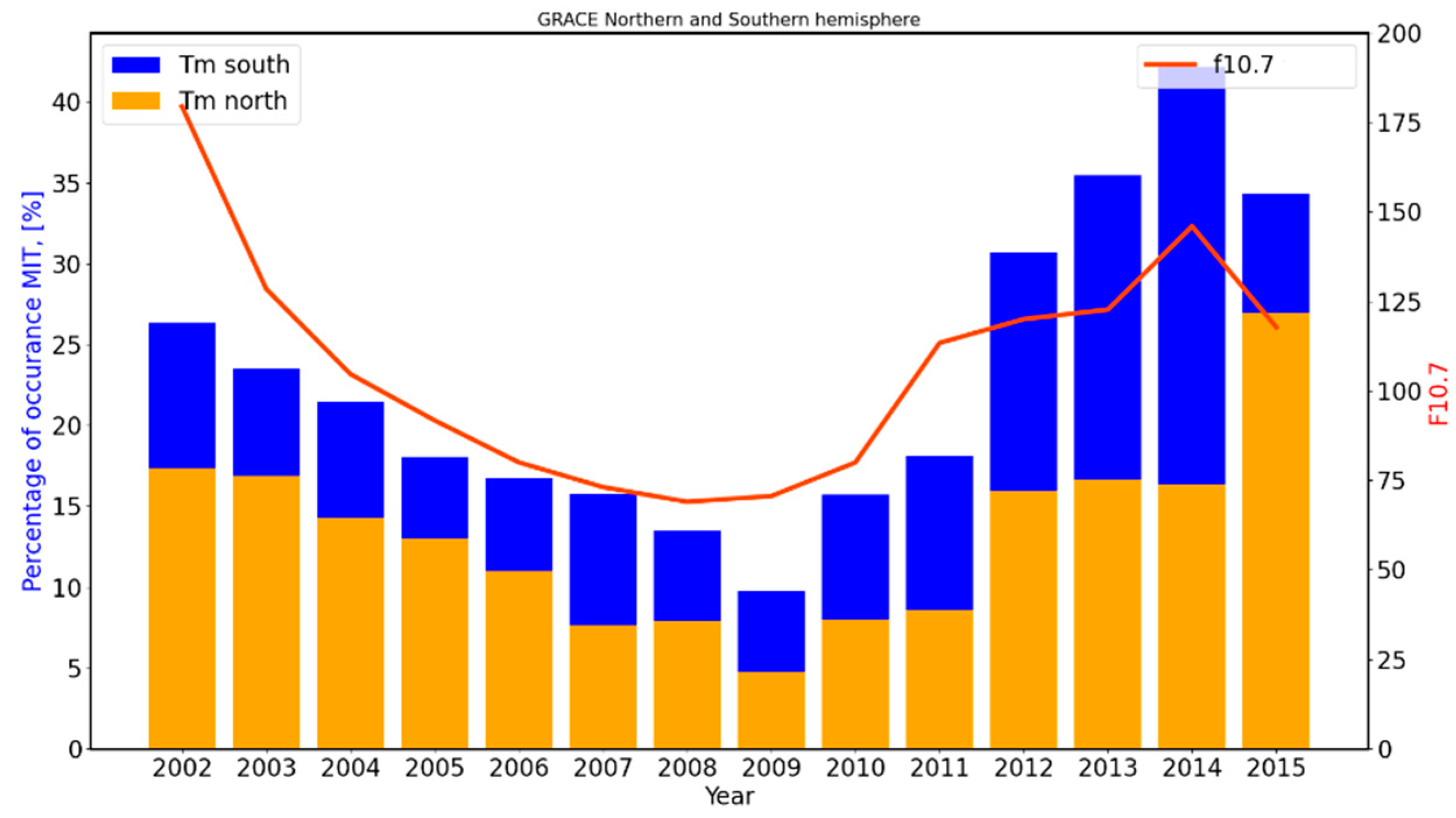
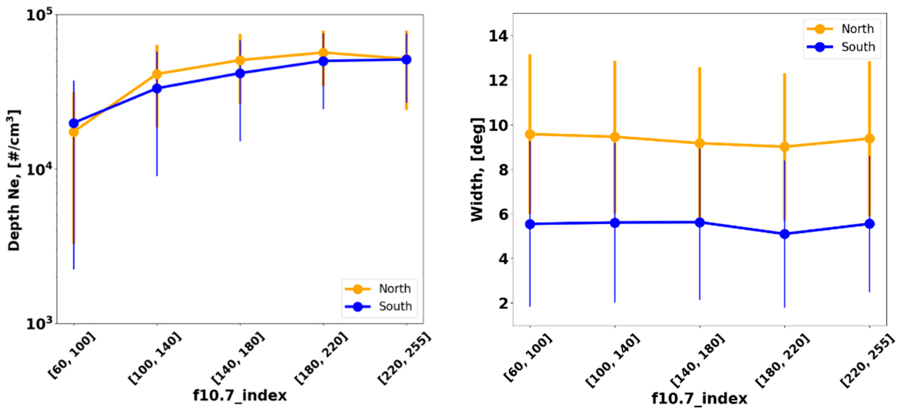
• The occurrence probability of the MIT depends on solar activity. The occurrence of the trough increases with increased F10.7 values. Furthermore, the position of the MIT changes depending on solar activity, moving poleward under low-solar-activity conditions and equatorward under high-solar-activity conditions in both hemispheres; however, this dependency is more prominent in the northern hemisphere than in the southern hemisphere. The trough depth increases with increased in F10.7 values;
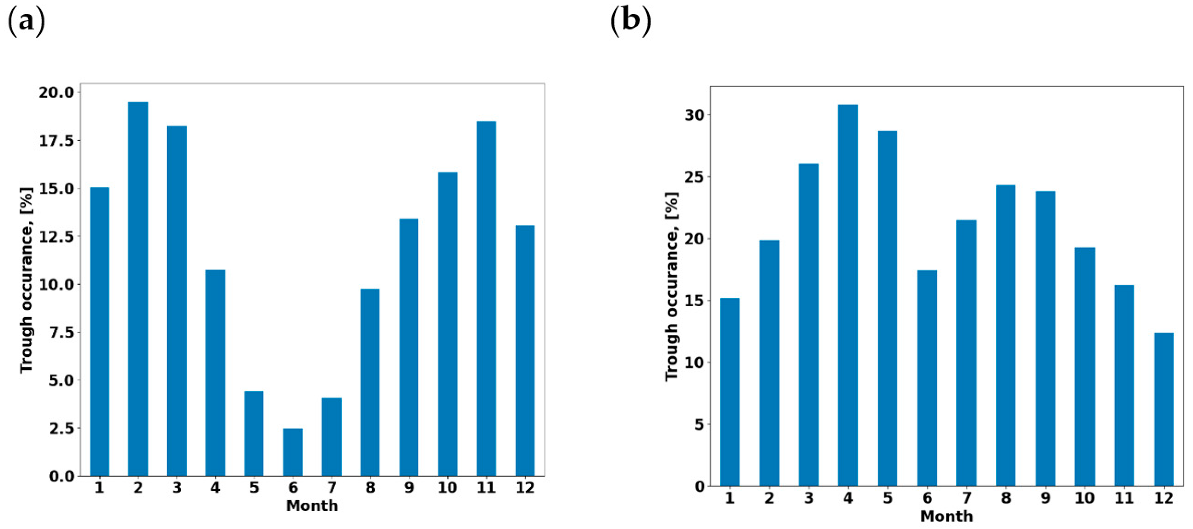
• Seasonal dependency of MIT is more pronounced in the northern hemisphere than in the southern hemisphere. The MIT occurs more often in winter months (Nov–Feb) and equinoxes than in summer (May–Aug) months. The trough is deeper during local winter months in the southern hemisphere compared to summer months, whereas the trough width exhibits opposite behavior in the northern hemisphere. The MIT width varies from 8 to 10° in the northern hemisphere and from 5 to 7° in the southern hemisphere. The trough minimum moves poleward during winter months and equatorward during summer months;
• The mean trough widths are smaller in the poleward direction, indicating a sharper slope. The mean trough width is larger in the equatorward direction, showing a less sharp slope;
• The MIT shows a clear correlation with the SYM-H index. In the northern hemisphere, this dependence is more prominent than in the southern hemisphere. With decreasing SYM-H index values (indicating storm conditions), the trough moves equatorward narrows and deepens with decreasing SYM-H index values;
• A comparison with the high-cadence Hp30 index shows a correlation with the MIT location, moving equatorward with increased HP30 values. In the northern hemisphere, this dependence is more prominent than in the southern hemisphere. Furthermore, the trough widens with decreasing Hp30 index values, whereas depth shows an opposite dependence, i.e., the trough deepens increasing Hp30 index values;
• Trough occurrences increase with decreasing geomagnetic disturbance index SYM-H values;
• MIT occurrences positively correlate with Hp30, f10.7, flow pressure, and solar wind plasma speed indices.

Our study confirms previous MIT investigations and contributes new results with respect to the dependence of the MIT’s on geophysical conditions. In this study, we presented, for the first time, the ellipse distribution for the northern and southern hemispheres of the mean position of the trough minimum in three seasons. We also elucidated the dependence of the MIT on the flow pressure index and high-resolution indices, such as the SYM-H and Hp30 indices. Moreover, the dependence of MIT occurrence on the space weather indices was investigated. The obtained information with respect to MIT dependency and occurrence probability can be used for MIT model validation, as well as for the development of new MIT models.

GRACE data were recently reprocessed, now covering the entire mission, and data of the follow-on mission, GRACE-FollowOn, are also available (https://earth.esa.int/eogateway/news/new-swarm-tiro-dataset-released, accessed on 27 June 2022), offering perspectives of increased climatology of the MIT for future works.

References

1. Muldrew, D.B. F-Layer Ionization Troughs Deduced from Alouette Data. J. Geophys. Res. 1965, 70, 2635–2650. [Google Scholar] [CrossRef]
2. Bilitza, D. IRI the International Standard for the Ionosphere. Adv. Radio Sci. 2018, 16, 1–11. [Google Scholar] [CrossRef]
3. OS SIS ICD. European GNSS Galileo Open Service Signal in Space Interface Control Document; SISICD-2006, Issue 1.1; European Space Agency: Paris, France, 2010. [Google Scholar]
4. Nava, B.; Coïsson, P.; Radicella, S.M. A New Version of the NeQuick Ionosphere Electron Density Model. J. Atmos. Sol.-Terr. Phys. 2008, 70, 1856–1862. [Google Scholar] [CrossRef]
5. Hoque, M.M.; Jakowski, N.; Orús-Pérez, R. Fast Ionospheric Correction Using Galileo Az Coefficients and the NTCM Model. GPS Solut. 2019, 23, 41. [Google Scholar] [CrossRef]
6. Karpachev, A. The Dependence of the Main Ionospheric Trough Shape on Longitude, Altitude, Season, Local Time, and Solar and Magnetic Activity. Geomagn. Aeron. 2003, 43, 239–251. [Google Scholar]
7. Liu, Y.; Xiong, C. Morphology Evolution of the Midlatitude Ionospheric Trough in Nighttime under Geomagnetic Quiet Conditions. J. Geophys. Res. Space Phys. 2020, 125, e2019JA027361. [Google Scholar] [CrossRef]
8. Rodger, A. The Mid-Latitude Trough—Revisited. In Midlatitude Ionospheric Dynamics and Disturbances; American Geophysical Union (AGU): Washington, DC, USA, 2008; pp. 25–33. ISBN 978-1-118-66655-5. [Google Scholar]
9. Rodger, A.S.; Moffett, R.J.; Quegan, S. The Role of Ion Drift in the Formation of Ionisation Troughs in the Mid- and High-Latitude Ionosphere—A Review. J. Atmos. Terr. Phys. 1992, 54, 1–30. [Google Scholar] [CrossRef]
10. Zou, S.; Moldwin, M.B.; Coster, A.; Lyons, L.R.; Nicolls, M.J. GPS TEC Observations of Dynamics of the Mid-Latitude Trough during Substorms. Geophys. Res. Lett. 2011, 38, L14109. [Google Scholar] [CrossRef]
11. Heilig, B.; Stolle, C.; Kervalishvili, G.; Rauberg, J.; Miyoshi, Y.; Tsuchiya, F.; Kumamoto, A.; Kasahara, Y.; Shoji, M.; Nakamura, S.; et al. Relation of the Plasmapause to the Midlatitude Ionospheric Trough, the Sub-Auroral Temperature Enhancement and the Distribution of Small-Scale Field Aligned Currents as Observed in the Magnetosphere by THEMIS, RBSP, and Arase, and in the Topside Ionosphere by Swarm. J. Geophys. Res. Space Phys. 2022, 127, e2021JA029646. [Google Scholar] [CrossRef]
12. Davies, K. Ionospheric Radio; IET Digital Library: London, UK, 1990; ISBN 978-1-84919-387-0. [Google Scholar]
13. Werner, S.; Prölss, G.W. The Position of the Ionospheric Trough as a Function of Local Time and Magnetic Activity. Adv. Space Res. 1997, 20, 1717–1722. [Google Scholar] [CrossRef]
14. He, M.; Liu, L.; Wan, W.; Zhao, B. A Study on the Nighttime Midlatitude Ionospheric Trough. J. Geophys. Res. Space Phys. 2011, 116. [Google Scholar] [CrossRef]
15. Ishida, T.; Ogawa, Y.; Kadokura, A.; Hiraki, Y.; Häggström, I. Seasonal Variation and Solar Activity Dependence of the Quiet-Time Ionospheric Trough. J. Geophys. Res. Space Phys. 2014, 119, 6774–6783. [Google Scholar] [CrossRef]
16. Voiculescu, M.; Virtanen, I.; Nygrén, T. The F-Region Trough: Seasonal Morphology and Relation to Interplanetary Magnetic Field. Ann. Geophys. 2006, 24, 173–185. [Google Scholar] [CrossRef]
17. Yang, N.; Le, H.; Liu, L. Statistical Analysis of Ionospheric Mid-Latitude Trough over the Northern Hemisphere Derived from GPS Total Electron Content Data. Earth Planets Space 2015, 67, 196. [Google Scholar] [CrossRef]
18. Aa, E.; Zou, S.; Erickson, P.J.; Zhang, S.-R.; Liu, S. Statistical Analysis of the Main Ionospheric Trough Using Swarm in Situ Measurements. J. Geophys. Res. Space Phys. 2020, 125, e2019JA027583. [Google Scholar] [CrossRef]
19. Yang, N.; Le, H.; Liu, L. Statistical Analysis of the Mid-Latitude Trough Position during Different Categories of Magnetic Storms and Different Storm Intensities. Earth Planets Space 2016, 68, 171. [Google Scholar] [CrossRef]
20. Xiong, C.; Lühr, H.; Stolle, C. GRACE Electron Density Derived from the K-Band Ranging System (KBR); GFZ Data Services: Potsdam, Germany, 2021. [Google Scholar] [CrossRef]
21. Xiong, C.; Lühr, H.; Ma, S.; Schlegel, K. Validation of GRACE Electron Densities by Incoherent Scatter Radar Data and Estimation of Plasma Scale Height in the Topside Ionosphere. Adv. Space Res. 2015, 55, 2048–2057. [Google Scholar] [CrossRef]
22. OMNIWeb Data Explorer. Available online: https://omniweb.gsfc.nasa.gov/form/dx1.html (accessed on 22 February 2022).
23. OMNIWeb: High Resolution OMNI. Available online: https://omniweb.gsfc.nasa.gov/form/omni_min.html (accessed on 22 February 2022).
24. Yamazaki, Y.; Matzka, J.; Stolle, C.; Kervalishvili, G.; Rauberg, J.; Bronkalla, O.; Morschhauser, A.; Bruinsma, S.; Shprits, Y.Y.; Jackson, D.R. Geomagnetic Activity Index Hpo. Geophys. Res. Lett. 2022, 49. [Google Scholar] [CrossRef]
25. Alken, P.; Thébault, E.; Beggan, C.D.; Amit, H.; Aubert, J.; Baerenzung, J.; Bondar, T.N.; Brown, W.J.; Califf, S.; Chambodut, A.; et al. International Geomagnetic Reference Field: The Thirteenth Generation. Earth Planets Space 2021, 73, 49. [Google Scholar] [CrossRef]
26. Karpachev, A.; Klimenko, M.; Klimenko, V.; Poustovalova, L. Empirical Model of the Main Ionospheric Trough for the Nighttime Winter Conditions. J. Atmos. Sol.-Terr. Phys. 2016, 146, 149–159. [Google Scholar] [CrossRef]
27. Kamal, S.; Jakowski, N.; Hoque, M.M.; Wickert, J. E Layer Dominated Ionosphere Occurrences as a Function of Geophysical and Space Weather Conditions. Remote Sens. 2020, 12, 4109. [Google Scholar] [CrossRef]
28. Wanliss, J.A.; Showalter, K.M. High-Resolution Global Storm Index: Dst versus SYM-H. J. Geophys. Res. Space Phys. 2006, 111. [Google Scholar] [CrossRef]
29. Deminov, M.G.; Shubin, V.N. Empirical Model of the Location of the Main Ionospheric Trough. Geomagn. Aeron. 2018, 58, 348–355. [Google Scholar] [CrossRef]
Figure 1. Evolution of the orbital altitude during the GRACE mission.
Remotesensing 14 04384 g001
Figure 2. Examples of the GRACE trajectory over the northern (a) and southern (c) hemispheres on 14 April 2002 between 40° and 70° magnetic latitudes. Concentric circles are plotted in 10° intervals. The blue lines correspond to magnetic latitudes 40° and 70°. The red line is the footprint of the satellite path. The magnetic pole is marked with a star. Corresponding Ne profiles with detected trough minimum position and trough characteristic points for the northern (b) and southern (d) hemispheres (see below plots). Detrended logs of Ne are represented in upper plots for the northern (b) and southern (d) hemispheres. The gray dashed line represents the Ne running average. The yellow line is the Ne profile, and the red dashed line shows the threshold for trough detection.
Remotesensing 14 04384 g002aRemotesensing 14 04384 g002b
Figure 3. Number of total and detected MIT profiles for each year in the northern hemisphere (a) and the southern hemisphere (b).
Remotesensing 14 04384 g003
Figure 4. Schematic diagram of the mid-latitude trough characteristic points.
Remotesensing 14 04384 g004
Figure 5. Polar view of geographic locations of trough minimum locations (red dots) for the northern (left plot) and southern (right plot) hemispheres. Purple stars show the locations of the geomagnetic pole for each hemisphere.
Remotesensing 14 04384 g005
Figure 6. Percentage of occurrence of MIT each year in relation to the F10.7 index.
Remotesensing 14 04384 g006
Figure 7. Solar cycle variation in trough minimum location from 2002 to 2015 for the northern and southern hemispheres.
Remotesensing 14 04384 g007
Figure 8. Variation in depth and width of the mid-latitude trough due to the F10.7 index in the northern and southern hemispheres.
Remotesensing 14 04384 g008
Figure 9. Seasonal variation in the MIT occurrence rate for the northern and southern hemispheres. (a) MIT monthly variation in the northern hemisphere; (b) MIT monthly variation in the southern hemisphere.
Remotesensing 14 04384 g009
Figure 10. Ellipse distribution for the northern (ac) and southern (df) hemispheres of the mean position of the trough minimum in three seasons: December solstice (blue color), June solstice (pink color), and equinoxes (green color). Red points in each hemisphere represents the detected trough minimum location. The dark red star shows the locations of the geomagnetic pole for each hemisphere.
Remotesensing 14 04384 g010
Figure 11. Monthly variation in location, depth, and width of the mid-latitude trough for the northern and southern hemispheres.
Remotesensing 14 04384 g011
Figure 12. Polar view of the northern (ac) and southern (df) hemisphere trough occurrence rates in the magnetic local time and magnetic latitude for three seasons: December solstice, June solstice, and equinoxes.
Remotesensing 14 04384 g012
Figure 13. Diurnal variation in trough position for the northern (a) and southern (b) hemispheres as a function of the magnetic local time.
Remotesensing 14 04384 g013
Figure 14. Diurnal variation in trough width and depth for the northern and southern hemispheres as a function of the magnetic local time.
Remotesensing 14 04384 g014
Figure 15. Solar speed dependence of the trough minimum position, trough width, and trough depth for the northern and southern hemispheres.
Remotesensing 14 04384 g015
Figure 16. Flow pressure dependence of the trough minimum position, trough width, and trough depth for the northern and southern hemispheres.
Remotesensing 14 04384 g016
Figure 17. Bx (blue), By (orange), and Bz (green) component dependence of the trough minimum position, trough width, and trough depth for the northern and southern hemispheres.
Remotesensing 14 04384 g017
Figure 18. SYM-H index dependence of the trough minimum position, trough width, and depth for the northern and southern hemispheres.
Remotesensing 14 04384 g018
Figure 19. Hp30 index dependence of the trough minimum position, trough width, and trough depth for the northern and southern hemispheres.
Remotesensing 14 04384 g019
Figure 20. The occurrence of the trough depending on space weather indices for the northern and southern hemispheres.
Remotesensing 14 04384 g020