Assessment of FY-2G, FY-4A, and Himawari-8 Atmospheric Motion Vectors over Southeast Asia and Their Assimilating Impact on the Forecasts of Tropical Cyclone PABUK

Abstract

The spatial coverage of atmospheric motion vectors (AMVs) over Southeast Asia (SEA) is mainly covered by the Himawari-8 (HIMA-8) and FengYun-2 (FY-2) series satellites in the Global Telecommunication System (GTS). With the launch of FengYun-4A (FY-4A), a new Chinese geostationary satellite, AMVs have enhanced the spatial and temporal resolution data along with allowing for more options of the spectral channels than the FY-2G. This study focuses on the preliminary quality assessments of the FY-2G, FY-4A and HIMA-8 AMVs during a three-month monsoon period, as well as the impact of assimilating AMVs on the numerical weather prediction (NWP) model over SEA. The results show that the qualities of the AMVs from the FY-2G and FY-4A are sensitive to different quality indicator (QI) values, but this is not the case for the HIMA-8. For QI values at 85%, FY-2G and FY-4A AMVs had a monthly mean feature in the monsoon period that were quite comparable to HIMA-8 AMVs, with a few exceptions in this area when three sets of AMVs were validated against NCEP/FNL operational global analysis data; however, the qualities of the AMVs from HIMA-8 were better overall than those from FY-2G and FY-4A. In addition, four experiments were conducted with and without an assimilation of AMVs with a QI at 85% available from FY-2G, FY-4A, and HIMA-8 to assess their impact on tropical cyclone (TC) PABUK from 1 to 4 January 2019. The findings demonstrate that the assimilation of three sets of AMVs diminishes the average initial position error and track forecast error after 42 h when compared to the control experiment. Nevertheless, none of the experiments’ analyses or forecasts of the TC intensity showed a statistically significant development. The findings for FY-2G and FY-4A AMVs may offer a direction forward for the FY AMVs series dataset for future implementation in the global data assimilation system of NWP models, similar to HIMA-8 AMVs, which shows a favourable performance in assimilating AMVs from assorted satellites for SEA forecasts.

1. Introduction

Atmospheric motion vectors (AMVs) are wind vectors derived from satellite images by tracking cloud features and estimating cloud heights [1,2]. AMVs also provide comprehensive global tropospheric wind data obtained from geostationary satellites, which are acknowledged as critical data for NWP models with relatively high temporal and spatial resolutions and for being useful for meso-scale atmospheric flow estimates [3]. The assimilation of AMVs into global NWP systems [4] enhances the accuracy of initial conditions as well as forecast skills at the meso-scale [5,6,7,8,9,10,11,12,13]. In East Asia, assimilating enhanced multifunctional transport satellites (MTSAT) AMVs datasets, produced by the Cooperative Institute for Meteorological Satellite Studies (CIMSS), have shown an improvement in TC predictions [14,15,16]. In a recent study, replacing MTSAT AMVs with HIMA-8 AMVs had a positive impact on the forecast improvement when the HIMA-8 AMVs were assimilated using the weather research and forecasting (WRF) model [17]. Furthermore, since the research and applications of AMVs from the FY-2 series satellites over Southeast Asia (SEA) have increased, the operational generation of FY-2G AMVs has evolved significantly over time [18]. Assimilating intensive FY-2G AMVs’ data into the Global/Regional Assimilation Prediction System (GRAPES) numerical model helps to improve the quality of wind field analysis, rainfall intensity and location prediction [19]. With the launch of China’s new-generation geostationary satellite, the FY-4A, AMVs now have improved spatial resolution data along with offering more options for spectral channels than the FY-2G. A recent study experimenting on the assessment of FY-4A AMVs in GRAPES RAFS (Rapid updated Forecast System) [20], found that FY-4A AMVs enhanced the environmental flow analysis and 24 h rainfall predictions for Typhoon Hato.

Several TCs occurring in SEA is a frequent occurrence with significant multi-scale variations, especially in the Indochina Peninsula and Maritime continent (INPSMC), which is the key area connecting the South China Sea, Indian monsoon, and East Asian monsoon systems. This region also has a varied topography with longitudinally oriented mountains as well as high and low terrain distributed from west to east; therefore, the monitoring of TCs in this area remains a challenging task for the real-time prediction of TCs’ formation, evaluation, enhancement, and structure using the NWP model. While HIMA-8 AMVs have been routinely employed by operational agencies over SEA and their impact on prediction accuracy has been thoroughly assessed, research on the AMVs output from the FY-2G and FY-4A in this region for TCs is quite scarce. The qualities of the FY-2G and newly derived FY-4A AMVs must then be diagnosed and evaluated in order to make better use of the AMVs in analyses and forecasting.

This research mainly focuses on assessing the qualities of AMVs derived from FY-2G, FY-4A and HIMA-8 for the monsoon period of three months from 1 November 2018 to 31 January 2019, as well as their impact on the model forecast of TC PABUK over SEA. All three sets of AMVs were validated against NCEP/FNL operational global analysis data in terms of the root-mean-square vector difference (RMSVD), the speed bias (BIAS), the number of collocations which are the amount of the AMVS data from each satellite when the AMVs are collocated with a corresponding NCEP FNL wind analysis, the normalized mean vector differences (NMVD), and the normalized speed bias (NBIAS). Section 2 describes three sets of AMV data, as well as the TC events investigated in this study. Section 3 details the methodology, model configurations, and experimental design. The validation of the AMVs including the impacts on TC prediction and the conclusions are provided in Section 4 and Section 5, respectively.

2. Data and Tropical Cyclone Events

2.1. Introduction to FY-2G, FY-4A, and HIMA-8 AMVs

A brief introduction to AMVs’ characteristics and retrieval techniques is given in this section.

2.1.1. FY-2G AMVs

The National Satellite Meteorological Centre of the Chinese Meteorological Administration (NSMC/CMA) provides AMVs obtained from FY-2G satellites along with QI values. FY-2G, which was launched in December 2014, has been replacing FY-2E since June 2015. Three consecutive meteorological satellite images are utilized to track the displacement of the tracer image block on images and to calculate the cloud height or water vapour characteristics in AMVs’ retrieval algorithms. Such an algorithm consists mostly of tracer block screening, tracking, and matching, determining the tracer block height and mass coefficients. In the mass coefficient calculation part, a weighted consistency parameter in terms of the vector consistency, wind direction consistency and wind speed consistency are used to obtain the QI. The data from one long-wave infrared (IR, λ = 10.8 μm) channel and one water vapour (WV, λ = 6.7 μm) channel is used in the operational retrieval of FY-2G AMVs. FY-2G AMVs are generated every six hours at 23:30, 05:30, 11:30, and 17:30 UTC, which are assimilated with time windows at 00:00, 06:00, 12:00, and 18:00 UTC, respectively.

2.1.2. FY-4A AMVs

FY-4A is one of the most recent Chinese geostationary meteorological satellites, as well as the first research and development satellite in the FY-4 series, which was successfully launched in December 2016. The Advanced Geosynchronous Radiation Imager (AGRI) aboard the FY-4A satellite has fourteen channels, which is higher than the FY-2G Stretched Visible and Infrared Spin Scan Radiometer (S-VISSR) with five channels [21]. The AMVs retrieval algorithm is a legacy for FY2 and FY4 AMVs. In the early stage of FY-4A AMVs’ retrieval algorithm (2018–2020), FY-2G and FY-4A used the same algorithm to derive AMVs. NSMC maintains AMV operations and services and makes significant improvements to the AMV derivation system in order to reduce errors [22]. All historical AMVs data will be reprocessed with the same, latest algorithm. For the spatial resolution of FY-4A, the wind vector interval is 8 infrared pixels (sub-point of 32KM), tracer block size is 32 × 32 for the first-time tracking and 16 × 16 for secondary tracing. Determination of the tracer block height using the equivalent black body temperatures method (EBBT) and carbon dioxide ratioing method, uses a carbon dioxide channel and a split window to calculate the wind height. FY-4A AMVs are retrieved from one long-wave infrared (IR, λ = 11.0 μm) channel and two water vapour (hereinafter, “HIWV”, λ = 6.5 μm and “LOWV”, λ = 7.2 μm) channels. At 00:00, 03:00, 06:00, 09:00, 12:00, 15:00, 18:00, and 21:00 UTC, the FY-4A AMVs are generated every three hours.

2.1.3. HIMA-8 AMVs

The Japanese Meteorological Agency (JMA) launched the HIMA-8 geostationary satellite in October 2014, providing 10 min imagery in sixteen wavebands over Asian and Australasian territories. Generally, the JMA Meteorological Satellite Centre has produced operational HIMA-8 AMVs [23,24,25] based on three sequential satellite images taken at intervals of 10 min in place of MTSAT-2 AMVs. The CIMSS also produces the HIMA-8 AMVs, and the AMVs automated derivation algorithm is similar to that employed operationally at NOAA/NESDIS [26,27]. While operational AMVs’ processing centres and the CIMSS derive a comparable number of AMVs from ordinary geostationary satellite images in the same region, the CIMSS processing method provides more detailed coverage of AMVs over TCs when they arise [28]. The CIMSS produced the HIMA-8 AMVs utilised in this study. The retrieval is able to obtain AMVs from one long-wave infrared (IR, λ = 10.4 μm) channel, a cloud-top water vapour (hereinafter, “CTWV”, λ = 6.2 μm, retrieved only at high-levels) channel, a clear-air water vapour (hereinafter, “CAWV”, λ = 6.9 μm) channel, one visible (VIS, λ = 0.64 μm) channel, and one short-wave infrared channel night-time low-level winds (SWIR, λ = 3.9 μm). The CIMSS releases HIMA-8 AMVs every three hours at 00:00, 03:00, 06:00, 09:00, 12:00, 15:00, 18:00, and 21:00 UTC, with a QI of more than 80%.

HIMA-8 in the east, and FY-2G and FY-4A satellites covering the entire area represent the typical spatial AMVs data coverage for Southeast Asia and the adjacent waters. The horizontal distribution of the IR and WV channel’s AMVs data from all available satellites encompasses the research region shown in Figure 1. In comparison to two versions of the HIMA-8 (Figure 1c,d), the IR and WV AMVs obtained from the FY-2G and FY-4A (Figure 1a,b) provided wind vectors more evenly distributed over the research domain (dark blue dot). The Indian Ocean, where HIMA-8 AMVs are scarce, is additionally served by FY-2G and FY-4A AMVs. For the two versions of HIMA-8, the observable quantities were 13,754 to 15,442, 18,760 for the FY-2G AMVs and 28,655 for the FY-4A AMVs, respectively. It was demonstrated that the horizontal distribution of the FY series from all channels may be used to complement AMV data in areas where the HIMA-8 AMVs are not present. Figure 2 depicts the time series of the IR and WV AMV observation amounts for the research region in December 2018. The quantities of AMVs from the three satellites were consistently observed, and the number of collocations of the FY-4A was substantially larger at a particular time than the quantities of the FY-2G and HIMA-8.

2.2. Tropical Cyclone PABUK

TC PABUK has been selected for this study, which was located in the Gulf of Thailand. It was formed as a TC in the Pacific near the equator and hit the Malay Peninsula in January 2019. It was also the earliest-growing TC in the Northwest Pacific Ocean and the North Indian Ocean basin recorded in the South China Sea. TC PABUK was formed as a tropical disturbance in the South China Sea, which was upgraded to a tropical depression on 31 December 2018. It strengthened into a tropical cyclone called PABUK that drifted west slowly on 1 January 2019, with a partially exposed low-level circulation centre. On 3 January 2019, the influence of high-pressure systems shifted the storm’s path to the west-northwest as it entered the Gulf of Thailand, where PABUK strengthened quickly and became moderately strong. It proceeded to track west-northwest, intensifying into a severe TC, and made landfall over the coast of southern Thailand near Pak Phanang (100.2°E, 8.2°N), Nakhon Si Thammarat, with its peak intensity on 4 January 2019, at 00:00 UTC producing torrential downpours, strong winds, and heavy rains that caused widespread flooding. The Thai Meteorological Department (TMD) reported its maximum sustained wind peak reaching up to 50 knots with the minimum sea-level pressure (MSLP) at 996 hPa. The TC continued to track west-northwest and moved out into the North Indian Ocean’s Bay of Bengal, finally degenerating into a depression on 6 January 2019.

3. Methods and Experimental Designs

3.1. Methodology for Quantitative Evaluation of AMVs

The Coordination Group for Meteorological Satellites (CGMS) criteria was used to determine the quantitative assessment of the derived winds [29,30]. The first-guess departure statistics were calculated before being employed in assimilation to analyse the quality and characteristics of the AMVs. This data was crucial in determining if the data was suitable for assimilation. The AMVs were compared to the nearest forecasted winds, which were vertically interpolated to a pressure level equivalent to the AMVs’ assigned height. The retrieved AMVs for each day were compared with NCEP FNL wind analysis for the entire retrieval coverage research domain. Several indicators were computed for the differential indices between the AMVs and NCEP FNL wind analysis, including the vector difference (VD), the mean vector difference (MVD), the root mean square vector difference (RMSVD), and speed bias (BIAS). The vector difference between an individual wind and the NCEP FNL wind analysis utilised for validation is shown below:

$$\mathrm{VD}={[{\left(u_n-U_n\right)}^2+{\left(v_n-V_n\right)}^2]}^{\raisebox{1ex}{$1$}\!\left/ \!\raisebox{-1ex}{$2$}\right.}$$

(1)

The wind speed (SPD) is defined as:

$$\mathrm{SPD}={\left(U_n{}^2+V_n{}^2\right)}^{\raisebox{1ex}{$1$}\!\left/ \!\raisebox{-1ex}{$2$}\right.}$$

(2)

The mean vector difference (MVD) is given as:

$$\mathrm{MVD}=\frac{1}{N}{\displaystyle \sum }_{n=1}^N{\left(\mathrm{VD}\right)}_n$$

(3)

The speed bias (BIAS) is determined using:

$$\mathrm{BIAS}=\frac{1}{N}{{\displaystyle \sum }}_{n=1}^N[{\left(u_n{}^2+v_n{}^2\right)}^{\raisebox{1ex}{$1$}\!\left/ \!\raisebox{-1ex}{$2$}\right.}-{\left(U_n{}^2+V_n{}^2\right)}^{\raisebox{1ex}{$1$}\!\left/ \!\raisebox{-1ex}{$2$}\right.}]$$

(4)

The standard deviation (SD) about the MVD is traditionally calculated as:

$$\mathrm{SD}=[\frac{1}{N}{\displaystyle \sum }_{n=1}^N{\left({\mathrm{VD}}_n-\mathrm{MVD}\right)}^2{]}^{\mathrm{1/2}}$$

(5)

The root mean square error (RMSVD) is traditionally given as:

$$\mathrm{RMSVD}={\left[{\mathrm{MVD}}^2+{\mathrm{SD}}^2\right]}^{\raisebox{1ex}{$1$}\!\left/ \!\raisebox{-1ex}{$2$}\right.}$$

(6)

where $N$ is the quantity of AMVs used to analyse the data, $u_n$ and $v_n$ are the zonal and meridional wind components of the AMVs, and $U_n$ and $V_n$ are the zonal and meridional components of the NCEP FNL analyses of wind, respectively. BIAS denotes the differences in wind speed between the AMV observations and the first-guess field, while RMSVD indicates their differences which constitute both the speed and direction together. The AMVs were verified using data obtained between November 2018 and January 2019. In order to compare all three versions of the IR and WV AMVs (FY-2G, FY-4A, and HIMA-8) in horizontal distributions, the corresponding normalised parameters with respect to the mean of the reference NCEP FNL wind analyses, estimating the normalized mean vector differences (NMVD) is expressed as:

$$\mathrm{NMVD}=\frac{\mathrm{MVD}}{\mathrm{SPD}}$$

(7)

The normalized speed bias (NBIAS) denotes:

$$\mathrm{NBIAS}=\frac{\mathrm{BIAS}}{\mathrm{SPD}}$$

(8)

Lesser values of these normalized were deemed to agree with better quality AMVs data.

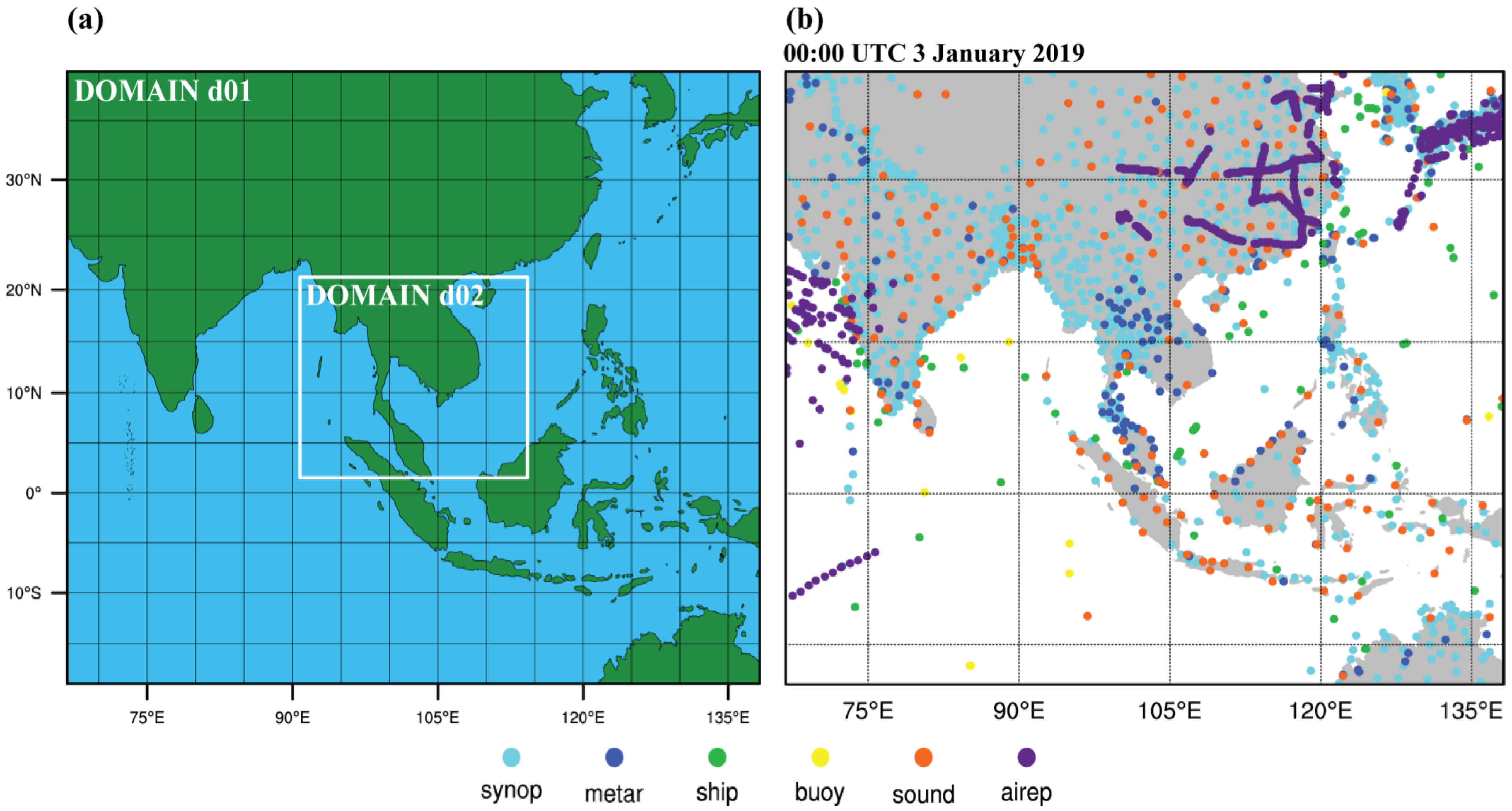
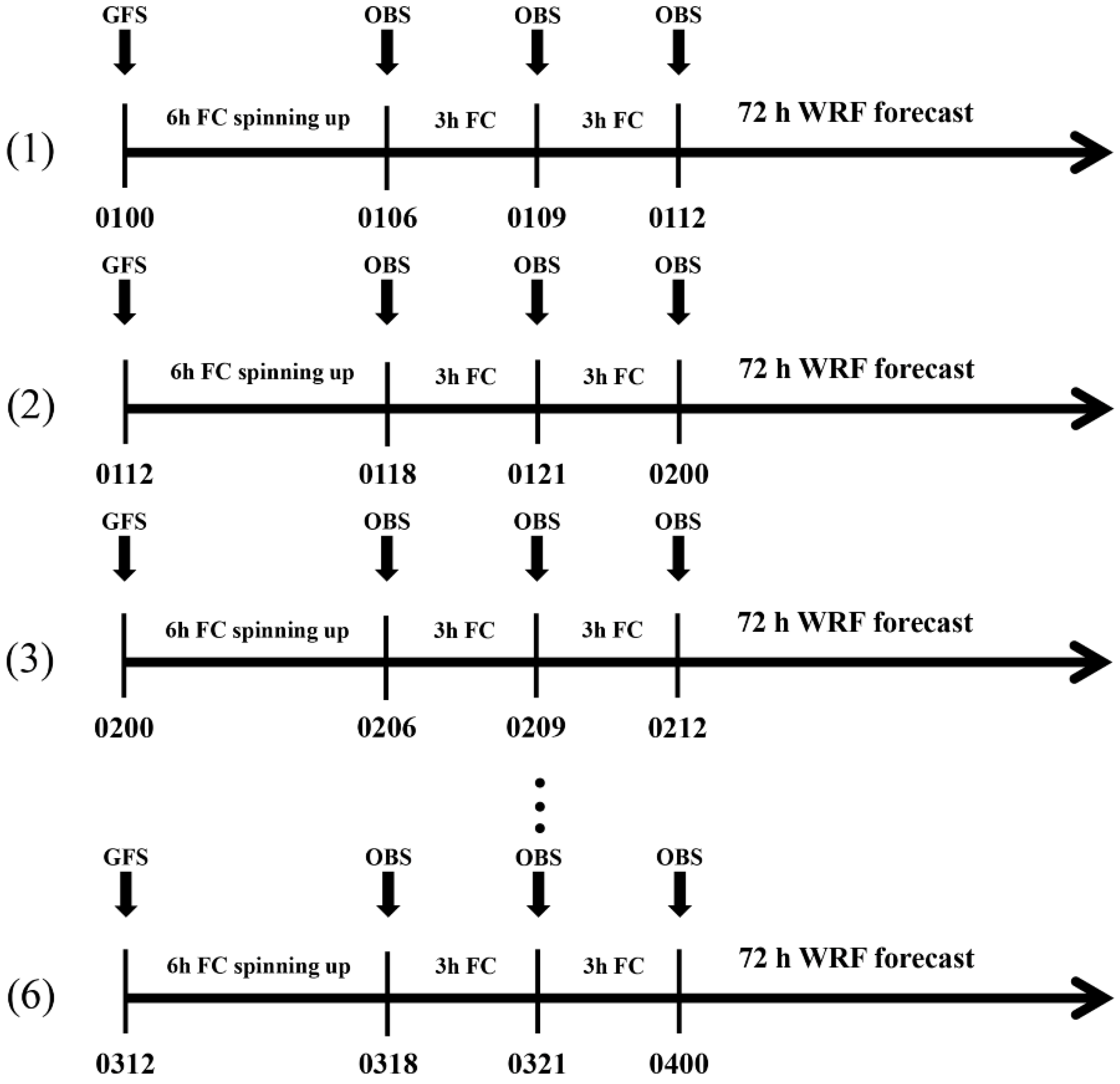
3.2. WRF Model Configurations and Experimental Setup

The Advanced Research WRF model version 3.9.1.1 [31] developed by the National Center for Atmospheric Research (NCAR) was utilised. It provides a state-of-the-art atmospheric simulation system. It improved the physics options and included multiple re-locatable nesting schemes for the operational forecast and atmospheric research. The model used Arakawa C-grid staggering for the horizontal grid, while the vertical grid was implemented with a completely compressible system of equations and terrain-hydrostatic pressure coordinating with vertical grid stretching. A third order Runge–Kutta scheme [32] was utilised for a time-split integration with a smaller time-step for acoustic and gravity wave modes. The WRF model physical parameterization option sets for hurricane application nesting used by NCAR’s real-time hurricane runs, consisted of the WRF Single Moment 6 class (WSM6) microphysics scheme [33], the Tiedtke cumulus convection parameterization scheme [34,35], and the Yonsei University planetary boundary layer scheme [36,37]. The RRTMG scheme [38] was utilised for both long-wave and short-wave radiation. A multilayer Noah land surface model was also employed in the soil modelling scheme [39]. This study chose air-sea flux parameterization schemes based on the Garratt formulation, which changes the enthalpy coefficients of the air-sea flux parameterization scheme [40]. All of the experiments employed WRFDA’s control variable option 5 (stream function, unbalanced velocity potential, unbalanced temperature, unbalanced surface pressure, and pseudo relative humidity) [41,42]. The background error covariance (BEC) was estimated using statistics of the differences between 12 h and 24 h forecasts for the period 1 November 2018 to 31 January 2019, based on the National Meteorological Centre (NMC) method [43,44]. Data thinning was often required and when using high-density AMVs, a 20 km thinning resolution was applied for all AMVs experiments (FY2G, FY4A, and HIM8) [45]. In all the experiments, two-way interactive nested domains were conducted for the prediction of TCs, with a horizontal resolution of 12 km with 650 * 640 grid points in the outer domain and 4 km with 560 * 550 grid points in the inner domain, respectively (Figure 3a). The model was set up with 36 vertical levels, with the model’s top level at 20 hPa. The cumulus parameterization was disabled in the inner domain for this study. To prepare the modelling analysis, data assimilation was performed in the outer domain for each experiment, and the impact of the AMVs data was analysed in the inner high-resolution domain.

For simulating TC PABUK using the WRF model, four sets of numerical experiments were conducted from six different initial conditions (every 12 h) with and without AMVs assimilation available from the FY-2G, FY-4A, and HIMA-8 satellites. The first experiment was a control experiment (hereinafter, “CONV”) used solely as conventional observations and was based on a dataset from the NCEP PREPBUFR (Prepared Binary Universal Form for the Representation of Meteorological Data) file. Radiosondes, ships, aircraft reports, synoptic observations, and airport reports were among the conventional observations utilised for the assimilation, with the exception of satellite-derived winds, whose distribution at 00:00 UTC 3 January 2019 was shown in Figure 3b as an example. The second experiment (hereinafter, “FY2G”) assimilated the same conventional observations as CONV with FY-2G AMVs from the IR and WV channels. The third experiment (hereinafter, “FY4A”) assimilated the same conventional observations as CONV with FY-4A AMVs from the IR, HIWV, and LOWV channels. The final experiment (hereinafter, “HIM8”) employed the same configuration but used CIMSS HIMA-8 AMVs derived from the IR, CTWV, and CAWV channels; however, SWIR and VIS channels from the HIMA-8 were not assimilated for a fair comparison.

Table 1. Description of the four sets of assimilation experiments at different initial conditions every 12 h. All AMVs observation selection for experiments at QI 85% start from 1 to 3 January 2019.

Experiments Name	Data used for Assimilation to d01	Forecast Initial Time	Forecast Hours
CONV	Conventional * (No AMVs)	06UTC 1 January	72
		18UTC 1 January	72
		06UTC 2 January	72
		18UTC 2 January	72
		06UTC 3 January	72
		18UTC 3 January	48
FY2G	Conventional * and FY-2G AMVs (IR, and WV)	06UTC 1 January	72
		18UTC 1 January	72
		06UTC 2 January	72
		18UTC 2 January	72
		06UTC 3 January	72
		18UTC 3 January	48
FY4A	Conventional * and FY-4A AMVs (IR, HIWV, and LOWV)	06UTC 1 January	72
		18UTC 1 January	72
		06UTC 2 January	72
		18UTC 2 January	72
		06UTC 3 January	72
		18UTC 3 January	48
HIM8	Conventional *and HIMA-8 AMVs (IR, CTWV, and CAWV)	06UTC 1 January	72
		18UTC 1 January	72
		06UTC 2 January	72
		18UTC 2 January	72
		06UTC 3 January	72
		18UTC 3 January	48

* Conventional refers to data that is taken from NCEP PREBUFR file.

shows the parameters and forecast initial times that were assimilated in the model.

Figure 4 depicts the flow charts of the partially cycling experiments conducted for this study. A total of six partially cycling analysis and forecast runs were performed at a frequency of 12 h for four experiments (CONV, FY2G, FY4A, and HIM8) from 06:00 UTC 1 January 2019 to 18:00 UTC 3 January 2019. With the NCEP GFS analysis as the background, each partially cycling run commenced with the first analysis 6 h earlier than the initial conditions times. Subsequently, three hourly analysis updates were obtained using a 3 h forecast initialized from the preceding cycle’s analysis as the background. Following the completion of three hourly cycle runs, 72 h forecasts were generated and gathered at 6 h intervals to assess the impact of the AMVs. The NCEP GFS analysis gave the lateral boundary conditions for 3 h and 72 h predictions.

4. Results

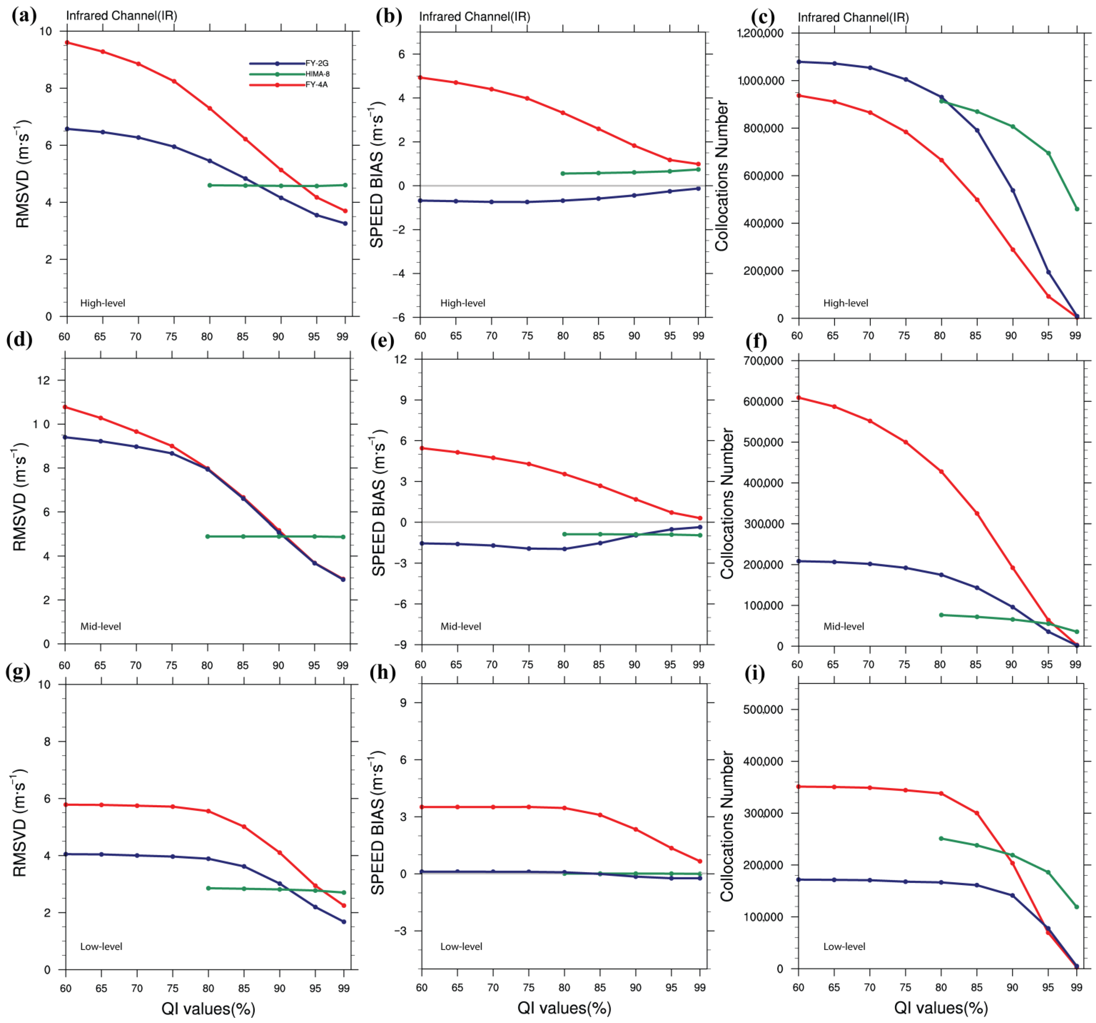
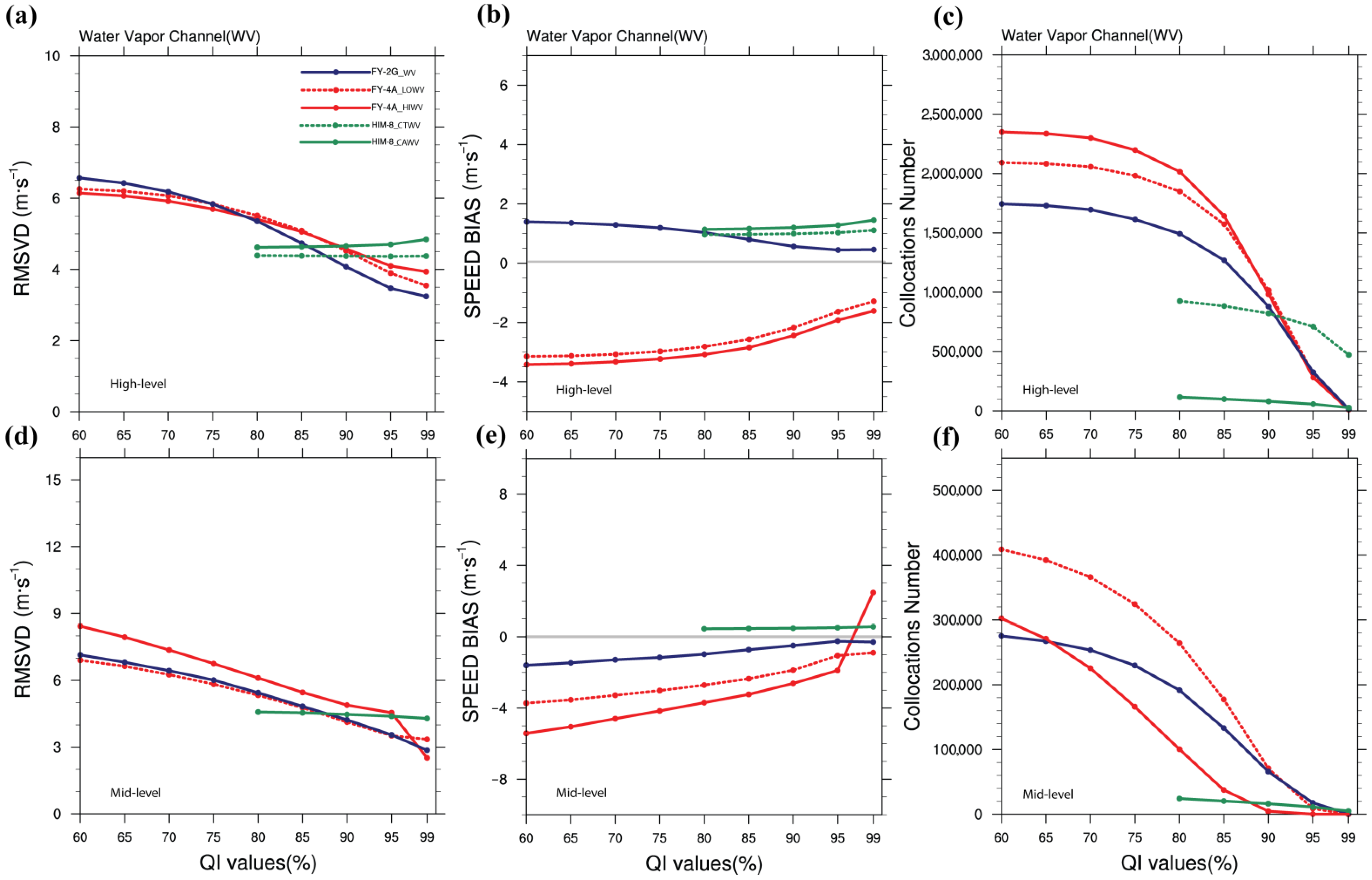
4.1. AMVs against NCEP FNL Wind Analysis Consistent with Diverse Quality Indicator Values

The quality indicator (QI) is a criterion for assessing the quality of AMVs. The percentage varies from 0 to 100% and the higher the QI value, the more credible it is [46]. It was important to demonstrate the sensitivity of accuracy according to different QI values in order to compare the AMVs from the three satellites of characterization and their impact, including introducing the new FY-4A AMVs to users. Users should be able to choose which AMVs are suitable to use for assimilation. For comparison study, all the AMV’s data was examined throughout three different, broad atmospheric levels at a low-level (>700 hPa), mid-level (400 to 700 hPa), and high-level (<400 hPa) for the same period.

In December 2018, the mean RMSVD, BIAS, and number of collocations of infrared AMVs for the different levels from all three satellites were collocated with corresponding NCEP FNL wind analysis, utilising varying QI values from 60 to 100% (Figure 5). The HIMA-8 AMVs were not available if the QI was less than 80%, unlike in the other cases. The results demonstrate that the RMSVD was not sensitive to variable QI values at all levels in the case of the HIMA-8. The RMSVD values for the high, mid, and low levels were around 4.6 m/s, 4.9 m/s, and 2.8 to 2.9 m/s, respectively, for any quality; however, the cases of the FY-2G and FY-4A were similar and the RMSVD was very sensitive to the varied QI values (Figure 5a,d,g), with its credibility being higher as one moved to higher QI thresholds, at the high, mid, and low-levels. The RMSVD value for any quality of the FY-2G (FY-4A) was as high as 6.6(9.6) m/s for the high-level, 9.4(10.8) m/s for mid-level, and 4.1(5.8) m/s for low-level. It dropped to 4.1(5.1) m/s for the high-level, 5.0(5.1) m/s for mid-level, and 3.0(4.1) m/s for low-level, respectively, if the QI was considered as being 90%. The FY-4A IR AMVs were extremely sensitive to QI values in the BIAS (Figure 5b,e,h). At all levels, the BIAS was positive and greater than the other two sets; the range was 0.3 to 5.1 m/s. The mid-level case of the FY-2G was mildly responsive (Figure 5e); the BIAS range was −1.6 to 0.1 m/s. For the HIMA-8 AMVs, the BIAS was not affected by changing QI values; the BIAS range was −0.9 to 1.0 m/s; however, when the total number of collocations was considered (Figure 5c,f,i), it was discovered that three sets of IR AMVs at high-levels were very sensitive to the QI values, and the number of collocations decreased dramatically as the QI values increased (Figure 5c). Only FY4 AMVs at the mid-level declined dramatically with increasing QI values (Figure 5f). The FY-2G and HIMA-8 declined dramatically at the mid- and low-levels, with QI values at 90% (Figure 5i).

For water vapour AMVs in December 2018, the RMSVD, BIAS, and number of collocations with varied QI values are shown in Figure 6. Comparable to infrared AMVs, the RMSVD (Figure 6a,d) and BIAS (Figure 6b,e) were sensitive to the QI values in the case of the FY-2G and FY-4A, while the number of collocations was also quite sensitive at all levels (Figure 6c,f). In the case of the HIMA-8, differing QI values had no impact on it. A positive BIAS was shown for the FY-2G and HIMA-8 at the high-level, whereas the FY-2G and FY-4A were negative at the mid-level. If QI values more than 85% were considered, it was found that the number of collocations reduced dramatically, leaving too few collocations, in comparison to the RSMVD and the BIAS, which had altered little.

As a result, with the QI at 85%, the RMSVD (IR and WV) values of all three satellites for any quality varied between 4.4 and 6.2 m/s for the high-levels, 4.5 to 6.7 m/s for the mid-levels, and 2.8 to 5.0 m/s for the low-levels. The BIAS (IR and WV) values of all three satellites for any quality ranged from −2.8 to 2.6 m/s for the high-levels, −3.2 to 2.7 m/s for the mid-levels, and −0.9 to 3.1 m/s for the low-levels. The RMSVD and BIAS values from the three satellites were comparable at the high, mid, and low levels with a few exceptions, while the number of collocations was not too small. Taking the volume and quality of the data (RMSVD, and BIAS) of the IR and WV from the three satellites into consideration, AMVs with a QI of 85% will be chosen from the products for further investigation.

4.2. Comparisons of FY-4A, FY-2G AMVs, and HIMA-8 AMVs Data at QI 85%

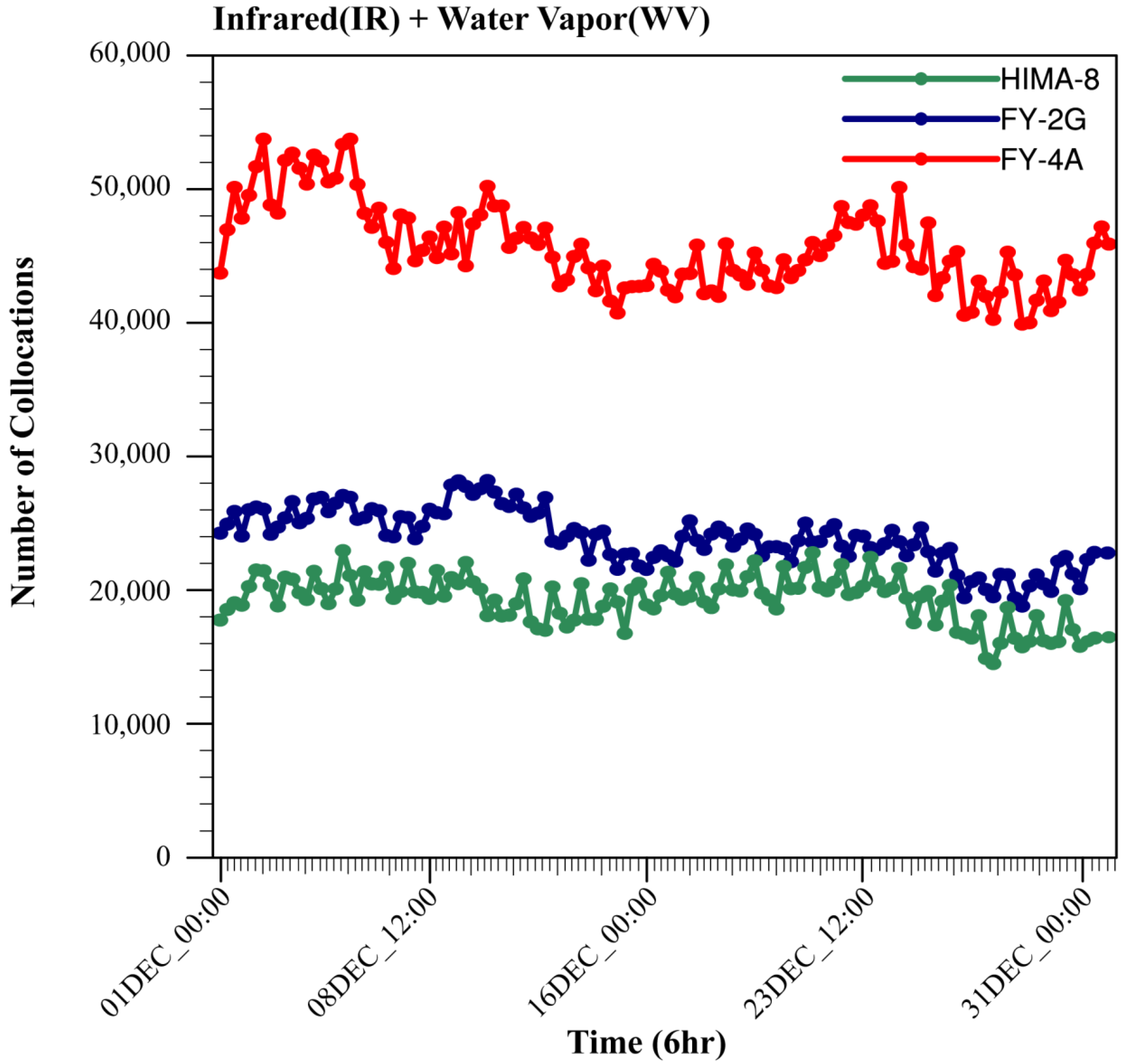
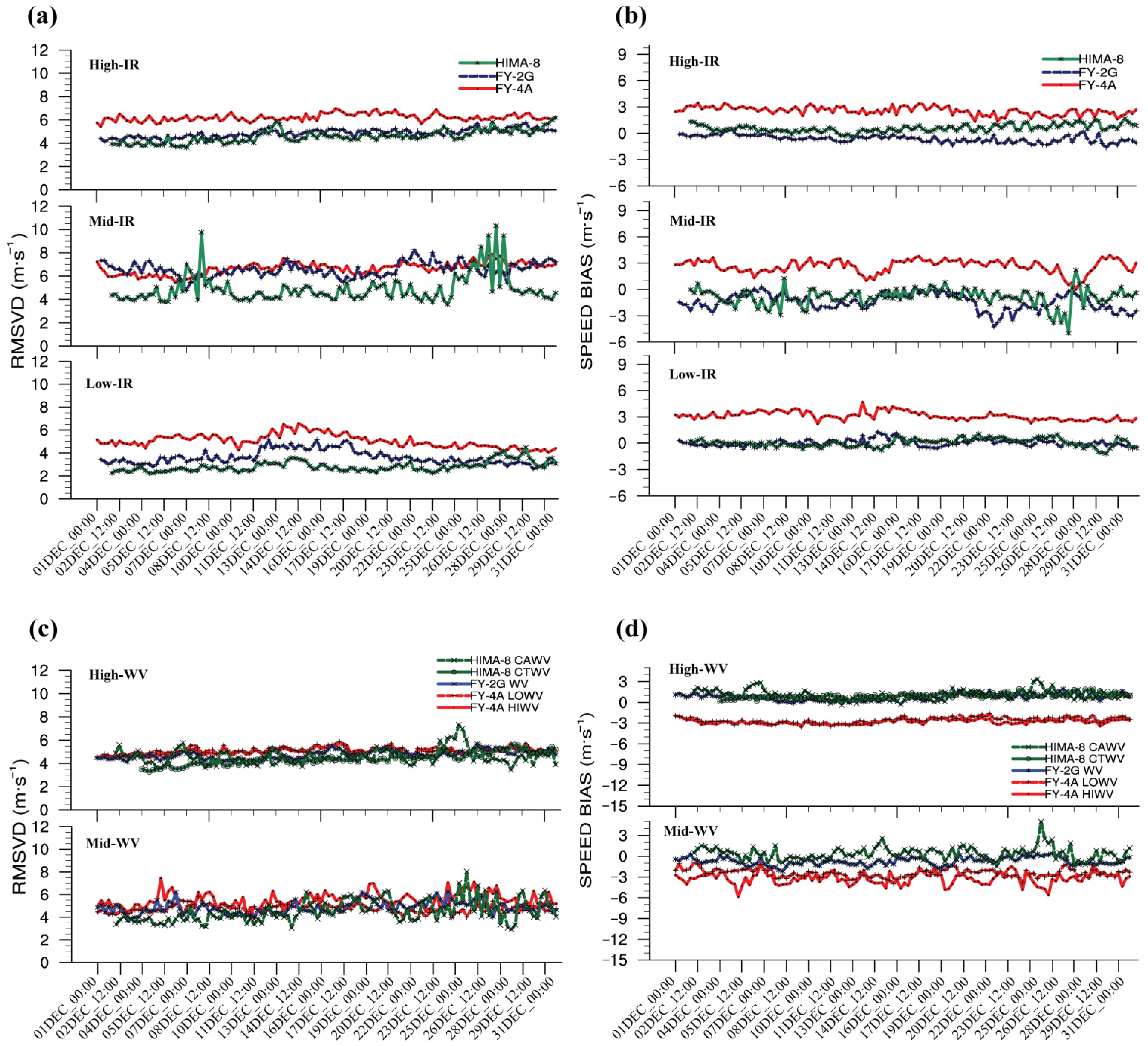
In this section, three sets of AMVs with QI 85% are examined in their time series, horizontal, and vertical structures before being applied to WRFDA-3DVar to analyse their variations in assimilation and forecasting.

4.2.1. Time Series

Figure 7 depicts the time series of the RMSVD and BIAS at QI 85% of the FY-2G, FY-4A, and HIMA-8 infrared and water vapour AMVs at high, mid, and low-levels, averaged over the research domain taken four times a day in December 2018. In the case of infrared AMVs, the RMSVD from the HIMA-8 AMVs was somewhat better at all levels than the other two sets (Figure 7a). For the FY-4A, the RMSVD was higher in high and low-levels than in the FY-2G and HIMA-8 for the individual 6 h time-period. The FY-2G and HIMA-8 had comparable BIAS properties (Figure 7b), whereas the FY-4A had positive values and a greater error. In the case of water vapour AMVs, the RMSVD of all three versions was similar in nature with a few exceptions (Figure 7c). The BIAS of FY-2G and HIMA-8 were comparable (e.g., positive speed bias), whereas the BIAS of the FY-4A showed a negative speed bias at high and mid-levels (Figure 7d).

Table 2. Monthly comparison of homogeneous samples of FY-2G, FY-4A and HIMA-8 infrared AMVs with respect to NCEP FNL wind analysis for different atmospheric levels over the retrieval domain at QI 85% for the three months starting from 1 November 2018 to 31 January 2019.

	FY-2G			FY-4A			HIMA-8
	High	Mid	Low	High	Mid	Low	High	Mid	Low
Nov-18
RMSVD	4.8	6.51	3.35	6.36	6.48	4.87	4.41	4.15	2.42
BIAS	−0.59	−0.92	−0.12	2.9	3.16	3.21	0.66	−0.42	0.14
NC *	747,216	145,120	202,812	436,959	291,448	366,732	820,055	61,627	245,949
Dec-18
RMSVD	4.83	6.61	3.62	6.21	6.66	5.02	4.59	4.89	2.84
BIAS	−0.59	−1.52	−0.01	2.59	2.68	3.1	0.58	−0.87	0.01
NC *	790,555	143,295	16,1222	498,574	324,989	300,173	869,395	71,921	237,993
Jan-19
RMSVD	4.9	6.81	3.36	6.3	6.9	4.92	4.72	4.77	2.72
BIAS	−0.48	−1.43	−0.03	2.43	2.32	3.17	0.84	−0.74	−0.12
NC *	637,215	160,692	225,263	383,339	294,292	424,238	753,067	60,960	318,849

* NC refers to numbers of collocations of AMV data.

shows the monthly mean RMSVD, BIAS, and number of collocations of homogenous samples of three sets of IR AMVs with regard to NCEP FNL wind analysis over the research domain from 1 November 2018 to 31 January 2019 at a QI of 85%. In terms of the RMSVD, it can be noted that the RMSVD of the IR AMVs at the high and mid-levels for all three sets was comparable. For all months, the HIMA-8 IR AMVs exhibited a somewhat superior RMSVD in the low-level compared to the other two sets. For the WV AMVs (

Table 3. Monthly comparison of homogeneous samples of FY-2G, FY-4A, and HIMA-8 water vapour AMVs with respect to NCEP FNL wind analysis for different atmospheric levels over the retrieval domain at QI 85% for the three months starting from 1 November 2018 to 31 January 2019.

	FY-2G		FY-4A				HIMA-8
	WV		HIWV		LOWV		CTWV		CAWV
	High	Mid	High	Mid	High	Mid	High	Mid	High	Mid
Nov-18
RMSVD	4.69	4.95	5.18	5.46	5.06	4.91	4.17	-	4.42	4.4
BIAS	0.64	−0.98	−3.05	−3.03	−2.61	−2.32	0.94	-	0.75	0.39
NC *	1,251,666	153,818	1,577,073	51,333	1,415,997	230,033	882,554	-	98,795	20,331
Dec-18
RMSVD	4.74	4.83	5.06	5.46	5.09	4.77	4.38	-	4.63	4.55
BIAS	0.8	−0.72	−2.84	−3.24	−2.57	−2.36	0.97	-	1.16	0.46
NC *	1,268,636	133,206	1,642,542	37,445	1,572,873	177,435	93,9433	-	73,758	12,105
Jan-19
RMSVD	4.87	5.09	4.87	6.28	5.07	5.39	4.53	-	4.89	4.91
BIAS	0.98	−0.66	−2.35	−3.65	−2.29	−2.7	1.13	-	1.34	0.19
NC *	1,041,683	140,649	1,512,157	33,524	1,294,358	119,479	836,825	-	70,867	11,459

* NC refers to numbers of collocations of AMV data.

), the RMSVD for all three sets was likewise comparable, with a few exceptions. In terms of the BIAS, the FY-2G and HIMA-8 had identical BIAS characteristics for both the IR and WV AMVs. For all levels, the HIMA-8 and FY-2G (IR and WV) AMVs were more accurate than the FY-4A. In terms of collocations, the FY-4A had a substantially greater number of collocations than the FY-2G and HIMA-8 at the low and mid-levels.

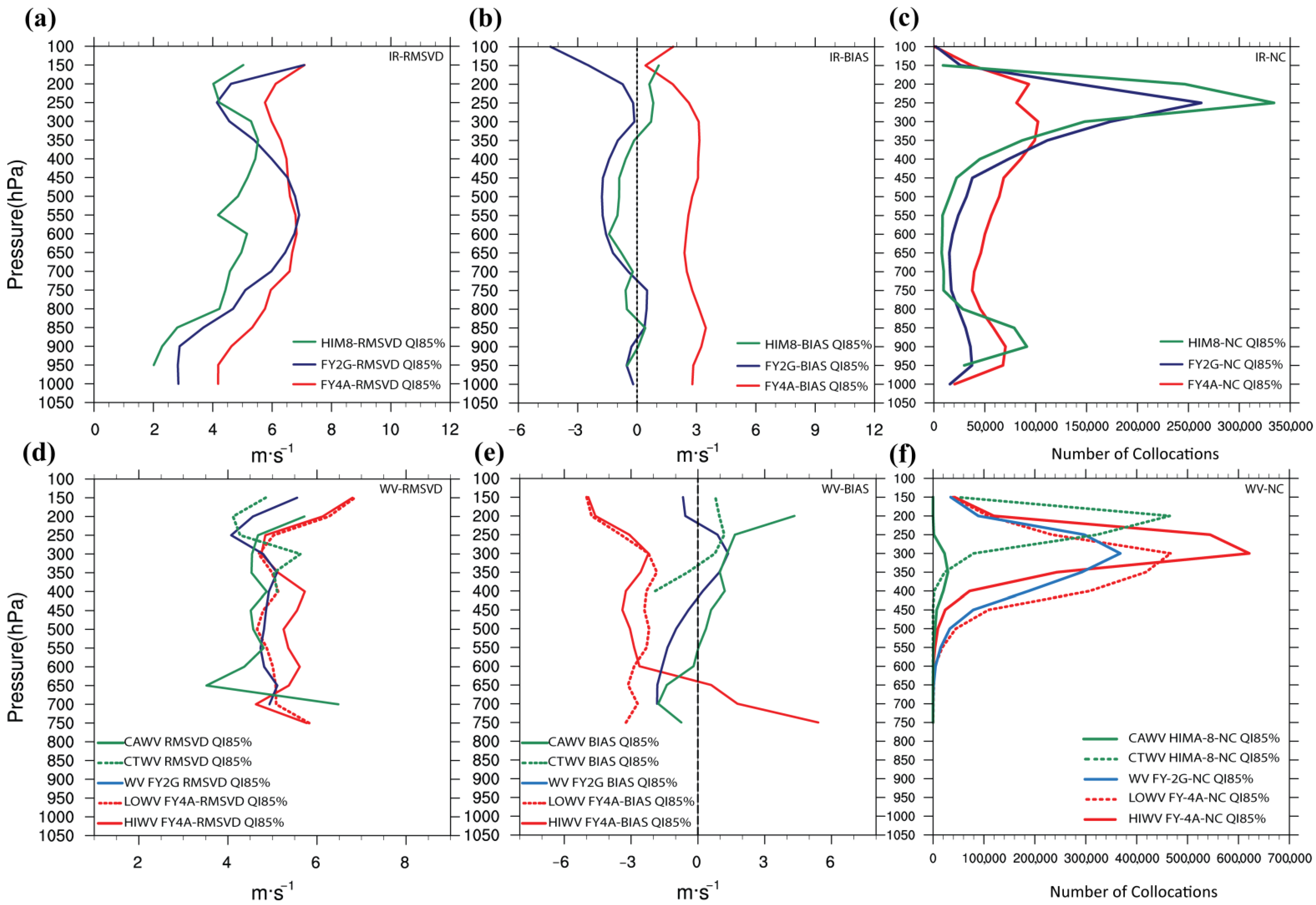
4.2.2. Vertical Profile

Figure 8 illustrates the vertical profiles of the RMSVD, BIAS, and total number of collocations in December 2018 for both the IR and WV AMVs. The vertical distribution of the RMSVD IR and WV AMVs obtained from the three satellites are depicted in Figure 8a,d, respectively. The RMSVD for all three sets of IR AMVs was similar in nature, as shown in Figure 8a. The RMSVD increased with the height from low to mid-levels, then decreased to the high-level until 250 hPa. In the mid-level between 400 and 700 hPa, however, the HIMA-8 IR AMVs outperformed the two other sets. The RMSVD WV AMVs in Figure 8d were comparable for all satellites, except for the mid-level, where the HIMA CAWV from the HIMA-8 was somewhat better than the other sets.

The vertical distribution of the BIAS IR and WV AMVs, which were produced from three satellites, is depicted in Figure 8b,e, respectively. The BIAS of the FY-2G and HIMA-8 from the IR (Figure 8b) and WV (Figure 8e) AMVs exhibited a similar pattern. In the case of the FY4A AMVs, the BIAS IR AMVs were positive at all levels, the LOWV AMVs were negative at all levels, and the HIWV AMVs were positive at the mid-level, decreasing to negative as the height pressure levels rose (Figure 8e).

In general, the retrieval of the three sets of IR AMVs mostly dominated at high-levels at 150 to 400 hPa, as seen in Figure 8c. At all levels, the HIMA-8 and FY-2G IR AMVs had similar numbers of collocations. Although there were fewer collocations at the high-level among the FY-4AIR AMVs than in the other two sets, there were more rising numbers in the mid-level between 400 to 700 hPa. For WV AMVs, the FY-4A HIWV AMVs had a higher number of collocations at the high-level than the other sets. Because there were no WV AMVs below 700 hPa, the number of collocations of the three sets of WV AMVs was mostly dominated at the high-level (Figure 8f).

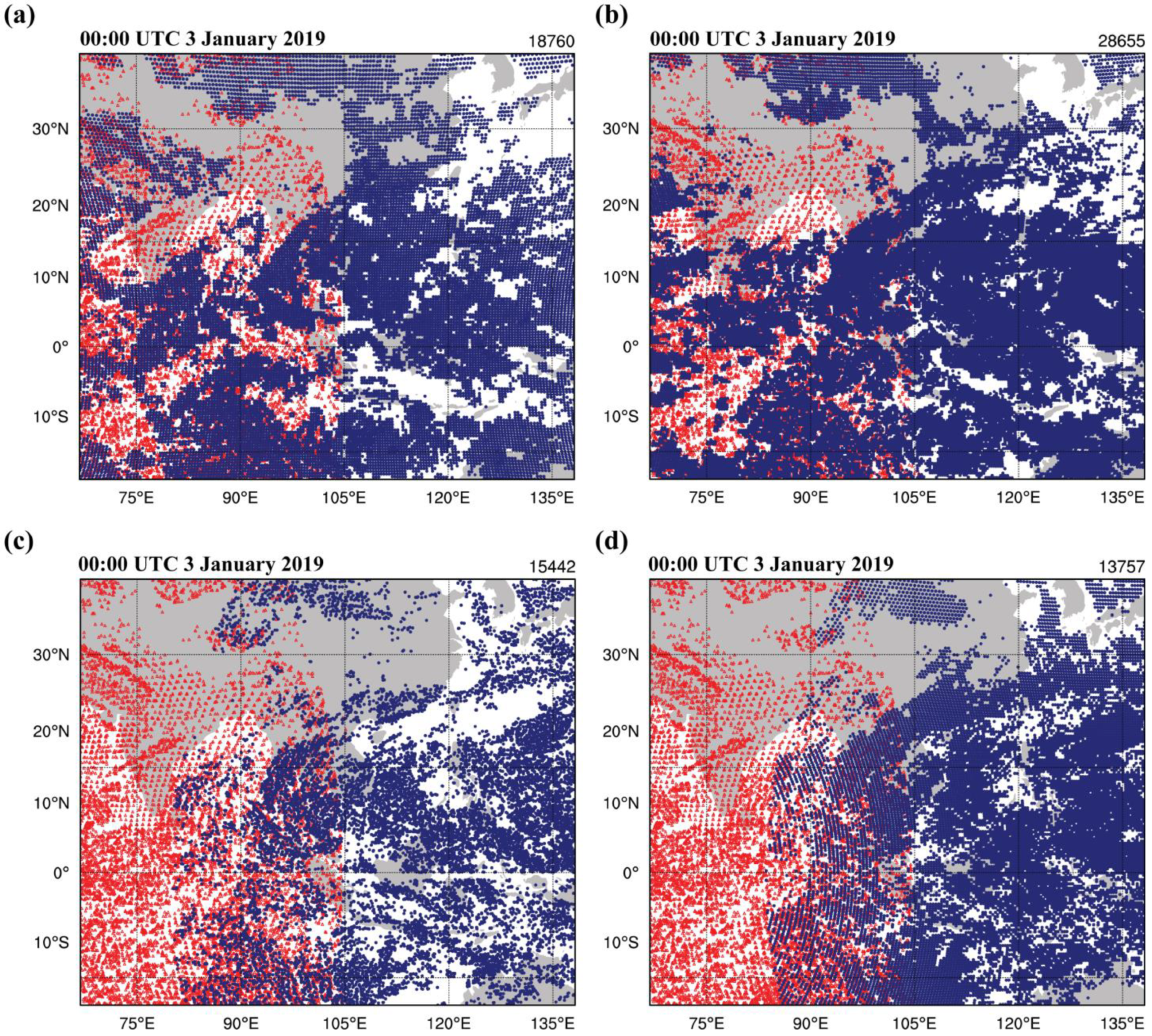
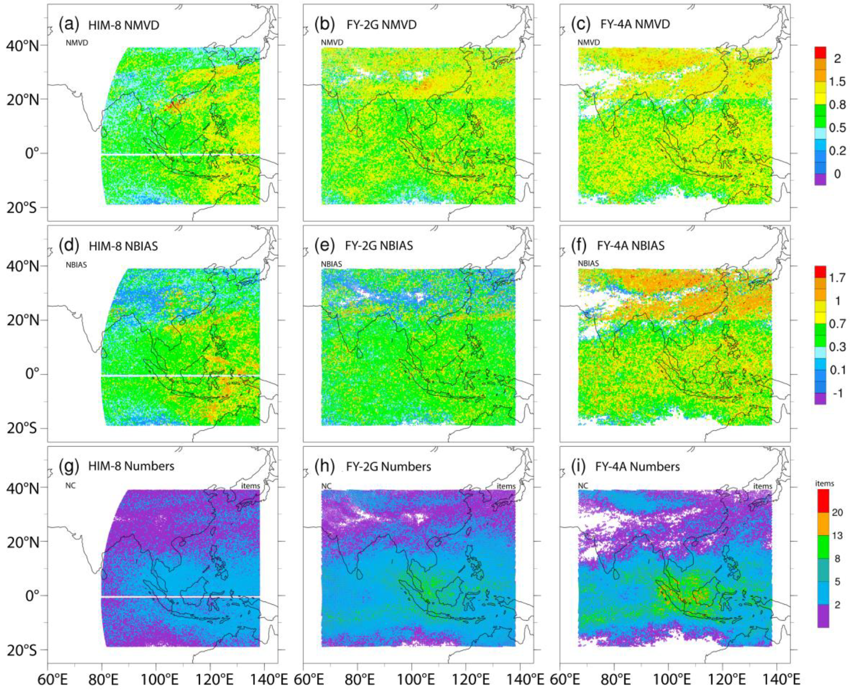
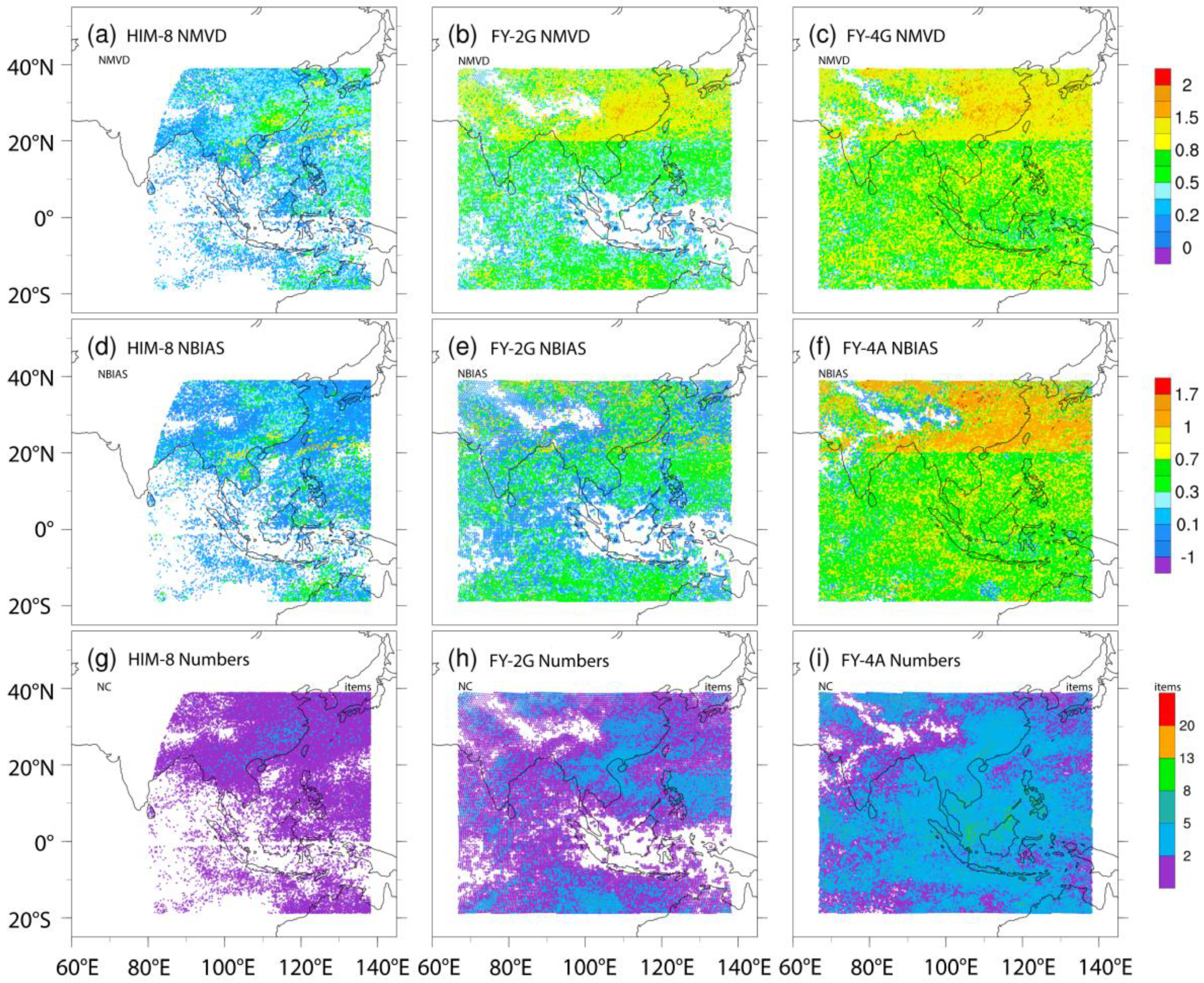
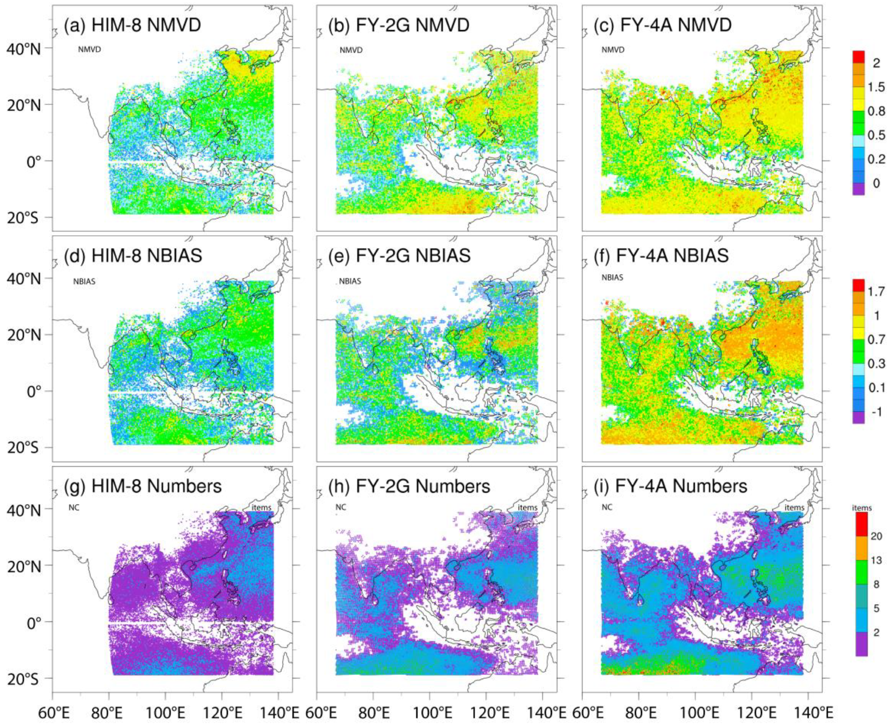
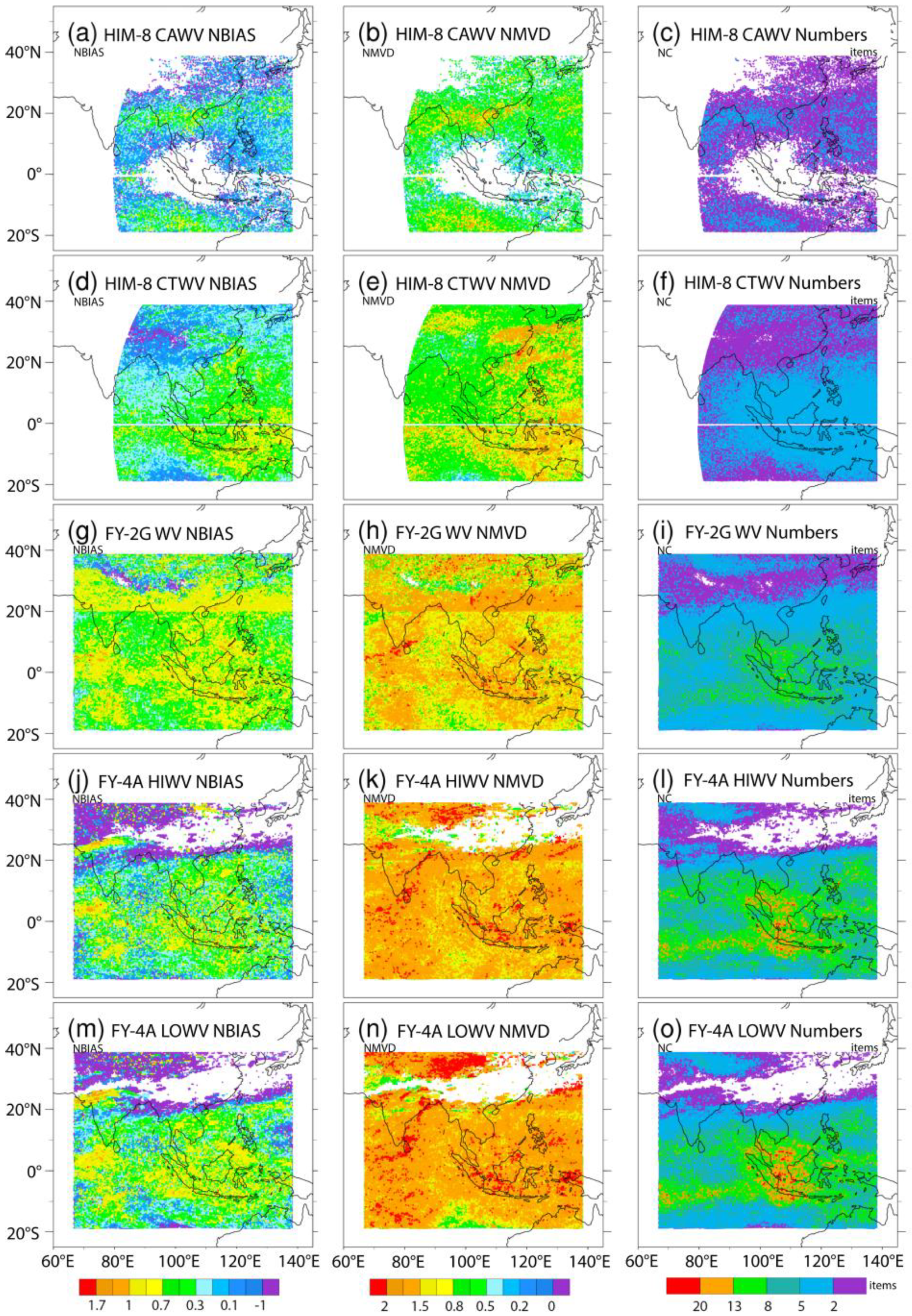
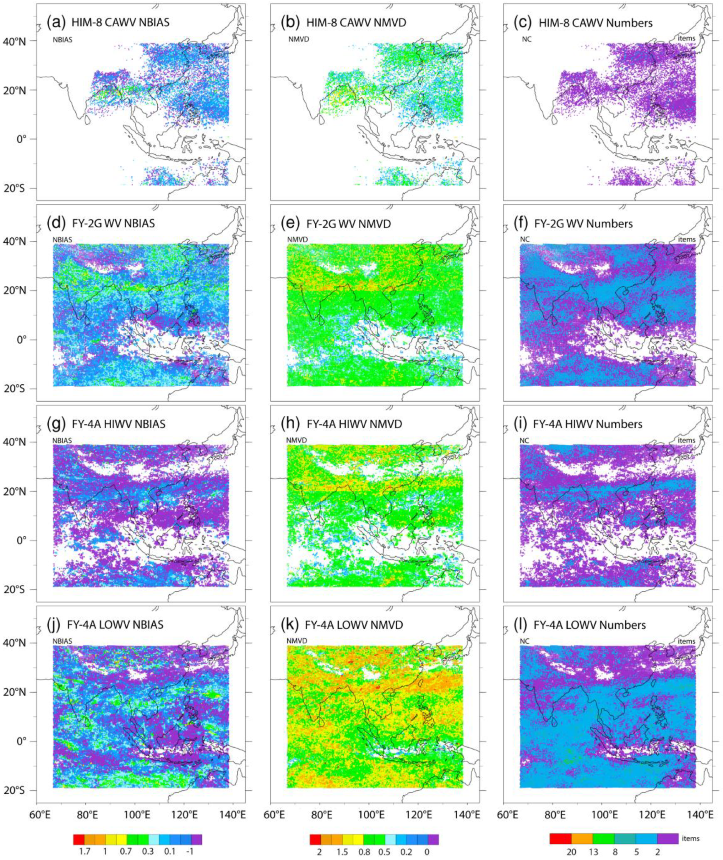
4.2.3. Horizontal Distributions

When IR and WV AMVs from the FY-2G, FY-4A, and HIMA-8 AMVs were collocated with NCEP FNL wind analysis in December 2018, the spatial pattern plots of NMVD and NBIAS were compared on average, including that of the number of collocations. For the IR AMVs, the NMVD for all three sets of IR AMVs was consistent at the high-level (Figure 9a–c); however, compared to the other two sets, the FY-4A AMVs had fewer collocations at higher latitudes (Figure 9i), were predominantly located in the tropics, and had slightly larger NMVD values, notably in the extra-tropics. When compared to the FY-4A AMVs, the HIMA-8 and FY-2G AMVs exhibited a greater and more uniform distribution of collocation numbers (Figure 9g,h). The NBIAS pattern for the FY-2G and HIMA-8 of the IR AMVs (Figure 9d–f) were comparable with few exceptions. In the tropics, the NBIAS from the FY-2G and HIMA-8 were positive, while in the extra-tropics, they were negative (Figure 9d,e); however, the NBIAS for the FY4A had more positive values than the other two sets in both the tropics and extra-tropics (Figure 9f).

For the mid-level, the NMVD (Figure 10a–c) and NBIAS (Figure 10d–f) for all three sets of AMVs were also similar, as shown at the high-level. Nonetheless, relative to the HIMA-8 and FY-2G, the FY-4A had a greater number of collocations (Figure 10i), with the NMVD (Figure 10c) and NBIAS (Figure 10f) significantly higher in both the tropic and extra-tropic regions. Similarly, it was demonstrated in the mid-level, as for the low-level (Figure 11). The pattern of the NMVD (Figure 11a–c) and NBIAS (Figure 11d–f) of AMVs from three satellites at low-level has similar characteristics. The total collocation in FY-4A is much higher compared to FY-2G and HIMA-8 (Figure 11g–i). However, the HIMA-8 AMVs still have better NMVD, slightly smaller NBIAS compared to other two sets especially in the extra-tropics region.

In the case of WV AMVs at the high-level, the NBIAS of the CTWV, FY-2G WV, HIWV, and LOWV were comparable, becoming positive throughout the retrieval domain in the tropical region (Figure 12d,g,j,m), but negative in the extra-tropics. For the CAWV of the HIMA-8 AMVs (Figure 12a), the NBIAS differed somewhat in the tropical region due to decreased collocations in this domain from the others (Figure 12c). The NMVD for the WV from the FY-2G (Figure 12h) and two WVs (HIWV and LOWV) from the FY4A (Figure 12k,n) were comparable and greater than the NMVD for the CAWV and CTWV from the HIMA-8 (Figure 12b,e) across the research domain. When compared to the HIMA-8 and FY-2G WV AMVs, the HIWV and LOWV had a greater number of collocations (Figure 12l,o), with the majority of the data collocated across the tropic region (Figure 12c,f,i). For the mid-level, the NBIAS (Figure 13a,d,g,j) and NMVD (Figure 13b,e,h,k) for all three sets of WVAMVs were also similar, with the quantities of collocations of the FY-2G and FY-4A being comparably greater than the HIMA-8 (Figure 13c,f,i,l); however, the case of the LOWV from the FY-4A had more errors than the other two sets. It can be seen that the mid- and high levels of the atmospheric wind data received potential benefits from an increased data amount from the FY-2G and FY-4A over the study domain.

4.3. Impaction Data Assimilation

The impact of AMVs on the assimilations for assessment of the initial position and forecasting of the track and intensity from the inner domain of TC PABUK is presented in this section by calculating the average values of the TC track, minimum MSLP, and maximum surface wind difference from Joint Typhoon Warning Centre (JTWC) data.

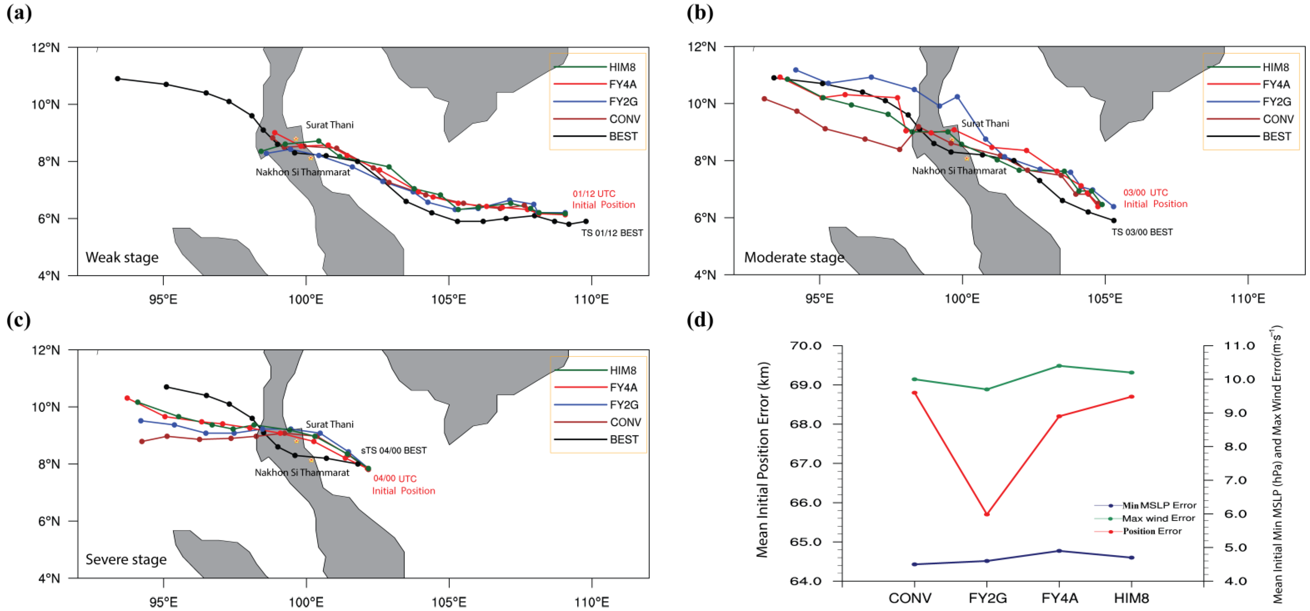
4.3.1. Initial Position Error

The simulated initial positions were determined utilising the centre of minimum MSLP contours compared to a JTWC best-track analysis to assess the initial position error. Figure 14a–c illustrates some examples of WRF simulations from four experiments, CONV (brown), FY2G (blue), FY4A (red), and HIM8 (green), in terms of the initial positions and forecasted tracks taking into consideration the TC PABUK stages, namely, weak (Figure 14a), moderate (Figure 14b), and severe (Figure 14c). The black line is the JTWC (hereinafter, “BEST”) best-track for TC PABUK.

The initial position from all experiments at the weak and moderate stages was not significantly different, with a higher inaccuracy than the severe TC stage compared to the BEST. This implies that in this TC example, the AMVs were more successful at minimising initial position errors at the severe TC stage than at the weak TC stage. Figure 14d compares the average initial position errors of the four experiments (red). Here, the averages were calculated based on six different initial conditions in each experiment. When compared to the CONV experiment, the average initial position errors improved marginally after assimilating the AMVs in the FY2G, FY4A, and HIM8. The FY2G had a greater positive impact on the average initial position than the FY4A and HIM8. The average initial position error in the CONV was 68.8 km, whereas it was 65.7, 68.2, and 68.7 km in the FY2G, FY4A, and HIM8, respectively. This demonstrates that the assimilating AMVs of three experiments had a somewhat beneficial influence on the TC initial position errors.

4.3.2. Initial Intensity Error

The impact of AMVs on assimilation for intensity errors was determined by comparing the maximum surface winds and minimum MSLP amplitude to JTWC best-track analyses. As seen in Figure 14d, the average initial maximum surface wind (green) for the CONV experiment was 10.0 m/s, but for the FY2G, FY4A, and HIM8, it was 9.8, 10.4, and 10.2 m/s, respectively. The average initial minimum MSLP (blue) for the CONV was 4.5 hPa, whereas it was 4.6, 4.9, and 4.7 hPa for the FY2G, FY4A, and HIM8, respectively. It was discovered that the assimilation of the FY4A and HIM8 AMVs seemed to have no impact on the initial intensities when measured in the initial maximum surface wind and minimum MSLP.

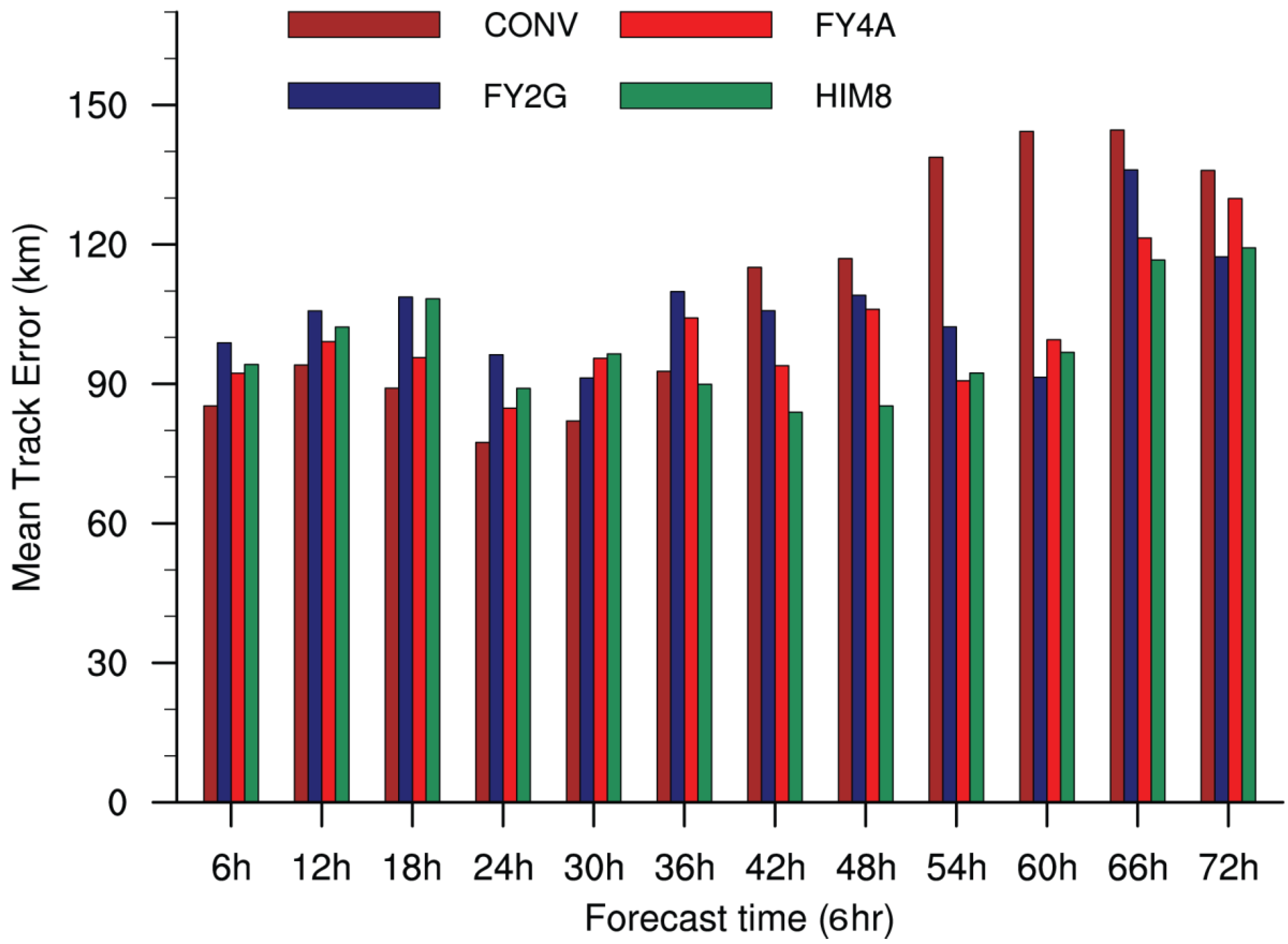
4.3.3. Track Forecasts

For each experiment, 72 h simulations were performed. The track and intensity forecasts were gathered at 6 h intervals and compared to JTWC best-track analyses for verification. As seen in Figure 14a, the simulated TC track from all experiments was similar, which correlates well with the JTWC observed best-track, while the TC was at the weak stage. In Figure 14b, the track forecasts for the FY4 and HIM8 up to 30 h were improved in comparison to the FY2G and 48 h relative to the CONV. During the severe period of the TC, the landfall prediction track was also observed as shown in Figure 14c. This demonstrates that none of the experiments could capture the landfall accurately. The model forecasted a landfall position closer to the Surat Thani coast rather than the actual landfall position located adjacent to the Nakhon Si Thammarat coast. Nevertheless, it was revealed that the FY4A had a greater impact than the other experiments up to 24 h in this stage. It was observed that the moderate and severe TC stages had a greater influence on the tracking inaccuracy than in the weak stages of assimilating the AMVs; however, while the TC was landing toward the coast, the forecast was still erroneous owing to other factors such as the terrain influence.

Figure 15 depicts the average track errors for each 6 h forecast from all four sets of experiments. It is noted that in all the AMVs experiments (e.g., FY2G, FY4A, and HIM8), the impact of AMVs was mostly positive between the 42 h and 72 h forecast lead times as compared to the CONV. The 42 h prediction track errors in the FY2G, FY4A, and HIM8 were 105.7, 93.9, and 83.9 km, respectively, whereas the error in the CONV was 115.1 km. The relative track forecast errors computed with respect to the CONV for the FY2G, FY4A, and HIM8 experiments were −8.1%, −18.4%, and −27.1%, respectively. The highest relative reduction occurred for the 60 h (36.6%) forecast for the FY2G, the 54 h (33.4%) forecast for the FY4A, and the 54 h (33.4%) forecast for the HIM8 experiment, respectively.

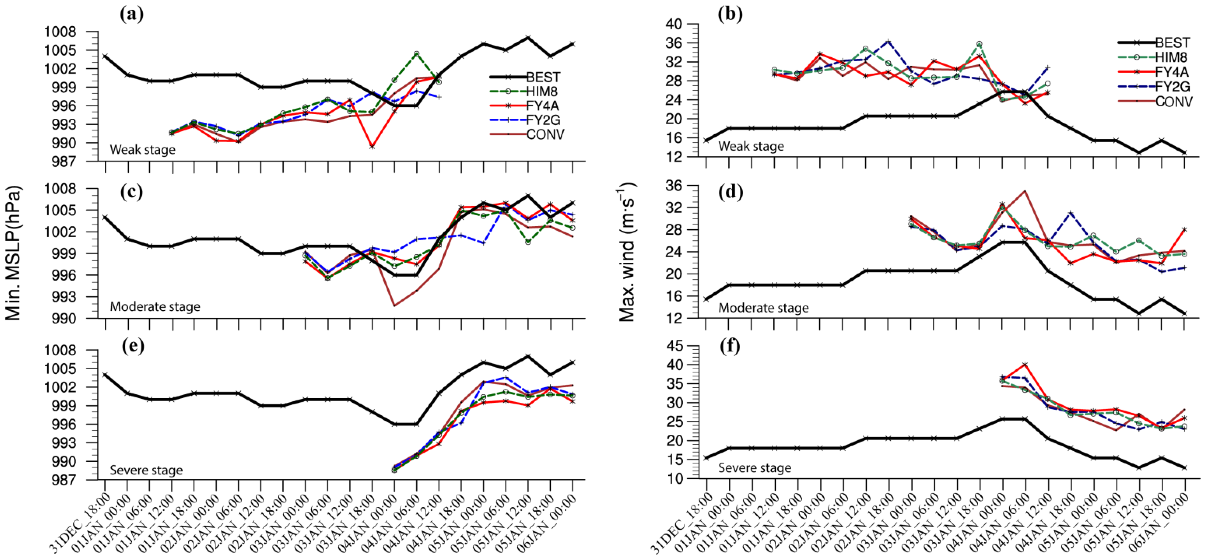
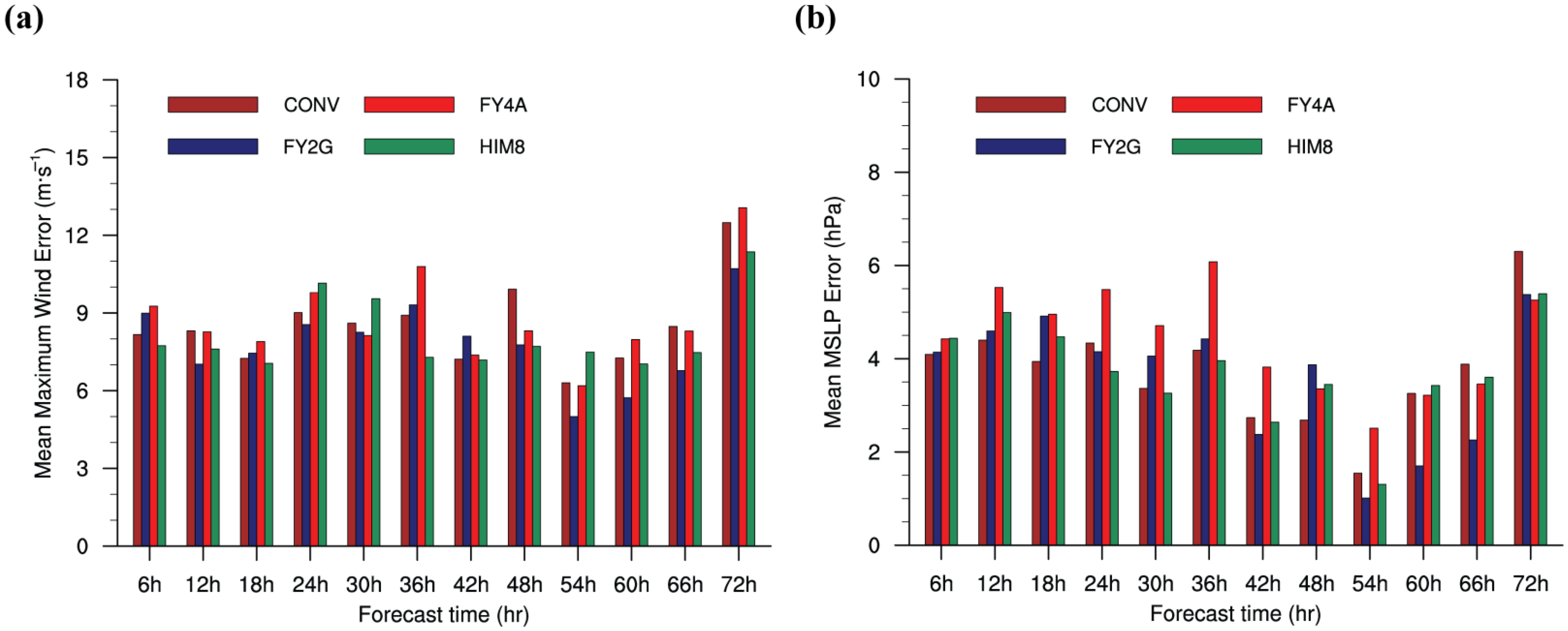
4.3.4. Intensity Forecasts

The temporal distribution of the minimum MSLP and maximum surface winds from the CONV, FY2G, FY4A, and HIM8 experiments for TC PABUK is given in Figure 16. The prediction of TC intensity began at 12:00 UTC 1 January 2019 (Figure 16a) at its weak stage. The predicted MSLP was over-estimated in all experiments. The simulated maximum surface wind speed from each experiment was similar and relatively strong compared to the BEST (Figure 16b). During its moderate stage, which began at 00:00 UTC on 3 January 2019 (Figure 16c), the predicted minimum MSLP matched the BEST well during the whole integrated period. The FY4A and HIM8 tended to correct the minimum MSLP when the integrated time was up to 24 h to 36 h compared to the CONV and FY2G; however, the maximum surface wind speed from all experiments also provided much stronger values, at a peak duration varying between 25.8 to 35.1 m/s, comparable to the peaked BEST (Figure 16d). At its severe stage, which began at 00:00 UTC on 4 January 2019, the minimum MSLP and maximum surface wind were over-estimated in all experiments (Figure 16e,f).

Figure 17 indicates the average maximum wind forecast errors and the average forecast of the minimum MSLP error from all four experiments for each 6 h forecast. It was discovered that the average maximum wind forecast error improvement from the AMVs experiments were not statistically significant compared to the CONV (Figure 17a). Similar results were seen for all experiments in the average MSLP as shown in Figure 17b, with the FY4A mostly more over-estimated in error terms than in the other experiments.

5. Conclusions

The present study proceeds to assess the preliminary qualityof AMVs retrieved from multi-channels of the FY-2G, FY-4A, and HIMA-8, as well as their impact on the track and intensity forecast of TC PABUK over SEA using the WRF model and 3D-Var data assimilation system. To obtain the reliability on the operation of the FY-2G AMVs and new FY-4A AMVs, an exactly similar comparison was repeated with previously available HIMA-8 AMVs over this region. The above results from the experiments indicate that:

• Regarding the AMV characteristics, three sets of derived AMVs were used for three months and were compared to NCEP/FNL operational global analysis data. The RMSVD, BIAS, and the number of collocations are highly sensitive to QI values for the FY-2G and FY-4A AMVs over the study domain, whereas the HIMA-8 AMVs are insignificant. As a result, the QI must be considered for usage for the FY AMVs series.
• As the considered QI was at 85%, the retrieval of the IR AMVs from the three satellites was mostly dominant at the high and low levels, whereas the WV AMVs were mostly dominant at high levels between 150 and 400 hPa. The qualities of the FY-2G and FY-4A AMVs were similar, and AMVs from the HIMA-8 generated more accurate totals than those from the FY-2G and FY-4A. Moreover, the monthly mean RMSVD and BIAS AMVs at all levels for the three satellites were comparable with few exceptions for all months; however, among them, the HIMA-8 AMVs have better accuracies compared to FY-2G and FY-4A AMVs.
• The qualities of the FY-2G and FY-4A were similar in nature throughout December 2018, and all WV AMVs were more consistent than IR AMVs. The FY-4A AMVs had a lower quality in the IR channel than the FY-2G AMV, but a comparable quality in the water vapor channel. Although the FY-4A AMVs had improved the spatial and temporal resolution data, the AMV products derived from the FY-4A satellite are still under research. Stricter processes should be conducted in the future for FY-4A AMVs’ quality control, which is necessary to reduce the spatial correlations and errors when employing high-density AMVs. After the second half of 2020, the algorithm for the FY-4A was improved [47]. The quality of the AMVs from the FY4A gradually stabilized after the algorithm improvement. Furthermore, the greater QI value of the FY-4A for using with assimilation should be further considered.
• Four experiments were conducted with and without the assimilation of AMVs from the FY-2G, FY-4A, and HIMA-8 at a QI of 85% via WRF 3D-Var to validate the impact of the AMVs. It was found that the assimilation from three satellites reduced the average initial position error slightly. After a 42 h integration time, the average forecast track error of the FY2G, FY4A, and HIM8 experiments was revealed to be lower than the control experiment (CONV). The HIM8 experiments mostly had more improved typhoon track forecasts than the FY4A and FY2A experiments, respectively. It was demonstrated that the availability of more IR and WV collocation numbers in the FY-2G and FY4A AMVs enhanced the impact of the AMVs on TCs, which have more opportunities with accessible satellites the same as the HIMA-8 over this region. Moreover, it was observed that the AMVs were more effective at the severe stage in reducing the initial positions and track errors rather than at the weak stage for TC PABUK; however, when compared to the control experiment, the initial and forecasted intensities for the TC were statistically insignificant in terms of improvement.

Despite the fact that this study was restricted to one cyclone and a small number of experiments, the preliminary examination provided information about the quality of the FY-2G, FY-4A AMVs, and HIMA-8, along with their potential impact on a cyclone track forecast for assimilating into operational NWP models. Supplemental case studies will be required in addition to the existing study in order to use the satellite products and evaluate their effectiveness over SEA.

References

1. Nieman, S.J.; Schmetz, J.; Menzel, W.P. A comparison of several techniques to assign heights to cloud tracers. J. Appl. Meteorol. 1993, 32, 1559–1568. [Google Scholar] [CrossRef]
2. Velden, C.S.; Hayden, C.M.; Nieman, S.J.; Menzel, W.P.; Wanzong, S.; Goerss, J.S. Upper-tropospheric winds derived from geostationary satellite water vapor observations. Bull. Am. Meteorol. Soc. 1997, 78, 173–195. [Google Scholar] [CrossRef]
3. Bedka, K.M.; Mecikalski, J.R. Application of satellite-derived atmospheric motion vectors for estimating meso-scale flows. J. Appl. Meteorol. 2005, 44, 1761–1772. [Google Scholar] [CrossRef]
4. Le Marshall, J.F.; Jung, J.; Zapotocny, T.; Redder, C.; Dunn, M.; Daniels, J.; Riishojgaard, L.P. Impact of MODIS atmospheric motion vectors on a global NWP system. Aust. Meteorol. Mag. 2008, 57, 45–51. [Google Scholar]
5. Leslie, L.M.; LeMarshall, J.F.; Morison, R.P.; Spinoso, C.; Purser, R.J.; Pescod, N.; Seecamp, R. Improved hurricane track forecasting from the continuous assimilation of high-quality satellite wind data. Mon. Weather Rev. 1998, 126, 1248–1257. [Google Scholar] [CrossRef]
6. Soden, J.B.; Velden, C.S.; Tuleya, R.E. The impact of satellite winds on experimental GFDL hurricane model forecasts. Mon. Weather Rev. 2001, 129, 835–852. [Google Scholar] [CrossRef]
7. Le Marshall, J.F.; Leslie, L.M.; Abbey, R.F.; Qi, L. Tropical cyclone track and intensity prediction: The generation and assimilation of high-density, satellite-derived data. Meteorol. Atmos. Phys. 2002, 80, 43–57. [Google Scholar] [CrossRef]
8. Wang, D.; Liang, X.; Duan, Y. Impact of four-dimensional variational data assimilation of atmospheric motion vectors on tropical cyclone track forecasts. Wea. Forecast. 2006, 21, 663–669. [Google Scholar] [CrossRef]
9. Goerss, J.S. Impact of satellite observations on the tropical cyclone track forecasts of the navy operational global atmospheric prediction system. Mon. Weather Rev. 2009, 137, 41–50. [Google Scholar] [CrossRef]
10. Langland, R.H.; Velden, C.S.; Pauley, P.M.; Berger, H. Impact of satellite-derived rapid-scan wind observations on numerical model forecasts of hurricane Katrina. Mon. Weather Rev. 2009, 137, 1615–1622. [Google Scholar] [CrossRef]
11. Yamashita, K. Observing system experiments of MTSAT-2 rapid scan atmospheric motion vector for T-PARC 2008 using the JMA operational NWP system. In Proceedings of the 10th International Winds Workshop, Tokyo, Japan, 22–26 February 2010. [Google Scholar]
12. Deb, S.K.; Kumar, P.; Pal, P.K.; Joshi, P.C. Assimilation of INSAT data in the simulation of the recent tropical Cyclone Aila. Remote Sens. 2011, 32, 5135–5155. [Google Scholar] [CrossRef]
13. Velden, C.S.; Lewis, W.E.; Bresky, W.; Stettner, D.; Daniels, J.; Wanzong, S. Assimilation of high-resolution satellite-derived atmospheric motion vectors: Impact on HWRF forecasts of tropical cyclone track and intensity. Mon. Weather Rev. 2017, 145, 1107–1125. [Google Scholar] [CrossRef]
14. Berger, H.; Langland, R.H.; Velden, C.S.; Reynolds, C.A.; Pauley, P.M. Impact of enhanced satellite-derived atmospheric motion vector observations on numerical tropical cyclone track forecasts in the western North Pacific during TPARC/TCS-08. J. Appl. Meteorol. Climatol. 2011, 50, 2309–2318. [Google Scholar] [CrossRef]
15. Kieu, C.Q.; Truong, N.M.; Mai, H.T.; Ngo-Duc, T. Sensitivity of the track and intensity forecasts of Typhoon Megi (2010) to satellite-derived atmospheric motion vectors with the ensemble Kalman filter. J. Atmos. Ocean. Technol. 2012, 29, 1794–1810. [Google Scholar] [CrossRef]
16. Kim, M.; Kim, H.M.; Kim, J.; Kim, S.-M.; Velden, C.S.; Hoover, B. Effect of enhanced satellite-derived atmospheric motion vectors on numerical weather prediction in East Asia using an adjoint-based observation impact method. Wea. Forecast. 2017, 32, 579–594. [Google Scholar] [CrossRef]
17. Kim, D.-H.; Kim, H.M. Effect of Assimilating Himawari-8 Atmospheric Motion Vectors on Forecast Errors over East Asia. J. Atmos. Ocean. Technol. 2018, 35, 1737–1752. [Google Scholar] [CrossRef]
18. Zhang, X.; Xu, J. Status of operational AMVs from FenfYun-2 satellites. In Proceedings of the 13th International Winds Workshop, Monterey, CA, USA, 27 June–1 July 2016. [Google Scholar]
19. Wan, X.M.; Han, W.; Tian, W.H.; He, X.H. The application of intensive FY-2G AMVs in GRAPES_RAFS. Plateau Meteorol. 2018, 37, 1083–1093, (In Chinese with English Abstract). [Google Scholar]
20. Wan, X.M.; Gong, J.D.; Han, W.; Tian, W.H. The evaluation of FY-4A AMVs in GRAPES_RAFS. Meteorol. Mon. 2019, 45, 458–468, (In Chinese with English Abstract). [Google Scholar]
21. Yang, J.; Zhang, Z.; Wei, C.; Feng, L.U.; Guo, Q. Introducing the new generation of Chinese geostationary weather satellites–Fengyun 4. Bull. Am. Meteorol. Soc. 2017, 98, 1637–1658. [Google Scholar] [CrossRef]
22. Yang, C.; Lu, Q.; Zhang, P. A study on height reassignment for the AMV products of the FY-2C satellite. Acta Meteorol. Sin. 2012, 26, 614–628. [Google Scholar] [CrossRef]
23. Bessho, K.; Date, K.; Hayashi, M.; Ikeda, A.; Imai, T.; Inoue, H.; Kumagai, Y.; Miyakawa, T.; Murata, H.; Ohno, T.; et al. An introduction to Himawari-8/9—Japan’s new generation geostationary meteorological satellites. J. Meteorol. Soc. 2016, 94, 151–183. [Google Scholar] [CrossRef]
24. Shimoji, K. Motion tracking and cloud height assignment method for Himawari-8 AMV. In Proceedings of the 12th International Winds Workshop, Copenhagen, Denmark, 16–20 June 2014. [Google Scholar]
25. Shimoji, K. Current status of operational wind products in JMA/MSC. In Proceedings of the 13th International Winds Workshop, Monterey, CA, USA, 27 June–1 July 2016. [Google Scholar]
26. Wu, T.-C.; Liu, H.; Majumdar, S.J.; Velden, C.S.; Anderson, J.L. Influence of assimilating satellite-derived atmospheric motion vector observations on numerical analyses and forecasts of tropical cyclone track and intensity. Mon. Weather Rev. 2014, 142, 49–71. [Google Scholar] [CrossRef]
27. Wu, T.-C.; Velden, C.S.; Majumdar, S.J.; Liu, H.; Anderson, J.L. Understanding the influence of assimilating subsets of enhanced atmospheric motion vectors on numerical analyses and forecasts of tropical cyclone track and intensity with an ensemble Kalman filter. Mon. Weather Rev. 2015, 143, 2506–2531. [Google Scholar] [CrossRef]
28. Sears, J.; Velden, C.S. Validation of satellite-derived atmospheric motion vectors and analyses around tropical disturbances. J. Appl. Meteorol. Climatol. 2012, 51, 1823–1834. [Google Scholar] [CrossRef]
29. Menzel, W.P. Report from the Working Group on Verification Statistics. In Proceedings of the 3rd International Winds Workshop, Ascona, Switzerland, 10–12 June 1996. [Google Scholar]
30. Velden, C.S.; Holmlund, K. Report from the Working Group on Verification and Quality Indices. In Proceedings of the 4th International Winds Workshop, Saanenmoser, Switzerland, 20–23 October 1998. [Google Scholar]
31. Skamarock, W.C.; Klemp, J.B.; Dudhia, J.; Gill, D.O.; Barker, D.M.; Duda, M.G.; Huang, X.Y.; Wang, W.; Powers, J.G. A Description of the Advanced Research WRF, Version 3; NCAR Technical Note; NCAR/TN-475+STR; National Center of Atmospheric Research: Boulder, CO, USA, 2008. [Google Scholar]
32. Wicker, L.J.; Skamarock, W.C. Time splitting methods for elastic models using forward time schemes. Mon. Weather Rev. 2002, 130, 2088–2097. [Google Scholar] [CrossRef]
33. Hong, S.Y.; Lim, J.O.J. The WRF single-moment 6-class microphysics scheme (WSM6). J. Korean Meteor. Soc. 2006, 42, 129–151. [Google Scholar]
34. Tiedtke, M. A comprehensive mass flux scheme for cumulus parameterization in large-scale models. Mon. Weather Rev. 1989, 117, 1779–1800. [Google Scholar] [CrossRef]
35. Zhang, C.X.; Wang, Y.Q.; Hamilton, K. Improved representation of boundary layer clouds over the southeast Pacific in ARW-WRF using a modified Tiedtke cumulus parameterization scheme. Mon. Weather Rev. 2011, 139, 3489–3513. [Google Scholar] [CrossRef]
36. Hong, S.Y.; Pan, H.L. Non-local boundary layer vertical diffusion in a medium-range forecast model. Mon. Weather Rev. 1996, 124, 2322–2339. [Google Scholar] [CrossRef]
37. Hong, S.-Y.; Dudhia, J. Testing of a new non-local boundary layer vertical diffusion scheme in numerical weather prediction applications. In Proceedings of the 20th Conference on Weather Analysis and Forecasting/16th Conference on Numerical Weather Prediction, Seattle, WA, USA, 14 January 2004. [Google Scholar]
38. Iacono, M.J.; Delamere, J.S.; Mlawer, E.J.; Shephard, M.W.; Clough, S.A.; Collins, W.D. Radiative forcing by long-lived greenhouse gases: Calculations with the AER radiative transfer models. J. Geophys. Res. Atmos. 2008, 113, D13103. [Google Scholar] [CrossRef]
39. Chen, F.; Dudhia, J. Coupling an advanced land-surface/hydrology model with the Penn State/NCAR MM5 modeling system. Part I: Model description and implementation. Mon. Weather Rev. 2001, 129, 569–585. [Google Scholar] [CrossRef]
40. Green, B.W.; Zhang, F. Impacts of air–sea flux parameterizations on the intensity and structure of tropical cyclones. Mon. Weather Rev. 2013, 141, 2308–2324. [Google Scholar] [CrossRef]
41. Barker, D.M.; Huang, W.; Guo, Y.R.; Bourgeois, A.J.; Xiao, Q.N. A three- dimensional variational data assimilation system for MM5: Implementation and initial results. Mon. Weather Rev. 2004, 132, 897–914. [Google Scholar] [CrossRef]
42. Barker, D.M.; Coauthors, W. The Weather Research and Forecasting model’s Community Variational/Ensemble Data Assimilation System: WRFDA. Bull. Am. Meteorol. Soc. 2012, 93, 831–843. [Google Scholar] [CrossRef] [Green Version]
43. Parrish, D.F.; Derber, J.C. The National Meteorological Center’s spectral statistical-interpolation analysis system. Mon. Weather Rev. 1992, 120, 1747–1763. [Google Scholar] [CrossRef]
44. Wu, W.-S.; Purser, R.J.; Parrish, D.F. Three-dimensional variational analysis with spatially inhomogeneous covariances. Mon. Weather Rev. 2002, 130, 2905–2916. [Google Scholar] [CrossRef]
45. Cordoba, M.; Dance, S.L.; Kelly, G.A.; Nichols, N.K.; Waller, J.A. Diagnosing atmospheric motion vector observation errors for an operational high-resolution data assimilation system. R. Meteorol. Soc. 2017, 143, 333–341. [Google Scholar] [CrossRef]
46. Holmlund, K. The utilization of statistical properties of satellite-derived atmospheric motion vectors to derive quality indicators. Weather Forecast. 1998, 13, 1093–1104. [Google Scholar] [CrossRef]
47. Zhang, X.; Xu, J. Status of AMVs from FenfYun satellites. In Proceedings of the 15th International Winds Workshop, Virtual De Bilt, The Netherlands, 12–16 April 2021. [Google Scholar]
Figure 1. Examples of the horizontal distributions of all IR and WV channel’s AMVs data coverage plots over the research domain derived from (a) FY-2G, (b) FY-4A, (c) HIMA-8 derived from CIMSS, and (d) HIMA-8 derived from NCEP PREBUFR file, plots in dark blue dots which were valid at 00:00 UTC on 3 January 2019. The red triangle dots denote the Meteosat-8′s AMVs, which also cover the western part of the domain. Topography is indicated by the grey colour.
Remotesensing 14 04311 g001
Figure 2. The time series of the observation amounts of IR and WV AMVs cover the research domain during December 2018 for 6 hourly individual times from FY-2G (blue), FY-4A (red), and HIMA-8 (green) AMVs provided by CIMSS, respectively.
Remotesensing 14 04311 g002
Figure 3. (a) Experimental domain for two nested domains used in WRF model simulations. Spatial resolutions are 12 and 4 km for domains 01 and 02, respectively. (b) Example of the locations and the distribution of conventional observations used valid at 00:00 UTC 3 January 2019.
Remotesensing 14 04311 g003
Figure 4. Flow charts of the 6 partially-cycling experiments, every 12 h updated, starting from 00:00 UTC 1 January 2019 to 12:00 UTC 3 January 2019, respectively.
Remotesensing 14 04311 g004
Figure 5. The mean RMSVD (a,d,g), BIAS (b,e,h), and numbers of collocations (c,f,i) of IR AMVs for different levels from high, mid, and low-levels using variable QI values from 60 to 100% in December 2018.
Remotesensing 14 04311 g005
Figure 6. The mean RMSVD (a,d), BIAS (b,e), and numbers of collocations (c,f) of WV AMVs for different levels from high, and mid-levels using variable QI values from 60 to 100% in December 2018. The WV AMVs data was not available for a low-level.
Remotesensing 14 04311 g006
Figure 7. The time series of IR AMVs at high, mid, and low-levels averaged for (a) the RMSVD, (b) the BIAS while WV AMVs at high-, mid-levels averaged for (c) the RMSVD, and (d) the BIAS at QI 85% over the research domain in December 2018 by taking measurements four times a day (00:00, 06:00, 12:00 and 18:00 UTC) when validated with NCEP FNL wind analysis.
Remotesensing 14 04311 g007
Figure 8. Comparisons of the vertical profile in December 2018 of the three sets of AMVs at QI 85% from FY-2G, FY-4A, and HIMA-8 IR AMVs for (a) the RMSVD, (b) the BIAS, (c) the numbers of collocations while WV AMVs for (d) the RMSVD, (e) the BIAS and (f) the numbers of collocations.
Remotesensing 14 04311 g008
Figure 9. The spatial pattern plots of normalized mean vector differences (NMVD) (ac), normalized speed bias (NBIAS) (df), and the numbers of collocations (gi) in the high-level averaged of IR AMVs in December 2018 when IR AMVs from FY-2G, FY-4A, and HIMA-8 were collocated with NCEP FNL wind analysis.
Remotesensing 14 04311 g009
Figure 10. Same as Figure 9, but for mid-level IR AMVs averaged.
Remotesensing 14 04311 g010
Figure 11. Same as Figure 10, but for low-level IR AMVs averaged.
Remotesensing 14 04311 g011
Figure 12. The spatial pattern plots of normalized mean vector differences (NMVD), normalized speed bias (NBIAS) and the number of collocations in the high-level averaged for (ac) CAWV from HIMA-8, (df) CTWV from HIMA-8, (gi) WV from FY-2G, (jl) HIWV from FY-4A, and (mo) LOWV from FY-4A, respectively, in December 2018 when WV AMVs from FY-2G, FY-4A, and HIMA-8 were collocated with the NCEP FNL wind analysis.
Remotesensing 14 04311 g012
Figure 13. Same as Figure 12, but for mid-level WV AMVs averaged. Note that the CTWA from HIMA-8 AMVs was not available at the mid-level.
Remotesensing 14 04311 g013
Figure 14. The experiment simulation from the WRF model of CONV (brown), FY2G (blue), FY4A (red), and HIM8 (green) in the initial position and forecast tracks for TC PABUK from (a) 12:00 UTC 1 January 2019, (b) 00:00 UTC 3 January 2019, and (c) 00:00UTC 4 January 2019, respectively, and (d) average of initial position (red), maximum surface wind (green) and minimum MSLP error (blue) of 4 experiments—these were computed based on six different initial conditions.
Remotesensing 14 04311 g014
Figure 15. The comparison for every 6 h integration time to 72 h for the average track forecast difference from the Joint Typhoon Warning Centre (JTWC) observed best-track data from all the experiments of TC PABUK.
Remotesensing 14 04311 g015
Figure 16. The temporal distribution of the observed from JTWC (black), and simulated for minimum MSLP of TC PABUK from CONV, FY2G, FY4A, and HIM8 experiments in the different stages for (a) 12:00 UTC 1 January 2019, (c) 00:00 UTC 3 January 2019 and (e) 00:00UTC 4 January 2019 with (b,d,f) for maximum wind speed, respectively.
Remotesensing 14 04311 g016
Figure 17. The comparison forecasts for every 6 h integration time to 72 h for (a) the average maximum surface winds, and (b) for the average of minimum MSLP difference from the Joint Typhoon Warning Centre (JTWC) observed best-track data from all the experiments of TC PABUK.
Remotesensing 14 04311 g017