
Successful Derivation of Absorbing Aerosol Index from the Environmental Trace Gases Monitoring Instrument (EMI)

Abstract
:1. Introduction
2. Data
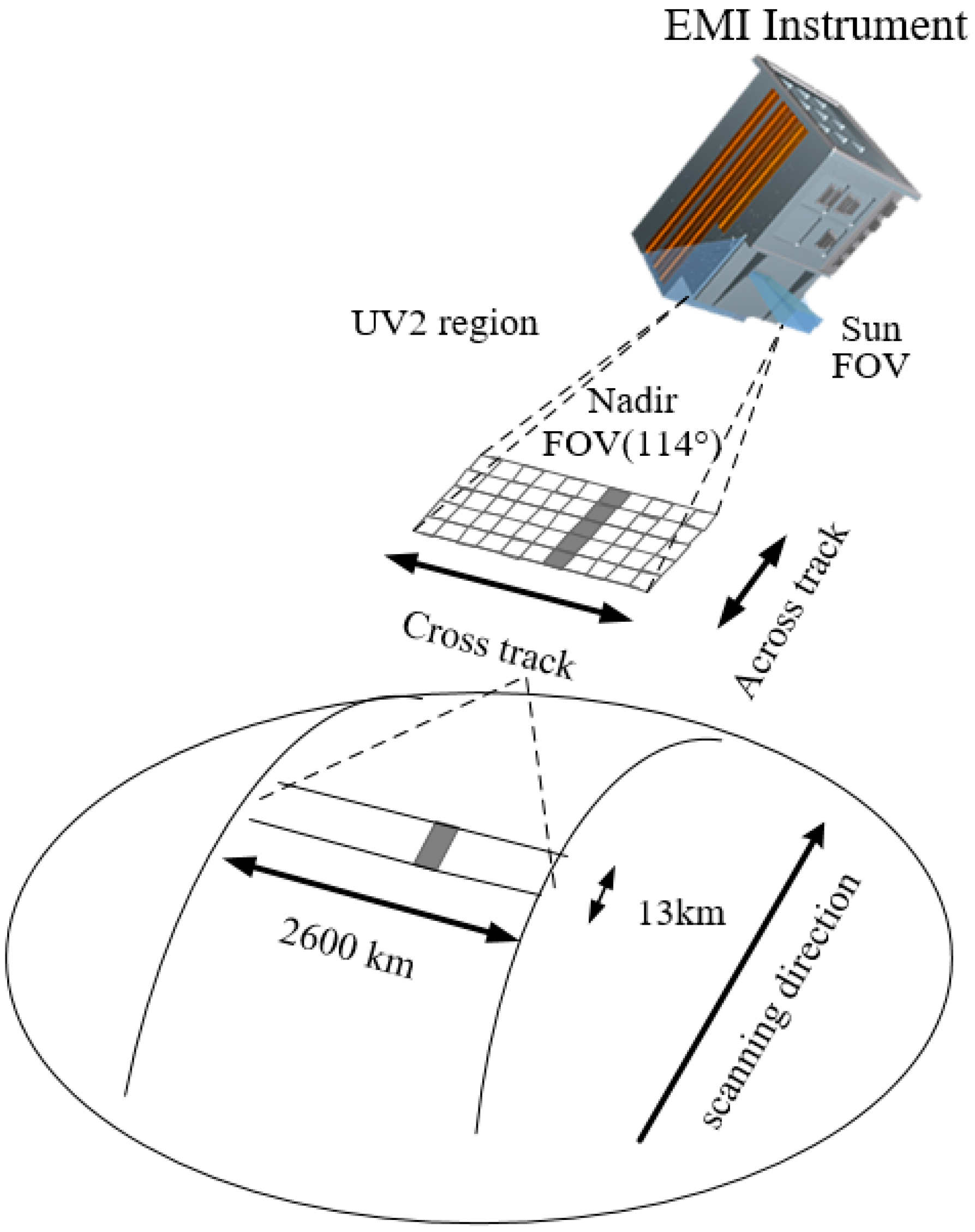
2.1. EMI Data
2.2. Auxiliary Data
3. EMI AAI Retrieval Algorithm
3.1. Calculation of the AAI
3.2. Calculation of the Contribution of a Cloud to the AAI
3.3. Look-Up Tables
3.4. Correction of AAI Errors
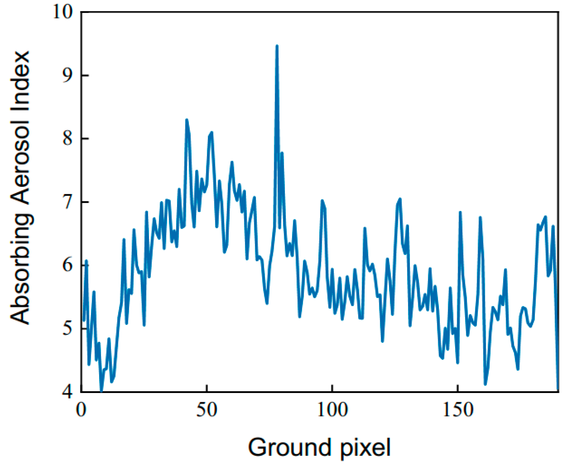
- We selected the window (50 along track × 191 across track pixels in size) with the minimum variance in AAI to ensure that the region did not entail any aerosol absorbing pollution.
- We calculated the average AAI value of 191 ground pixels in the scanline direction.
- We performed the Fourier analysis to determine the low and high frequencies of 191 average values. The high-frequency signals were interpreted as stripe noise, which can be subtracted from the initial AAI value along the track.
4. Results and Discussion
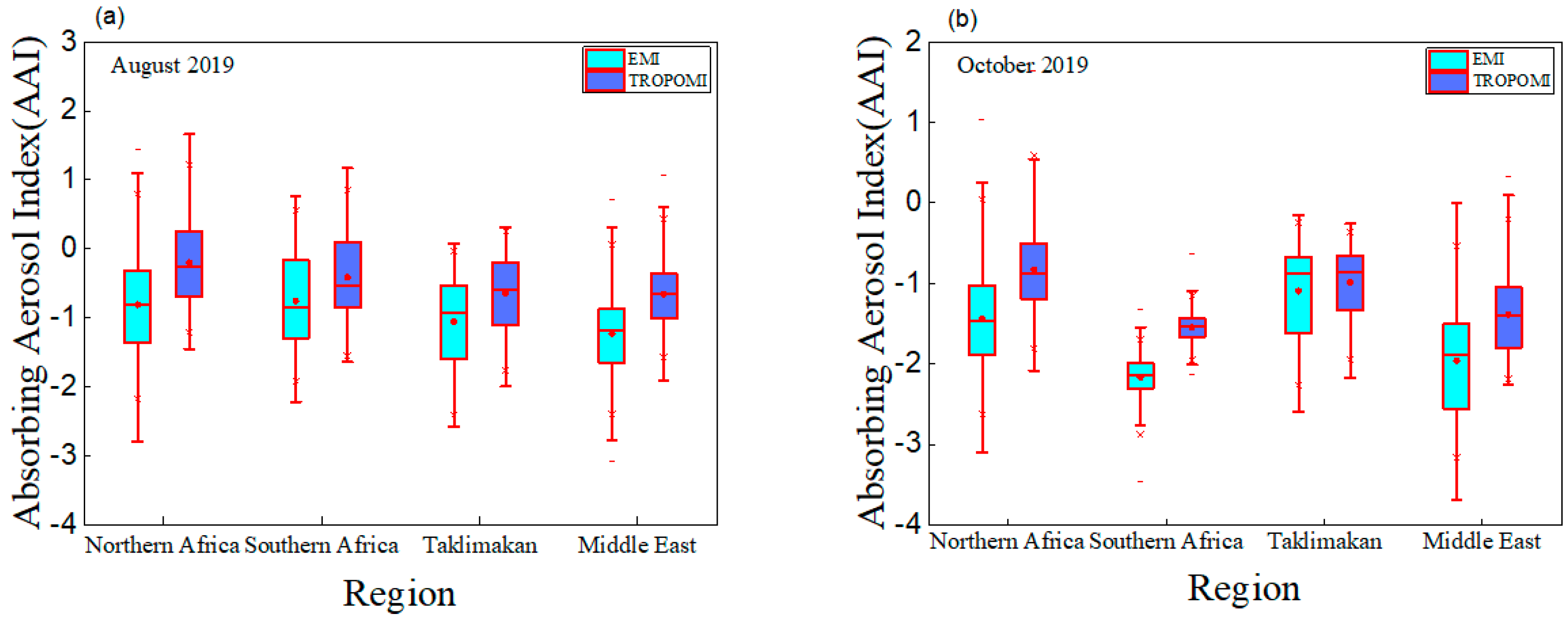
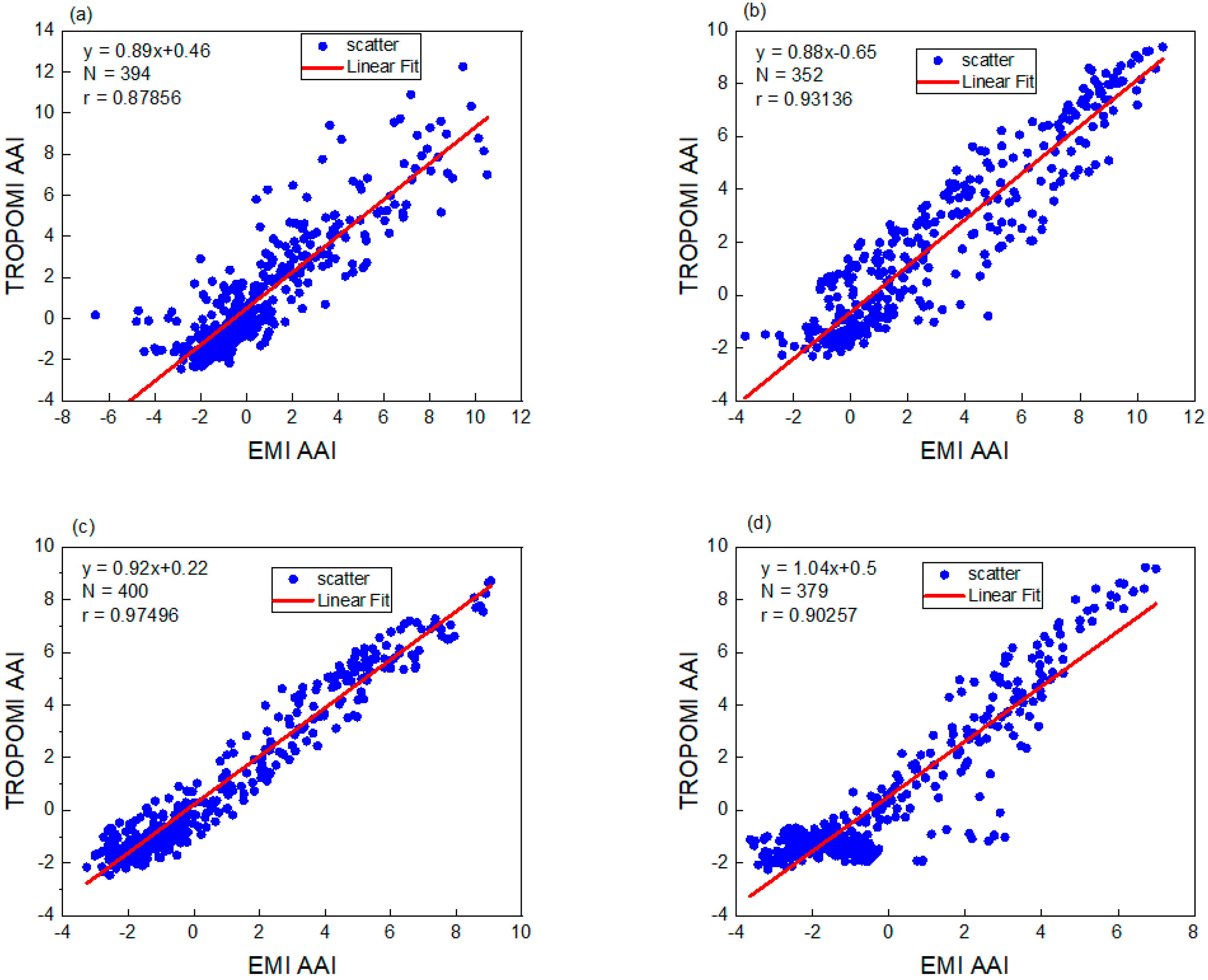
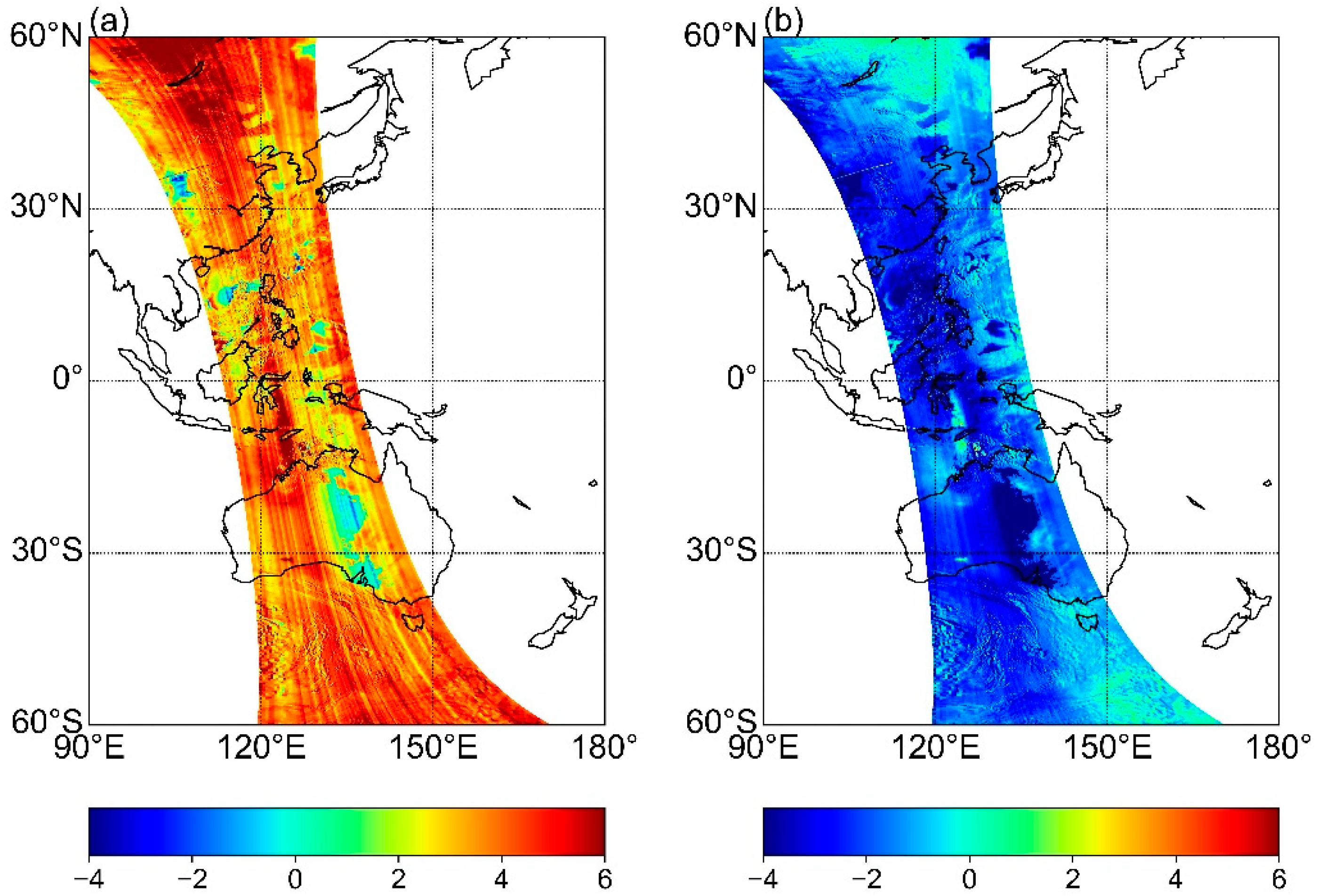
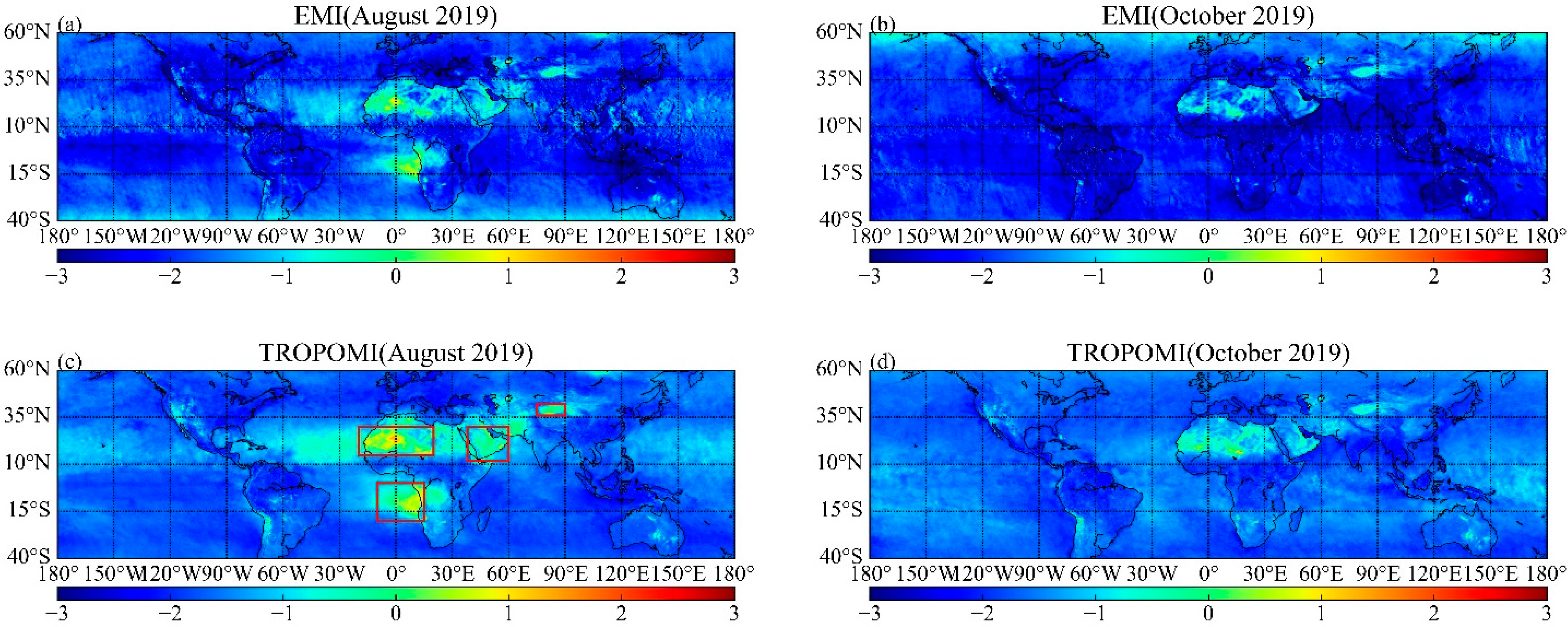
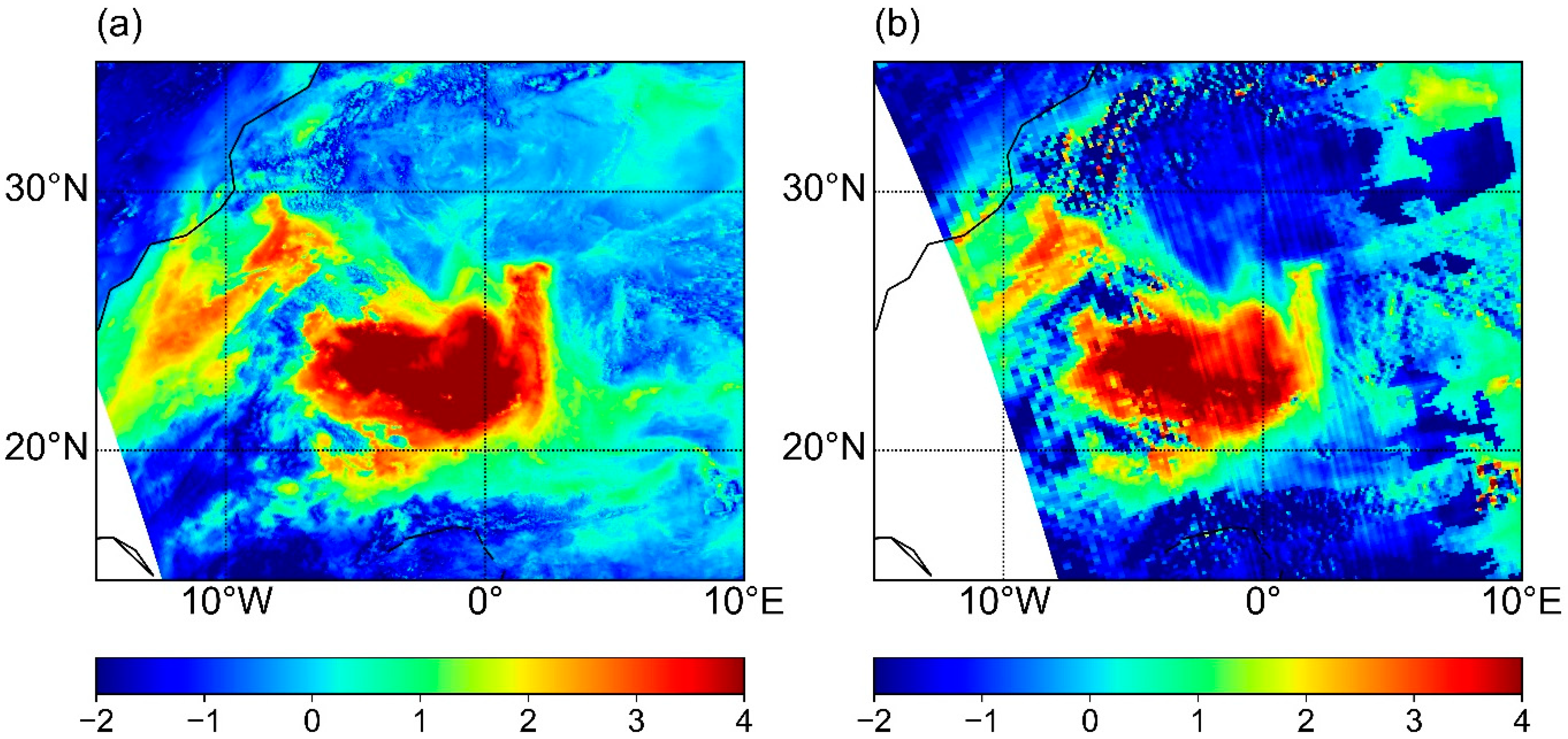
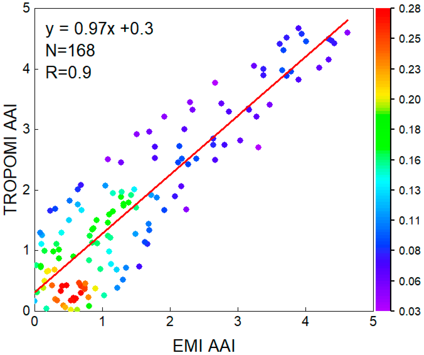
4.1. Comparison with TROPOMI AAI
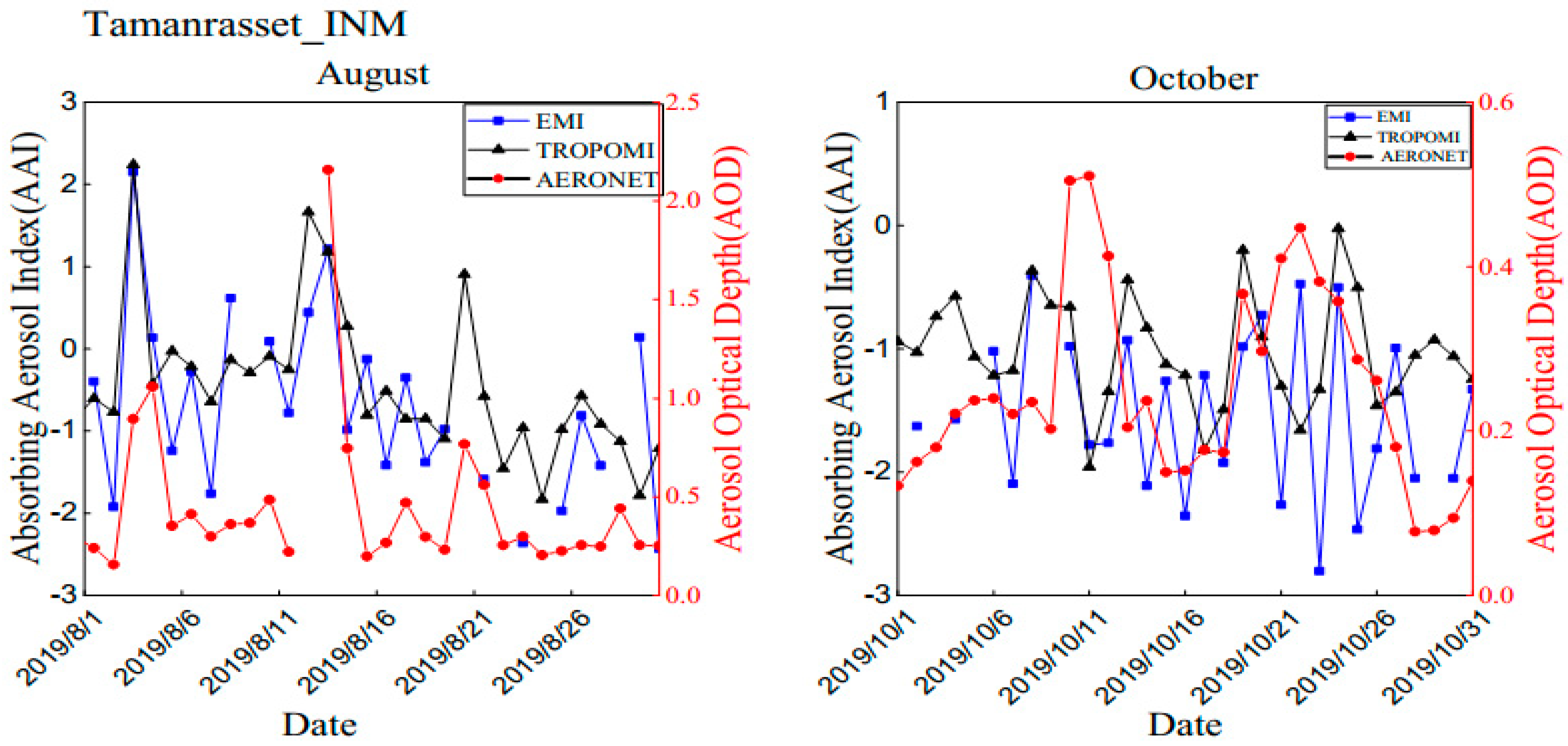
4.2. EMI versus AOD Measurements
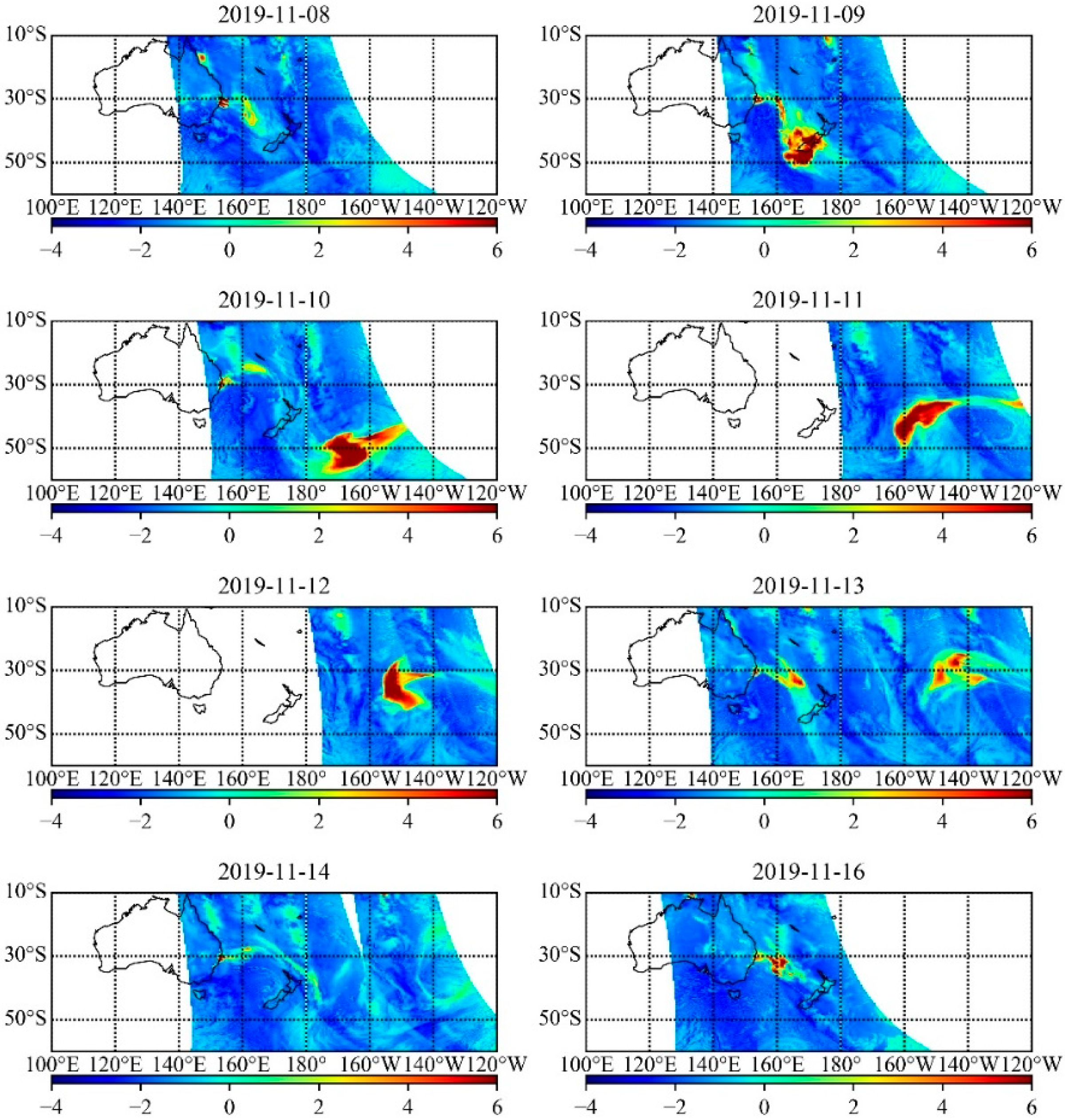
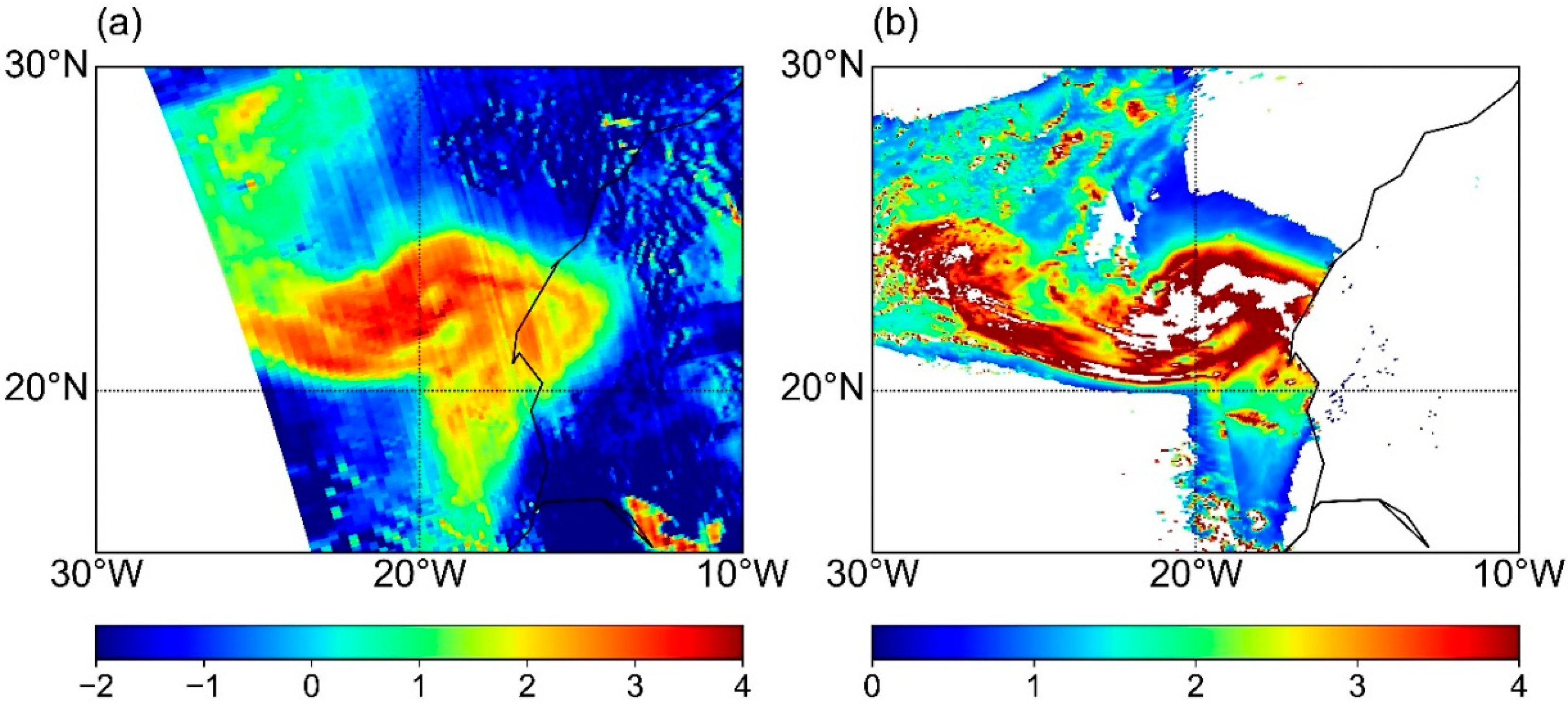
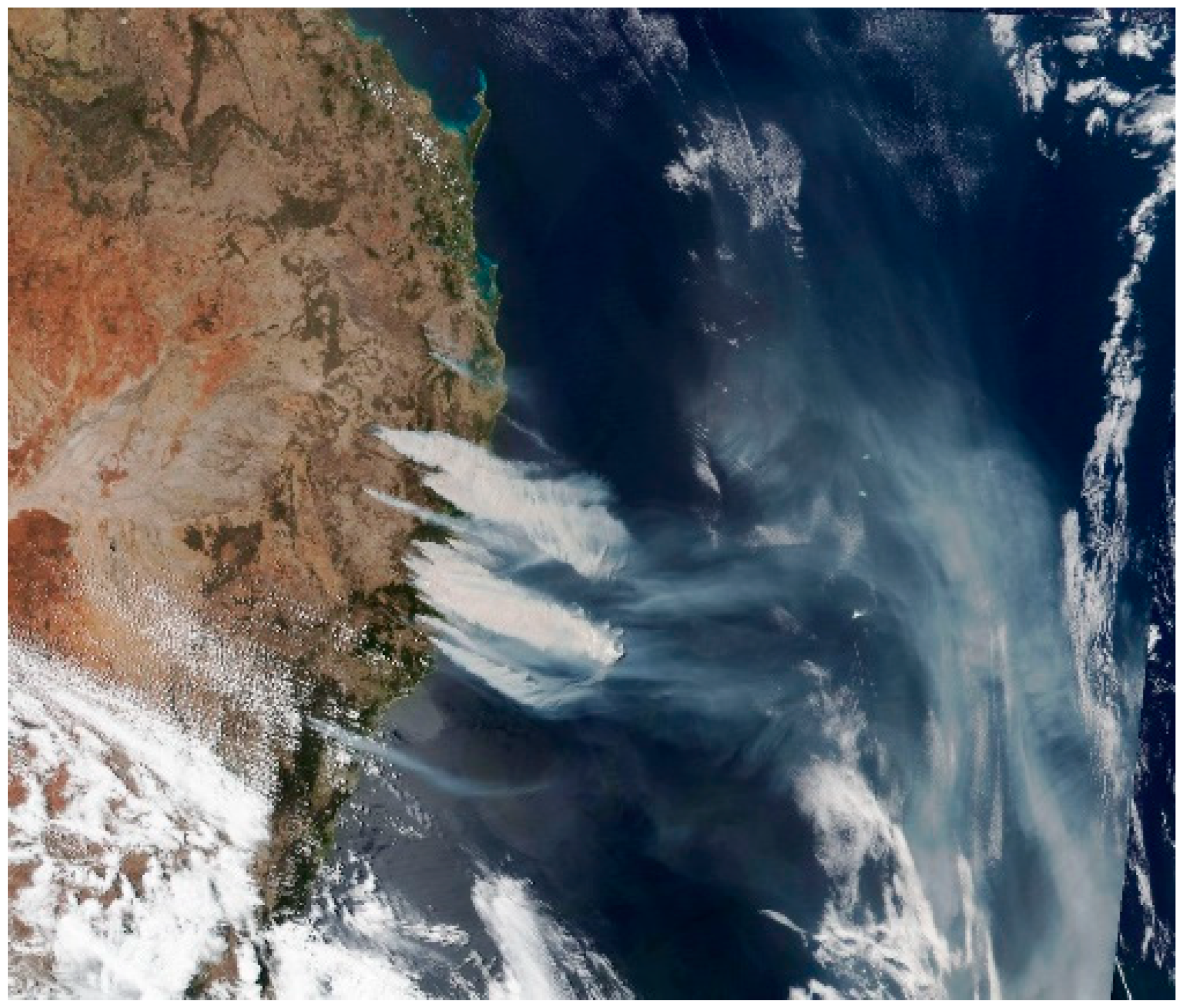
4.3. Case Study
5. Discussion and Conclusions
Author Contributions
Funding
Data Availability Statement
Acknowledgments
Conflicts of Interest
References
- Torres, O.; Bhartia, P.K.; Herman, J.R.; Sinyuk, A.; Ginoux, P.; Holben, B. A Long-Term Record of Aerosol Optical Depth from TOMS Observations and Comparison to AERONET Measurements. J. Atmos. Sci. 2002, 59, 398–413. [Google Scholar] [CrossRef]
- Torres, O.; Bhartia, P.K.; Herman, J.R.; Gleason, Z.A.J. Derivation of aerosol properties from satellite measurements of backscattered ultraviolet radiation: Theoretical basis. J. Geophys. Res. 1998, 103, 17099–17110. [Google Scholar] [CrossRef]
- Kaufman, Y.J.; Tanré, D.; Boucher, O. A satellite view of aerosols in the climate system. Nature 2002, 419, 215–223. [Google Scholar] [CrossRef] [PubMed]
- Satheesh, S.K.; Torres, O.; Remer, L.A.; Suresh Babu, S.; Vinoj, V.; Eck, T.F.; Kleidman, R.G.; Holben, B.N. Improved assessment of aerosol absorption using OMI-MODIS joint retrieval. J. Geophys. Res. 2009, 114, D05209. [Google Scholar] [CrossRef]
- Hsu, N.; Seftor, C.; Torres, O.; Eck, T.; Thompson, A.; Gleason, J.; Holben, B. Detection of Biomass Burning Smoke from TOMS Measurements. Geophys. Res. Lett. 1996, 23, 745–748. [Google Scholar] [CrossRef]
- Gleason, J.F.; Hsu, N.C.; Torres, O. Biomass burning smoke measured using backscattered ultraviolet radiation: SCAR-B and Brazilian smoke interannual variability. J. Geophys. Res. 1998, 103, 31969–31978. [Google Scholar] [CrossRef]
- Chiapello, I.; Prospero, J.M.; Herman, J.R.; Hsu, N.C. Detection of mineral dust over the North Atlantic Ocean and Africa with the Nimbus 7 TOMS. J. Geophys. Res. 1999, 104, 9277–9291. [Google Scholar] [CrossRef]
- Mahowald, N.M.; Dufresne, J.-L. Sensitivity of TOMS aerosol index to boundary layer 30 height: Implications for detection of mineral aerosol sources. Geophys. Res. Lett. 2004, 31, L03103. [Google Scholar] [CrossRef]
- Herman, J.R.; Bhartia, P.K.; Torres, O.; Hsu, C.; Seftor, C.; Celarier, E. Global distribution of UV-absorbing aerosols from nimbus 7/TOMS data. J. Geophys. Res. Atmos. 1997, 102, 16911–16922. [Google Scholar] [CrossRef]
- Hsu, N.; Herman, J.R.; Torres, O.; Holben, B.N.; Tanre, D.; Eck, T.F.; Smirnov, A.; Chatenet, B.; Lavenu, F. Comparisons of the TOMS aerosol index with Sun-photometer aerosol optical thickness: Results and applications. J. Geophys. Res. Atmos. 1999, 104, 6269–6279. [Google Scholar] [CrossRef]
- Alpert, P.; Ganor, E. Sahara mineral dust measurements from TOMS: Comparison to surface observations over the Middle East for the extreme dust storm, 14–17 March 1998. J. Geophys. Res. 2001, 106, 18275–18286. [Google Scholar] [CrossRef]
- Burrows, J.P.; Weber, M.; Buchwitz, M.; Rozanov, V.; Ladstatter-Weissenmayer, A.; Richter, A.; DeBeek, R.; Hoogen, R.; Bramstedt, K.; Eichmann, K.U.; et al. The global ozone monitoring experiment (gome): Mission concept and first scientific results. J. Atmos. Sci. 1999, 56, 151–175. [Google Scholar] [CrossRef]
- Tuinder, O.; Tilstra, G. Product User Manual for the NRT, Offline and Data Record Absorbing Aerosol Index Products. KNMI, ACSAF/KNMI/PUM/002, 2020, 1.91, 36. Available online: https://acsaf.org/docs/pum/Product_User_Manual_NAR_NAP_ARS_ARP_Apr_2020.pdf (accessed on 1 June 2022).
- Balzer, W.; Spurr, R.; Thomas, W.; Kretschel, K.; Bollner, M. SCIAMACHY Level 1b to 2 NRT Processing Input/Output Date Definition; Tech. Rep. ENV-TN-DLR-SCIA-0010; Issue 3/B, Deutsches Zentrum für Luft- und Raumfahrt: Oberpfaffenhofen, Germany, 2000. [Google Scholar]
- De Graaf, M.; Stammes, P. SCIAMACHY Absorbing Aerosol Index—Calibration issues and global results from 2002–2004. Atmos. Chem. Phys. 2005, 5, 2385–2394. [Google Scholar] [CrossRef]
- Penning de Vries, M.J.M.; Beirle, S.; Wagner, T. UV Aerosol Indices from SCIAMACHY: Introducing the SCattering Index (SCI). Atmos. Chem. Phys. 2009, 9, 9555–9567. [Google Scholar] [CrossRef]
- Buchard, V.; da Silva, A.M.; Colarco, P.R.; Darmenov, A.; Randles, C.A.; Govindaraju, R.; Torres, O.; Campbell, J.; Spurr, R. Using the OMI aerosol index and absorption aerosol opticaldepth to evaluate the NASA MERRA Aerosol Reanalysis. Atmos. Chem. Phys. 2015, 15, 5743–5760. [Google Scholar] [CrossRef]
- Levelt, P.F.; Joiner, J.; Tamminen, J.; Veefkind, J.P.; Bhartia, P.K.; Stein Zweers, D.C.; Duncan, B.N.; Streets, D.G.; Eskes, H.; van der A, R.; et al. The ozone monitoring instrument: Overview of 14 years in space. Atmos. Chem. Phys. 2018, 18, 5699–5745. [Google Scholar] [CrossRef]
- Sun, J.; Veefkind, J.P.; Velthoven, P.V.; Levelt, P.F. Quantifying the single scattering albedo for the January 2017 Chile wildfires from simulations of the OMI absorbing aerosol index. Atmos. Meas. Tech. 2018, 11, 5261–5277. [Google Scholar] [CrossRef]
- Kooreman, M.L.; Stammes, P.; Trees, V.; Sneep, M.; Tilstra, L.G.; de Graaf, M.; Stein Zweers, D.C.; Wang, P.; Tuinder, O.N.E.; Veefkind, J.P. Effects of clouds on the UV Absorbing Aerosol Index from TROPOMI. Atmos. Meas. Tech. 2020, 13, 6407–6426. [Google Scholar] [CrossRef]
- Veefkind, J.P.; Aben, I.; McMullan, K.; Förster, H.; de Vries, J.; Otter, G.; Claas, J.; Eskes, H.J.; de Haan, J.F.; Kleipool, Q.; et al. TROPOMI on the ESA sentinel-5 precursor: A GMES mission for global observations of the atmospheric composition for climate, air quality and ozone layer applications. Remote Sens. Environ. 2012, 120, 70–83. [Google Scholar] [CrossRef]
- Cheng, L.; Tao, J.; Valks, P.; Yu, C.; Liu, S.; Wang, Y.; Xiong, X.; Wang, Z.; Chen, L. NO2 Retrieval from the Environmental Trace Gases Monitoring Instrument (EMI): Preliminary Results and Intercomparison with OMI and TROPOMI. Remote Sens. 2019, 11, 3017. [Google Scholar] [CrossRef]
- Qian, Y.; Luo, Y.; Si, F.; Zhou, H.; Yang, T.; Yang, D.; Xi, L. Total Ozone Columns from the Environmental Trace Gases Monitoring Instrument (EMI) Using the DOAS Method. Remote Sens. 2021, 13, 2098. [Google Scholar] [CrossRef]
- Penning, D.; Wagner, T. Modelled and measured effects of clouds on UV Aerosol Indices on a local, regional, and global scale. Atmos. Chem. Phys. 2010, 10, 12715–12735. [Google Scholar]
- De Graaf, M.; Stammes, P.; Torres, O.; Koelemeijer, R.B.A. Absorbing Aerosol Index—Sensitivity analysis, application to GOME and comparison with TOMS. J. Geophys. Res. 2005, 110, D01202. [Google Scholar] [CrossRef]
- Holben, B.N.; Eck, T.; Slutsker, I.; Tanre, D.; Buis, J.P.; Setzer, A.; Vermote, E.; Reagon, J.A.; Kaufman, Y.J.; Nakajima, T.; et al. AERONET—A federated instrument network and data archive for aerosol characterization. Remote Sens. Environ. 1998, 66, 1–16. [Google Scholar] [CrossRef]
- Marshak, A.; Davis, A.; Wiscombe, W.; Titov, G. The verisimilitude of the independent pixel approximation used in cloud remote sensing. Remote Sens. Environ. 1995, 52, 71–78. [Google Scholar] [CrossRef]
- Koelemeijer, R.B.A.; Stammes, P.; Hovenier, J.W.; de Haan, J.F. A fast method for retrieval of cloud parameters using oxygen a band measurements from the global ozone monitoring experiment. J. Geophys. Res. Atmos. 2001, 106, 3475–3490. [Google Scholar] [CrossRef]
- Wang, P.; Stammes, P.; van der, A.R.; Pinardi, G.; van Roozendael, M. FRESCO+: An improved O2 A-band cloud retrieval algorithm for tropospheric trace gas retrievals. Atmos. Chem. Phys. 2008, 8, 6565–6576. [Google Scholar] [CrossRef]
- Rozanov, V.V.; Buchwitz, M.; Eichmann, K.-U.; de Beek, R.; Burrows, J.P. SCIATRAN—A new radiative transfer model for geophysical applications in the 240–2400 nm spectral region: The pseudo-spherical version. Adv. Space Res. 2002, 29, 1831–1835. [Google Scholar] [CrossRef]
- Zhang, C.X.; Liu, C.; Chan, K.L.; Hu, Q.H.; Liu, H.R.; Li, B.; Xing, C.Z.; Tan, W.; Zhou, H.J.; Si, F.Q.; et al. First observation of tropospheric nitrogen dioxide from the environmental trace gases monitoring instrument onboard the Gaofen-5 satellite. Light Sci. Appl. 2020, 9, 66. [Google Scholar] [CrossRef]
- Zhao, M.J.; Si, F.Q.; Zhou, H.J.; Wang, S.M.; Jiang, Y.; Liu, W.Q. Preflight calibration of the Chinese environmental trace gases monitoring instrument (EMI). Atmos. Meas. Tech. 2018, 11, 5403–5419. [Google Scholar] [CrossRef]
- Stein Zweers, D.C. TROPOMI ATBD of the UV Aerosol Index; Document Number—S5P-KNMI-L2-0008-RP; CI-7430-ATBD_UVAI; KNMI: De Bilt, The Netherlands, 2018; 30p. [Google Scholar]
- Ludewig, A.; Kleipool, Q.; Bartstra, R.; Landzaat, R.; Leloux, J.; Loots, E.; Meijering, P.; van der Plas, E.; Rozemeijer, N.; Vonk, F.; et al. In-flight calibration results of the TROPOMI payload on board the Sentinel-5 Precursor satellite. Atmos. Meas. Tech. 2020, 13, 3561–3580. [Google Scholar] [CrossRef]
- Boersma, K.F.; Eskes, H.J.; Veefkind, J.P.; Brinksma, E.J.; van der A, R.J.; Sneep, M.; van den Oord, G.H.J.; Levelt, P.F.; Stammes, P.; Gleason, J.F.; et al. Near-real time retrieval of tropospheric NO2 from OMI. Atmos. Chem. Phys. 2007, 7, 2103–2118. [Google Scholar] [CrossRef]
- Duncan, B.N.; Martin, R.V.; Staudt, A.C.; Yevich, R.; Logan, J.A. Interannual and seasonal variability of biomass burning emissions constrained by satellite observations. J. Geophys. Res. 2003, 108, 4100. [Google Scholar] [CrossRef]


| Parameter | Node |
|---|---|
| SZA (°) | 0.1, 10.0, 20.0, 30.68, 40.54, 45.57, 50.21, 55.94, 60.0, 65.17, 70.12, 72.54, 74.93, 76.11, 80.79, 84.26 |
| VZA (°) | 0.1, 10.0, 20.0, 30.68, 40.54, 45.57, 50.21, 55.94, 60.0, 65.17, 70.12 |
| RAA (°) | 0, 30, 60, 90, 120, 150, 180 |
| Surface altitude/Cloud height (km) | 0, 0.2, 0.4, 0.8, 1.2, 1.6, 2.0, 2.4, 2.8, 3.2, 3.6, 4.0, 4.6, 5.0, 5.6, 6.2, 7.0, 8.0, 9.0, 10.0, 12.0, 14.0 |
| Monthly | August | October | |||
|---|---|---|---|---|---|
| Region | r | RMSE | r | RMSE | N |
| Northern Africa | 0.92 | 0.67 | 0.92 | 0.66 | 4800 |
| Southern Africa | 0.93 | 0.43 | 0.55 | 0.65 | 4000 |
| Middle East | 0.91 | 0.61 | 0.92 | 0.64 | 3168 |
| Taklimakan | 0.94 | 0.47 | 0.90 | 0.27 | 720 |
Publisher’s Note: MDPI stays neutral with regard to jurisdictional claims in published maps and institutional affiliations. |
© 2022 by the authors. Licensee MDPI, Basel, Switzerland. This article is an open access article distributed under the terms and conditions of the Creative Commons Attribution (CC BY) license (https://creativecommons.org/licenses/by/4.0/).
Share and Cite
Tang, F.; Wang, W.; Si, F.; Zhou, H.; Luo, Y.; Qian, Y. Successful Derivation of Absorbing Aerosol Index from the Environmental Trace Gases Monitoring Instrument (EMI). Remote Sens. 2022, 14, 4105. https://doi.org/10.3390/rs14164105
Tang F, Wang W, Si F, Zhou H, Luo Y, Qian Y. Successful Derivation of Absorbing Aerosol Index from the Environmental Trace Gases Monitoring Instrument (EMI). Remote Sensing. 2022; 14(16):4105. https://doi.org/10.3390/rs14164105
Chicago/Turabian StyleTang, Fuying, Weihe Wang, Fuqi Si, Haijin Zhou, Yuhan Luo, and Yuanyuan Qian. 2022. "Successful Derivation of Absorbing Aerosol Index from the Environmental Trace Gases Monitoring Instrument (EMI)" Remote Sensing 14, no. 16: 4105. https://doi.org/10.3390/rs14164105
APA StyleTang, F., Wang, W., Si, F., Zhou, H., Luo, Y., & Qian, Y. (2022). Successful Derivation of Absorbing Aerosol Index from the Environmental Trace Gases Monitoring Instrument (EMI). Remote Sensing, 14(16), 4105. https://doi.org/10.3390/rs14164105