Abstract
Plastic mulch is extensively applied in agricultural production in arid regions. It significantly influences the interactions between land and atmosphere by altering underlying surface characteristics. An accurate and timely extraction method for Plastic-Mulched Cropland (PMC) is required to understand land surface energy transfer processes, eco-hydrological cycle, the climate effect of PMC, and in the management of water resources. In this study, we proposed a Timely Plastic-mulched cropland Extraction Method (TPEM) from complex mixed surfaces with multi-source remote sensing data in the Shiyanghe River Basin (SRB), a typical representation of a complex and inhomogeneous arid region in the northwest of China. We defined TPEM in three phases; in the first phase, the spectral characteristic curves were drawn from ground object points labeled by visual interpretation with multi-source remote sensing data. In the second phase, a spectral characteristic analysis of the modified index was proposed to amplify the difference between PMC and non-PMC ground objects. Finally, the Classification and Regression Tree (CART) classifier was used to generate thresholds of indices as PMC extraction rules. The results showed that it can extract the boundary of PMC in large-scale farmland, distinguish PMC from ground objects in complex mixed surfaces, and separate the PMC from desert land that shares same spectral characteristics with PMC. The TPEM is verified to be efficient and robust, with an overall accuracy of 0.9234, quantity disagreement of 0.0541, and allocation disagreement of 0.0224, and outperformed two extensively used PMC extraction methods, especially for timely PMC extraction when satellite data only during the period that ground surface incomplete covered by plastic mulch is available. This study will provide us with an accurate and timely method to extract PMC, especially in the widely distributed complex mixed surfaces.
1. Introduction
Plastic mulch has been used extensively in the arid and semi-arid areas in China since the end of the 20th century due to its ability to reduce soil evaporation, increase soil temperature, and promote crop yields [1,2,3]. However, plastic mulch alters the surface albedo and influences the energy and water transfer processes between the underlying surface and atmosphere, further affecting regional climate [4]. Moreover, wide application of plastic mulch will also cause environmental issues if it is not properly removed after use or degraded in natural conditions [5,6]. The crop yield will decrease significantly when residual plastic mulch exceeds 240 kg/ha [7]. It is essential to know the distribution of Plastic-Mulched Cropland (PMC) to accurately evaluate the mulching effect on the local climate and the residual contamination caused by the extensive plastic mulch application. However, collected statistics about plastic mulch (the collected statistics more focus on the usage or the area of PMC rather than the distribution of the PMC) are based on administrative areas rather than natural basins. The administrative regions and natural basins are often inconsistent, introducing errors in the usage or the area of the PMC.
Remote sensing technology, which can be used to extract ground surface information efficiently, is also a good method to extract PMC information. Some studies [8,9,10,11] are based on the local computing software such as ENVI to extract the PMC. Lu et al. [8] first generated a decision-tree classifier, and the result implies that the classifier is temporarily stable to be applied in different years. Then, a threshold model for detecting transparent film mulch was proposed using Landsat 5 Thematic Mapper (TM) to map PMC over a large geographic area [9] but cannot extract PMC accurately in other regions during tests. Moreover, an Object-Based Image Analysis (OBIA) approach [10] was proposed using Sentinel-1 SAR and Sentinel-2 data. Three machine-learning algorithms, including classification and regression tree (CART) [12], Random Forest (RF) [13,14], and Support Vector Machines (SVM) [15], were carried out. The results showed that the SVM and RF classifiers performed better than the CART classifier in the Overall Accuracy (OA) and kappa accuracy in most cases. Hasituya and Chen [11] gathered the spectra, textures, and thermal features into RF and SVM machine-learning algorithms. They found that NDVI, Greenness Index (GI), and textural features of the mean are more critical than the other features for mapping PMC in Jizhou, during April and May, because both months are optimal periods for mapping PMC in Jizhou. These studies require collecting large amounts of remote sensing image data and are slow to compute locally. Some studies based on the cloud computing platforms Google Earth Engine (GEE) for data processing improve computation speed and reduce costs. Hao et al. [16] proposed a new workflow merging PMC of multiple temporal phases using Sentinel-2 data of Hengshui, China, and have good potential to identify PMC in Guyuan, China. Xiong et al. [17] detected PMC in Xinjiang, China using multi-temporal and multi-sensor satellite images with a CART classifier, and an overall accuracy of 92.2% for the PMC. All the above studies cannot provide a method with simple format as well as accurately and timely PMC extraction results at the same time.
Accurate and timely PMC extraction from complex mixed underlying surfaces requires a more effective index to (1) distinguish PMC from ground objects that share similar spectral characteristics, (2) raise the PMC extraction method’s accuracy, and (3) reduce the requirement for remote sensing data. However, great challenges still exist. First, considering the PMC has the same spectral characteristics as sand and impervious surfaces, neither plastic mulch index can distinguish these ground objects easily. Second, most farmlands in China are usually distributed separately in anthropic regions, raising difficulties in classification of ground objects over complex mixed underlying surfaces. Third, the requirement of having satellite data for long periods, that extend from seeding to growing periods, limit the application of previous methods in timely extraction of PMC distribution [8,17]. Therefore, the main objectives of this study are: (1) to propose a timely PMC extraction method (TPEM) to obtain the plastic-mulched croplands distribution accurately and quickly by modifying a remote sensing index through amplifying the difference between PMC and other ground objects; (2) to verify the TPEM in a typical complex mixed underlying surfaces region, the Shiyanghe River Basin, only using data for the plastic mulch just being applied, without being covered by plants.
2. Materials and Methods
2.1. Study Area
The Shiyanghe River Basin (SRB) was chosen as the study area because it belongs to an arid region and plastic mulch is widely used in this region. Mainly located in the Gansu Province in northwest China, as shown in Figure 1, this basin extends from 36°29′ to 39°27′N and from 101°22′ to 104°16′E, with an area of 41,600 km2 [18,19]. The underlying surface in the SRB is complex, with the fragmentary cropland interspersed with urban impervious surface, which can represent the most of croplands in China. On the one hand, plastic mulch used in the SRB can maintain soil moisture, promote crop growth, and increase crop yield [20,21]. On the other hand, the residual plastic mulch can contaminate the soil, reducing crop yield. It has an annual precipitation of only 164 millimeter (mm), belonging to the arid climate, with mean annual pan evaporation of 2000 mm [22]. The plastic mulch was used in this basin to best use the scarce water resources and increase the local grain yield with a severe water resource shortage. The widespread use of plastic mulch in the SRB will alter the surface albedo and influence the energy and water exchange between the ground surface and atmosphere [4]. Thus, to estimate this influence, it is necessary to know the distribution of local PMC.
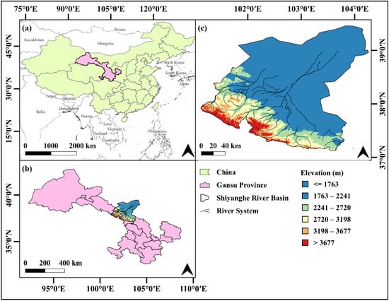
Figure 1.
Location and elevation maps of the SRB. (a) The position of China and Gansu province in China’s provincial administrative regions. (b) the location of SRB in the Gansu province municipal administrative region. The area of SRB includes several municipal districts. (c) the boundary, elevation map, and river system of the SRB.
In the SRB, there are two main deserts, Badain Jaran Desert in the north and Tengger Desert in the east. It is hard to distinguish the sand from PMC because they share similar reflectance values in the visible band, which will overestimate the occurrence of PMC area [23,24]. Like most parts of China, the farmland is fragmentary and interlaced with urban impervious surfaces. This complex mixed surface contributes to the difficulty in PMC extraction.
2.2. Datasets
2.2.1. Satellites Data
In the satellite remote sensing data, the best time window to extract plastic mulch is during the period from the plastic mulch applied on the farmland to the crop canopy fully covered the ground surface. Considering the plastic mulch covered farmland will be sheltered by crop leaves as the plants growing up, the remote sensing data within the time window is crucial to PMC extraction. Hu et al. [25] mentioned the main crops in the SRB are wheat, corn, oil sunflower, and capsicum, which coincides with Gansu Province’s Agricultural Statistical Yearbook’s data [26]. According to Hu’s research [25], the seeding period varies from mid-March to mid-April. Then the plastic mulch will be gradually covered by crops within a month.
The remote sensing data for 2020 was chosen to propose the TPEM and build its extraction rules because in the time window of this year (from 1 April to 15 April), the PMC is clearly exposed to the satellite and be easily identified, which is helpful to obtain spectral characteristics. To apply this method to extract PMC in 2011–2021, the remote sensing data in time windows for these years need to be selected. Considering different years, the seeding periods as well as the time windows change with the solar term, and the calendar dates of solar term are not unique in each year. The data from 1 February to 31 July in each year were chosen to apply the TPEM proposed by this study. This time span can ensure the time windows of major crop be included. Due to the influence of clouds and the coarse temporal resolution of medium and high-resolution remote sensing images, it is impossible to fully cover the whole SRB only using a single source of remote sensing data. Thus, it is necessary to use multi-source remote sensing data to cover the whole SRB.
This study consists of four satellites including Sentinel-2 Multispectral Images (MSI), Landsat 8 Operational Land Images (OLI), Landsat 7 Enhanced Thematic Mapper Plus (ETM+), and Terra MODIS (Moderate-resolution Imaging Spectroradiometer). There are only six common bands including visible bands (Blue, Green, Red), NIR band, and SWIR1 and SWIR2 bands existing in these four satellites. The dataset of the MSI is from Leverl-2A, which is provided by European Space Agency (ESA, last accessed date: 8 December 2021 (https://sentinel.esa.int/web/sentinel/user-guides/sentinel-2-msi/product-types/level-2a)). The dataset from MSI have 10 meter’s spatial resolution in the Blue, Green, Red, and NIR bands and have 20 meter’s spatial resolution in the SWIR1 and SWIR2 bands. The dataset of OLI is in Level 2, which is provided by United States Geological Survey (USGS) (last accessed date: 8 December 2021, (https://www.usgs.gov/landsat-missions/landsat-surface-reflectance)). The dataset of OLI has 30 meter’s spatial resolution in the Blue, Green, Red, NIR, SWIR1, and SWIR2 bands. The dataset of ETM+ is in Level 2, which is provided by USGS (last accessed date: 8 December 2021; (https://www.usgs.gov/landsat-missions/landsat-surface-reflectance)). The dataset from ETM+ has 30 meters of spatial resolution in six common bands. The three products mentioned above can provide relatively clear images that can be used to obtain ground truth. The dataset of MODIS is MOD09A1 product, which is provided by National Aeronautics and Space Administration (NASA) (last accessed date: 8 December 2021, (https://lpdaac.usgs.gov/products/mod09a1v006/)). The dataset of MODIS has 500 meter’s spatial resolution in the six common bands, which means the ground truth cannot be identified by this product due to the coarser resolution. All the four datasets are surface reflectance products and can be downloaded, used, and processed by GEE platform.
This study used remote sensing images from the seeding period to propose mPMCI (modified plastic-mulched cropland index). In addition, four data sources were mixed and used to reduce the influence of clouds. Considering these four data sources have different time availabilities, Table 1 shows which satellite data sources were used in the different periods.

Table 1.
The remote sensing datasets used for proposing TPEM.
2.2.2. Ground Truth
In the SRB, the main ground objects include PMC, vegetation, impervious surface, sand, farmland, snow, and water. In this study, we used 4456 sample points. These sample points presenting ground truth were randomly selected and then labeled by visual interpretation to display the spectral characteristic, train the machine-learning-based classifiers, and evaluate the effectiveness of the PMC extraction rules generated by the classifiers. To focus on the PMC extraction, other ground objects except PMC were classed as non-PMC. The classes and number of points of each class and final classes are shown in Table 2.
Table 2.
The main ground objects of the SRB and the number of sample points of these objects. Considering this study’s key is plastic-mulched cropland extraction, objects were classed together as non-PMC except for PMC.
This study also randomly selected and then labeled another isolated dataset to increase the objectivity and independence including 1035 points of PMC and 1484 points of non-PMC, to evaluate and compare the extraction accuracy of the TPEM and method proposed by other studies. All of these sample points can represent the ground truth.
2.2.3. Ancillary Data
To obtain the distribution and total area of farmland in the SRB, the cropland layer from the Finer Resolution Observation and Monitoring-Global Land Cover (FROM-GLC, last accessed date: 17 August 2021. Link: http://data.ess.tsinghua.edu.cn/) [27,28,29], which was a 30 m resolution global land cover map was used. The ratio of PMC to total farmland was calculated based on this product. Two versions of FROM-GLC data were selected considering farmland distribution and area change. Table 3 shows the file record and the other information of this dataset in detail.
Table 3.
The record of the FROM-GLC used in this study.
2.3. Method
A complete set of workflows was used in this study. The whole process can be divided into four parts, i.e., (1) data processing, (2) spectral characteristic extraction and analysis, (3) extraction rule generating, and (4) accuracy assessment. The workflow chart can be seen in Figure 2.
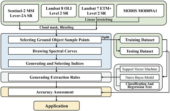
Figure 2.
The workflow chart shows how this study processed data, developed indices, and generated plastic-mulched farmland extraction rules in details.
First, the remote sensing satellite images of the SRB during the seeding period were filtered in the data processing. The Quality Assessment (QA) bands were used to remove the pixel covered by clouds or the shadow of clouds. A pixel where QA is equal to a certain value is seen as clouds or the shadow of clouds. The GEE platform provides a cloud removing function for every dataset [30,31,32,33]. However, this function will mask out the pixel covered by clouds and makes this pixel have no data. Therefore, this study used four satellite datasets and blended them to reduce the data loss caused by cloud removal. The detail of this part is introduced in Section 2.3.1.
For the spectral characteristic extraction and analysis, this study first selected ground object sample points using visual interpretation and split them into training and testing datasets. Then the spectral curves of these seven types of ground objects were drawn to analyze their spectral characteristics. The details of this part is introduced in Section 2.3.2.
This study used a machine-learning algorithm CART [12] with a modified plastic mulch index to generate the TPEM in the extraction rule generating part. The details of this part are introduced in Section 2.3.3. Finally, the accuracy assessment method is introduced in Section 2.3.4.
2.3.1. Multi-Source Data Fusion
The available remote sensing images are rare to extract plastic mulch from the plastic mulch applied on the farmland to the crop canopy fully covered with mulch. Considering the medium and high-resolution remote sensing images usually have coarse temporal resolution and there is only a short time window. After using the clouds removing function, the pixel covered by the clouds and shadow of clouds will be removed and only left a hole without remote sensing data. Therefore, it is impossible to cover the whole basin only using a single remote sensing data source. Luckily, the MSI and OLI have good consistency in the plastic-covered agriculture area [34]. Thus, this study used multi-source remote sensing data to fix the data hole. The data from MSI was selected as the first layer. It has the highest resolution among these four satellite datasets. The second layer was the data from OLI, and the third layer was ETM+. These two datasets have a lower resolution at 30 m, and considering ETM+ had scanner error since 31 May 2003; this dataset was put in the third layer. However, even blending these three satellites datasets cannot make sure there are no holes left. Therefore, the data from MODIS was selected as the bottom layer. The 500 m resolution of it can barely not be used to show the feature of the ground object, but this dataset was composited over fifteen days, so almost no clouds exist. Considering the four datasets is not all available during 2011–2021, some datasets cannot provide data before a specific time, as seen in Table 1. For example, the data from MSI is not available before 28 March 2017. In this situation, the first layer is not available and blend the remaining datasets in order.
The discrepancies in different sensors would affect the combination of these datasets. For example, the root means square error (RMSE) is more significant than 8% in the red band between MSI and ETM+ data [35]. This study used a relevant linear model [36,37] to eliminate the discrepancies between different sensors. Based on the data from MSI, this linear model calibrated the data from OLI, ETM+, and MODIS to be consistent with the data from MSI.
Taking MSI and ETM+ as an example to build up these relevant linear models, 165 sample points were picked from the globally overlapped areas of MSI and OLI at the same time. Then, with the reflectance of MSI as the vertical axis and the reflectance of ETM+ as the horizontal axis, the reflectance scatter diagrams and their trend lines of blue, green, red, NIR, SWIR1, and SWIR2 bands were drawn in Figure 3. The linear relationship between MSI and OLI, and MSI and MODIS are shown in Figure 4 and Figure 5, respectively. Third, according to these linear relationships, the six bands of ETM+ mentioned before can be calibrated to be consistent with MSI In the same way, 174 common points of MSI and ETM+ at the same time were selected, and 152 common points of MSI and MODIS at the same time were selected to build the linear model.
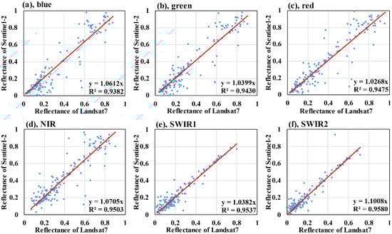
Figure 3.
Linear relationship between MSI and ETM+. The blue point is the reflectance of these two sensors and the red line is the linear fitting line. The first row is (a) blue band, (b) green band, and (c) red band from left to right, the second row is (d) near-infrared band, (e) short-wave infrared band type one, and (f) short-wave infrared band type two from left to right.
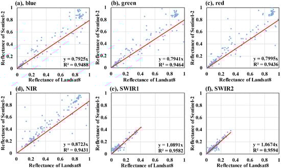
Figure 4.
Linear relationship between MSI and OLI. The blue point is the reflectance of these two sensors and the red line is the linear fitting line. The first row is (a) blue band, (b) green band, and (c) red band from left to right, the second row is (d) near-infrared band, (e) short-wave infrared band type one, and (f) short-wave infrared band type two from left to right.
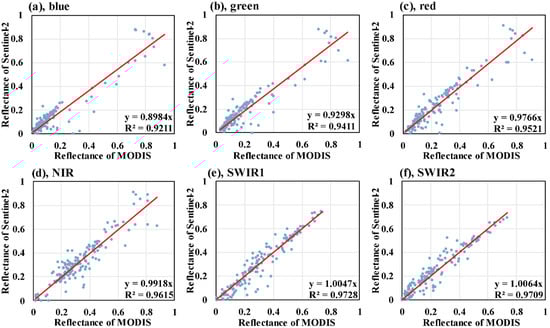
Figure 5.
Linear relationship between MSI and MODIS. The blue point is the reflectance of these two sensors and the red line is the linear fitting line. The first row is (a) blue band, (b) green band, and (c) red band from left to right, the second row is (d) near-infrared band, (e) short-wave infrared band type one, and (f) short-wave infrared band type two from left to right.
With these linear models, the cloud-removed remote sensing datasets can be calibrated to be consistent with MSI. Moreover, all the four datasets need to be resampled to 30m resolution due to different spatial resolutions. Finally, we blend these datasets to become the remote sensing dataset for this study.
2.3.2. Spectral Characteristic Extraction and Analysis
The ground truth points were labeled on the GEE platform using visual interpretation. Due to the spectral characteristics varying among different ground objects, these ground objects could represent different colors or features using the right combination of bands. Thus, they can be identified by the visual interpretation. Figure 6 shows the true color and false-color images of the SRB. The SRB’s seven main ground objects include PMC, vegetation, impervious surface, sand, farmland, snow, and water.
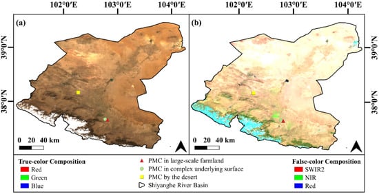
Figure 6.
(a) shows the true color (R = Red, G = green, B = blue) image and (b) shows the false-color (R = SWIR2, G = NIR, B = Red) image of the SRB, composed of MSI, OLI, ETM+, and MODIS from 1 April to 15 April 2020. The red triangle shows the PMC in large-scale farmland. The green circle shows the PMC in complex mixed surfaces. In addition, the yellow square shows PMC by the desert.
According to the ground truth sample points labeled using visual interpretation, the spectral reflectance curve was drawn by the GEE platform. As shown in Figure 7, different ground objects owned different reflectance curves. Take vegetation as an example. From visible bands (blue, green, and red bands) to near-infrared (NIR) bands, vegetation reflectance increased sharply to its highest value, which means the NIR band was sensitive to vegetation. This unique trend makes it possible to distinguish vegetation from other ground objects.
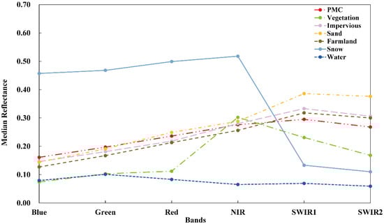
Figure 7.
Spectral reflectance curves of PMC, Vegetation, Impervious surface, Sand, Farmland, Snow, and Water. The reflectance value is the median value of sample points.
2.3.3. Modified Plastic Mulch Index and PMC Extraction Rules
Xiong et al. [17] proposed two PMFIs (plastic-mulched farmland index) based on the quotient of SWIR2 band and NIR band as well as the quotient of SWIR2 band and blue band. These two indices can be calculated as following Equations (1) and (2):
However, in the SRB, all ground objects between SWIR2 and NIR band are not as significant as the differences between SWIR1 and NIR band. Therefore, in this study, a modified plastic mulch index was proposed based on spectral characteristics. It is clear that PMC, impervious surface, sand, and farmland shared similar reflectance curves, but it can still be distinguished by targeted bands calculation. Although these four ground objects both show an increasing trend from blue band to SWIR1 band and get their peak at SWIR1 band then decrease, the trends of them from NIR to SWIR1 band are different. Based on this difference, the mPMCI was built up with the reciprocal normalization of the SWIR1 and NIR bands. The mPMCI can be calculated by the following Equation (3):
where is the reflectance of a pixel in the NIR band, is the reflectance of pixel in the SWIR1 band.
After building the mPMCI, setting a proper threshold is the simplest way to distinguish different ground objects. To figure out the threshold and build the extraction rules, this study tried three machine-learning-based classifiers: Support Vector Machines (SVM), Naive Bayesian Model (NBM) and CART, to train the sample points. The sample points fall into PMC or non-PMC. Then they were divided into two parts: the training part with randomly selected 70% sample points of each category to train the classifiers and the testing part with randomly selected 30% sample points of each category to test the classifiers and present classification results.
2.3.4. Accuracy Assessment
In essence, classification accuracy is typically taken to mean the degree to which the derived image classification agrees with reality or conforms to the truth. A classification error is some discrepancy between the situation depicted on the thematic map and reality [38]. In remote sensing image classification, the confusion matrix method is widely used to describe the relationship between the fundamental attribute of the sample data and the classification results. Based on the confusion matrix, some evaluation indices can be calculated. Overall accuracy (OA), quantity disagreement (QD), allocation disagreement (AD) [39], producer accuracy (PA), and user accuracy (UA) were used to assess classification accuracy of methods.
The following Equations (4)–(8) calculated these five indices:
where represents overall accuracy. is the proportion of the sample points that is category in the classification results and category in the real situation. represents quantity disagreement. represents allocation disagreement. and are producer accuracy and user accuracy of category g.
OA means the probability that the classification result is consistent with the actual type. QD is defined as the amount of difference between the reference map and a comparison map that is due to the less than perfect match in the proportions of the categories. AD is defined as the amount of difference between the reference map and a comparison map that is due to the less-than-optimal match in the spatial allocation of the categories [39]. PA means the probability of a pixel being correctly classified and UA implies the probability of a pixel classified on the map actually represents that category on the ground [40].
3. Results
3.1. PMC Extraction Rules
After choosing the remote sensing index and spectral band, the PMC can be extracted by setting thresholds of indices and bands. Points within the threshold range were identified as PMC. Three machine-learning-based algorithms were used to determine the thresholds efficiently. Taking classification accuracy as the evaluation standard, as Table 4 shows, the CART is best with 0.9157 of OA, 0.0112 of AD and 0.0731 of AD. The OA, QD and AD of SVM were 0.6709, 0.3037, and 0.0254, respectively. In addition, the OA, QD and AD of NBM were 0.2739, 0.3172, and 0.4090, which means this method is not suitable for the ground object classification. Moreover, the calculation speed of SVM is far slower than other methods during the actual operation, so the most suitable classifier is CART due to its high classification accuracy and high calculation speed. By repeatedly splitting the data into more homogeneous groups, CART has more advantages like ease of interpretation, comfort, and robustness of construction [41].
Table 4.
The performance of the three classifiers, overall accuracy, quantity disagreement, and allocation disagreement, were considered indicators because they reflect the overall classification accuracy.
One of CART classifier’s argument in the GEE platform is “maxNodes”, meaning the maximum number of leaf nodes in each tree. By setting this argument to a low value, such as 10, the scale of CART can be limited to avoid the PMC extraction method being too lengthy. Choosing mPMCI and NDVI as indices and the result showed it is still difficult to distinguish PMC from sand, so the SWIR2 band was also selected to generate the extraction rules according to the importance of remaining unused bands (except the red, NIR, and SWIR1 band because they were used in mPMCI and NDVI). Finally, the PMC extraction rule was constructed and can be summarized as in Equation (9):
3.2. PMC Extraction Results in the SRB
The remote sensing images of the SRB from 1 to 15 April 2020 were selected to extract the PMC. The false-color composite (R = SWIR2, G = NIR, B = Red) images were selected as the underlying layer rather than the true color to illustrate the PMC and other ground objects simultaneously. In the ideal situation, the farmland and PMC were homogeneous, which is easy to be identified by the index because there is no disturbance from other ground objects with similar spectral characteristics to them. Therefore, we test the TPEM in large-scale farmland near the town. As shown in Figure 8, the TPEM can extract PMC and identify its boundary when the size exceeds the resolution of remote sensing images.
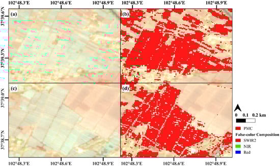
Figure 8.
The extraction results in large-scale farmlands. The main PMC can be extracted with the boundary between PMC also clearly. (a,c) the false-color composite (R = SWIR2, G = NIR, B = Red) images and (b,d) the extraction results (red part means PMC) above the false-color composite.
Considering the underlying surface in the SRB is not homogeneous, and the cropland is fragmentary, the PMC always mixes with other ground objects such as farmland without plastic, vegetation, or impervious surface. The TPEM were applied in the area with the complex mixed surfaces. Figure 9 was located where the town was surrounded by farmland already covered or not covered by plastic mulch. Although it is hard to distinguish the boundary between PMC and farmland without plastic, the TPEM can still extract PMC from a complex mixed surface.
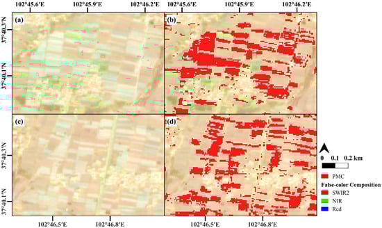
Figure 9.
The extraction results in a complex mixed surface, where the PMC is mixed with impervious surface, vegetation, and farmland not covered by plastic mulch. (a,c) the false-color composite (R = SWIR2, G = NIR, B = Red) images and (b,d) the extraction results (red part means PMC) above the false-color composite.
As mentioned in the spectral characteristic analysis, PMC shares a similar characteristic curve with sand, impervious surface, sand, and farmland. In the SRB, the PMC mixes with waterproof surfaces and farmland. Nevertheless, the sand, due to its high reflection similar to PMC and large area, is easy to be misidentified as PMC. Figure 10 shows an area located at the edge of the desert. The main PMC can be extracted, and there is little misidentification.
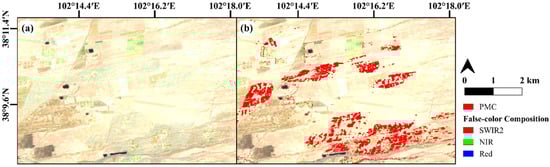
Figure 10.
The extraction results in the edge of the desert. As one of the most similar ground objects, the sand can be excluded from the PMC extraction results. (a) the false-color composite (R = SWIR2, G = NIR, B = Red) images and (b) the extraction results (red part means PMC) above the false-color composite.
3.3. Accuracy Assessment of PMC Extraction Rules
To evaluate the accuracy of the TPEM, all sample points were used to calculate the confusion matrix and related accuracy assessment indices. The confusion matrix is shown in Table 5. The OA can reach 0.9234 QD is only 0.0541, and AD is only 0.0224.
Table 5.
The confusion matrix of the TPEM using all sample points.
Focus on the specific ground objects, the water, snow and vegetation points were all classified as non-PMC as the spectral curves of these ground objects are different from PMC. Although the spectral curves of sand and farmland are similar to the PMC, only few points were misclassified as PMC. As Table 6 shows, 43 impervious surface sample points were classified as PMC. Because impervious surface and PMC share similar spectral curves.
Table 6.
Specific ground objects classification results. Few non-PMC sample points were extracted as PMC, except impervious surface points, who have similar spectral curves with PMC.
However, some PMC that was not extracted by the TPEM will lead to an underestimate of the area of PMC. The reason will be discussed later.
3.4. PMC Extraction Rules Threshold Sensitivity Analysis
The sensitivity analysis of the TPEM was carried out to assess the influence of the rules’ threshold on the TPEM’s results. By adjusting the threshold of one rule and fixing the thresholds of two remaining rules, the extraction rules get changed, and the corresponding extraction results are different. The OA, QD, and AD were calculated to evaluate the performance of different combinations of thresholds. As listed in Table 7, the change in the threshold of mPMCI will lead to a slight deterioration in performance. QD shows a downward trend, AD is increasing, and OA rises and then falls with the decreasing of mPMCI’s threshold.
Table 7.
The summary of overall accuracy, quantity disagreement, and allocation disagreement at different lower threshold values in the mPMCI band.
Considering the NDVI and SWIR2 bands have two thresholds of both upper and lower compared to the mPMCI only has one lower threshold, this paper set three ways of changing the thresholds of NDVI and SWIR2 bands, including (1) moving the threshold interval without changing the range of the threshold interval, (2) only adjust the upper threshold and (3) only adjust the lower threshold. As listed in Table 8, compared to adjusting the upper and lower threshold of NDVI, moving the threshold interval of NDVI without changing the range of the threshold interval has a more significant impact in the performance of the TPEM. The results of SWIR2 show the same pattern in Table 8 too. In the first way, with reducing the threshold interval of NDVI and SWIR2 band, QD fall then rise, and AD present downward trend. In the second way, with reducing the upper thresholds of NDVI and SWIR2 band, QD present upward trend and AD present opposite trend. In the third way, with reducing the lower thresholds of NDVI and SWIR2 band, QD present upward trend and AD present downward trend, which is opposite to the second way. In general, the three rules have good robustness, even in the worst situation, the OA can higher than 0.87, QD can lower than 0.11, and AD can lower than 0.12. A slight adjustment of the thresholds does not significantly affect the extraction results.
Table 8.
The summary of overall accuracy, quantity disagreement, and allocation disagreement at different combinations of lower and upper threshold values in the SWIR2 band and NDVI band.
3.5. Long-Term PMC Extraction Results
To understand the use of plastic mulch in the SRB over the past few years, the TPEM were applied in the SRB from 2011 to 2021. The ratio of PMC to total farmland in each year was calculated using FROM-GLC datasets as mentioned in Table 3. Considering the limited land cover data, the FROM-GLC 2015 dataset was applied from 2011 to 2015, and the FROM-GLC 2017 dataset was applied from 2016 to 2021. After filtering the cropland area, the TPEM was applied to the cropland to avoid the influence of other ground objects. Then, both cropland and PMC in each year were calculated to analyze the ratio of PMC to total farmland from 2011 to 2021. The ratio of PMC to total farmland is shown in Figure 11.
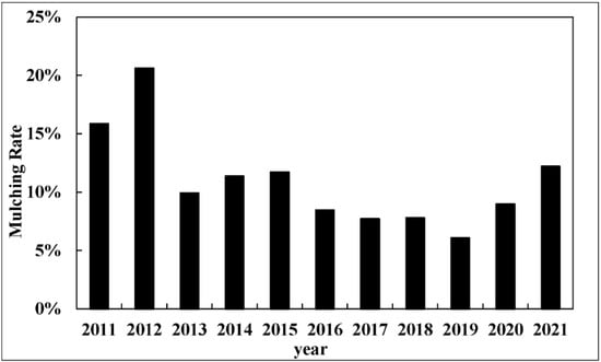
Figure 11.
The mulching rate change, which is the ratio of PMC area to total farmland area, in the SRB from 2011 to 2021.
The PMC extraction results images of 2011, 2014, 2017, and 2020 in the SRB are shown in Figure 12 to illustrate the spatial distribution of PMC. Farmland is distributed along the Shiyang River from upstream to downstream. In the upstream, which is also the southwest of the SRB, farmland accounts for more area than the northeast of the SRB. The distribution of PMC also shows a similar variation in that the southwest of the SRB has more PMC than the northwest of the SRB.
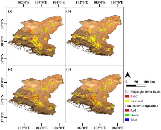
Figure 12.
The distribution of PMC in the SRB. (a–d) is extraction results from 2020, 2017, 2014, and 2011 laid on the true color composition map of SRB, respectively. The black line is the boundary of the SRB, the yellow part is filtered cropland using FROM-GLC datasets, and the red part is extracted PMC area.
4. Discussion
4.1. The Advantages of the Methods
Two PMC extraction methods, including the plastic-mulched farmland mapping algorithm (PFMA) proposed by Xiong et al. [17] and a decision-tree classifier proposed by Lu et al. [8], were selected to extract the PMC in the SRB, and the results of these three methods were compared. This was performed so that the effectiveness of the TPEM could be demonstrated. In Lu’s method [8], the same spectral characteristic was carried out. Five spectral features were used in the decision-tree classifier based on ENVI to generate classification rules which can classify all major ground objects, not only PMC. Remote sensing images of the SRB in 2020 were selected, and an isolated dataset including 1035 points of PMC and 1484 points of non-PMC was randomly selected and labeled by visual interpretation, as Section 2.2.2 mentioned. This dataset was used to evaluate and compare the extraction accuracy of the TPEM and other methods. Considering the PFMA used two time periods, the seeding period and growing period, two conditions, including the used and not used growing period, were tested to evaluate the effectiveness of PFMA under the conditions of the just-applied PMC.
In Table 9, the extraction results and accuracy assessment indices are calculated using the confusion matrix. The result shows that Lu’s decision-tree classifier does not apply to a more complex mixed surface, such as the SRB. Xiong’s PFMA can perform a high extraction accuracy, and the PFMA can obtain higher extraction accuracy using growing periods. At the same time, the TPEM can reach the same extraction accuracy as Xiong’s PFMA.
Table 9.
The PMC extracted results using Lu’s decision-tree classifier, Xiong’s PFMA, and TPEM proposed by this study. Xiong’ means using Xiong’s PFMA without using growing period data. The fractions represent the corrected classified sample points in this category/whole sample points in this category.
Figure 13 shows the extraction results in the SRB. Being influenced by the large area of sand and snow-covered Qilian Mountain, Lu’s decision-tree classifier cannot distinguish between these ground objects with PMC.
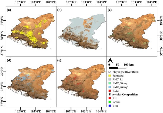
Figure 13.
The PMC extraction results using Lu’s decision-tree classifier, Xiong’s PFMA, and TPEM proposed by this study. The black line is the boundary of the SRB. (a) is the filtered farmland using FROM-GLC datasets, (b) is the PMC extracted by Lu’s decision-tree classifier, namely PMC_Lu, (c) is the PMC extracted by Xiong’s PFMA using the growing period data, namely PMC_Xiong, (d) is the PMC extracted by Xiong’s PFMA without using growing period data, namely PMC_Xiong’ (e) is the PMC extracted by this study, namely PMC.
Xiong’s PFMA can obtain a precise extraction result as the distribution of extracted PMC is consistent with that of farmland. However, under the conditions of not using growing period data, the misidentification of sand will cause the overestimation of PMC. Considering other ground objects except vegetation and PMC cannot reach a high NDVI value in the growing period, it is expected that some misidentification will occur without using growing period data.
Although there is misidentification, the TPEM performs well as the distribution of extracted PMC is consistent with that of farmland. This method can extract the PMC under the condition of the PMC has just been applied and have an ideal performance with only using a short period of data.
4.2. Error Analysis from the Point of Spectral
The spectral values of all ground objects were collected and analyzed to figure out why some sample points cannot be extracted as PMC. Figure 14 shows the differences in mPMCI, NDVI, and SWIR1 band among PMC, vegetation, impervious surface, sand, farmland, snow, and water in the SRB based on the sample points. It is clear that in the mPMCI band, PMC is significantly higher than other ground objects except for water. In the NDVI band, vegetation is higher than others, and water is lower than them. In the SWIR2 band, water and snow are lower than in others. However, the PMC, impervious surface, sand, and farmland were similar in the NDVI and SWIR2 bands. The mPMCI band plays a crucial role in distinguishing PMC with impervious surfaces, sand, and farmland. As in Figure 14a, the value of these three ground objects was out of the box of the PMC but within the error bar of the PMC, which means almost one-quarter of PMC share a similar spectral characteristic with these ground objects, and that is why in Table 5 the TPEM did not extract about a quarter PMC. Especially the impervious surface, its upper quantile is almost equal to the lower quantile of the PMC. It explained why there are still 43 impervious surface points were classified as PMC in Table 6. Although mPMCI can distinguish between these ground objects, there are still some sample points whose values are relatively low and will be classified as non-PMC.
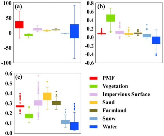
Figure 14.
Box plot of spectral features in different ground objects, including PMC, Vegetation, Impervious Surface, Sand, Farmland, Snow, and Water. (a) is the box plot of mPMCI, (b) is the box plot of NDVI, and (c) is the box plot of SWIR2.
5. Conclusions
The TPEM proposed by this paper was used to extract the PMC in the SRB between 1 April and 20 April 2020. This method modified an index to amplify the difference between PMC and ground objects with the same spectral characteristics. This method obtained 0.9234 overall accuracy when applied over complex mixed underlying surfaces and reduced the requirements of remote sensing data. Three main conditions, including large-scale farmland, PMC mixing with the complex mixed surfaces, and PMC near the desert, were considered for testing this method’s performance. The results showed that the user accuracy of PMC and non-PMC are 0.9371 and 0.9094, which means high precision of classification results. Only 0.0541 of QD and 0.0224 of AD revealed the TPEM can complete the correct classification of pixels. A slight adjustment of the thresholds does not significantly affect the extraction results. Even in the worst situation, the OA can higher than 0.87, QD can lower than 0.11, and AD can lower than 0.12. Then TPEM was used to extract the PMC in the SRB from 2011 to 2021 to monitor local PMF area change over decade. The extraction area was underestimated because about a quarter of the PMC and other ground objects show similar values in the mPMCI index.
The TPEM was compared with other methods to test its effectiveness. The comparison results show that TPEM can provide up to 0.9555 of OA only using remote sensing data during the seeding period. However, in the case that timeliness is not critical, TPEM may not obtain the highest extraction results. Limited by the short time window of PMC extraction, it is necessary to obtain high spatial and temporal resolution. The former can provide more precise ground truth and latter can provide more information during the time window, avoiding the absence of images within the time window. Furthermore, we did not test the performance of TPEM in other regions yet. Therefore, other ground objects not considered may influence the effectiveness of TPEM. In future work, we would like to analyze the regional climate response to plastic mulch.
Author Contributions
Conceptualization, S.Q., C.F. and L.C. (Lei Cheng); methodology, C.F., S.Q. and L.C. (Lei Cheng); software, C.F., K.Z. and L.C. (Liwei Chang); data curation, C.F., K.Z. and L.C. (Liwei Chang); writing-original draft C.F., S.Q., A.T. and L.C. (Lei Cheng); writing-review and editing, C.F., S.Q., A.T., L.C. (Lei Cheng) and P.L.; supervision, S.Q., L.C. (Lei Cheng) and P.L.; funding acquisition, S.Q. All authors have read and agreed to the published version of the manuscript.
Funding
This research was funded by Postdoctoral Research Foundation of China (grant No. 2020M682477) and the Fundamental Research Funds for the Central Universities (grant No. 2042021kf0053).
Data Availability Statement
Publicly available datasets were used in this study. These data can be found in: https://sentinel.esa.int/web/sentinel/user-guides/sentinel-2-msi/product-types/level-2a (accessed on: 8 December 2021), https://www.usgs.gov/landsat-missions/landsat-surface-reflectance (accessed on 8 December 2021), https://lpdaac.usgs.gov/products/mod09a1v006/ (accessed on 8 December 2021), and http://data.ess.tsinghua.edu.cn/ (accessed on 17 August 2021).
Acknowledgments
We would like to thank the fundings and all data providers mentioned above. We sincerely thank the anonymous reviewers and editors of the journal for providing helpful comments to improve the manuscript.
Conflicts of Interest
The authors declare no conflict of interest.
References
- Liu, C.A.; Jin, S.L.; Zhou, L.M.; Jia, Y.; Li, F.M.; Xiong, Y.C.; Li, X.G. Effects of plastic film mulch and tillage on maize productivity and soil parameters. Eur. J. Agron. 2009, 31, 241–249. [Google Scholar] [CrossRef]
- Li, S.; Kang, S.; Li, F.; Zhang, L. Evapotranspiration and crop coefficient of spring maize with plastic mulch using eddy covariance in northwest China. Agric. Water Manag. 2008, 95, 1214–1222. [Google Scholar] [CrossRef]
- Bu, L.; Liu, J.; Zhu, L.; Luo, S.; Chen, X.; Li, S.; Lee Hill, R.; Zhao, Y. The effects of mulching on maize growth, yield and water use in a semi-arid region. Agric. Water Manag. 2013, 123, 71–78. [Google Scholar] [CrossRef]
- Yang, Q.; Zuo, H.; Xiao, X.; Wang, S.; Chen, B.; Chen, J. Modelling the effects of plastic mulch on water, heat and CO2 fluxes over cropland in an arid region. J. Hydrol. 2012, 452–453, 102–118. [Google Scholar] [CrossRef]
- Kasirajan, S.; Ngouajio, M. Polyethylene and biodegradable mulches for agricultural applications: A review. Agron. Sustain. Dev. 2012, 32, 501–529. [Google Scholar] [CrossRef]
- Liu, E.K.; He, W.Q.; Yan, C.R. ‘White revolution’ to ‘white pollution’-agricultural plastic film mulch in China. Environ. Res. Lett. 2014, 9, 91001. [Google Scholar] [CrossRef]
- Gao, H.; Yan, C.; Liu, Q.; Ding, W.; Chen, B.; Li, Z. Effects of plastic mulching and plastic residue on agricultural production: A meta-analysis. Sci. Total Environ. 2019, 651, 484–492. [Google Scholar] [CrossRef]
- Lu, L.; Di, L.; Ye, Y. A Decision-Tree Classifier for Extracting Transparent Plastic-Mulched Landcover from Landsat-5 TM Images. IEEE J. Sel. Top. Appl. Earth Obs. Remote Sens. 2014, 7, 4548–4558. [Google Scholar] [CrossRef]
- Tariq, A.; Yan, J.; Gagnon, A.S.; Riaz Khan, M.; Mumtaz, F. Mapping of cropland, cropping patterns and crop types by combining optical remote sensing images with decision tree classifier and random forest. Geo-Spat. Inf. Sci. 2022. [Google Scholar] [CrossRef]
- Lu, L.; Tao, Y.; Di, L. Object-Based Plastic-Mulched Landcover Extraction Using Integrated Sentinel-1 and Sentinel-2 Data. Remote Sens. 2018, 10, 1820. [Google Scholar] [CrossRef]
- Hasituya; Chen, Z. Mapping Plastic-Mulched Farmland with Multi-Temporal Landsat-8 Data. Remote Sens. 2017, 9, 557. [Google Scholar] [CrossRef]
- Breiman, L.; Friedman, J.H.; Olshen, R.A.; Stone, C.J. Classification and Regression Trees; Routledge: London, UK, 1984. [Google Scholar]
- Wahla, S.S.; Kazmi, J.H.; Sharifi, A.; Shirazi, S.A.; Tariq, A.; Joyell Smith, H. Assessing spatio-temporal mapping and monitoring of climatic variability using SPEI and RF machine learning models. Geocarto Int. 2022, 38, 21. [Google Scholar] [CrossRef]
- Gislason, P.O.; Benediktsson, J.A.; Sveinsson, J.R. Random Forests for land cover classification. Pattern Recogn. Lett. 2006, 27, 294–300. [Google Scholar] [CrossRef]
- Cortes, C.; Vapnik, V. Support-vector networks. Mach. Learn. 1995, 20, 273–297. [Google Scholar] [CrossRef]
- Hao, P.; Chen, Z.; Tang, H.; Li, D.; Li, H. New Workflow of Plastic-Mulched Farmland Mapping using Multi-Temporal Sentinel-2 data. Remote Sens. 2019, 11, 1353. [Google Scholar] [CrossRef]
- Xiong, Y.; Zhang, Q.; Chen, X.; Bao, A.; Zhang, J.; Wang, Y. Large Scale Agricultural Plastic Mulch Detecting and Moni-toring with Multi-Source Remote Sensing Data: A Case Study in Xinjiang, China. Remote Sens. 2019, 11, 2088. [Google Scholar] [CrossRef]
- Tariq, A.; Mumtaz, F.; Zeng, X.; Baloch, M.Y.J.; Moazzam, M.F.U. Spatio-temporal variation of seasonal heat islands mapping of Pakistan during 2000–2019, using day-time and night-time land surface temperatures MODIS and meteorological stations data. Remote Sens. Appl. Soc. Environ. 2022, 27, 100779. [Google Scholar] [CrossRef]
- Zhang, C.; Wang, X.; Li, J.; Hua, T. Roles of climate changes and human interventions in land degradation: A case study by net primary productivity analysis in China’s Shiyanghe Basin. Environ. Earth Sci. 2011, 64, 2183–2193. [Google Scholar] [CrossRef]
- Qin, S.; Li, S.; Kang, S.; Du, T.; Tong, L.; Ding, R. Can the drip irrigation under film mulch reduce crop evapotranspiration and save water under the sufficient irrigation condition? Agric. Water Manag. 2016, 177, 128–137. [Google Scholar] [CrossRef]
- Li, F.M.; Wang, J.; Xu, J.Z.; Xu, H.L. Productivity and soil response to plastic film mulching durations for spring wheat on entisols in the semiarid Loess Plateau of China. Soil Till. Res. 2004, 78, 9–20. [Google Scholar] [CrossRef]
- Zhang, Y.; Wang, F.; Shock, C.C.; Yang, K.; Kang, S.; Qin, J.; Li, S. Influence of different plastic film mulches and wetted soil percentages on potato grown under drip irrigation. Agric. Water Manag. 2017, 180, 160–171. [Google Scholar] [CrossRef]
- Yang, Q.; Liu, M.; Zhang, Z.; Yang, S.; Ning, J.; Han, W. Mapping Plastic Mulched Farmland for High Resolution Images of Unmanned Aerial Vehicle Using Deep Semantic Segmentation. Remote Sens. 2019, 11, 2008. [Google Scholar] [CrossRef]
- Yang, D.; Chen, J.; Zhou, Y.; Chen, X.; Chen, X.; Cao, X. Mapping plastic greenhouse with medium spatial resolution satellite data: Development of a new spectral index. ISPRS J. Photogramm. 2017, 128, 47–60. [Google Scholar] [CrossRef]
- Hu, Z.-Q.; Tian, X.-H.; Zhang, J.-D.; Bao, X.-G.; Ma, Z.-M. Research on amount and low of water requirement in Shiyang River Basin. Agric. Res. Arid Areas 2011, 29, 1–6. [Google Scholar]
- Third National Agricultural Census Leading Group Office. Compilation of the Third National Agricultural Census in Gansu Province; China Statistics Press: Beijing, China, 2020.
- Gong, P.; Wang, J.; Yu, L.; Zhao, Y.; Zhao, Y.; Liang, L.; Niu, Z.; Huang, X.; Fu, H.; Liu, S.; et al. Finer resolution observation and monitoring of global land cover: First mapping results with Landsat TM and ETM+ data. Int. J. Remote Sens. 2012, 34, 2607–2654. [Google Scholar] [CrossRef]
- Gong, P.; Liu, H.; Zhang, M.; Li, C.; Wang, J.; Huang, H.; Clinton, N.; Ji, L.; Li, W.; Bai, Y.; et al. Stable classification with limited sample: Transferring a 30-m resolution sample set collected in 2015 to mapping 10-m resolution global land cover in 2017. Sci. Bull. 2019, 64, 370–373. [Google Scholar] [CrossRef]
- Liu, H.; Gong, P.; Wang, J.; Clinton, N.; Bai, Y.; Liang, S. Annual dynamics of global land cover and its long-term changes from 1982 to 2015. Earth Syst. Sci. Data 2020, 12, 1217–1243. [Google Scholar] [CrossRef]
- Google. Sentinel-2 MSI: MultiSpectral Instrument, Level-2A. Available online: https://developers.google.cn/earth-engine/datasets/catalog/COPERNICUS_S2_SR (accessed on 12 August 2022).
- Google. USGS Landsat 8 Level 2, Collection 2, Tier 1. Available online: https://developers.google.cn/earth-engine/datasets/catalog/LANDSAT_LC08_C02_T1_L2 (accessed on 12 August 2022).
- Google. USGS Landsat 7 Level 2, Collection 2, Tier 1. Available online: https://developers.google.cn/earth-engine/datasets/catalog/LANDSAT_LE07_C02_T1_L2 (accessed on 12 August 2022).
- Google. MOD09A1.006 Terra Surface Reflectance 8-Day Global 500 m. Available online: https://developers.google.cn/earth-engine/datasets/catalog/MODIS_006_MOD09A1 (accessed on 12 August 2022).
- Aguilar, M.Á.; Jiménez-Lao, R.; Nemmaoui, A.; Aguilar, F.J.; Koc-San, D.; Tarantino, E.; Chourak, M. Evaluation of the Consistency of Simultaneously Acquired Sentinel-2 and Landsat 8 Imagery on Plastic Covered Greenhouses. Remote Sens. 2020, 12, 2015. [Google Scholar] [CrossRef]
- D’Odorico, P.; Gonsamo, A.; Dammm, A.; Schaepman, M.E. Experimental Evaluation of Sentinel-2 Spectral Response Functions for NDVI Time-Series Continuity. IEEE Trans. Geosci. Remote 2013, 51, 1336–1348. [Google Scholar] [CrossRef]
- Mandanici, E.; Bitelli, G. Preliminary Comparison of Sentinel-2 and Landsat 8 Imagery for a Combined Use. Remote Sens 2016, 8, 1014. [Google Scholar] [CrossRef]
- Roy, D.P.; Kovalskyy, V.; Zhang, H.K.; Vermote, E.F.; Yan, L.; Kumar, S.S.; Egorov, A. Characterization of Landsat-7 to Landsat-8 reflective wavelength and normalized difference vegetation index continuity. Remote Sens. Environ. 2016, 185, 57–70. [Google Scholar] [CrossRef] [PubMed]
- Foody, G.M. Status of land cover classification accuracy assessment. Remote Sens. Environ. 2002, 80, 185–201. [Google Scholar] [CrossRef]
- Pontius, R.G., Jr.; Millones, M. Death to Kappa: Birth of quantity disagreement and allocation disagreement for accuracy assessment. Int. J. Remote Sens. 2011, 32, 4407–4429. [Google Scholar] [CrossRef]
- Congalton, R.G. A review of assessing the accuracy of classifications of remotely sensed data. Remote Sens. Environ. 1991, 37, 35–46. [Google Scholar] [CrossRef]
- De’Ath, G.; Fabricius, K.E. Classification and regression trees: A powerful yet simple technique for ecological data analysis. Ecology 2000, 81, 3178–3192. [Google Scholar] [CrossRef]
Publisher’s Note: MDPI stays neutral with regard to jurisdictional claims in published maps and institutional affiliations. |
© 2022 by the authors. Licensee MDPI, Basel, Switzerland. This article is an open access article distributed under the terms and conditions of the Creative Commons Attribution (CC BY) license (https://creativecommons.org/licenses/by/4.0/).