
Identifying Coffee Agroforestry System Types Using Multitemporal Sentinel-2 Data and Auxiliary Information

 , ,
, ,  and
and 
Abstract
:1. Introduction
2. Materials and Methods
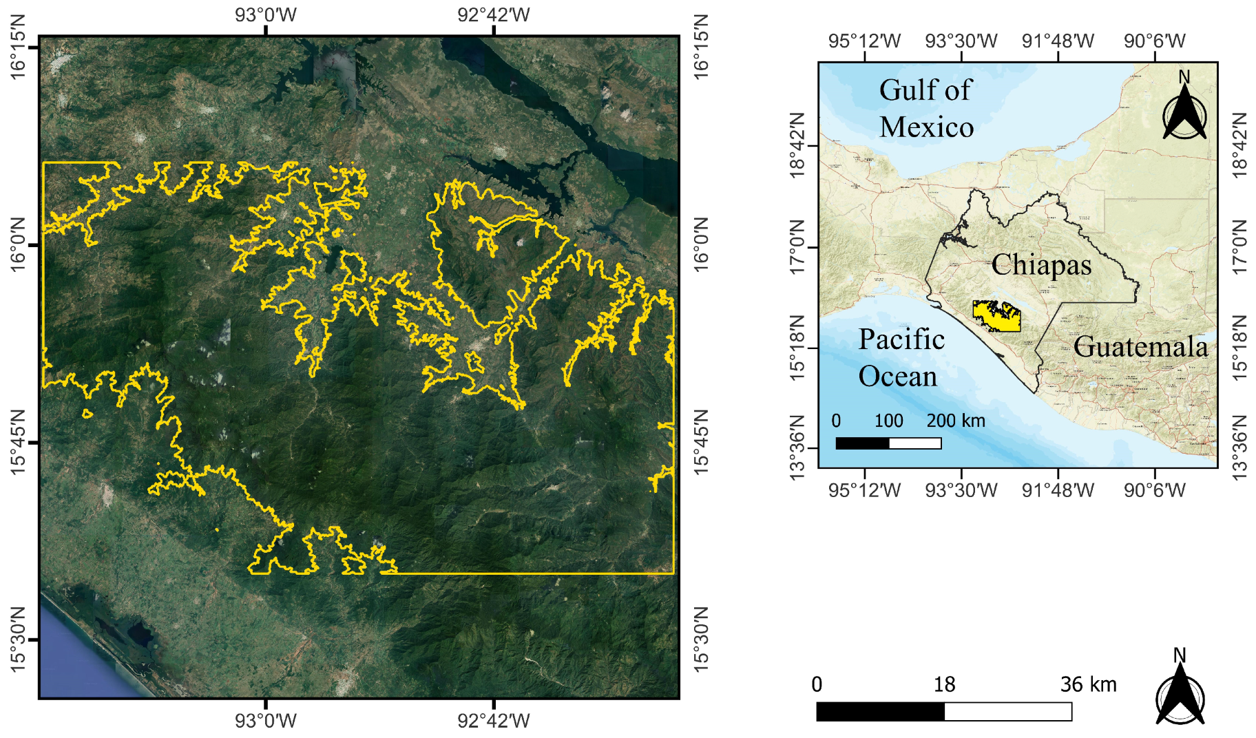
2.1. Study Area
2.2. Field Data and Characterization of Agroforestry Systems
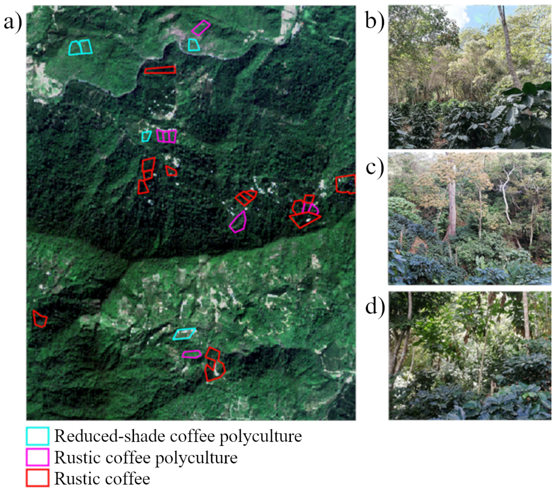
- Reduced-shade coffee polyculture. This system has one or two tree strata and an understory layer with coffee plants. The highest stratum shows some trees of natural vegetation, usually the tallest trees (>7 m). When there is an intermediate stratum, it usually includes fruit and timber tree species; the most common species are naranja (Citrus × sinensis (L.) Osb.), aguacate (Persea americana Mill.), plátano (Musa paradisiaca L.), zapote (Pouteria sapota (Jacq.) H.E. Moore and Stearn), and mango (Mangifera indica L.). The percent shade is generally less than or equal to 30%, the tree density varies from 16 to 30 trees per hectare, and the density of coffee plants ranges from 2500 to 4400 plants per hectare. Although trees are not evenly distributed, the distance between shade trees is usually wide, so there are open areas, and coffee plants are frequently apparent in high-resolution images (Figure 2b).
- Rustic coffee polyculture. This AFS has two tree strata and an understory of coffee plants. The highest stratum includes trees of natural vegetation, in some cases alternating with introduced timber trees, mainly cedro (Cedrela odorata L.) and roble (Quercus robur L.); the average height of this stratum is 10 m. The second stratum generally comprises introduced species with a mean height of 6 m, commonly chalum (Inga vera Willd.), caspirol (Inga laurina (Sw.) Willd.), paterna (Inga spuria H and B. Ex Willd.), and fruit trees such as naranja (Citrus × sinensis (L.) Osb.), among others. The percent shade ranges from 30% to 60%. The density of shade trees varies between 24 and 38 trees/ha, and the density of coffee plants, between 2500 and 4800 plants/ha. In satellite images, these systems appear more homogeneous in color compared to forests and tropical forests and are less fragmented (Figure 2c) and less intensely colored than reduced-shade polycultures.
- Rustic coffee. This system also has one or two strata of tree vegetation; the highest stratum is dominated by species of natural vegetation, with occasional introduced trees. The intermediate stratum consists mainly of timber trees, including chalum (Inga vera Willd.), caspirol (Inga laurina (Sw.) Willd.) and paterna (Inga spuria H and B. Ex Willd.) of lower height.The percent shade is greater than 60%. Compared to the other AFS classes, this class has a higher density of shade trees (30–44 trees/ha), with a similar density of coffee plants (2500–3300 plants/ha). This system is the one leading to greater spectral confusion with forests and tropical forests because the three show similar tonalities and texture patterns (Figure 2d).
2.3. Imagery and Auxiliary Data
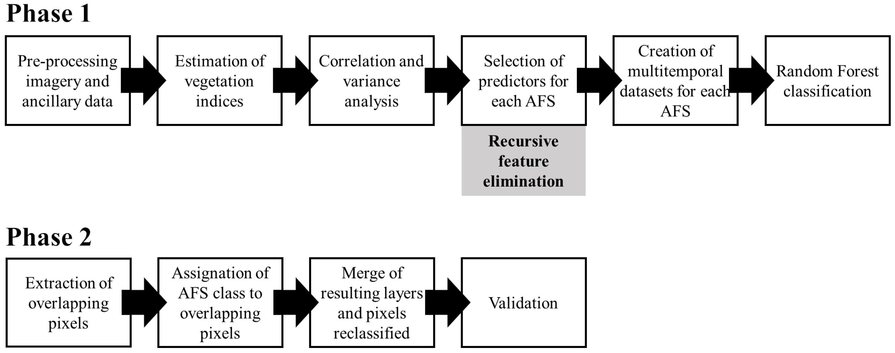
2.4. Image Processing
2.5. Data Analysis and Land Cover Classification
2.6. Map Validation
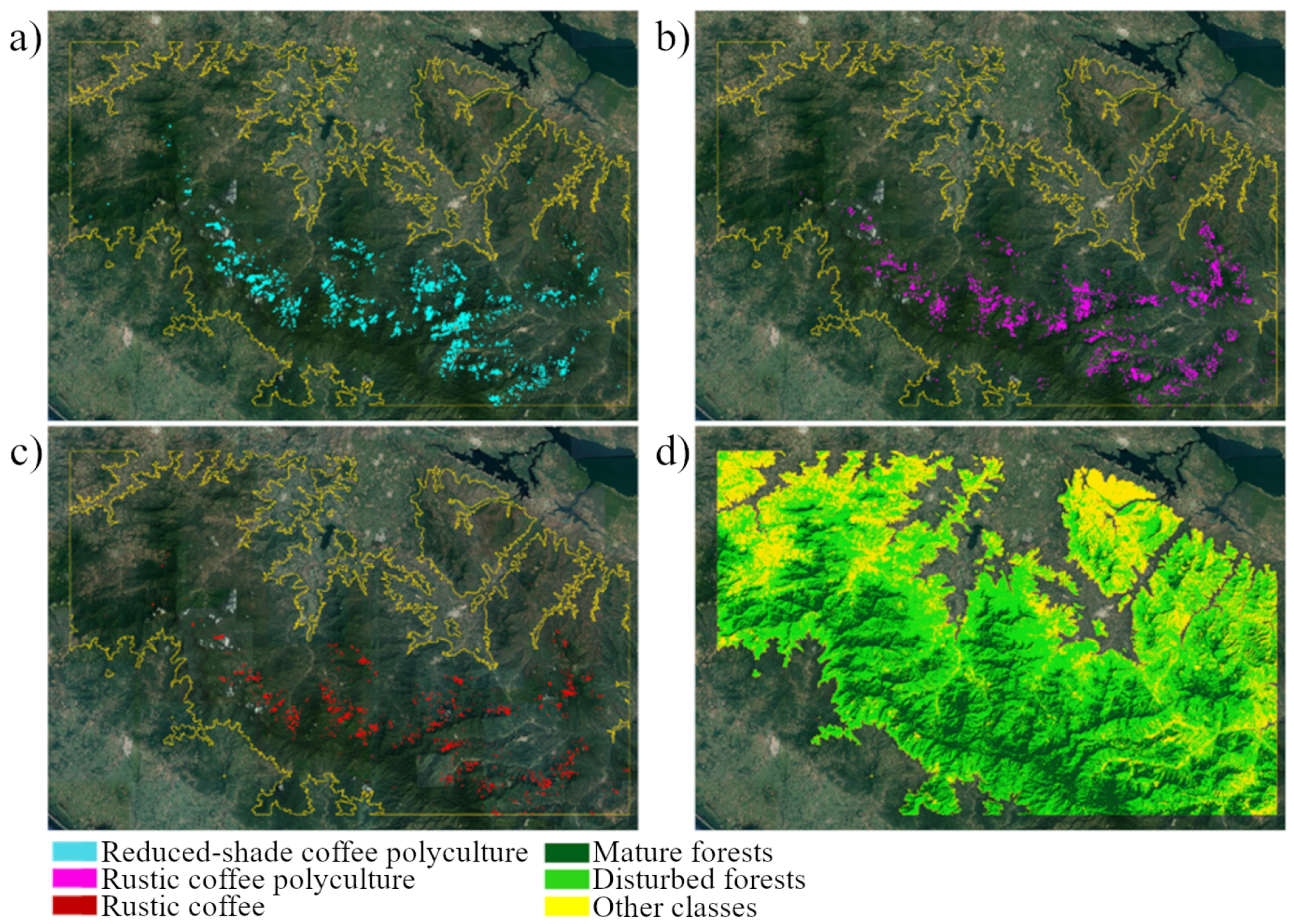
3. Results
3.1. Selecting Predictors and Applying the Classification Model
3.2. Model Validation
4. Discussion
5. Conclusions
Author Contributions
Funding
Data Availability Statement
Acknowledgments
Conflicts of Interest
References
- ITC. The Coffee Guide; Technical Report; The International Trade Centre (ITC): Geneva, Switzerland, 2021. [Google Scholar]
- Perfecto, I.; Jiménez-Soto, M.E.; Vandermeer, J. Coffee Landscapes Shaping the Anthropocene. Curr. Anthropol. 2019, 60, S236–S250. [Google Scholar] [CrossRef]
- Harvey, C.A.; Martínez-Rodríguez, M.R.; Cárdenas’, J.M.; Avelino, J.; Rapidel, B.; Vignola, R.; Donatti, C.I.; Vilchez-Mendoza, S. The Use of Ecosystem-based Adaptation Practices by Smallholder Farmers in Central America. Agric. Ecosyst. Environ. 2017, 246, 279–290. [Google Scholar] [CrossRef]
- CEDRSSA. Reporte del café en México: Diagnóstico y perspectiva; Technical Reports; Cámara de Diputados: Ciudad de México, Mexico, 2018. [Google Scholar]
- Farfán-Valencia, F. Descripción de la Estructura del Dosel Arbóreo al Interior de un Sistema Agroforestal con Café; Technical Report; Centro Nacional de Investigaciones de Café, Manizales: Caldas, Colombia, 2019. [Google Scholar]
- Jose, S. Environmental Impacts and Benefits of Agroforestry. In Oxford Research Encyclopedia of Environmental Science; Oxford University Press: Oxford, UK, 2019. [Google Scholar] [CrossRef]
- Ospina, C. Climate and Economic Benefits of Agroforestry Systems; Climate Institute: Washington, DC, USA, 2017; p. 11. [Google Scholar]
- DaMatta, F.; Nelson, R. Sustainable Production of Coffee In Agroforestry Systems in the Neotropics: An Agronomic and Ecophysiological Approach. Agron. Colomb. 2007, 1, 113–123. [Google Scholar]
- Montagnini, F.; Somarriba, E.; Murgueitio, E.; Fassola, H.; Eibl, B. Función de los sistemas agroforestales en la adaptación y mitigación del cambio climático. In Sistemas Agroforestales. Funciones Productivas, Socioeconómicas y Ambientales; CATIE: Turrialba, Costa Rica, 2015; pp. 269–298. [Google Scholar]
- Harvey, C.A.; Pritts, A.A.; Zwetsloot, M.J.; Jansen, K.; Pulleman, M.M.; Armbrecht, I.; Avelino, J.; Barrera, J.F.; Bunn, C.; García, J.H.; et al. Transformation of Coffee-growing Landscapes Across Latin America. A Review. Agron. Sustain. Dev. 2021, 41, 62. [Google Scholar] [CrossRef]
- Toledo, V.M.; Moguel, P. Coffee and Sustainability: The Multiple Values of Traditional Shaded Coffee. J. Sustain. Agric. 2012, 36, 353–377. [Google Scholar] [CrossRef]
- Jha, S.; Bacon, C.M.; Philpott, S.M.; Rice, R.A.; Méndez, V.E.; Läderach, P. A Review of Ecosystem Services, Farmer Livelihoods, and Value Chains in Shade Coffee Agroecosystems; Spinger: Berlin, Germany, 2011; pp. 141–208. [Google Scholar] [CrossRef]
- INCAFECH. Datos importantes del café.
- Valencia, V.; García-Barrios, L.; Sterling, E.J.; West, P.; Meza-Jiménez, A.; Naeem, S. Smallholder response to environmental change: Impacts of coffee leaf rust in a forest frontier in Mexico. Land Use Policy 2018, 79, 463–474. [Google Scholar] [CrossRef]
- Higuera-Ciapara, I.; Rivera-Ramírez, J. Chiapas: Problemáticas del Sector Cafetalero; Centro de Investigación y Asistencia en Tecnología y Diseño del Estado de Jalisco: Guadalajara, Mexico, 2018. [Google Scholar]
- Boell, M.; Ramos Alves, H.; Volpato, M.; Ferreira, D.; Lacerda, W. Exploiting Feature Extraction Techniques for Remote Sensing Image Classification. IEEE Lat. Am. Trans. 2018, 16, 2657–2664. [Google Scholar] [CrossRef]
- Hunt, D.A.; Tabor, K.; Hewson, J.H.; Wood, M.A.; Reymondin, L.; Koenig, K.; Schmitt-Harsh, M.; Follett, F. Review of Remote Sensing Methods to Map Coffee Production Systems. Remote Sens. 2020, 12, 2041. [Google Scholar] [CrossRef]
- Souza, C.G.; Carvalho, L.; Aguiar, P.; Arantes, T.B. Algoritmos de Aprendizagem de Máquina e Variáveis de Sensoramento Remoto para o Mapamento da Cafeicultura. Bol. De Ciências Geodésicas 2016, 22, 751–773. [Google Scholar] [CrossRef]
- Schmitt-Harsh, M.; Sweeney, S.P.; Evans, T.P. Classification of Coffee-Forest Landscapes Using Landsat TM Imagery and Spectral Mixture Analysis. Photogramm. Eng. Remote Sens. 2013, 79, 457–468. [Google Scholar] [CrossRef]
- Mosomtai, G.; Odindi, J.; Abdel-Rahman, E.M.; Babin, R.; Fabrice, P.; Mutanga, O.; Tonnang, H.E.Z.; David, G.; Landmann, T. Landscape Fragmentation in Coffee Agroecological Subzones in Central Kenya: A Multiscale Remote Sensing Approach. J. Appl. Remote Sens. 2020, 14, 044513. [Google Scholar] [CrossRef]
- Hebbar, R.; Ravishankar, H.M.; Trivedi, S.; Manjula, V.B.; Kumar, N.M.; Mukharib, D.S.; Mote, J.K.; Sudeesh, S.; Raj, U.; Raghuramulu, Y.; et al. National Level Inventory of Coffee Plantations Using High Resolution Satellite Data. Int. Arch. Photogramm. Remote Sens. Spat. Inf. Sci. 2019, XLII-3/W6, 293–298. [Google Scholar] [CrossRef]
- Bautista Calderon, E.A.; Ordaz Chaparro, V.M.; Gutiérrez Castorena, M.d.C.; Gutiérrez Castorena, E.V.; Cajuste Bontemps, L. Sistemas agroforestales de café en Veracruz, México: Identificación y cuantificación espacial usando SIG, percepción remota y conocimiento local. Rev. Terra Latinoam. 2018, 36. [Google Scholar] [CrossRef]
- Kelley, L.C.; Pitcher, L.; Bacon, C. Using Google Earth Engine to Map Complex Shade-Grown Coffee Landscapes in Northern Nicaragua. Remote Sens. 2018, 10, 952. [Google Scholar] [CrossRef]
- Tridawati, A.; Wikantika, K.; Susantoro, T.M.; Harto, A.B.; Darmawan, S.; Yayusman, L.F.; Ghazali, M.F. Mapping the Distribution of Coffee Plantations from Multi-Resolution, Multi-Temporal, and Multi-Sensor Data Using a Random Forest Algorithm. Remote Sens. 2020, 12, 3933. [Google Scholar] [CrossRef]
- Ortega-Huerta, M.A.; Komar, O.; Price, K.P.; Ventura, H.J. Mapping coffee plantations with Landsat imagery: An example from El Salvador. Int. J. Remote Sens. 2012, 33, 220–242. [Google Scholar] [CrossRef]
- Chemura, A.; Mutanga, O.; Odindi, J. Modelling Leaf Chlorophyll Content in Coffee (Coffea Arabica) Plantations Using Sentinel 2 Msi Data. In Proceedings of the IGARSS IEEE International Geoscience and Remote Sensing Symposium, Valencia, Spain, 22–27 July 2018; pp. 8228–8231. [Google Scholar] [CrossRef]
- Figueroa-Hernández, E.; Pérez-Soto, F.; Godínez-Montoya, L. La produccion y el consumo del café. ECORFAN 2015, 1, 64–82. [Google Scholar]
- INEGI. Continuo de Elevaciones de México (CEM 3.0). 2019. Available online: https://www.inegi.org.mx/app/geo2/elevacionesmex/ (accessed on 7 January 2019).
- SMN. Resúmenes Mensuales de Temperaturas y Lluvia; SMN: Mexico City, Mexico, 2019. [Google Scholar]
- González-Espinosa, M.; Ramírez-Marcial, N.; Gómez-Pineda, E.; Parra-Vázquez, M.R.; Díaz-Hernández, B.M.; Musálem-Castillejos, K. Vulnerabilidad Ambiental y Social. Perspectivas de Restauración de Bosques en las Partes Altas de la Sierra Madre de Chiapas. Investig. Ambient. Cienc. Y Política Pública 2015, 6, 90–91. [Google Scholar]
- Moguel, P.; Toledo, V. Biodiversity Conservation in Traditional Coffee Systems of Mexico. Conserv. Biol. 1999, 13, 11–21. [Google Scholar] [CrossRef]
- Hernández-Stefanoni, J.L.; Castillo-Santiago, M.A.; Mas, J.F.; Wheeler, C.E.; Andres-Mauricio, J.; Tun-Dzul, F.; George-Chacón, S.P.; Reyes-Palomeque, G.; Castellanos-Basto, B.; Vaca, R.; et al. Improving aboveground biomass maps of tropical dry forests by integrating LiDAR, ALOS PALSAR, climate and field data. Carbon Balance Manag. 2020, 15, 15. [Google Scholar] [CrossRef] [PubMed]
- Brodu, N. Super-Resolving Multiresolution Images With Band-Independent Geometry of Multispectral Pixels. IEEE Trans. Geosci. Remote Sens. 2017, 55, 4610–4617. [Google Scholar] [CrossRef]
- Wu, C.; Niu, Z.; Tang, Q.; Huang, W. Estimating chlorophyll content from hyperspectral vegetation indices: Modeling and validation. Agric. For. Meteorol. 2008, 148, 1230–1241. [Google Scholar] [CrossRef]
- Haboudane, D.; Miller, J.R.; Tremblay, N.; Zarco-Tejada, P.J.; Dextraze, L. Integrated Narrow-band Vegetation Indices for Prediction of Crop Chlorophyll Content for Application to Precision Agriculture. Remote Sens. Environ. 2002, 81, 416–426. [Google Scholar] [CrossRef]
- Filipponi, F. Sentinel-1 GRD Preprocessing Workflow. Proceedings 2019, 18, 11. [Google Scholar] [CrossRef]
- Hunt, E.R.; Daughtry, C.; Eitel, J.U.H.; Long, D.S. Remote Sensing Leaf Chlorophyll Content Using a Visible Band Index. Agron. J. 2011, 103, 1090–1099. [Google Scholar] [CrossRef]
- Main, R.; Cho, M.A.; Mathieu, R.; O’Kennedy, M.M.; Ramoelo, A.; Koch, S. An Investigation Into Iobust Spectral Indices for Leaf Chlorophyll Estimation. ISPRS J. Photogramm. Remote Sens. 2011, 66, 751–761. [Google Scholar] [CrossRef]
- Escadafal, R.; Belghith, A.; Ben-Moussa, H. Indices Spectraux Pour la Dégradation des Milieux Naturels en Tunisie Aride. In Proceedings of the 6eme Symposium International Sur les Mesures Physiques et Signatures en Télédétection, Val d’Isère, France, 17–24 January 1994; pp. 253–259. [Google Scholar]
- Bannari, A.; Morin, D.; Bonn, F.; Huete, A.R. A Review of Vegetation Indices. Remote Sens. Rev. 1995, 13, 95–120. [Google Scholar] [CrossRef]
- Darst, B.F.; Malecki, K.C.; Engelman, C.D. Using recursive feature elimination in random forest to account for correlated variables in high dimensional data. BMC Genet. 2018, 19, 65. [Google Scholar] [CrossRef]
- Breiman, L. Random forests. Mach. Learn. 2001, 45, 5–32. [Google Scholar] [CrossRef]
- Olofsson, P.; Foody, G.M.; Herold, M.; Stehman, S.V.; Woodcock, C.E.; Wulder, M.A. Good practices for estimating area and assessing accuracy of land change. Remote Sens. Environ. 2014, 148, 42–57. [Google Scholar] [CrossRef]
- Olofsson, P.; Foody, G.M.; Stehman, S.V.; Woodcock, C.E. Making better use of accuracy data in land change studies: Estimating accuracy and area and quantifying uncertainty using stratified estimation. Remote Sens. Environ. 2013, 129, 122–131. [Google Scholar] [CrossRef]
- Esri. World Imagery. Available online: https://www.arcgis.com/home/item.html?id=10df2279f9684e4a9f6a7f08febac2a9 (accessed on 15 January 2019).
- Cordero-Sancho, S.; Sader, S.A. Spectral analysis and classification accuracy of coffee crops using Landsat and a topographic-environmental model. Int. J. Remote Sens. 2007, 28, 1577–1593. [Google Scholar] [CrossRef]
- Maskell, G.; Chemura, A.; Nguyen, H.; Gornott, C.; Mondal, P. Integration of Sentinel optical and radar data for mapping smallholder coffee production systems in Vietnam. Remote Sens. Environ. 2021, 266, 112709. [Google Scholar] [CrossRef]
- Gomez, C.; Mangeas, M.; Petit, M.; Corbane, C.; Hamon, P.; Hamon, S.; De Kochko, A.; Le Pierres, D.; Poncet, V.; Despinoy, M. Use of high-resolution satellite imagery in an integrated model to predict the distribution of shade coffee tree hybrid zones. Remote Sens. Environ. 2010, 114, 2731–2744. [Google Scholar] [CrossRef]
- Moreira, M.A.; Adami, M.; Rudorff, B.F.T. Spectral and temporal behavior analysis of coffee crop in Landsat images. Pesqui. Agropecuária Bras. 2004, 39, 223–231. [Google Scholar] [CrossRef]
- Bernardes, T.; Moreira, M.A.; Adami, M.; Giarolla, A.; Rudorff, B.F.T. Monitoring Biennial Bearing Effect on Coffee Yield Using MODIS Remote Sensing Imagery. Remote Sens. 2012, 4, 2492–2509. [Google Scholar] [CrossRef]
- Marín-Garza, T.; Gómez-Merino, F.C.; Aguilar-Rivera, N.; Murguía-González, J.; Trejo-Téllez, L.I.; Pastelín-Solano, M.C.; Castañeda-Castro, O. Composición Bioactiva De Hojas De Café Durante Un Ciclo Anual. Rev. Fitotec. Mex. 2018, 41, 365–372. [Google Scholar] [CrossRef]
- Castañeda-Castro, O. Variaciones en Área Foliar y Concentraciones de Clorofilas y Nutrimentos Esenciales en Hojas de Café Robusta (Coffea Canephora P.) Durante un Ciclo Anual. Agro Product. 2018, 11. [Google Scholar] [CrossRef]
- Júnior, A.F.C.; de Carvalho Júnior, O.A.; de Souza Martins, E.; Guerra, A.F. Phenological characterization of coffee crop (Coffea arabica L.) from MODIS time series. Braz. J. Geophys. 2013, 31, 569–578. [Google Scholar] [CrossRef]
- Ruiz-de Oña, C.; Merlín-Uribe, Y. New Varieties of Coffee: Compromising the Qualities of Adaptive Agroforestry? A Case Study From Southern Mexico. Front. Sustain. Food Syst. 2021, 5, 123. [Google Scholar] [CrossRef]


| ID | Classes |
|---|---|
| 1 | Reduced-shade coffee polyculture |
| 2 | Rustic coffee polyculture |
| 3 | Rustic coffee |
| 4 | Mature forests |
| 5 | Disturbed forests |
| 6 | Other classes |
| Vegetation Index | Equation | Reference |
|---|---|---|
| CVI | [37] | |
| MSR | [38] | |
| MCARI/OSAVI | [35] | |
| DATT | [38] | |
| RGB Intensity | [39] | |
| SBL | [40] |
| Data Type | Sources | Date | Input Variables |
|---|---|---|---|
| Optical | Sentinel-2 (Dry Season) | 01/23/2019 02/20/2019 03/24/2019 04/23/2019 05/24/2019 | Reflectance bands: Band 2—Blue Band 3—Green Band 4—Red Band 5—Red edge Band 7—Red edge Band 8—NIR Band 8A—Red edge Band 9—Water vapour Band 11—SWIR |
| Vegetation indices: CVI MSR MCARI/OSAVI DATT SBL RGB Intensity | |||
| Auxiliary data | DEM | Altitude | |
| Climatic data | Mean monthly soil moisture (January, February, March, April, May) Mean monthly temperature (January, February, March, April, May) Mean monthly precipitation (January, February, March, April, May) | ||
| Radar | Sentinel-1A (Dry Season) | 02/12/2019 03/24/2019 05/08/2019 | Beam mode: IW Polarization: VV + VH Band: C-Band Spatial resolution: 20 m Ascending |
| Sentinel-1B (Dry Season) | 01/25/2019 04/23/2019 | Beam mode: IW Polarization: VV + VH Band: C-Band Spatial resolution: 20 m Ascending | |
| Alos PALSAR (Dry Season) | 2019 | Beam mode: FBD Polarization: HH + HV Band: L-Band Spatial resolution: 25 m |
| Class | Predictors Selected Using RFE |
|---|---|
| Reduced-shade coffee polyculture | NIR B8 (January), NIR B8A (January), SWIR B11 (April, May), CVI (January), MSR (January) |
| Rustic coffee polyculture | Red edge B7 (January), NIR B8 (January), NIR B8A (January), Green B3 (January), MCARI/OSAVI (January), Soil humidity (January) |
| Rustic coffee | Red edge B7 (January), NIR B8 (January), NIR B8A (January), Green B3 (January), Red edge B5 (January), RGB Intensity (January) |
| Mature forests, disturbed forests and other classes | Blue B2 (January, February, March), SWIR B11 (May), RGB Intensity (February), DATT (January), SBL (January) |
| Reference Prediction | Reduced-Shade Coffee Polyculture | Rustic Coffee Polyculture | Rustic Coffee | Mature Forest | Disturbed Forest | Other Classes | Total |
|---|---|---|---|---|---|---|---|
| Reduced-shade coffee polyculture | 48 | 2 | 0 | 0 | 2 | 0 | 52 |
| Rustic coffee polyculture | 2 | 47 | 2 | 0 | 0 | 0 | 51 |
| Rustic coffee | 0 | 1 | 46 | 0 | 2 | 0 | 49 |
| Mature forest | 0 | 0 | 0 | 50 | 2 | 0 | 52 |
| Disturbed forest | 0 | 0 | 2 | 1 | 525 | 7 | 535 |
| Other classes | 0 | 0 | 0 | 0 | 29 | 164 | 193 |
| Total | 50 | 50 | 50 | 51 | 560 | 171 | 932 |
| Area Per Class (km) | Area Estimated Per Class (km) | CI of Estimated Area (km) | PA (%) | UA (%) | OA (%) | |
|---|---|---|---|---|---|---|
| Reduced-shade coffee polyculture | 26.82 | 26.47 | 3.06 | 93.55 | 92.31 | 95.04 |
| Rustic coffee polyculture | 43.56 | 42.09 | 3.96 | 95.39 | 92.16 | |
| Rustic coffee | 44.56 | 52.03 | 12.37 | 80.39 | 93.88 | |
| Mature forest | 208.80 | 205.02 | 13.81 | 97.93 | 96.15 | |
| Disturbed forest | 2271.90 | 2344.68 | 45.20 | 95.08 | 98.13 | |
| Other classes | 694.56 | 619.93 | 41.38 | 95.20 | 84.97 |
Publisher’s Note: MDPI stays neutral with regard to jurisdictional claims in published maps and institutional affiliations. |
© 2022 by the authors. Licensee MDPI, Basel, Switzerland. This article is an open access article distributed under the terms and conditions of the Creative Commons Attribution (CC BY) license (https://creativecommons.org/licenses/by/4.0/).
Share and Cite
Escobar-López, A.; Castillo-Santiago, M.Á.; Hernández-Stefanoni, J.L.; Mas, J.F.; López-Martínez, J.O. Identifying Coffee Agroforestry System Types Using Multitemporal Sentinel-2 Data and Auxiliary Information. Remote Sens. 2022, 14, 3847. https://doi.org/10.3390/rs14163847
Escobar-López A, Castillo-Santiago MÁ, Hernández-Stefanoni JL, Mas JF, López-Martínez JO. Identifying Coffee Agroforestry System Types Using Multitemporal Sentinel-2 Data and Auxiliary Information. Remote Sensing. 2022; 14(16):3847. https://doi.org/10.3390/rs14163847
Chicago/Turabian StyleEscobar-López, Agustín, Miguel Ángel Castillo-Santiago, José Luis Hernández-Stefanoni, Jean François Mas, and Jorge Omar López-Martínez. 2022. "Identifying Coffee Agroforestry System Types Using Multitemporal Sentinel-2 Data and Auxiliary Information" Remote Sensing 14, no. 16: 3847. https://doi.org/10.3390/rs14163847
APA StyleEscobar-López, A., Castillo-Santiago, M. Á., Hernández-Stefanoni, J. L., Mas, J. F., & López-Martínez, J. O. (2022). Identifying Coffee Agroforestry System Types Using Multitemporal Sentinel-2 Data and Auxiliary Information. Remote Sensing, 14(16), 3847. https://doi.org/10.3390/rs14163847