Abstract
This study investigates the application of precipitation estimation from remote sensing information using artificial neural networks (PERSIANN) for hydrological modeling over the Russian River catchment in California in the United States as a case study. We evaluate two new PERSIANN products including the PERSIANN-Cloud Classification System–Climate Data Record (CCS–CDR), a climatology dataset, and PERSIANN–Dynamic Infrared Rain Rate (PDIR), a near-real-time precipitation dataset. We also include older PERSIANN products, PERSIANN-Climate Data Record (CDR) and PERSIANN-Cloud Classification System (CCS) as the benchmarks. First, we evaluate these PERSIANN datasets against observations from the Climate Prediction Center (CPC) dataset as a reference. The results showed that CCS–CDR has the least bias among all PERSIANN family datasets. Comparing the two near-real-time datasets, PDIR performs significantly more accurately than CCS. In simulating streamflow using the nontransformed calibration process, EKGE values (Kling–Gupta efficiency) for CCS–CDR (CDR) during the calibration and validation periods were 0.42 (0.34) and 0.45 (0.24), respectively. In the second calibration process, PDIR was considerably better than CCS (EKGE for calibration and validation periods ~ 0.83, 0.82 for PDIR vs. 0.12 and 0.14 for CCS). The results demonstrate the capability of the two newly developed datasets (CCS–CDR and PDIR) of accurately estimating precipitation as well as hydrological simulations.
1. Introduction
Much effort has been devoted to the development of different models to simulate and forecast streamflow (e.g., [1,2]) With recent developments in remote sensing science, high-resolution data have been available for characterizing the earth’s surface features, e.g., soil types, topography and land use, and hydrometeorological drivers, e.g., temperature, precipitation, and evapotranspiration. In particular, the remote sensing of precipitation has attracted considerable attention (e.g., [3]).
Several quasi-global high-resolution satellite precipitation products have been developed in recent years using various methodologies [4,5]. Among these are the Precipitation Estimation from Remotely Sensed Information using Artificial Neural Networks (PERSIANN) dataset [6], the Climate Prediction Center (CPC) MORPHing technique (CMORPH, [7]), the Tropical rainfall measuring mission Multi-satellite Precipitation Analysis (TMPA, [8]), the Global Precipitation Measurement (GPM) dataset [9], and the Precipitation Estimation from Remotely Sensed Information Using Artificial Neural Networks–Climate Data Record (PERSIANN–CDR) dataset [10]. These gridded precipitation products are useful for research, urban planning, water resource management, flood and drought prediction, and hydrologic modeling [11]. However, these datasets are designed based on different applications, and therefore their accuracy, latency, and temporal and spatial resolution are different [12].
As such, numerous studies have been conducted to validate satellite-derived precipitation to provide information to users and providers about the quality of estimates (e.g., [13,14,15,16]). Yilmaz et al. (2005) investigated the use of three sources of precipitation datasets, an operational rain gauge network, a radar/gauge multisensor product, and the PERSIANN satellite precipitation algorithm, in hydrological forecasting over seven operational basins of varying size in the southeastern United States with a lumped hydrologic model. The results showed when the hydrological model was calibrated with the PERSIANN dataset, the hydrological model performance improved in both the calibration and verification periods [17]. Behrangi et al. (2011), evaluated the effectiveness of five satellite precipitation products (TMPA–RT, TMPA–V6, CMORPH, PERSIANN, and PERSIANN-adj) as forcing data for the simulation of catchment-scale flows. They concluded that satellite products with no bias adjustment significantly overestimate both precipitation inputs and simulated stream flows over warm months, while for the cold season, these precipitation products result in the underestimation of streamflow forecast [18]. Ashouri et al. (2016) investigated the efficacy of the PERSIANN-CDR precipitation product in simulating runoff on three watersheds in the US, demonstrating the similar performance of PERSIANN-CDR and TRMM Multi-satellite Precipitation Analysis (TMPA) and that these datasets outperformed PERSIANN because unlike PERSIANN, PERSIANN–CDR and TMPA use gauge adjusting. Their study highlights the utility of PERSIANN–CDR in hydrological rainfall–runoff modeling applications [3]. Feng et al. evaluated the accuracy of the PERSIANN, PERSIANN–CDR, TRMM–3B42V7, GPM–IMERG, StageIV, and ERA5 datasets in nine small watersheds in the US and simulated runoff using the CREST distributed hydrological model and NOAA–CPC–US as reference precipitation. The results showed that CPC and StageIV outperform other datasets and in the north and west of the United States, PERSIANN, PERSIANN–CDR, GPM–IMERG, and ERA5 should be used with caution in runoff simulations. Moreover, they show that TRMM–3B42V7 is not suitable for runoff simulation in small watersheds [19].
Specific challenges and limitations have been identified in using satellite precipitation for rainfall–runoff modeling. Bias in satellite and reanalysis precipitation datasets is one concern that carries over to hydrological simulations when used as model inputs [20,21]. Errors in precipitation estimation can bring significant uncertainties in streamflow simulation and prediction [22]. Therefore, choosing the best satellite precipitation product with the highest skill over each study region has been a big challenge for hydrologists.
Recently, two new satellite-based precipitation products have been released by the Center for Hydrometeorology and Remote Sensing (CHRS). One is PERSIANN Dynamic Infrared–Rain Rate (PDIR), which is a near-real-time, quasi-global satellite precipitation dataset [23], and the second is PERSIANN Cloud Classification System–Climate Data Record (CCS–CDR) [24], a new addition to the PERSIANN global satellite precipitation data family. In this study, we implement these newly developed precipitation datasets in a hydrological modeling framework to simulate low-flow and flood events using the variable infiltration capacity (VIC) model calibrated for the Russian River catchment in California in the United States. We seek to evaluate the performance of PDIR and CCS–CDR in a semi-distributed rainfall–runoff modeling application and benchmark their performance against older versions of PERSIANN precipitation products. For this purpose, the VIC model was calibrated using two separate optimization processes, for low-flow and high-flow simulation. Evaluating the application of the PERSIANN family precipitation products for hydrological modeling and benchmarking new and old products can provide useful insights to users on the utility and improvement of these datasets. To the best of our knowledge, this is the first time the accuracy of the CCS–CDR precipitation dataset has been evaluated for catchment-scale hydrological modeling. In addition to simulating observed streamflow, we evaluate the simulated soil moisture and evapotranspiration obtained from the VIC model using each dataset, providing clearer insight into the PERSIANN family’s ability to simulate additional elements of the hydrologic cycle.
2. Materials and Methods
2.1. Description of the Hydrologic Model
The variable infiltration capacity (VIC) [25] is used to model the rainfall–runoff process. VIC is a semi-distributed, macroscale hydrologic model that solves the full water and energy balances. This model has been tested in different basins with different scales and has performed well in diverse settings [26,27,28]. VIC is a grid-based model and is made up of two main components, a rainfall–runoff model and a routing component, which can be applied at different spatial scales and with different temporal resolutions, daily in this case (version 4.2). Daily precipitation, maximum and minimum temperature, and wind speed are the primary forcing data, and soil data, land cover, and a vegetation library are provided for the model to generate runoff response components. In the VIC model, the vertical soil profile of each grid typically consists of three layers to represent different physical processes: a top thin layer to calculate evaporation and respond to small rainfall values, a middle layer to consider the dynamic change of the soil moisture, and a bottom layer for characterizing the seasonal soil moisture and generating the baseflow [29]. In this study, fluxes are routed by the routing module developed by Lohmann et al. [30].
Calibration of the VIC Hydrologic Model
Hydrological models are typically calibrated to provide reliable flow simulations. In this study, we used the NSGA-II optimization algorithm [31] for VIC calibration. This algorithm has been successfully applied in many water resource optimization problems, e.g., for model calibration [32,33]. The seven main parameters that control the rainfall–runoff process of the VIC model are calibrated, including: the thickness of three soil layers (D1, D2, and D3), the infiltration parameter (Binf), and the three base flow parameters (Ds, Dsmax, and Ws). Parameter Binf determines the shape of the VIC curve and thus affects the available infiltration capacity and the amount of runoff produced by each cell. The model was calibrated with each precipitation product for both high and low flow. For the high-flow simulation, the Kling–Gupta efficiency (EKGE) [34] was used as the objective function (Equation (1)), while for low flows, the model was calibrated using EKGE after Box–Cox transformation (Equation (2)). In this transformation, λ was 0.3, which has a similar effect as a log transformation [35]. The EKGE and Box–Cox transformation are defined as:
where and are the standard deviations for the observed and simulated responses, respectively, and (µs) and (µo) are the corresponding means. CC, the linear correlation coefficient, evaluates the error in the shape and timing between observed (Qo) and simulated (Qs) flows, and (Qs,t) and (Qo,t) are the simulated and observed flows at time step t. ) is the observed mean runoff in the total period, while n is the total number of days in the calibration period.
2.2. Datasets
2.2.1. Basic Data
The basic datasets used in this research are as follows: (1) digital elevation model (DEM): the shuttle radar topography mission (SRTM) dataset with a digital elevation model (DEM) of 30 m spatial resolution was used to delineate the Russian River basin [36]; (2) land use maps: the land cover map was obtained from the MODIS Land Cover Type Product (MCD12Q1) [37] at 500 m spatial resolution; (3) soil data: the 1:1 million scale HWSD (Harmonized World Soil Database) constructed by the FAO (Food and Agriculture Organization of the United Nations) was used [38].
2.2.2. Meteorological Data
- Temperature data: daily maximum and minimum temperature were extracted from the NCEP/Climate Prediction Center in 0.5° × 0.5° spatial resolution [39].
- Wind speed data: By combining the V and U components of 10 m wind from the ERA5 Reanalysis dataset [40], wind speed and direction were calculated.
- Precipitation datasets: we used five datasets as follows:
- NOAA Climate Prediction Center (CPC) Unified Gauge-Based Analysis of Daily Precipitation over the CONUS: used as ground-based precipitation for evaluating other precipitation datasets and the ability of the hydrology model in the Russian River basin (retrieved from ftp://ftp.cdc.noaa.gov/datasets, accessed on 26 June 2022). This dataset is at 0.25° × 0.25° spatial resolution with a daily time step.
- The PERSIANN–Cloud Classification System (CCS) [15] is a near-real-time product and an example of a cloud patch-based algorithm in which the characteristics of cloud cover below the temperature thresholds specified by fixed infrared satellite images (10.7 μm) are extracted. PERSIANN–CCS provides precipitation estimates at 0.04° × 0.04° spatial and hourly temporal resolution. In this study, the daily temporal resolution was utilized.
- PDIR is intended to supersede CCS, which has been the standard near-real-time precipitation dataset from PERSIANN. Similar to PERSIANN–CCS, PDIR offers precipitation estimates at 0.04° × 0.04° spatial and hourly temporal resolution.
- CDR is constructed as a climate data record for hydrological and climate studies. This data set provides daily 0.25° rainfall estimates for the latitude band 60°S–60°N for the period of 1983 to the present with a lag of 3 months.
- CCS–CDR is a newly developed high-resolution precipitation dataset for hydro-climate studies. This dataset covers from 60°S–60°N globally and from 1983 to near current time, and it was developed by merging CCS and Global Precipitation Climatology Project (GPCP) monthly precipitation observations. The spatial and temporal resolution of this product are 0.04° × 0.04° lat–long and every three hours, respectively. PERSIANN–CCS, the main algorithm, is used to extract the spatial features of cloud top temperature to the surface rainfall field. In this study, we utilize the PERSIANN–CCS–CDR at daily temporal resolution from the CHRS data portal (https://chrsdata.eng.uci.edu/; accessed on 28 February 2021).
We used the CDR and CCS–CDR datasets at the same temporal and spatial scales for a fair comparison; whereas the old product is only available on a daily scale, the new dataset provides 4 km precipitation data on an hourly time scale, which may lead to different results from what we have in this research. CCS and PDIR are near-real-time products without any gauge-adjusting component that have other applications such as monitoring and flood warning at the catchment and global scale. Depending on the purpose of the study, each of these datasets can be selected.
2.2.3. References Datasets
Satellite-derived precipitation data and VIC model outputs were evaluated against the following reference datasets:
- Precipitation: the CPC dataset described in the previous section.
- Streamflow: 8 years of data (2011–2018) for the Russian River basin located upstream of USGS gauging station 11,467,000, Guerneville, California (Figure 1).
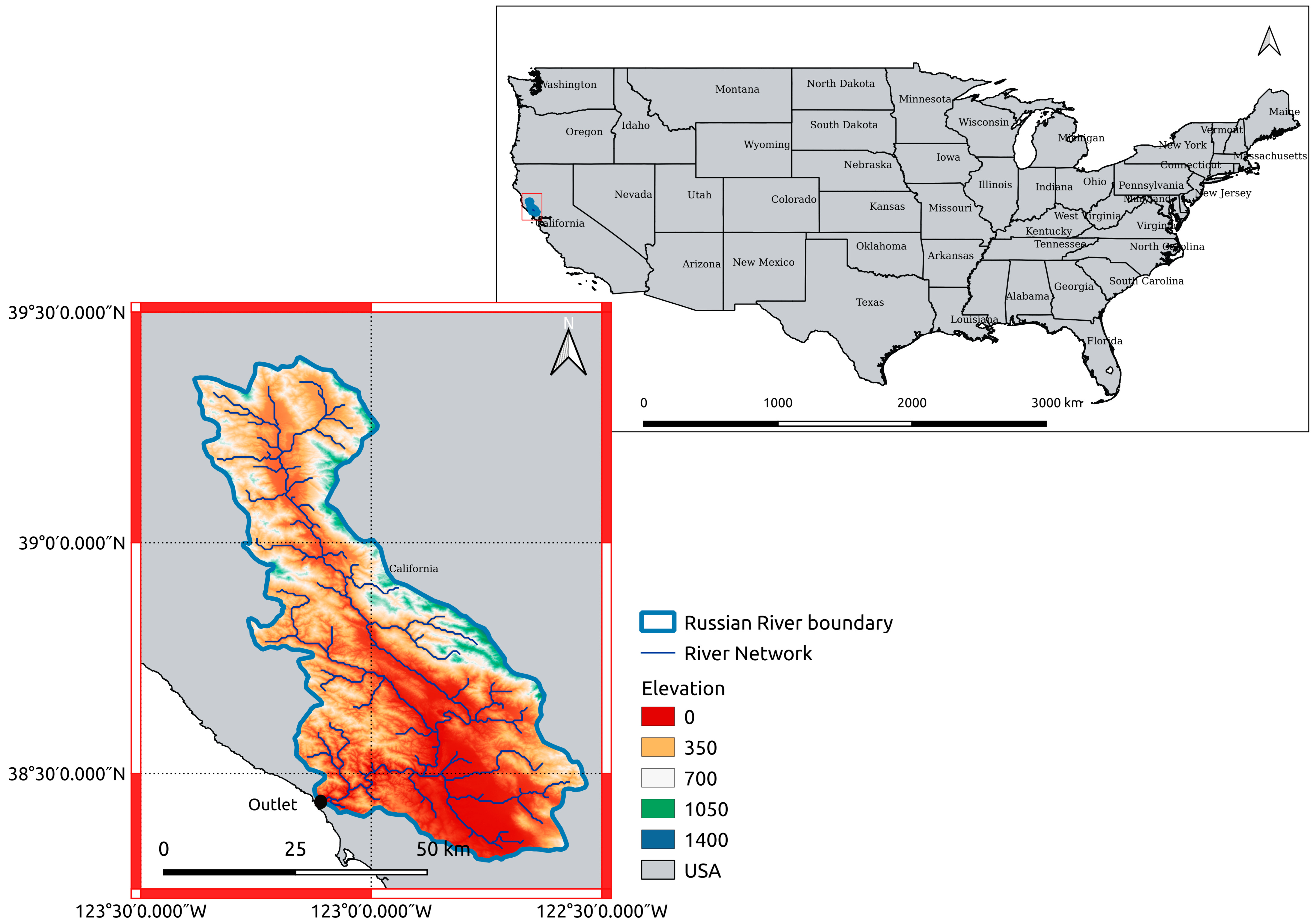
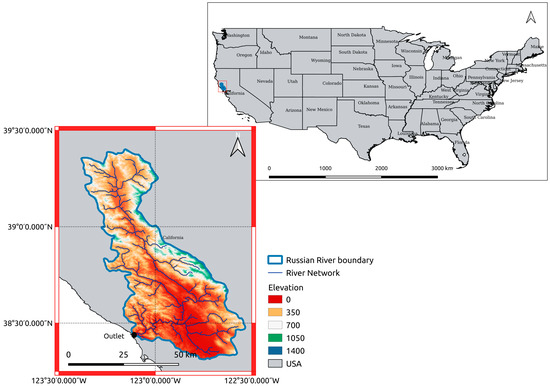 Figure 1. The study basin overlaid with an elevation map, streams, and the catchment outlet.
 - Evapotranspiration (ET): Land evapotranspiration is one of the major components of global energy, water, and biogeochemical cycles [41], and accurate estimates are critically important in hydrology, climate, and weather prediction [42]. Numerous evaluations have been performed to find the most reliable ET data worldwide (e.g., [43,44,45] and have shown that the Global Land Evaporation Amsterdam model database is highly accurate.ET is one of the outputs of the VIC model based on the Penman–Monteith equation. ET accuracy is directly related to the accuracy of data inputs to the model, especially precipitation data. Although the aim of this study was not to calibrate ET but to evaluate this output, we test how different PERSIANN family precipitation datasets affect the simulated evapotranspiration along with other model outputs. In this study, the daily data of the Global Land Evaporation Amsterdam model (GLEAM) [46] dataset with a spatial resolution of 0.25° × 0.25° is used as a reference for the evaluation of the actual ET. The GLEAM algorithm estimates land evaporation primarily based on a parameterized physical process that uses extensive independent remote-sensing observations as a basis for calculating land evaporation. Because the model is not calibrated based on ET data, the results of the ET evaluation are derived for the whole study period, i.e., from 2011 to 2018.
- Soil Moisture: we use the Soil Moisture Active Passive (SMAP) measurements as a reference for evaluating the soil moisture in the simulation. The SMAP mission of the National Aeronautics and Space Administration (NASA) was launched in 2015 [47]. This product has been evaluated and analyzed by various researchers around the world, and almost all of them emphasized that this product has the best performance among other satellite and reanalysis soil moisture data [48,49,50].While the VIC model is based on water balance and the evaluation of soil moisture data is not the main purpose of this study, it can help with examining other components of water balance. The SMAP L3 Radar/Radiometer Global Daily 9 km EASE–Grid Soil Moisture was the specific product employed. It provides soil moisture at a depth of 5 cm, which corresponds to the first layer of soil in the VIC model.
2.3. Study Area and Period
The Russian River, located in the western US in the northern latitudes 38°18′ to 39°25′ and the eastern longitudes −123°23′ to −122°32′, with a drainage area of 3850 km2, is the second-largest river flowing through the nine-county San Francisco Bay Area. It provides groundwater recharge and water supply for the agriculture sector. Figure 1 shows the location of the Russian River catchment and its main branches. Catchment elevation ranges from sea level in the southwest to 1326 m in the north and northeast. It is a rain-dominated basin with an average wintertime (December–February) temperature above 7.58 °C with dry summers and wet winters. Over 96% of the annual total precipitation falls between October and April. The average annual precipitation is 1061 mm for the period 1950–2017 [51]. Our experiment is performed using 8 years of data (2011–2018) with 5 years used for calibrating the model (2014–2018) and 3 years for validation (2011–2013). The average streamflow for both the calibration and validation periods is approximately the same, with the calibration period spanning the period for which the SMAP data are available. According to the land cover map, woody savannas and evergreen needle leaf forests classes are dominant cover, by covering 30% and more than 24%, respectively.
2.4. Evaluation Metrics
To quantitatively evaluate different precipitation products and model outputs, seven statistical metrics including the correlation coefficient (CC), root mean square error (RMSE), percentage bias (PBIAS), EKGE, probability of detection (POD), false alarm ratio (FAR), and critical success index (CSI), were selected at three temporal scales, namely daily, monthly, and seasonal. CC reflects the degree of linear correlation between the two datasets; the optimal value is 1. RMSE measures the deviation between the two datasets and describes the data dispersion degree, and PBIAS reflects system error; the optimal value for both RMSE and BIAS is 0. POD indicates the ability of precipitation products to accurately capture precipitation occurrence, with an optimal value of 1. FAR indicates the rate of incorrect precipitation occurrence prediction, with an optimal value of 0. CSI reflects the ability of the precipitation product to comprehensively detect actual rainfall events, with an optimal value of 1. Table S1 provides the formulation of all the statistical assessment criteria used in this study.
3. Results and Discussion
3.1. Evaluation of Precipitation Forcing
3.1.1. Evaluation of Climatology Datasets
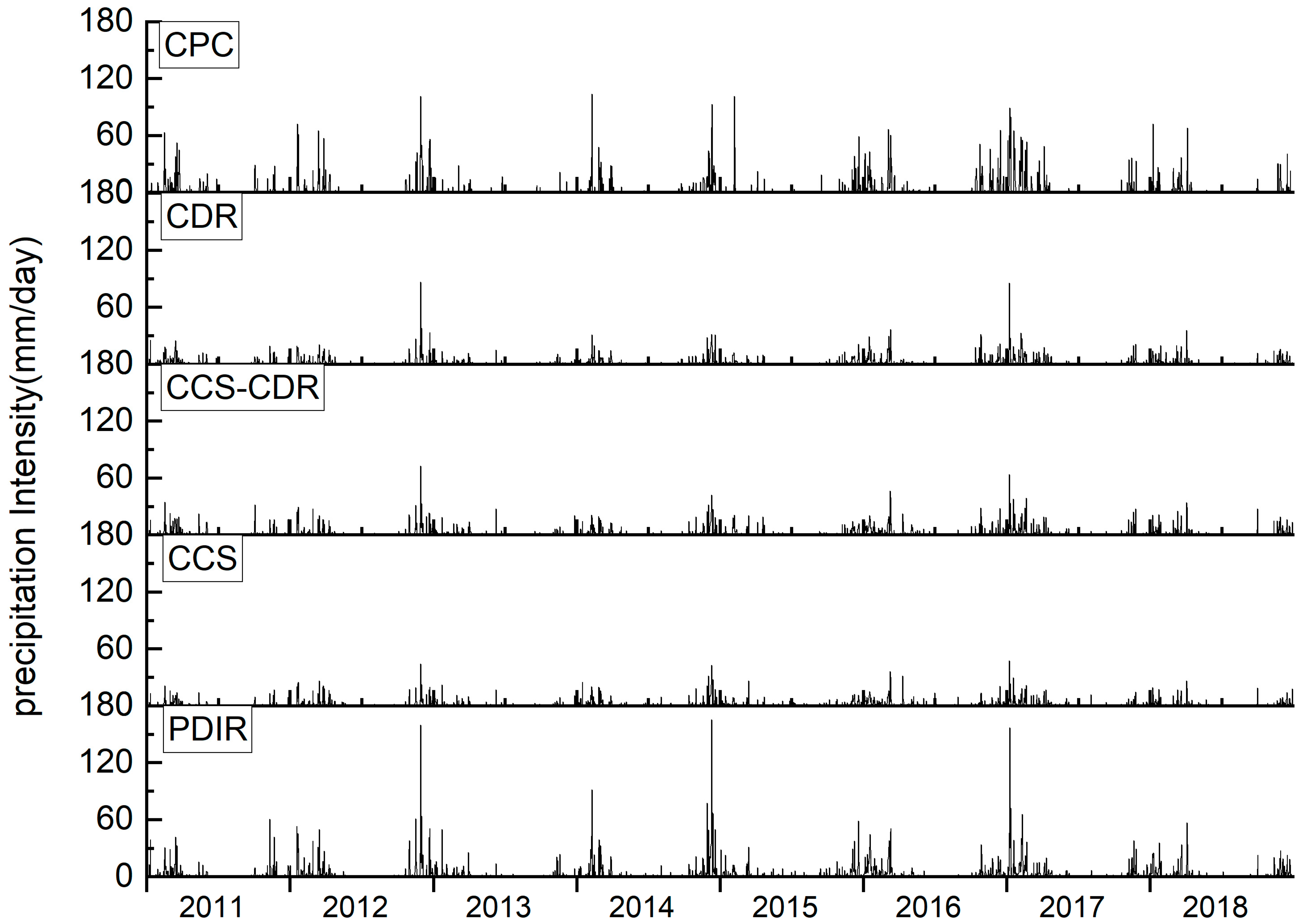
Figure 2 shows the time series of average daily precipitation over the catchment for the period 2011–2018 for each satellite-derived dataset with CPC as the reference precipitation. Visual inspection of the precipitation rates and patterns in conjunction with the quantitative statistics reported in Table 1 are used to assess agreement between satellite products and CPC. Based on CPC, the average daily precipitation in winter (December, January, and February) and summer (June, July, and August), as the wettest and driest seasons, are 4.8 mm/day and 0.39 mm/day, respectively.
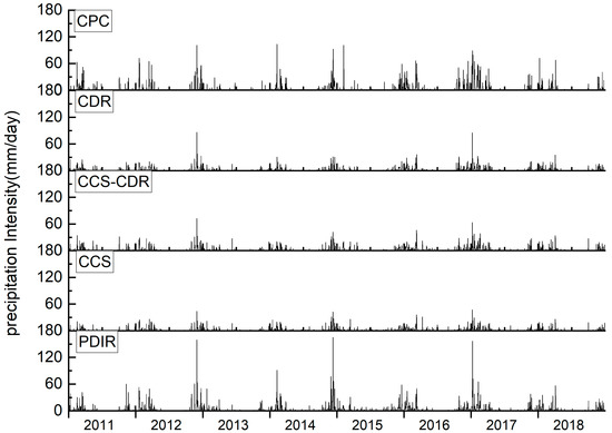
Figure 2.
Daily basin averaged precipitation time-series CPC (reference), PERSIANN–CDR, PERSIANN–CCS–CDR, PERSIANN–CCS, and PERSIANN–PDIR results.

Table 1.
Statistical summary of multiple precipitation products against CPC on daily and seasonal scales.
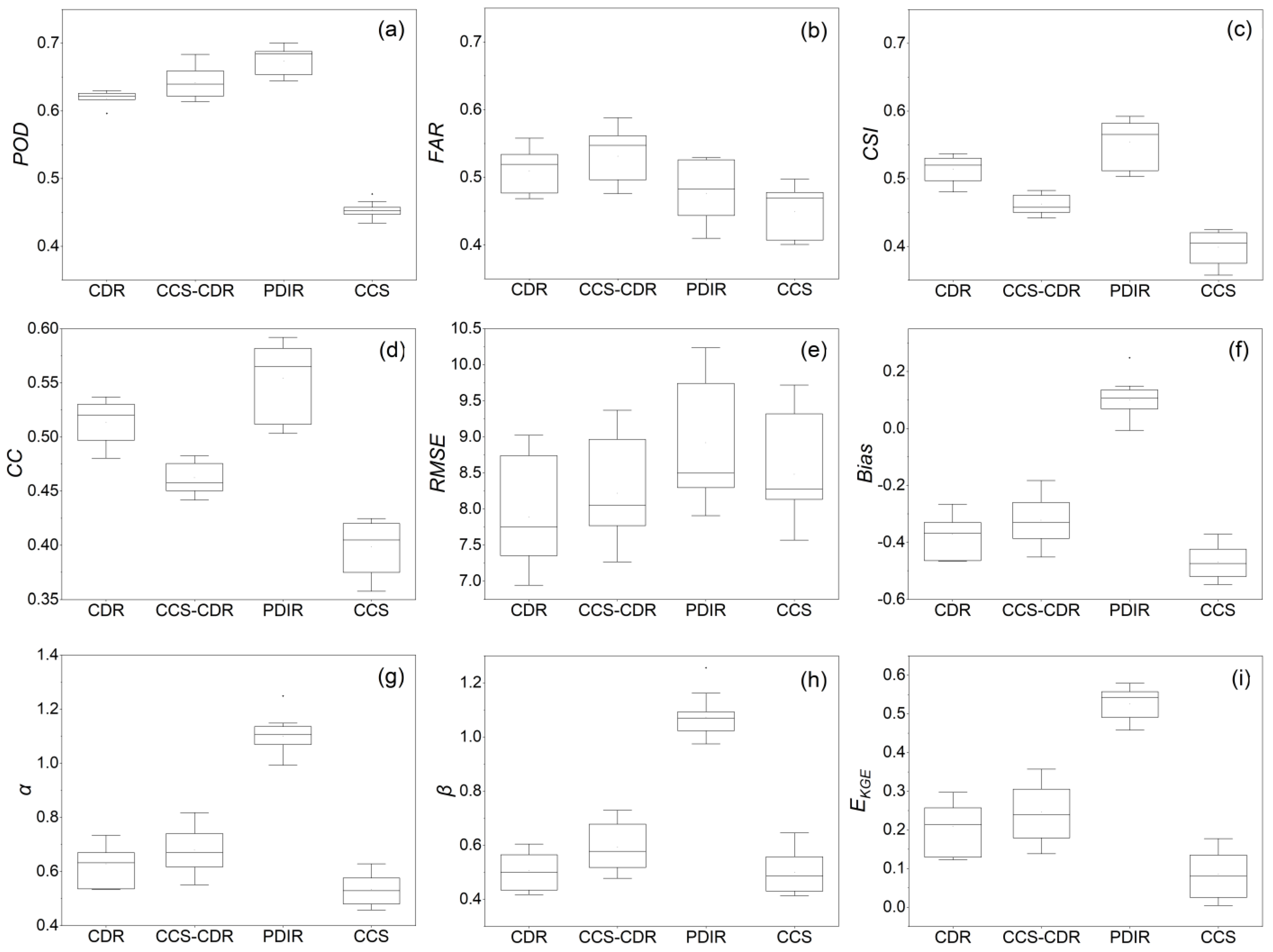
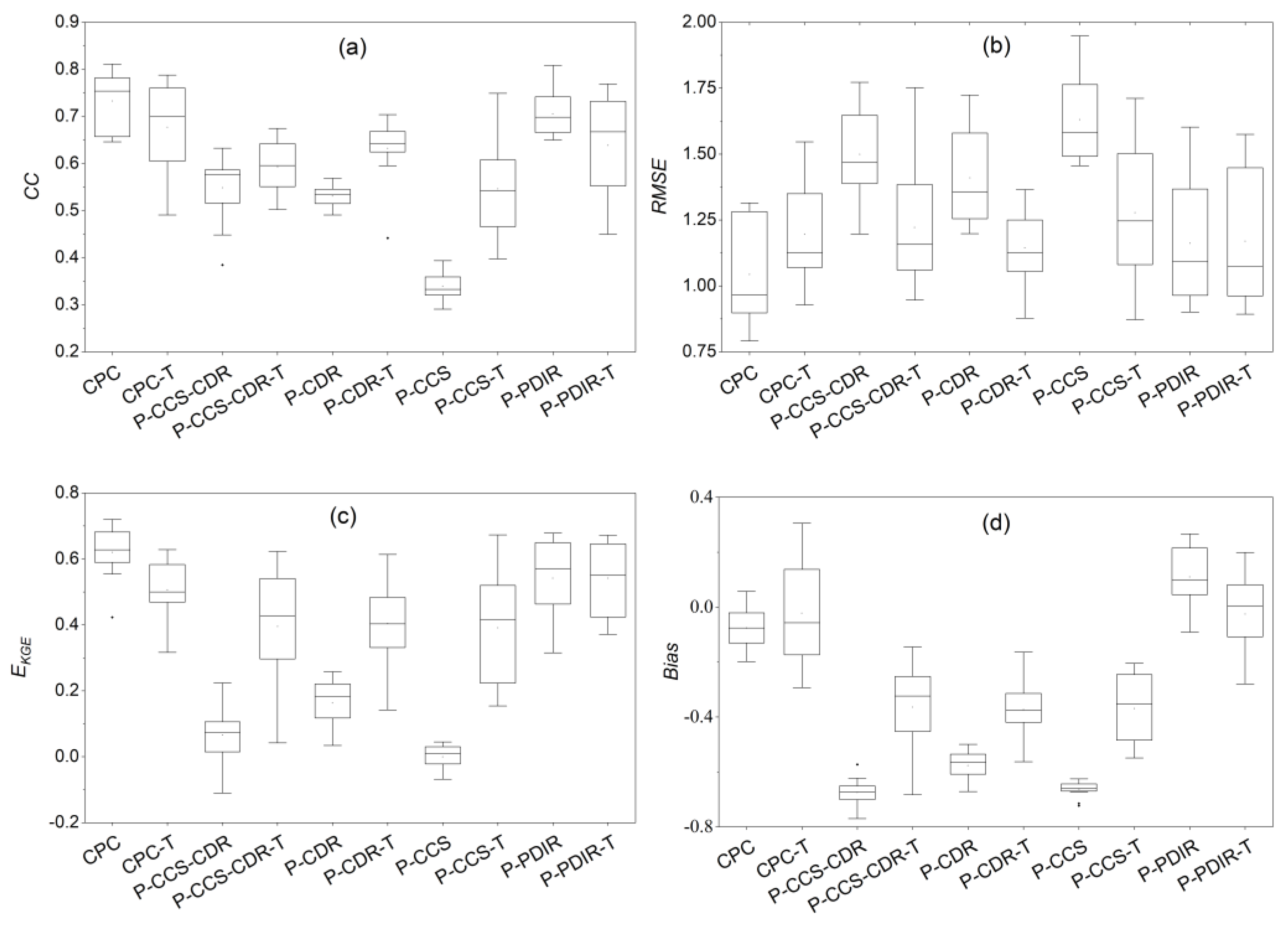
For daily precipitation, CCS–CDR outperforms CDR for some performance criteria (Figure 3 and Figure 4). For example, the Bias and POD for CCS–CDR are 0.32 and 0.64, and for CDR, they are 0.36 and 0.62, respectively. For the other criteria, CDR was better. FAR, CC and RMSE were 0.51, 0.51, and 7.90 for CDR, whereas for CCS–CDR, they were 0.53, 0.46, and 8.26. CSI and EKGE are more general performance criteria; for CSI, CDR performs better (CCS–CDR = 0.46 and CDR = 0.51), but for EKGE, CCS–CDR is better (CCS–CDR = 0.25 and CDR = 0.22). Spatial distribution of these criteria over the Russian River are presented in Figure S1.
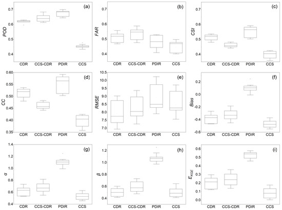
Figure 3.
The box plot of the continuous detection (POD (a), FAR (b), CSI (c)) and statistical indices (CC (d), RMSE (e), bias (f), α (g), β (h), EKGE (i)) for the evaluation of the PERSIANN family over the Russian River basin using CPC as the reference.
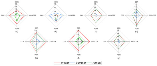
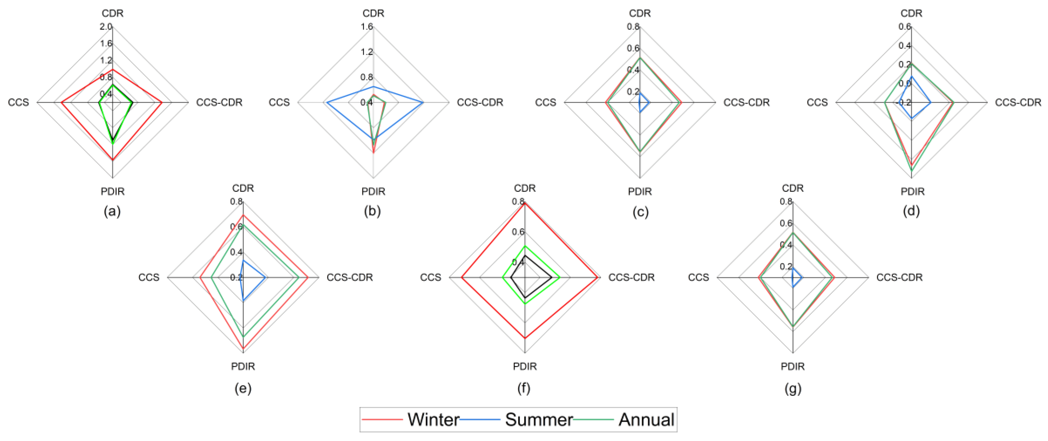
Figure 4.
The average of the statistical (α (a), β (b), CC (c), EKGE (d)) and detection (POD (e), FAR (f), CSI (g)) indices for the studied PERSIANN family over the Russian River basin.
On a seasonal scale such as the whole period throughout the 8 years, the performance of these two datasets can be examined from different aspects. According to Figure 4, in winter, POD, Bias, and EKGE for CCS–CDR were 0.71, 0.35, and 0.24, while for CDR the equivalent scores were 0.70, 0.38, and 0.21. CDR was better according to CC, RMSE, FAR, and CSI, which were 0.52, 10.98, 0.44, and 0.45, with CCS–CDR returning 0.48, 11.29, 0.47, and 0.45, respectively. Both datasets show the best performance in winter. In summer, CDR outperformed CCS–CDR for most performance criteria. For example, RMSE, Bias, CC, and EKGE were 2.06, 0.03, 0.19 and 0.08 for CDR, while the equivalent scores for CCS–CDR were 2.44, 0.41, 0.18, and 0.0. The newest dataset had slightly better performance at detecting precipitation occurrence where POD, FAR, and CSI were 0.39, 0.78, and 0.17 for CCS–CDR and 0.36, 0.79, and 0.16 for CDR. On a monthly scale, CCS–CDR was better on all performance criteria except CC, where CCS–CDR was 0.94 and CDR was 0.96. For CCS–CDR, Bias, RMSE, and EKGE were 0.32, 65.88, and 0.43, while for CDR, they were 0.35, 67.18, and 0.39. As evaluated against CPC, it can be concluded that CCS–CDR performed better in POD well as Bias, while CDR had a smaller FAR and more correlation. These results are consistent with the findings of Sadeghi et al. (2021) and Huang et al. (2021), who find that the rate of Bias and RMSE in CCS–CDR has decreased significantly throughout the whole period as well as wet seasons and heavy rainfall events [12,52].
3.1.2. Evaluation of Near-Real-Time Datasets
According to Table 1 and Figure 4, PDIR was better at detecting precipitation events (POD: CCS = 0.45 and PDIR = 0.67), but CCS has fewer false alarms based on FAR (CCS = 0.45, PDIR = 0.48). CSI criteria show that PDIR is more reliable than CCS in detecting the precipitation events (CCS = 0.40 and PDIR = 0.55). Bias, CC, and EKGE scores are substantially better for PDIR than CCS (PDIR: 0.09, 0.56, 0.53 and CCS: −0.47, 0.38, and 0.08, respectively). Although CCS is better for RMSE (CCS = 8.59 and PDIR = 8.86 mm), PDIR is significantly better than CCS overall.
In winter, the superiority of PDIR is notable, especially for EKGE, which is 0.46 for PDIR and 0.08 for CCS. PDIR has better precipitation detection accuracy for all skill scores (see Figure 4 and Table 1). Both datasets have the worst performance in summer, but PDIR is still more reliable than CCS. For example, POD is 0.38 for PDIR and 0.22 for CCS, and CC is 0.19 and 0.11 for PDIR and CCS, respectively. These results have agreement with the findings of Saemian et al. (2021), who found that the rate of EKGE and CC in PDIR increased significantly and the rate of Bias decreased [53]. In additional confirmation of the findings of this study, the results of Huang et al. (2021) showed that PDIR had better performance in detecting rainfall events and fewer false alarms.
3.2. Evaluation of Streamflow Simulations
We calibrated the model in nontransformation and Box–Cox transformation, with results presented separately. Optimum parameters are presented in Table S2 for each dataset and calibration mode.
3.2.1. Evaluating Streamflow in Nontransformation Mode
First, the CPC dataset was used to run the VIC model for the Russian River basin before each of the PERSIANN precipitation products was used in turn. Time series of daily streamflow hydrographs simulated from the CPC and PERSIANN products are illustrated in Figure 5 and Figure 6 for the calibration and validation periods. Figures S2 and S3 show scatter plots of the simulated daily streamflow using different precipitation products as the inputs of the VIC model. Based on these figures and Table 2, it can be seen that the VIC model run with CPC as the input has high skill at simulating streamflow in the Russian River basin. The daily EKGE is 0.75 in the calibration period and 0.76 in the validation period (Table 2). In winter, EKGE in the calibration period is 0.74 and is 0.76 for validation, indicating that the model has good performance in estimating high flows (Figure 5 and Figure 7). Table 2 show EKGE scores for monthly data during the calibration and validation periods, with EKGE scores of 0.62 and 0.93. The evaluation of streamflow simulation results using CPC dataset showed that although based on station data, it did not provide accurate results for several peak discharges. This may be due to uncertainty in the model structure, model parameters, inputs and the observational data [54]. These results help to better understand the hydrologic model’s ability to simulate streamflow and provide good criteria for general insights on error related to PERSIANN precipitation products and VIC hydrology.
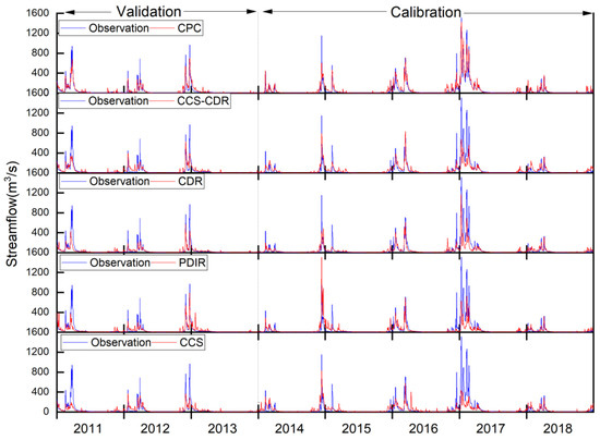
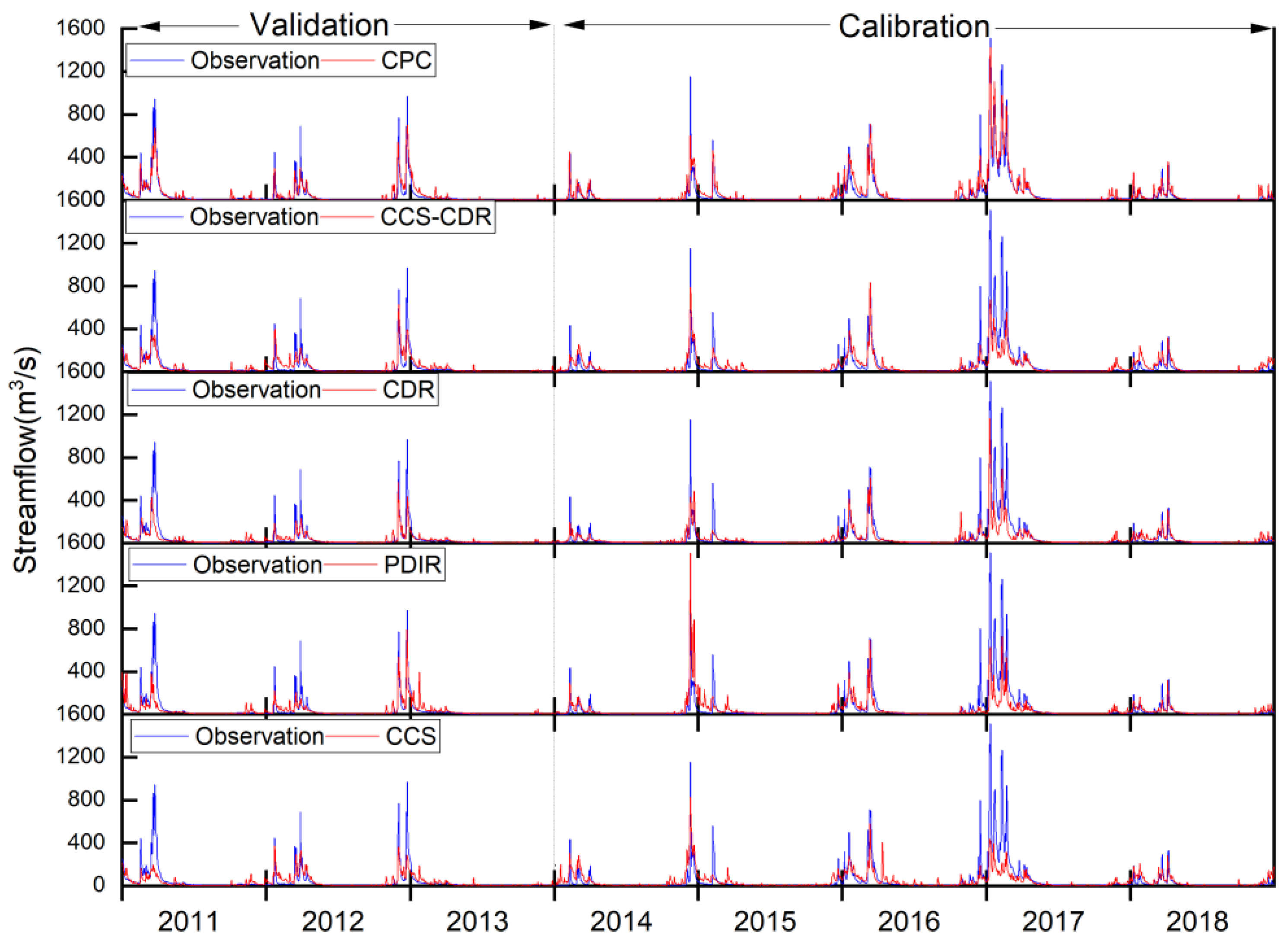
Figure 5.
Daily streamflow hydrographs generated from CPC and the PERSIANN family.
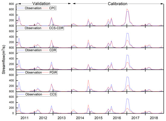
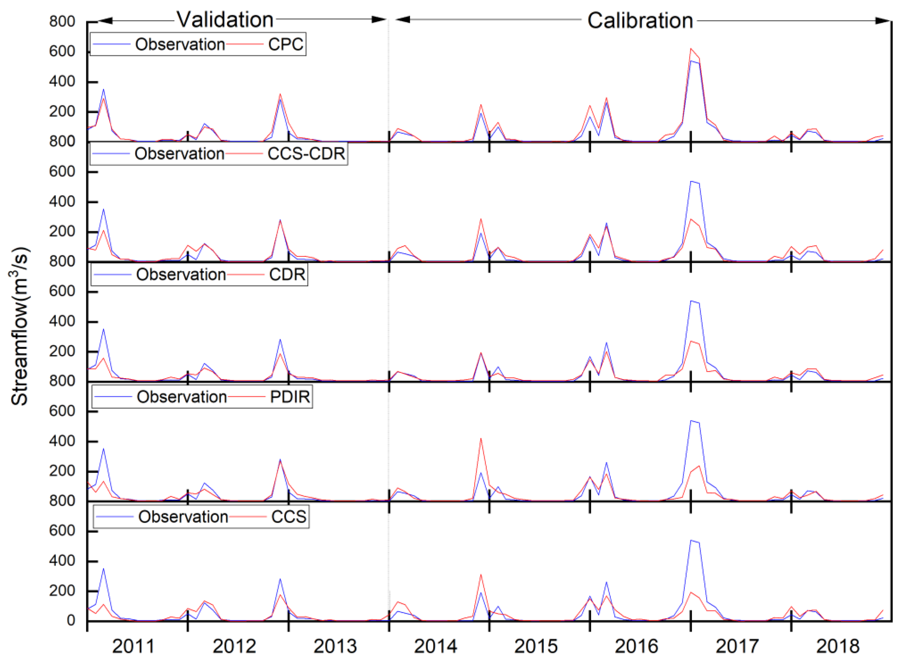
Figure 6.
Monthly streamflow hydrographs generated from CPC and the PERSIANN family.
Table 2.
The performances of streamflow simulations driven by CPC and PERSIANN family precipitation dataset on a daily, winter, and monthly scale.
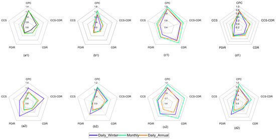
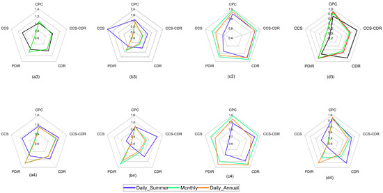
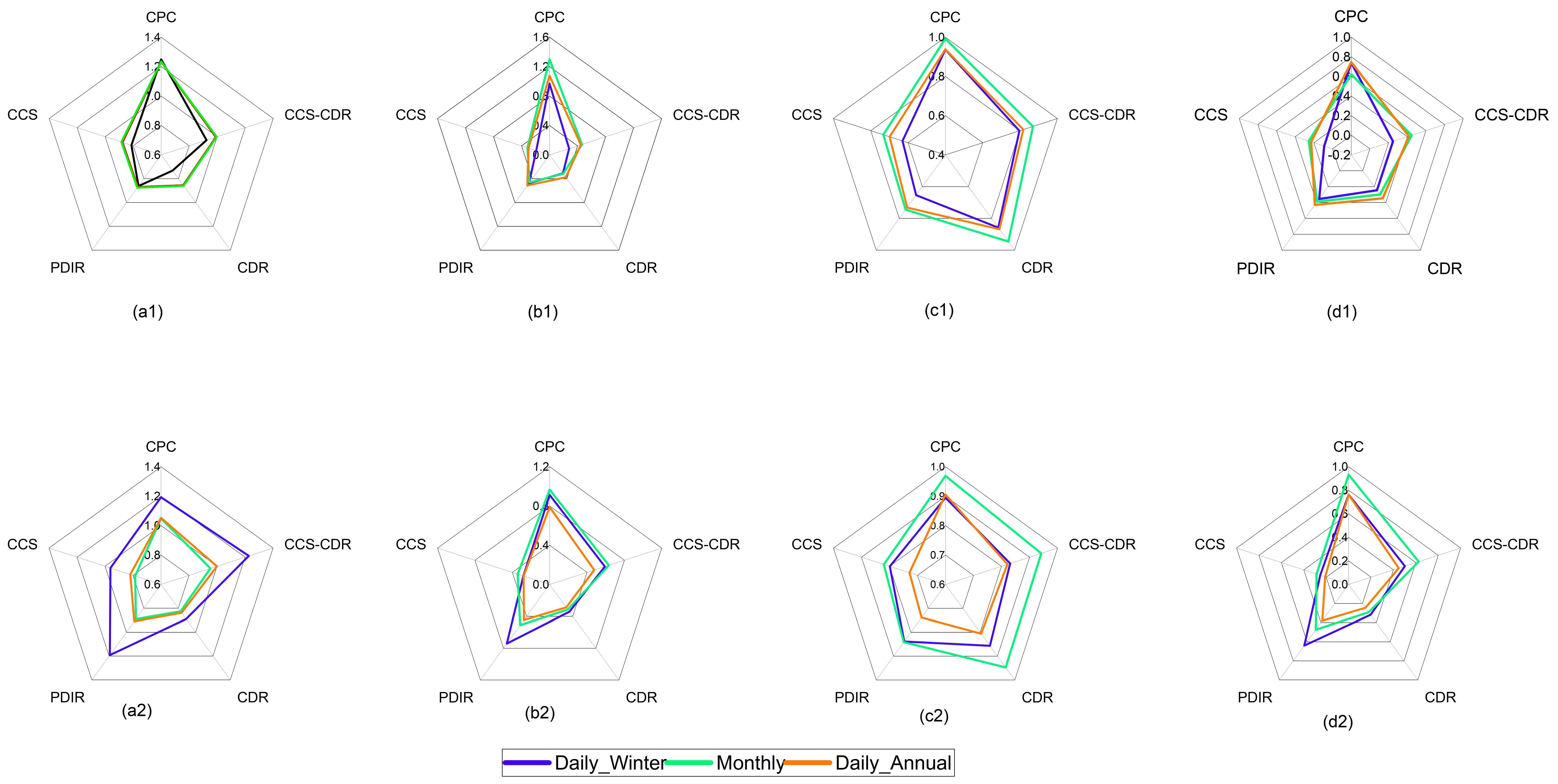
Figure 7.
The results of EKGE and its components for simulating the runoff using CPC and PERSIANN family datasets. In the nontransformed calibration process: α (a1), β (b1), CC (c1), and EKGE (d1) for calibration period and α (a2), β (b2), CC (c2), and EKGE (d2) for validation periods at daily and monthly scales and winter. In the transformed calibration process: α (a3), β (b3), CC (c3), and EKGE (d3) for the calibration period and α (a4), β (b4), CC (c4), and EKGE (d4) for the validation period at daily and monthly scales and summer.
Figure 5 and Figure 6 show that the simulated runoff using CDR and CCS–CDR are similar. In the calibration and validation periods, CCS–CDR outperforms CDR with our objective function (EKGE 0.42 and 0.44 for CCS–CDR and 0.35 and 0.24 for CDR, respectively). The reason for the superiority of CCS–CDR is that it has a significantly better mean than CDR, while CDR shows a better correlation, although this advantage is not significant (Figure 7). Both datasets fail to capture the heavy precipitation in January and February 2017, and as a result, generated runoff from the VIC model shows weak performance for this event. During validation, CCS–CDR showed improved performance relative to calibration, while the accuracy of CDR decreases compared with the calibration period. In the validation period, CCS–CDR better simulates peak discharges, especially at the end of 2012. Figure 4 shows that CDR usually underestimates peak flows, while CCS–CDR both over- and underestimates different peak flows. This might be the result of using daily forcing data and consequently missing the actual intensity of the precipitation at finer temporal scales. CCS–CDR has hourly data, but as the aim of the present study is to compare different PERSIANN products with CDR, we applied data with daily time step. During the wet winter season, the performance of CCS–CDR and CDR are the same based on EKGE (CDR: 0.25, CCS–CDR: 0.25). However, in the validation period, CCS–CDR shows better performance (CDR: 0.32, CCS–CDR: 0.50), although it still underestimates the flow values. CDR shows a higher correlation with the observed runoff during calibration (CDR: 0.86, CCS–CDR: 0.80) and validation (CDR: 0.86, CCS–CDR: 0.83). The superior correlation for CDR was also observed in the precipitation evaluation.
Assessing the performance of the CDR and CCS–CDR datasets in the simulation of monthly streamflow is important because these two datasets have longer historical records and have had more applications in climatic science. Monthly results are evaluated with and without transformation. CCS–CDR performs better for monthly runoff simulations (Figure 6 and Table 2), with EKGE for the calibration and validation periods for CCS–CDR being 0.45 and 0.65, while for CDR, the equivalent values are 0.30 and 0.29.
As was shown in the precipitation analyses, PDIR performs better than CCS, which is the case in streamflow simulation. During the calibration period, PDIR estimates runoff more accurately, with EKGE scores of 0.43 and 0.23 for PDIR and CCS, respectively. Based on the correlation coefficient, PDIR is again slightly better, with CC of 0.73 and 0.70 for PDIR and CCS, respectively. The largest difference between the two datasets is in runoff simulation at the beginning of 2017, where PDIR performs similarly to CDR and CCS–CDR but CCS performs very poorly. The largest difference in runoff estimation occurred on 12 December 2014, with an observed daily discharge of 1151 (m3/s), but the PDIR overestimated it at 1528 (m3/s). During the validation period, the performance of both datasets reduced relative to the calibration period. EKGE in this period is 0.38 for PDIR and 0.21 for CCS. Figure 7 shows the results of these two datasets for the entire simulation period and over the winter for the calibration and validation periods. CCS always underestimates runoff, which is consistent with the results of the precipitation evaluation. PDIR has intermittent behavior, with frequent periods of overestimation/underestimation. Winter simulation results again show more accurate runoff simulations using PDIR during both the calibration and validation periods. In terms of correlation, PDIR is better in the calibration period, but in the validation period, the two have the same performance. EKGE in the two periods is 0.36 and 0.64 for PDIR and 0.09 and 0.25 for CCS. PDIR has the best performance among the PERSIANN family dataset in winter. According to Table 2 and Figure 6, the performance of two near-real-time datasets on a daily scale is replicated on a monthly scale, and just as PDIR was superior on a daily scale, it performs better and is more reliable on a monthly scale. In the calibration and validation periods, EKGE is 0.39 and 0.47 for PDIR and 0.26 and 0.30 for CCS. Considering these differences and the advantages of each of these datasets, to choose a more efficient database, one should review the conditions of the basin under study and the study period. The superiority of PDIR over CCS is quite evident in terms of the accuracy of both precipitation and simulated streamflow, especially in wet seasons, which could be a great advantage in flood estimation and warning systems.
3.2.2. The Evaluation of Streamflow in Transformation Mode
This acceptable performance for CPC in the nontransformation state is repeated in the transformed state, where the values of EKGE are equal to 0.86 and 0.92 in the calibration and validation periods, respectively. In summer, based on Box–Cox transformed flows, EKGE during calibration was 0.71 and 0.87 for the validation period (Figure 5 and Table 3). EKGE at monthly scale, shown in Table 3, is 0.91 and 0.92 during the calibration and validation periods, respectively. These results show that the VIC hydrological model and CPC dataset are skillful in simulating the low flow in the Russian River catchment. Figure 8 and Figure 9 show the simulated runoff using CPC and PERSIANN family precipitation datasets with Box–Cox transformation.
Table 3.
The performances of streamflow simulations driven by CPC and PERSIANN family precipitation dataset at daily, summer, and monthly scale with Box–Cox transformation.
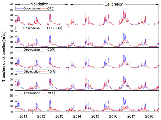
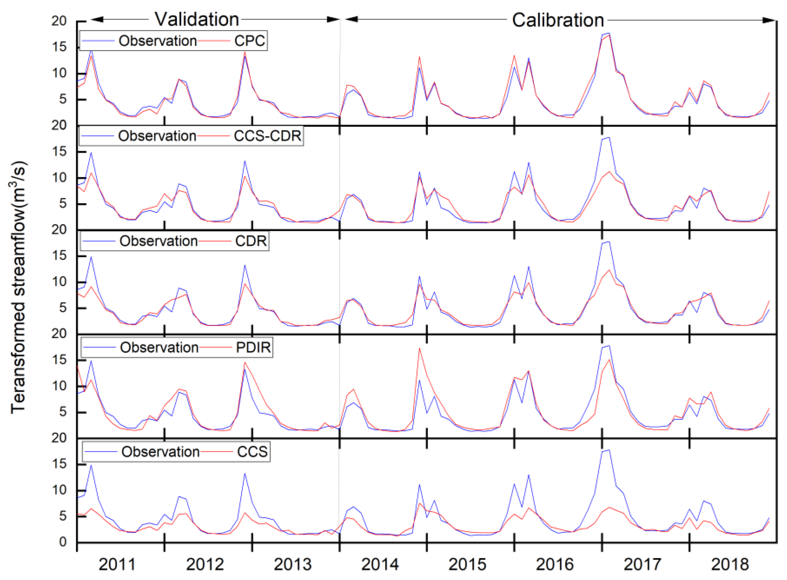
Figure 8.
Daily transformed streamflow hydrographs generated from CPC and the PERSIANN family.
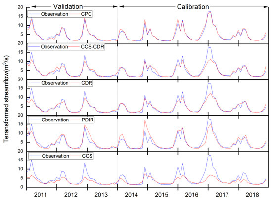
Figure 9.
Monthly transformed streamflow hydrographs generated from CPC and the PERSIANN family.
EKGE as an objective function and its component are show, in Table 3 and Figure 7. During the calibration period, CCS–CDR has slightly better performance than CDR (CDR: 0.47 and CCS–CDR: 0.51), and this advantage was repeated with more differences during the validation period (CDR: 0.45 and CCS–CDR: 0.57). In the dry summer season, CCS–CDR is better in the calibration period (CDR: 0.85 and CCS–CDR: 0.82), but in validation, the performance of CCS–CDR drops (CDR: 0.83 and CCS–CDR: 0.70). Both datasets perform better than CPC in summer during the calibration period, indicating their utility for simulating low flows (see Figure S3). Regarding the CDR, it can be said that it had significant performance in dry seasons with low flows [55], and consequently, it performed better than CPC in summer streamflow simulation. The main reason CDR excels in summer is that it better captures average flows, which is related to the better Bias in precipitation evaluation. Additionally at monthly scale, EKGE for CCS–CDR is 0.56 and 0.53 for CDR during the calibration period and 0.67 and 0.53 for these datasets during the validation periods, respectively (see Figure 9 and Figure S3).
For low flows (using Box–Cox transformation), PDIR has good performance. In the calibration period, EKGE for PDIR is 0.83, with CCS showing much weaker performance (0.12). This advantage is repeated during validation (EKGE: 0.82 and 0.14 for PDIR and CCS, respectively). In summer during the calibration period, PDIR performs well according to EKGE (0.62), while this index is negative for CCS (−0.05). The performance of the two datasets is more different in the validation period, where EKGE for CCS and PDIR are 0.4 and 0.2, respectively; the main reason for the improvement of CCS relates to the closer standard deviation to the observed one. PDIR also has the best performance among the PERISANN family with applied Box–Cox transformation at monthly scale (Figure 9). EKGE for PDIR is 0.84 and 0.61 for calibration and validation, while for CCS, the equivalent results are 0.12 and 0.14, respectively.
Various researchers have used positive EKGE values as indicative of “good” model simulations, whereas negative EKGE values are considered unsatisfactory, without explicitly indicating that they treat EKGE = 0 as their threshold between good and bad performance [56,57,58]. Therefore, the modeling results in this study are “skillful” (except for CCS in summer).
3.3. Evaluation of Evapotranspiration
Figure 10 shows the performance of the VIC model in simulating ET in terms of CC (a), RMSE (b) EKGE (c), and Bias (d) using different PERSIANN products. The CPC dataset had a higher correlation (CC = 0.73) compared with CPC–T (CC = 0.68), while based on the average of Bias, both CPC and CPC-T slightly underestimated the ET, the RMSE, and EKGE; that is, CPC outperforms CPC-T. According to Figures S5 and S6, which show the spatial distribution of the evaluation criteria, CPC was better in the center of the catchment, with higher CC and EKGE and lower RMSE and Bias, while CPC-T was better in these criteria.


Figure 10.
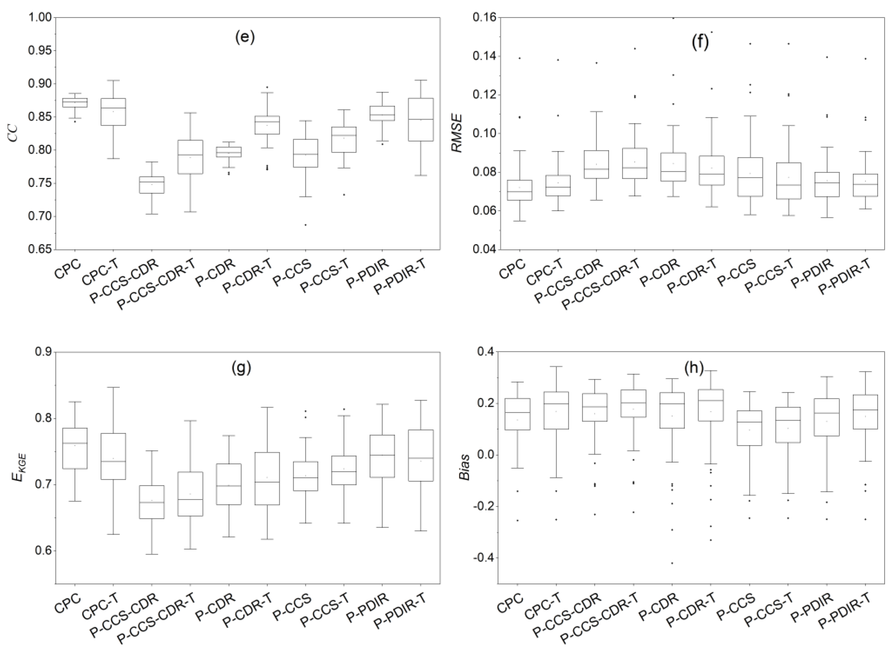
The box plot of the continuous CC (a), RMSE (b), EKGE (c), and Bias (d) for the evaluation of ET using CPC and the PERSIANN family over the Russian River basin and using the GLEAM as reference and the CC (e), RMSE (f), EKGE (g), and Bias (h) for the evaluation of soil moisture using CPC and the PERSIANN family and the SMAP as reference.
The CCS–CDR and CDR datasets have same behavior in simulating the ET. The results of the ET evaluation of the model output show that the calibration of the model with Box-Cox transformation leads to better results in ET simulation; therefore, we analyze the result of calibration with transformation. According to Figure 10a, the CDR-T dataset had higher correlation (CC = 0.63) than CCS–CDR-T (CC = 0.59). Average Bias is negative and the same for these datasets (Bias: CCS–CDR-T: −0.37 and CDR-T: −0.38), which is consistent with the negative Bias in rainfall and runoff. EKGE is also very close: 0.39 and 0.4 for CCS–CDR-T and CDR-T, respectively. Figures S5 and S6 show that RMSE in CCS–CDR-T and CDR-T decrease from north to south. This reduction in error for CCS–CDR-T also applies to Bias but not in CDR-T. CC and EKGE for CCS–CDR increase from north to south, but as shown in Figure 10, the amplitude of the CDR-T changes is smaller than that of CCS–CDR-T and has a similar performance across the catchment.
According to Figure 10 and based on EKGE, both near-real-time datasets better estimate evapotranspiration in calibration mode with transform, and therefore, we used these results for analysis. In the whole period, PDIR-T had better correlation than CCS-T (CC: CCS-T = 0.55, PDIR-T = 0.64), and PDIR is obviously better in Bias (Bias: CCS-T = −0.37 and PDIR-T = −0.03). These superiorities give even better EKGE results (EKGE: CCS-T = 0.39 and PDIR-T = 0.54) and are RMSE (RMSE: CCS-T = 1.28, PDIR-T = 1.17 mm). From the spatial distributions of these criteria, which are shown in Figures S5 and S6, it can be concluded that these two datasets, similar CPC and CCS–CDR-T, have better performance in the south than in the north, which can be attributed to vegetation characteristics and factors affecting evapotranspiration.
Regarding the overall performance of the datasets in ET simulation throughout the modeling period, the best performance related to CPC, followed by PDIR. Although these results are not the best possible results because the model is not calibrated based on evapotranspiration, it can be concluded that all these datasets can simulate evapotranspiration at an acceptable level. However, to obtain better results, the dataset should be selected based on the purpose of the research.
The results show although we did not calibrate the model for ET, all datasets had the ability to spatially simulate ET in an acceptable way. Based on EKGE, CCS–CDR and CDR datasets simulated ET better than the CPC dataset, and CCS had the best performance in winters. The difference in performance over various seasons is due to the different performances of these precipitation datasets along with the philosophy behind the development of these datasets; hence, to obtain the best result, an appropriate product should be selected based on the simulation purpose.
3.4. Evaluation of Soil Moisture
Figure 10 shows the performance of the VIC model in simulating soil moisture in terms of CC (e), RMSE (f), EKGE (g), and Bias (h) using different PERSIANN products, and Figures S7 and S8 show the spatial distribution of these criteria over the Russian River catchment.
Figure 10e shows the distribution of CC in all basin grids based on SMAP grid size. It can be seen that all datasets show a correlation above 0.75. CPC followed by PDIR shows the highest correlation among simulated results, with average correlations of 0.87 and 0.85, respectively. Another near-real-time dataset has performance close to PDIR, with an average correlation of 0.79. Among climatic datasets, the CDR shows better correlation with an average value of 0.8, while the mean correlation for CCS–CDR for all grids is 0.75. These results are related to the nontransformed datasets, but the results of calibration with the transformed datasets are very close to the original datasets.
The results for RMSE are presented in Figure 10f. The best performance related to the CPC dataset, with RMSE of 0.07 for both the transformed and nontransformed datasets. The average RMSE for all datasets is very similar in in terms of transformed and nontransformed modes. Overall, the two near-real-time datasets are slightly better for PDIR, which has less RMSE error. CCS–CDR and CDR have the same performance according to this criterion.
Figure 10g provides the EKGE, which is very close for CCS–CDR and CDR in nontransformed and transformed modes: 0.68 and 0.7 and 0.69 and 0.71 for this products, respectively. Among the near-real-time datasets, just as it outperformed PDIR in assessing rainfall accuracy and runoff simulation, CCS–CDR performed better, with mean EKGE of 0.74, while this criterion was 0.71 for CCS. EKGE for both calibration processes are the same for these two datasets, although their performance is different in different cells. The mean EKGE for the nontransformed and transformed CPC datasets is 0.76 and 0.74, respectively, not significantly different from the PDIR dataset.
The average Bias, presented in Figure 10h, is positive for all datasets; this indicates that all datasets estimate soil moisture above the actual level. CCS have the best performance in both nontransformed and transformed modes (Bias = 0.13). Following this dataset, the other near-real-time dataset performed better, with average Bias of 0.15, which was even better than the CPC average of 0.16. CCS–CDR and CDR have very close, Bias, but CCS–CDR is better with (Bias: CCS–CDR = 0.19 and CDR = 0.2).
Based on Figures S7 and S8, it can be concluded that the performance of all datasets is better in the north and west and worse in the east and center regions of the basin. The CPC dataset has almost the same performance throughout the basin except for the middle and east of the basin. CCS–CDR and CDR are almost identical in terms of spatial distribution, especially in the northern areas and the outlet of the basin. These datasets are similar in the spatial distribution of the evaluation criteria. Between the two near-real-time datasets, the PDIR dataset performs better in the border areas, and this advantage is more evident in the output and southern parts of the basin. However, there is no significant difference in the CCS dataset, and we can only say that it performs more satisfactorily in the northern half than in the southern parts. The common denominator of soil moisture simulation is that all datasets in the southwest of the basin, which is the outlet of the basin, underestimate soil moisture.
The maximum and minimum EKGE were 0.76 and 0.68 in CCS–CDR, respectively, without any significant difference from the CPC results, especially the PDIR results, which were similar to CPC. It should be noted that the results are based on runoff calibration and accuracy could improve with a focus on ET and soil moisture calibration.
4. Conclusions
Although many studies have examined the performance of the CCS and CDR datasets so far, we used these two datasets in addition to the CCS–CDR and PDIR datasets to investigate the applications of PERSIANN family datasets in hydrological models and compare the ability of new and old versions of the CHRS.
The results showed that the CCS–CDR had less Bias than its predecessor, i.e., CDR. CCS–CDR performed better in wet seasons, while CDR is better in dry seasons. Evaluation of near-real-time precipitation datasets showed that the PDIR performed significantly better than CCS. PDIR performed much better in detecting rainfall events and is more reliable than CCS in wet seasons. While CCS–CDR, CDR, and CCS datasets underestimates, PDIR performs differently from other PERSIANN family databases and overestimates.
Evaluating the applications of the PERSIANN family for hydrological modeling showed the efficiency of these products in simulating the streamflow. We calibrated the model using two methods, i.e., based on nontransformed (original) datasets and with Box-Cox transformation. In the first calibration method, which focuses on high flow, CCS–CDR and PDIR showed better performance. In the second calibration process with Box-Cox transformation, the CDR precipitation dataset was better than CCS–CDR during summer. Throughout the whole period, PDIR performed better than CCS in both the calibration and validation periods.
These results show that the ET simulated by CPC is better with the nontransformed dataset, but CCS–CDR, CDR, PDIR, and CCS revealed comparable results with better performance in estimating ET with the model calibrated by Box-Cox transformation. The best result in the whole period was related to CPC, and then PDIR-T performed better than the other datasets. CDR-T and CCS–CDR-T were better in summer, while CCS-T was the best dataset in winter. In this study, daily data were used to simulate runoff for a fair comparison between different products, and the model was calibrated with these data. Based on simulated daily evapotranspiration from the model, if the hourly data are used as input and the calibration focuses on these data, the results will be improved.
The results for soil moisture simulation showed that all precipitation data of the PERSIANN family have a high ability to simulate soil moisture, especially the PDIR dataset, with very similar results to CPC. Because the SMAP soil moisture dataset is not available in the long term and its available period is incomplete, it is possible with focus on soil moisture calibration using PERSIANN family precipitation datasets in ungauged areas to achieve a long-term and complete soil moisture dataset.
The results of this study showed that each of the PERSIANN family datasets has a special ability. CCS–CDR has better ability to simulate streamflow in winter, while CDR has better performance in simulating low flow in summer, even better than the CPC dataset. PDIR also performs better at detecting precipitation events than the CCS and in simulating streamflow in winter, while CCS can perform well at simulating low flows. These capabilities can be different depending on the period and case of study, so evaluations should be done based on the purpose of the study, and then the most efficient dataset should be selected.
Supplementary Materials
The following supporting information can be downloaded at: https://www.mdpi.com/article/10.3390/rs14153675/s1, Table S1. Statistical metrics used for evaluating multiple precipitation products; Table S2. Calibration parameter and their intervals (N: for nontransformed mode and T: for transformed mode); Figure S1. Distribution of PERSIANN family precipitation datasets performance against CPC according to EKGE (row 1 to 3 in Daily, Summer and Winter respectively) and CSI (row 4 to 6 in Daily, Summer and Winter respectively) (CDR, CCS–CDR, PDIR and CCS, column 1 to 5); Figure. S2. Scatter plot for daily streamflow generated from CPC and PERSIANN family. The horizontal axis is observation discharge (m3/s) and the vertical axis is simulated discharge (m3/s); Figure S3. Scatter plot for transformed daily streamflow generated from CPC and PERSIANN family. The horizontal axis is observation discharge (m3/s) and the vertical axis is simulated dis-charge (m3/s); Figure S4. Scatter plot monthly streamflow for general (column 1 and 2) and transformed (column 3 and 4) generated from CPC and PERSIANN family. The horizontal axis is observation discharge and the vertical axis is simulated discharge; Figure S5. CC, EKGE, RMSE and Bias (column 1 to 4) of CPC, CCS–CDR, CDR, PDIR and CCS (row 1 to 5), over the Russian River catchment for ET simulation; Figure S6. CC, EKGE, RMSE and Bias (column 1 to 4) of CPC-T, CCS–CDR-T, CDR-T, PDIR-T and CCS-T (row 1 to 5), over the Russian River catchment for ET simulation; Figure S7. CC, EKGE, RMSE and Bias (column 1 to 4) of CPC, CCS–CDR, CDR, PDIR and CCS (row 1 to 5), over the Russian River catchment for Soil moisture simulation; Figure S8. CC, EKGE, RMSE and Bias (column 1 to 4) of CPC-T, CCS–CDR-T, CDR-T, PDIR-T and CCS-T (row 1 to 5), over the Russian River catchment for Soil moisture simulation.
Author Contributions
Conceptualization, H.S., M.S., S.G. and S.S.; methodology, H.S. and M.S.; software, H.S.; validation, H.S. and M.S.; formal analysis, H.S.; investigation, H.S., M.S. and S.G.; resources, H.S., S.G., C.M. and P.N.; data curation, H.S.; writing—original draft preparation, H.S. and C.M.; visualization, H.S.; supervision, S.G., P.N. and S.S.; project administration, H.S.; funding acquisition, S.S. All authors have read and agreed to the published version of the manuscript.
Funding
The research was partially funded by the Center for Western Weather and Water Extremes (CW3E) at the Scripps Institution of Oceanography via AR Program Phase II grant 4600013361 sponsored by the California Department of Water Resources and NASA grant 80NSSC 21K1668.
Data Availability Statement
The PERSIANN family datasets used in this research are publicly available via the CHRS Data Portal (http://chrsdata.eng.uci.edu/, CDR accessed on 31 December 2021, CCS-CDR accessed on 28 February 2021, PDIR accessed on 26 June 2022, and CCS accessed on 26 June 2022).
Acknowledgments
We gratefully acknowledge the support of Our Kettle Inc. in this research.
Conflicts of Interest
The authors declare no conflict of interest. The authors declare that they have no known competing financial interests or personal relationships that could have appeared to influence the work reported in this paper.
References
- Machado, A.R.; Wendland, E.; Krause, P. Hydrologic simulation for water balance improvement in an outcrop area of the Guarani Aquifer system. Environ. Processes 2016, 3, 19–38. [Google Scholar] [CrossRef]
- Sorooshian, S.; Hsu, K.-L.; Coppola, E.; Tomassetti, B.; Verdecchia, M.; Visconti, G. Hydrological Modelling and the Water Cycle: Coupling the Atmospheric and Hydrological Models; Springer Science & Business Media: Berlin/Heidelberg, Germany, 2008; Volume 63. [Google Scholar]
- Ashouri, H.; Nguyen, P.; Thorstensen, A.; Hsu, K.-L.; Sorooshian, S.; Braithwaite, D. Assessing the efficacy of high-resolution satellite-based PERSIANN-CDR precipitation product in simulating streamflow. J. Hydrometeorol. 2016, 17, 2061–2076. [Google Scholar] [CrossRef]
- Kidd, C.; Kniveton, D.R.; Todd, M.C.; Bellerby, T.J. Satellite rainfall estimation using combined passive microwave and infrared algorithms. J. Hydrometeorol. 2003, 4, 1088–1104. [Google Scholar] [CrossRef]
- Sorooshian, S.; Hsu, K.-L.; Gao, X.; Gupta, H.V.; Imam, B.; Braithwaite, D. Evaluation of PERSIANN system satellite-based estimates of tropical rainfall. Bull. Am. Meteorol. Soc. 2000, 81, 2035–2046. [Google Scholar] [CrossRef] [Green Version]
- Hsu, K.-L.; Gao, X.; Sorooshian, S.; Gupta, H.V. Precipitation estimation from remotely sensed information using artificial neural networks. J. Appl. Meteorol. Climatol. 1997, 36, 1176–1190. [Google Scholar] [CrossRef]
- Joyce, R.J.; Janowiak, J.E.; Arkin, P.A.; Xie, P. CMORPH: A method that produces global precipitation estimates from passive microwave and infrared data at high spatial and temporal resolution. J. Hydrometeorol. 2004, 5, 487–503. [Google Scholar] [CrossRef]
- Huffman, G.J.; Bolvin, D.T.; Nelkin, E.J.; Wolff, D.B.; Adler, R.F.; Gu, G.; Hong, Y.; Bowman, K.P.; Stocker, E.F. The TRMM multisatellite precipitation analysis (TMPA): Quasi-global, multiyear, combined-sensor precipitation estimates at fine scales. J. Hydrometeorol. 2007, 8, 38–55. [Google Scholar] [CrossRef]
- Hou, A.Y.; Kakar, R.K.; Neeck, S.; Azarbarzin, A.A.; Kummerow, C.D.; Kojima, M.; Oki, R.; Nakamura, K.; Iguchi, T. The global precipitation measurement mission. Bull. Am. Meteorol. Soc. 2014, 95, 701–722. [Google Scholar] [CrossRef]
- Ashouri, H.; Hsu, K.-L.; Sorooshian, S.; Braithwaite, D.K.; Knapp, K.R.; Cecil, L.D.; Nelson, B.R.; Prat, O.P. PERSIANN-CDR: Daily precipitation climate data record from multisatellite observations for hydrological and climate studies. Bull. Am. Meteorol. Soc. 2015, 96, 69–83. [Google Scholar] [CrossRef] [Green Version]
- Nguyen, P.; Shearer, E.J.; Tran, H.; Ombadi, M.; Hayatbini, N.; Palacios, T.; Huynh, P.; Braithwaite, D.; Updegraff, G.; Hsu, K. The CHRS Data Portal, an easily accessible public repository for PERSIANN global satellite precipitation data. Sci. Data 2019, 6, 1–10. [Google Scholar] [CrossRef] [Green Version]
- Sadeghi, M.; Nguyen, P.; Naeini, M.R.; Hsu, K.; Braithwaite, D.; Sorooshian, S. PERSIANN-CCS-CDR, a 3-hourly 0.04° global precipitation climate data record for heavy precipitation studies. Sci. Data 2021, 8, 1–11. [Google Scholar] [CrossRef]
- Hossain, F.; Anagnostou, E.N. Assessment of current passive-microwave- and infrared-based satellite rainfall remote sensing for flood prediction. J. Geophys. Res. Atmos. 2004, 109. [Google Scholar] [CrossRef] [Green Version]
- Gottschalck, J.; Meng, J.; Rodell, M.; Houser, P. Analysis of multiple precipitation products and preliminary assessment of their impact on global land data assimilation system land surface states. J. Hydrometeorol. 2005, 6, 573–598. [Google Scholar] [CrossRef]
- Hong, Y.; Hsu, K.-L.; Sorooshian, S.; Gao, X. Precipitation estimation from remotely sensed imagery using an artificial neural network cloud classification system. J. Appl. Meteorol. 2004, 43, 1834–1853. [Google Scholar] [CrossRef] [Green Version]
- Ebert, E.E.; Janowiak, J.E.; Kidd, C. Comparison of near-real-time precipitation estimates from satellite observations and numerical models. Bull. Am. Meteorol. Soc. 2007, 88, 47–64. [Google Scholar] [CrossRef] [Green Version]
- Yilmaz, K.K.; Hogue, T.S.; Hsu, K.-L.; Sorooshian, S.; Gupta, H.V.; Wagener, T. Intercomparison of rain gauge, radar, and satellite-based precipitation estimates with emphasis on hydrologic forecasting. J. Hydrometeorol. 2005, 6, 497–517. [Google Scholar] [CrossRef]
- Behrangi, A.; Khakbaz, B.; Jaw, T.C.; AghaKouchak, A.; Hsu, K.; Sorooshian, S. Hydrologic evaluation of satellite precipitation products over a mid-size basin. J. Hydrol. 2011, 397, 225–237. [Google Scholar] [CrossRef] [Green Version]
- Feng, K.; Hong, Y.; Tian, J.; Luo, X.; Tang, G.; Kan, G. Evaluating applicability of multi-source precipitation datasets for runoff simulation of small watersheds: A case study in the United States. Eur. J. Remote Sens. 2021, 54, 372–382. [Google Scholar] [CrossRef]
- Guetter, A.K.; Georgakakos, K.P.; Tsonis, A.A. Hydrologic applications of satellite data: 2. Flow simulation and soil water estimates. J. Geophys. Res. Atmos. 1996, 101, 26527–26538. [Google Scholar] [CrossRef]
- Thiemig, V.; Rojas, R.; Zambrano-Bigiarini, M.; De Roo, A. Hydrological evaluation of satellite-based rainfall estimates over the Volta and Baro-Akobo Basin. J. Hydrol. 2013, 499, 324–338. [Google Scholar] [CrossRef]
- Sorooshian, S.; AghaKouchak, A.; Arkin, P.; Eylander, J.; Foufoula-Georgiou, E.; Harmon, R.; Hendrickx, J.M.; Imam, B.; Kuligowski, R.; Skahill, B. Advancing the remote sensing of precipitation. Bull. Am. Meteorol. Soc. 2011, 92, 1271–1272. [Google Scholar] [CrossRef]
- Nguyen, P.; Ombadi, M.; Gorooh, V.A.; Shearer, E.J.; Sadeghi, M.; Sorooshian, S.; Hsu, K.; Bolvin, D.; Ralph, M.F. Persiann dynamic infrared–rain rate (PDIR-now): A near-real-time, quasi-global satellite precipitation dataset. J. Hydrometeorol. 2020, 21, 2893–2906. [Google Scholar] [CrossRef]
- Sadeghi, M.; Lee, J.; Nguyen, P.; Hsu, K.; Sorooshian, S.; Braithwaite, D. Precipitation Estimation from Remotely Sensed Information using Artificial Neural Networks-Cloud Classification System-Climate Data Record (PERSIANN-CCS-CDR). In Proceedings of the AGU Fall Meeting Abstracts, San Francisco, CA, USA, 9–13 December 2019; p. H13P-1964. [Google Scholar]
- Liang, X.; Lettenmaier, D.P.; Wood, E.F.; Burges, S.J. A simple hydrologically based model of land surface water and energy fluxes for general circulation models. J. Geophys. Res. Atmos. 1994, 99, 14415–14428. [Google Scholar] [CrossRef]
- Matheussen, B.; Kirschbaum, R.L.; Goodman, I.A.; O’Donnell, G.M.; Lettenmaier, D.P. Effects of land cover change on streamflow in the interior Columbia River Basin (USA and Canada). Hydrol. Processes 2000, 14, 867–885. [Google Scholar] [CrossRef]
- Yuan, F.; Xie, Z.; Liu, Q.; Yang, H.; Su, F.; Liang, X.; Ren, L. An application of the VIC-3L land surface model and remote sensing data in simulating streamflow for the Hanjiang River basin. Can. J. Remote Sens. 2004, 30, 680–690. [Google Scholar] [CrossRef]
- Yulin, C.; Zhifeng, G.; Li, Y. A macro hydrologic model simulation based on remote sensing data. In Proceedings of the 2008 International Workshop on Earth Observation and Remote Sensing Applications, Beijing, China, 30 June–2 July 2008; pp. 1–4. [Google Scholar]
- Liang, X.; Wood, E.F.; Lettenmaier, D.P. Surface soil moisture parameterization of the VIC-2L model: Evaluation and modification. Glob. Planet. Chang. 1996, 13, 195–206. [Google Scholar] [CrossRef]
- Lohmann, D.; Raschke, E.; Nijssen, B.; Lettenmaier, D. Regional scale hydrology: I. Formulation of the VIC-2L model coupled to a routing model. Hydrol. Sci. J. 1998, 43, 131–141. [Google Scholar] [CrossRef]
- Dang, T.D.; Chowdhury, A.; Galelli, S. On the representation of water reservoir storage and operations in large-scale hydrological models: Implications on model parameterization and climate change impact assessments. Hydrol. Earth Syst. Sci. 2020, 24, 397–416. [Google Scholar] [CrossRef] [Green Version]
- Reed, P.M.; Hadka, D.; Herman, J.D.; Kasprzyk, J.R.; Kollat, J.B. Evolutionary multiobjective optimization in water resources: The past, present, and future. Adv. Water Resour. 2013, 51, 438–456. [Google Scholar] [CrossRef] [Green Version]
- Kan, G.; He, X.; Li, J.; Ding, L.; Hong, Y.; Zhang, H.; Liang, K.; Zhang, M. Computer aided numerical methods for hydrological model calibration: An overview and recent development. Arch. Comput. Methods Eng. 2019, 26, 35–59. [Google Scholar] [CrossRef]
- Gupta, H.V.; Kling, H.; Yilmaz, K.K.; Martinez, G.F. Decomposition of the mean squared error and NSE performance criteria: Implications for improving hydrological modelling. J. Hydrol. 2009, 377, 80–91. [Google Scholar] [CrossRef] [Green Version]
- Wagener, T.; Van Werkhoven, K.; Reed, P.; Tang, Y. Multiobjective sensitivity analysis to understand the information content in streamflow observations for distributed watershed modeling. Water Resour. Res. 2009, 45. [Google Scholar] [CrossRef] [Green Version]
- Farr, T.G.; Rosen, P.A.; Caro, E.; Crippen, R.; Duren, R.; Hensley, S.; Kobrick, M.; Paller, M.; Rodriguez, E.; Roth, L. The shuttle radar topography mission. Rev. Geophys. 2007, 45. [Google Scholar] [CrossRef] [Green Version]
- Friedl, M.A.; Sulla-Menashe, D.; Tan, B.; Schneider, A.; Ramankutty, N.; Sibley, A.; Huang, X. MODIS Collection 5 global land cover: Algorithm refinements and characterization of new datasets. Remote Sens. Environ. 2010, 114, 168–182. [Google Scholar] [CrossRef]
- Nachtergaele, F.; Velthuizen, H.; Verelst, L.; Wiberg, D. Harmonized World Soil Database (HWSD); Food and Agriculture Organization of the United Nations: Rome, Italy, 2009. [Google Scholar]
- Saha, S.; Moorthi, S.; Pan, H.-L.; Wu, X.; Wang, J.; Nadiga, S.; Tripp, P.; Kistler, R.; Woollen, J.; Behringer, D. The NCEP climate forecast system reanalysis. Bull. Am. Meteorol. Soc. 2010, 91, 1015–1058. [Google Scholar] [CrossRef]
- Hersbach, H.; Bell, B.; Berrisford, P.; Hirahara, S.; Horányi, A.; Muñoz-Sabater, J.; Nicolas, J.; Peubey, C.; Radu, R.; Schepers, D. The ERA5 global reanalysis. Q. J. R. Meteorol. Soc. 2020, 146, 1999–2049. [Google Scholar] [CrossRef]
- Poveda, G.; Mesa, O.J. Feedbacks between hydrological processes in tropical South America and large-scale ocean–atmospheric phenomena. J. Clim. 1997, 10, 2690–2702. [Google Scholar] [CrossRef]
- Martens, B.; Miralles, D.; Lievens, H.; Fernández-Prieto, D.; Verhoest, N.E. Improving terrestrial evaporation estimates over continental Australia through assimilation of SMOS soil moisture. Int. J. Appl. Earth Obs. Geoinf. 2016, 48, 146–162. [Google Scholar] [CrossRef]
- Khan, M.S.; Liaqat, U.W.; Baik, J.; Choi, M. Stand-alone uncertainty characterization of GLEAM, GLDAS and MOD16 evapotranspiration products using an extended triple collocation approach. Agric. For. Meteorol. 2018, 252, 256–268. [Google Scholar] [CrossRef]
- Bai, P.; Liu, X. Intercomparison and evaluation of three global high-resolution evapotranspiration products across China. J. Hydrol. 2018, 566, 743–755. [Google Scholar] [CrossRef]
- Khan, M.S.; Baik, J.; Choi, M. Inter-comparison of evapotranspiration datasets over heterogeneous landscapes across Australia. Adv. Space Res. 2020, 66, 533–545. [Google Scholar] [CrossRef]
- Miralles, D.G.; Holmes, T.; De Jeu, R.; Gash, J.; Meesters, A.; Dolman, A. Global land-surface evaporation estimated from satellite-based observations. Hydrol. Earth Syst. Sci. 2011, 15, 453–469. [Google Scholar] [CrossRef] [Green Version]
- Liu, Y.Y.; Parinussa, R.; Dorigo, W.A.; De Jeu, R.A.; Wagner, W.; Van Dijk, A.; McCabe, M.F.; Evans, J. Developing an improved soil moisture dataset by blending passive and active microwave satellite-based retrievals. Hydrol. Earth Syst. Sci. 2011, 15, 425–436. [Google Scholar] [CrossRef] [Green Version]
- Zhang, X.; Zhang, T.; Zhou, P.; Shao, Y.; Gao, S. Validation analysis of SMAP and AMSR2 soil moisture products over the United States using ground-based measurements. Remote Sens. 2017, 9, 104. [Google Scholar] [CrossRef] [Green Version]
- Xu, L.; Chen, N.; Zhang, X.; Moradkhani, H.; Zhang, C.; Hu, C. In-situ and triple-collocation based evaluations of eight global root zone soil moisture products. Remote Sens. Environ. 2021, 254, 112248. [Google Scholar] [CrossRef]
- Beck, H.E.; Pan, M.; Miralles, D.G.; Reichle, R.H.; Dorigo, W.A.; Hahn, S.; Sheffield, J.; Karthikeyan, L.; Balsamo, G.; Parinussa, R.M. Evaluation of 18 satellite-and model-based soil moisture products using in situ measurements from 826 sensors. Hydrol. Earth Syst. Sci. 2021, 25, 17–40. [Google Scholar] [CrossRef]
- Cao, Q.; Mehran, A.; Ralph, F.M.; Lettenmaier, D.P. The role of hydrological initial conditions on Atmospheric River floods in the Russian River basin. J. Hydrometeorol. 2019, 20, 1667–1686. [Google Scholar] [CrossRef]
- Huang, W.-R.; Liu, P.-Y.; Hsu, J. Multiple timescale assessment of wet season precipitation estimation over Taiwan using the PERSIANN family products. Int. J. Appl. Earth Obs. Geoinf. 2021, 103, 102521. [Google Scholar] [CrossRef]
- Saemian, P.; Hosseini-Moghari, S.-M.; Fatehi, I.; Shoarinezhad, V.; Modiri, E.; Tourian, M.; Tang, Q.; Nowak, W.; Bárdossy, A.; Sneeuw, N. Comprehensive evaluation of precipitation datasets over Iran. J. Hydrol. 2021, 603, 127054. [Google Scholar] [CrossRef]
- Moges, E.; Demissie, Y.; Larsen, L.; Yassin, F. Sources of hydrological model uncertainties and advances in their analysis. Water 2020, 13, 28. [Google Scholar] [CrossRef]
- Gao, F.; Zhang, Y.; Chen, Q.; Wang, P.; Yang, H.; Yao, Y.; Cai, W. Comparison of two long-term and high-resolution satellite precipitation datasets in Xinjiang, China. Atmos. Res. 2018, 212, 150–157. [Google Scholar] [CrossRef]
- Seibert, J. On the need for benchmarks in hydrological modelling. Hydrol. Processes 2001, 15, 1063–1064. [Google Scholar] [CrossRef]
- Siqueira, V.A.; Paiva, R.C.; Fleischmann, A.S.; Fan, F.M.; Ruhoff, A.L.; Pontes, P.R.; Paris, A.; Calmant, S.; Collischonn, W. Toward continental hydrologic-hydrodynamic modeling in South America. Hydrol. Earth Syst. Sci. 2018, 22, 4815–4842. [Google Scholar] [CrossRef] [Green Version]
- Sutanudjaja, E.H.; Van Beek, R.; Wanders, N.; Wada, Y.; Bosmans, J.H.; Drost, N.; Van Der Ent, R.J.; De Graaf, I.E.; Hoch, J.M.; De Jong, K. PCR-GLOBWB 2: A 5 arcmin global hydrological and water resources model. Geosci. Model Dev. 2018, 11, 2429–2453. [Google Scholar] [CrossRef] [Green Version]


Publisher’s Note: MDPI stays neutral with regard to jurisdictional claims in published maps and institutional affiliations. |
© 2022 by the authors. Licensee MDPI, Basel, Switzerland. This article is an open access article distributed under the terms and conditions of the Creative Commons Attribution (CC BY) license (https://creativecommons.org/licenses/by/4.0/).