Abstract
The extensive amount of Satellite Image Time Series (SITS) data brings new opportunities and challenges for land cover analysis. Many supervised machine learning methods have been applied in SITS, but the labeled SITS samples are time- and effort-consuming to acquire. It is necessary to analyze SITS data with an unsupervised learning method. In this paper, we propose a new unsupervised learning method named Deep Temporal Iterative Clustering (DTIC) to deal with SITS data. The proposed method jointly learns a neural network’s parameters and the resulting features’ cluster assignments, which uses a standard clustering algorithm, K-means, to iteratively cluster the features produced by the feature extraction network and then uses the subsequent assignments as supervision to update the network’s weights. We apply DTIC to the unsupervised training of neural networks on both SITS datasets. Experimental results demonstrate that DTIC outperforms the state-of-the-art K-means clustering algorithm, which proves that the proposed approach successfully provides a novel idea for unsupervised training of SITS data.
1. Introduction
In recent years, the remote sensing field has seen rapid development [1,2], resulting in a flood of overhead high-resolution imagery from different remote sensing platforms [3,4,5,6]. Nowadays, modern earth observation programs generate massive amounts of satellite image time series (SITS) data that can be used to record geographical areas over time [7]. Although this huge volume of SITS data offers abundant new sources, it far exceeds the human capacity for analysis and requires highly automated techniques. Unlike a single-scene photograph, SITS preserves the evolution of land cover types, which is sometimes critical to making land cover types more identifiable [8,9]. How to effectively investigate SITS information is still an open issue in the remote sensing field.
Deep learning is extensively used in a broad range of domains and gains popularity in SITS land cover analysis [10,11,12]. It produces excellent results but is extremely reliant on the amount of available data, and more precisely labeled data. Remote sensing produces a large volume of data that is typically devoid of annotations. This situation is exacerbated by time series of satellite images. On the one hand, the land cover type of SITS data may change with time, especially for long time series [13], making the class label difficult to determine in some situations. On the other hand, SITS data now provide a better temporal resolution [14], allowing labeled training samples to simply keep up with the high frequency of data capture. Therefore, multiple clustering approaches are used in the SITS data to overcome the difficulties mentioned above.
There have been are numerous clustering techniques used to perform unsupervised classification on SITS data for different tasks [15,16,17]. Different clustering methods differ mainly in clustering features and similarity measures [18,19,20]. For example, the widely used unsupervised clustering algorithm K-means [21], whose clustering feature may be an original spectral–temporal vector, and whose similarity measured is Euclidean distance; another SITS clustering method, a novel variant of Dynamic Time Warping (DTW) named SC-DTW, introduced by Zhang et al. [22], whose clustering feature is a local shape context vector, but whose similarity measure is dynamic time warping (DTW) distance. Although there are some early successes of clustering algorithms in SITS data, there have been few attempts to cluster SITS data depending on deep features.
In the field of computer vision, efforts have been undertaken to construct deep clustering algorithms for image datasets [23,24,25]. Deep clustering methods include two aspects: separated clustering and embedded clustering [26]. Separated clustering [27,28] involves two primary steps: the extraction of latent characteristics from given data, followed by the clustering of the learned representations. Embedded clustering [29,30] approaches integrate a clustering algorithm into deep neural networks, where feature representations and clustering assignments are simultaneously learned using a loss function. The DeepCluster method was introduced by [31], and belongs to separated clustering, which is an unsupervised clustering approach for computer vision that learns both the parameters of a neural network and the cluster assignments. The purpose of DeepCluster is to utilize the capabilities of the feature extraction network to learn high-level features. To our best knowledge, there are few studies on employing the deep feature clustering method to cope with SITS land cover analysis.
Inspired by DeepCluster, in this paper, we present a novel clustering approach DTIC for the large-scale SITS land cover analysis. The proposed method employs the end-to-end learning of convnets that works with a standard clustering algorithm and requires a few additional steps. Summarized in Figure 1, it starts with clustering the raw SITS data to train the feature extraction network and then iterates between clustering the features produced by the feature extraction network and updating the weights of the feature extraction network by clustering assignments. We demonstrate a clustering framework that can be used to acquire deep and useful general-purpose SITS data features. Unlike self-supervised learning, the advantage of the proposed method is that it does not require any pre-train tasks and the specific signal from the inputs. The purpose of the proposed method is to study high-quality features so that it can improve the quality of clustering in an unsupervised manner. Despite its simplicity, our approach outperforms previously published K-means approaches significantly on both datasets. The major contributions of this paper are summarized as follows:
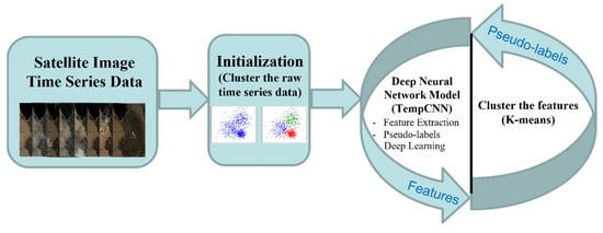
Figure 1.
Overall flow for the proposed method, including the deep neural network model and clustering model.
- We propose a novel unsupervised cluster training framework to cluster the unlabeled SITS data for land cover analysis. The method assigns pseudo-labels to samples to train the feature extractor network, then clusters the generated deep features to get new pseudo-labels. The iteratively pseudo-supervised training improves the ability of the feature extraction network;
- An approach for dealing with large-scale SITS datasets is demonstrated, which handles millions of SITS samples for K-means clustering without the use of pre-trained tasks and prior knowledge;
- The proposed method is portable, and various feature extractor networks and clustering algorithms can be integrated for different SITS clustering tasks. Extensive experiments verify the superiority of our method compared to the state-of-the-art K-means clustering algorithms, particularly on a large-scale dataset.
The rest of this article is organized as follows: Section 2 introduces two SITS datasets and details the proposed algorithm. Section 3 presents evaluation metrics and visual results of the SITS clustering experiments. Section 4 discusses the robustness of the model by using different feature extraction networks and the number of cluster centers. A comparison experiment between a single-temporal image and time-series images, and the prospects of DTIC, will also be mentioned in this section. Finally, Section 5 concludes this paper.
2. Materials and Methods
This section will report two SITS datasets and detail some methods used in this experiment.
2.1. Study Area
To test the effect of our proposed method, we employed two SITS datasets with different sizes, containing more than 15,000 and 1,100,000 pixel samples, respectively.
2.1.1. Reunion Island Dataset
The Reunion Island Dataset is derived from the public dataset provided by the 2017 TiSeLaC Time Series Land Cover Classification Competition, which is released at https://sites.google.com/site/dinoienco/tiselac-time-series-land-cover-classification-challenge (accessed on 1 July 2021). The dataset was collected from 23 2A-level Landsat 8 images (30 m spatial resolution and 16 day temporal resolution) of Reunion Island in 2014, and each image had a size of 2866 × 2633 pixels. For each pixel at each timestamp, 10 features were taken into account: seven surface reflectance bands (Ultra Blue, Blue, Green, Red, NIR, SWIR1, and SWIR2) plus three indices (NDVI, NDWI, and BI). Cloudy observations were filled using pixel-wise multi-temporal linear interpolation on each multi-spectral band (OLI) individually, and complementary radiometric indices were computed. Figure 2 depicts a general overview of the study area. The 2012 Corine Land Cover map and the 2014 farmers’ graphical land parcel registration were used to create reference land cover data. The dataset’s land cover is divided into nine land categories, including cities and towns, artificial surfaces, forests, sparse vegetation, rock bare terrain, grassland, sugarcane, other crops, and water, which covers the majority of Reunion Island’s common surface types. It is well known that imbalanced datasets have a great impact on clustering performance. To assess the performance of different K-means algorithms objectively, we removed four extremely small classes and utilized a dataset that is generally balanced. The detailed class distribution is shown in Table 1.
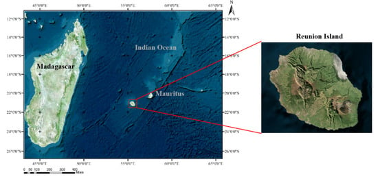
Figure 2.
Overview of the Reunion Island Dataset.

Table 1.
The detailed class distribution on the Reunion Island Dataset.
2.1.2. Imperial Dataset
To test the effect of the proposed method on large-scale and imbalanced datasets, we employed the Imperial Dataset. The Imperial Dataset is made up of 23 cloud-free Landsat 8 land surface reflectance pictures (30 m spatial resolution) taken in Imperial County, CA, USA, between 2016 and 2018. Figure 3 depicts the research area overview. Figure 3 depicts a general overview of the study area. The seven surface reflectance bands (Ultra Blue, Blue, Green, Red, NIR, SWIR1, and SWIR2) of Landsat 8 imaging are presented in each pixel at each timestamp. The real labels refer to the crop mapping results (https://data.cnra.ca.gov/dataset/statewide-crop-mapping (accessed on 19 March 2022)) of California in the United States since 2018, and we selected seven categories with more numbers. Alfalfa, grasses, carrots, onions/garlic, lettuce, citrus, and corn are among the seven land cover classifications represented in this dataset. The detailed class distribution is shown in Table 2.
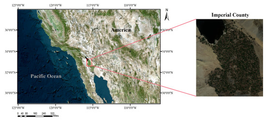
Figure 3.
The overview of the Imperial Dataset.

Table 2.
The detailed class distribution of the Imperial Dataset.
2.2. Deep Temporal Iterative Clustering (DTIC)
This section details our proposed deep temporal iterative clustering (DTIC) method. The DTIC algorithm is an end-to-end unsupervised training clustering algorithm applied to SITS without prior knowledge from specialists and pre-training tasks, which consists of two components: a feature extraction network and a clustering algorithm. First of all, before we train the feature extraction network, we need to initialize the original SITS data to be pseudo-labels. Afterward, we train the feature extraction network using the pseudo-labels, then clustering the generated features using a clustering method such as K-means, and pseudo-supervised training iteratively. We optimize the weight of the feature extraction network and assess the clustering performance in each iteration. The training process is summarized in Algorithm 1.
| Algorithm 1 DTIC |
| Require: The dataset, ; The number of clusters, ; Ensure: The clustering result
|
Most deep clustering algorithms need a pre-training task [32,33,34], while due to the complexity of SITS data, the pre-training tasks are not applicable in this field. We adopt an initialization way to solve this problem. Initialization for clustering in step 1 has been extensively investigated. In DTIC, we use a well-known clustering algorithm, K-means, to get initialized pseudo-labels by clustering original data. For the feature extraction network in step 2, we use TempCNN proposed by [35]. TempCNN is a supervised learning architecture that is inherently designed for time series data. They have been researched for SITS classification and proved their ability to classify time series. The core function of TempCNN is to extract features from multi-spectral remote sensing time series data using 1D convolution along the time series dimension. The receptive field range is determined by the size of the convolution kernel, which can sense fixed time series neighborhood range information for encoding during feature extraction. As shown in Figure 4, at the first stage, time series convolution layers are stacked for feature coding based on time neighborhood, and the remote sensing time series data are coded to the feature coding result with the time series dimension. Each convolution layer is realized by 1D time series convolution, batch normalization, ReLU activation, and Dropout. After that, the encoded feature result is stretched from the 2D to 1D vector, which is used as the final feature to the clustering.
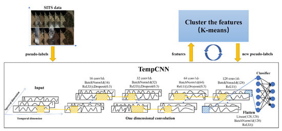
Figure 4.
The overall framework of the proposed algorithm with the TempCNN feature extraction network.
If denoted by , the feature extraction network mapping of TempCNN, where is the set of corresponding parameters. Traditionally, these parameters are learned with supervision, such as each sample of SITS data is paired with a label . When pseudo-supervised deep learning training is performed, we need to assign each sample to a pseudo-label , so we add a layer of linear classifier to the bottom of the network to get the pseudo-labels. The classifier’s parameter and mapping’s parameter are jointly learned by optimizing the following Equation (1), where is multinomial logistic loss. The cost function is minimized by computing the gradient using Adam [36] and back propagation [37].
For clustering in step 4, after using TempCNN in step 3, the features created, the clustering is to split into separate groups using Euclidean distance. For each pixel sample, the feature is a 1 × 128 vector. Specifically, it uses Equation (2) to simultaneously learn a centroid matrix and the cluster assignments of each SITS data . The Equation (1) aims to produce a collection of optimal assignments as well as a centroid matrix . represents the amount of SITS data:
These assignments are then used as pseudo-labels for deep learning; the centroid matrix is not employed.
The existence of trivial solutions is a characteristic of any approach that learns a discriminative classifier and labels simultaneously. To prevent trivial solutions, such as empty cluster, we use the approach in [38]. When a cluster becomes empty during the experiment, we select a non-empty cluster at random and utilize its centroid as the replacement centroid for the empty cluster with a little random perturbation. The points from the non-empty cluster are then reassigned to the two new clusters. To prevent trivial solutions, such as most data assigned to a small number of clusters, then the parameters will discriminate exclusively between those clusters, and the convnets will predict the same result regardless of the input. This problem can be addressed by sampling data based on a fair distribution throughout the classes, or pseudo-labels. Moreover, we also set the maximum and minimum values for each category in the clustering process.
3. Experiments and Results
This section shows the performance metrics and measures the effect of DTIC clustering on two different datasets. The optimized K-means Method Faiss (FAISS) implemented by Facebook AI Laboratory in New York, America [38], K-means in Scikit-learn [39], are both K-means clustering algorithms that are compared with the DTIC method. Due to the sensitivity of the K-means clustering algorithm regarding initial cluster centers, we undertake two groups of experiments for each dataset to demonstrate the efficiency of DTIC under varied initial conditions. One initializes each cluster center by random sample. The other is to initialize each cluster center by the mean vector of each class as the best-case for comparison.
3.1. Evaluation Metrics
To justify the proposed methods, three evaluation approaches are used to measure the quality of clustering results generated by different cluster methods: Clustering Accuracy (ACC) [40], Normalized Mutual Information (NMI) [41], and Adjusted Rand Index (ARI) [42].
- ACC: ACC is a popular metric for assessing clustering outcomes. It is calculated using the acquired clustering assignments and ground truth labels in the following Equation (3):where is the number of samples, represents ground truth labels, represents acquired cluster results, map () is the permutation function that maps obtained cluster labels to their corresponding ground truth labels, and represents a function that equals one if = and zero otherwise.
- NMI: NMI is used to assess the same information shared between two different assignments A and B, defined as:where represents ground truth labels, for cluster results, for mutual information between and , and and for entropy used. The degree of correlation between and is evaluated by NMI. The greater the connection between and , the closer NMI becomes to 1. On the contrary, NMI has 0 value if and are unrelated.
- We use the NMI between the clustering results and the true labels to measure the clustering quality.
- We reassign the data to a new set of clusters for each epoch with no assurance of stability. Measuring the NMI between clusters at epochs t − 1 and t provides insight into the stability of our model.
- ARI: ARI is the version of the Rand Index that takes corrected-for-chance into account. A baseline is set by using the expected similarity of all pairwise comparisons between clustering assignments. Traditionally, the Permutation Model for clustering assignments was used to fix the Rand Index (the number and size of clusters within a clustering are fixed, and all random clustering assignments are generated by shuffling the elements between the fixed clusters). is the number of sample pairs needed to group a total of samples into classes. For a clustering task and cluster assignment , we define as the number of pairs that are in the same clustering in both C and P, and as the number of pairs that are in different clustering assignments in both C and P. The following Equation (5) describes the Rand Index:
However, the permutation model’s premises are routinely violated; in many clustering circumstances, either the number of clusters or their size distribution varies dramatically. Consider that the number of clusters in K-means is determined by the practitioner, but the sizes of those clusters are inferred from the data. Variations in the Adjusted Rand Index cater to various random clustering theories. Although the Rand Index can only provide values between 0 and +1, the Adjusted Rand Index can return negative values if the index is lower than the intended index. Equation (6) explains how to calculate it:
Note that the ground truth label is just used in the analysis of the clustering results and does not participate in any training process of the experiment.
3.2. Implementation Details
For the feature extraction process, we use a TempCNN architecture which consists of four 1D convolutional layers with 16, 32, 64 and 128 filters; first, we use 1D batch normalization to unify scattered data. Second, original feature data is converted by stacking four-layer temporal convolution layers. Each convolution layer is realized by temporal convolution, 1D batch normalization, ReLU activation, and Dropout 0.3. The step size of convolution is set to 1, and the corresponding edge filling of the convolution kernel is set to maintain the integrity of temporal length. Finally, the encoded feature results are stretched from 2D to 1D vectors by a linear layer with an out channel set to 128. For the clustering process, we use the optimized K-means [38]. After the clustering process, we add a linear full connection layer from 128 channels to 5 channels at the bottom of the feature extraction network as a classifier. In the training process, we apply the Adam optimizer [36] and Focal Loss function [43]. The learning rate is set to 0.001, exponential decay rate set to [0.9, 0.999], and batch size is set to 32. We implemented this model using Pytorch and trained it for 300 epochs.
3.3. Results on the Reunion Island Dataset
In this experiment, we train DTIC on the dataset of Reunion Island (15,517 pixel samples distributed into 5 classes). The true label is ignored in the training process and is only used for accurate comparison.
As shown in Figure 5, we observe the dynamic changes in evaluation indexes along training to measure the applicability of the proposed algorithm. Figure 5a shows that the curve of loss function keeps decreasing during the training process. This means that the predicted value of the neural network is nearing the pseudo-labels, and the extracted features are getting more suited for clustering. Figure 5b reveals the evolution of the NMI between the clusters at epochs t − 1 and t during training. We find the curve is rising steadily, which indicates that the reassignments are decreasing and the clusters are becoming more stable. However, NMI tends to 1 but swings slightly, demonstrating that a small proportion of SITS data are regularly reassigned between epochs. Figure 5c depicts the evolution of the NMI, ACC, and ARI between the cluster assignments and the true labels during training. It evaluates the model’s ability to forecast information at the true class level. The growing dependence between clusters and true labels indicates that our features are gradually capturing details about object classes. Unlike supervised learning, our method lacks true labels to determine the training direction, resulting in considerable fluctuations but an overall improvement in accuracy.
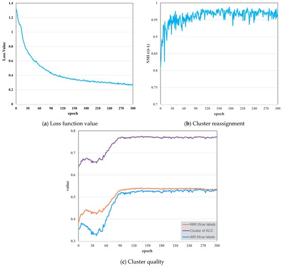
Figure 5.
The preliminary studies of the random initial cluster centers experiment on the Reunion Island Dataset. (a) Loss function; (b) cluster reassignment; (c) cluster quality.
Table 3 exhibits the clustering performance of the Reunion Island Dataset with random initial cluster centers. The proposed clustering algorithm iterates 300 epochs and the best performance is presented. Other K-means clustering methods are repeated 20 times, and 50 random initial center sets are selected each time. In the comparative research, K-means and FAISS cluster the raw features of Reunion Island Dataset and we also present the best results in these experiments. For each pixel sample, the raw feature is a 1 × 230 vector. Table 3 demonstrates that DTIC consistently achieves the best results based on the three criteria, and DTIC wins by a significant margin of 11.4%, 9.7%, and 12.2% over the second-best result for each respective criterion.

Table 3.
A comparison of different methods on Reunion Island Dataset with random initial cluster centers. The bolded results show the best results.
Figure 6 exhibits the number and proportion of different categories by using different algorithms in this experiment. There is a trivial solution in the traditional K-means algorithm, in which only a small percentage of rocks and bare soil (pink) is recognized. This phenomenon does not appear in other optimized K-means methods and DTIC is the most similar to the true quantity proportion.
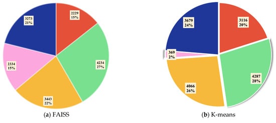
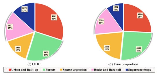
Figure 6.
Quantity and percentage of each class on the Reunion Island Dataset using different methods implemented with random initial cluster centers. (a) FAISS; (b) K-means; (c) DTIC; (d) true proportion.
Figure 7 shows the generated maps using different clustering algorithms and the reference map in visualization, respectively. We find that all methods can roughly identify the correct positions of different categories., particularly in the forest (green). However, the K-means clustering algorithm causes confusion between sparse vegetation (yellow) and water (pink), which leads to a trivial solution. For FAISS and K-means, they both identified a part of urban and built-up (red) in the wrong position. Some sparse vegetation (yellow) and rocks and bare soil (pink) are identified as urban and built-up (red) by all methods. These issues are also present in the clustering map generated by DTIC, while they are mitigated to acceptable degrees.
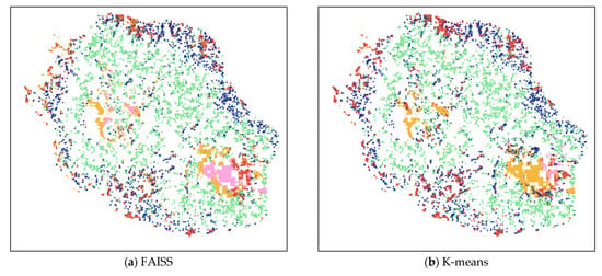
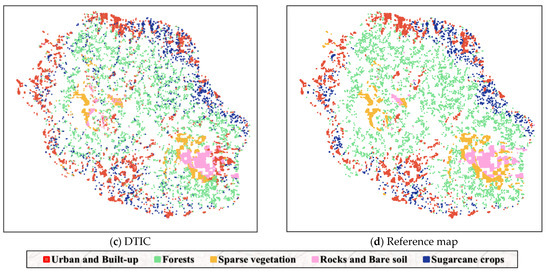
Figure 7.
Clustering maps of the Reunion Island Dataset produced using different methods with random initial cluster centers. (a) FAISS; (b) K-means; (c) DTIC; (d) reference map.
Since the K-means algorithm is susceptible to the initial clustering center, we use a set of excellent initial clustering centers to eliminate this influence. Concretely, this experiment employs the average of each class’s time series feature as initial cluster centers using a seed clustering method. Technically, this experiment is semi-supervised because it starts with labeled samples. The preliminary studies of averaged initial cluster center experiment are shown as Figure 8. We adopt the same model structure as the random initial cluster centers experiment and iterate it for 300 epochs. Figure 8 depicts the evolution of several assessment indices throughout the training process. In the training process, the network will proceed in the right direction because the initial clustering centers are defined. Compared with the random initial centers experiment, the fluctuation of training results significantly decreased. In addition, the curve stabilizes quickly and the accuracy of DTIC is higher, around 10%, than that of the random initial centers experiment since the semi-supervision training is better than the unsupervised.
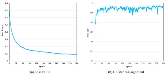
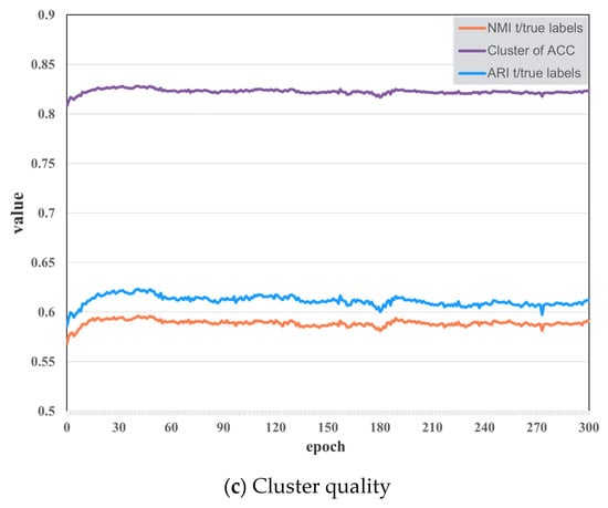
Figure 8.
The preliminary studies of the averaged initial cluster centers experiment on the Reunion Island Dataset. (a) Loss function; (b) cluster reassignment; (c) cluster quality.
Table 4 illustrates the clustering performance of all methods when the average time series features of the true-labels set are utilized for initialization. DTIC uses the published labels of the testing set and it is only utilized to create initial cluster centers in this experiment. The other methods are repeated 50 times to select the optimal performance and cluster the raw features. The performance is assessed using the three criteria listed in Section 3.1. Table 4 demonstrates that DTIC consistently achieves the best results, with a significant victory margin of 22.0%, 17.4%, and 21.3% over the second-best result for each criterion, respectively. The other methods have similar accuracy, which indicates that the two methods are not optimized from the structure. Moreover, the two experimental precisions of FAISS are the same, which means this algorithm is relatively mature for determining the initial cluster centers of K-means. On the contrary, DTIC adds a lot of uncertain factors by combining deep training into clustering, resulting in a significant improvement in this experiment. To summarize, the accuracy of clustering is higher than that of random initial centers due to assigning the cluster center with a semi-supervised approach. Each criterion of the DTIC is significantly greater than that of other methods. When the cluster center is specified, the generated results using DTIC are promising.

Table 4.
A comparison of different methods on the Reunion Island Dataset with averaged initial cluster centers. The bolded results show the best results.
Figure 9 exhibits the number and proportion of different classes by using different methods with averaged initial cluster centers. Due to the specified center point, we find the trivial solution does not appear in this experiment. The clustering assignment of all methods is significantly better than that of the random initial cluster centers experiment, and the DTIC method is closest to reality. Nevertheless, other methods recognize a lot more sugarcane crops (blue) than the real situation, but urban and built-up (red) are recognized a little less. This phenomenon illustrates that other methods are not well-suited to the situation where large differences exist in the number of categories. The proposed method eliminates this phenomenon by combining deep training with clustering.
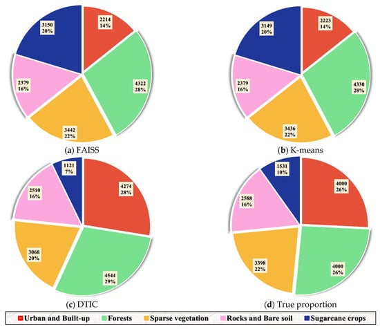
Figure 9.
Quantity and percentage of each class on the Reunion Island Dataset using different methods implemented with averaged initial cluster centers. (a) FAISS; (b) K-means; (c) DTIC; (d) true proportion.
Visually, Figure 10 depicts the clustering map generated by several methods with averaged initial cluster centers and the reference map. As observed, all clustering models detect position information more precisely than the random initial centers experiment. Although some urban and built-up (red) positions are identified as sugarcane crops (blue) by FAISS and K-means methods, DTIC eliminates this phenomenon and achieves the best results.
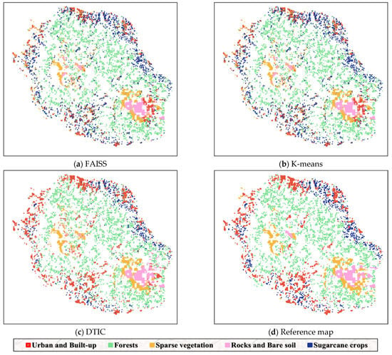
Figure 10.
Clustering maps of the Reunion Island Dataset produced by using different methods with averaged initial cluster centers. (a) FAISS; (b) K-means; (c) DTIC; (d) reference map.
3.4. Results on the Imperial Dataset
Additionally, we conduct experiments on the Imperial Dataset (1,147,604 pixel samples distributed into 7 classes) to evaluate the performance on a large-scale uneven dataset. The raw characteristics are similar in both datasets; however, it adopts principal component analysis (PCA) to solve extracted features compared to the above model. In addition, the model adopts the same structure as the previous experiment.
We only iterate 150 epochs to get the results because of the vast amount of data. Other K-means clustering methods are completed 20 times with 50 sets of random cluster centers each time. In the comparative research, K-means and FAISS cluster the raw features of the Imperial Dataset and the raw feature of each pixel sample is a 1 161 vector. The best performance of all methods on the Imperial Dataset is illustrated in Table 5. It can be seen that DTIC outperforms the other alternatives by 11.4%, 9.7%, and 12.2%, respectively, on each criterium. The accuracy of FAISS and K-means methods is only around 30%. This demonstrates that other methods are not well-suited to large-scale and imbalanced datasets. Meanwhile, the DTIC obtained a 60% accuracy on this dataset, indicating that the proposed method still applies to large-scale and imbalanced datasets.

Table 5.
A comparison of different methods on the Imperial Dataset with random initial cluster centers. The bolded results show the best results.
Figure 11 exhibits the number and proportion of different categories by using different algorithms on the Imperial Dataset. The number of categories in FAISS and K-means are quite similar, while they are obviously different from the truth. This phenomenon also shows that the two models both fail to cluster the large-scale and imbalanced dataset. Although the DTIC method is generally different from the actual situation, it identifies the number differences between categories. For instance, the alfalfa (pink) accounts for a large proportion of the clustering assignments, which is consistent with the reference map. Correspondingly, the DTIC method can identify the differences between various quantity categories well by connecting clustering and deep training.
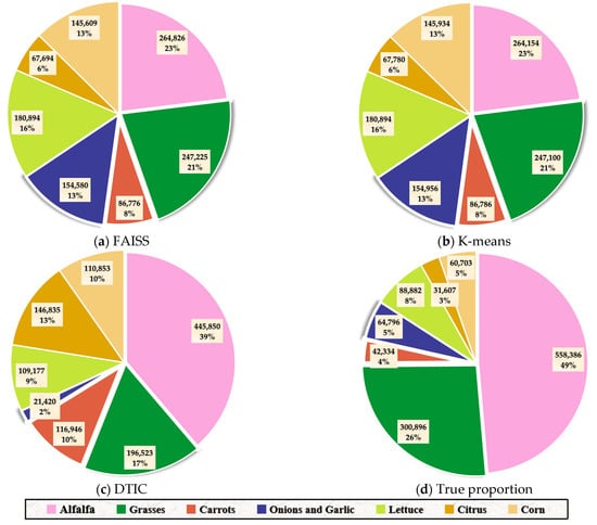
Figure 11.
Quantity and percentage of each class on the Imperial Dataset using different methods implemented with random initial cluster centers. (a) FAISS; (b) K-means; (c) DTIC; (d) true proportion.
Figure 12 shows the generated maps using different methods and the reference map of the Imperial Dataset visualization, respectively. The clustering maps of the FAISS and K-means are similar, while they are completely different from the reference map. Although the DTIC method generally identifies the true position information of several classes, some alfalfa (pink) and grasses (dark green) are identified as citrus (orange) in the lower right corner of map and onions and garlic (blue) are not identified; in general, the clustering effect of DTIC is acceptable.
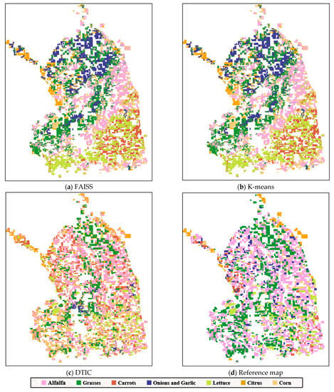
Figure 12.
Clustering maps of the Imperial Dataset produced using different methods with random initial cluster centers. (a) FAISS; (b) K-means; (c) DTIC; (d) reference map.
Table 6 displays the clustering performance of different methods when the averaged initial cluster centers are specified. The three criteria are also applied to performance evaluation. It can be concluded that DTIC outperforms the other methods by 56.7%, 57.7%, and 73.9% relative to the second-best results on each criterion, respectively. We observe that even if the initial clustering center is specified, other methods do not produce an acceptable result. This phenomenon shows that other methods have failed to cluster the large-scale and imbalanced dataset under any initial cluster center conditions. Nevertheless, DTIC has the best performance compared to the Reunion Island Dataset. We consider the qualities of original features and PCA to play an important role in the generated results.

Table 6.
A comparison of different methods on the Imperial Dataset with averaged initial cluster centers. The bolded results show the best results.
Using different clustering methods with averaged initial cluster centers, the number and proportion of distinct categories on the Imperial Dataset are shown in Figure 13. Even if the center points are specified, the clustering assignments of FAISS and K-means are both even. This phenomenon is inconsistent with the real situation, which leads to the failure of two methods. The DTIC method shows the most similar situation to the actual quantity distribution, in which there is a huge difference in quantity between different categories. Owing to the integration of deep training, DTIC successfully identified the quantity difference information between categories and achieved excellent results.
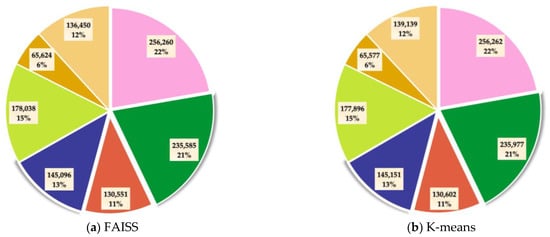
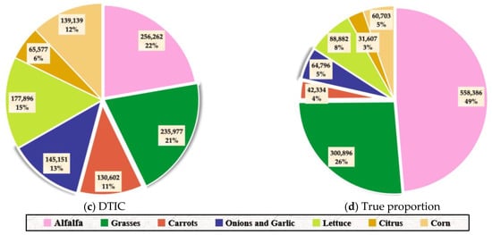
Figure 13.
Quantity and percentage of each class on the Imperial Dataset using different methods implemented with averaged initial cluster centers. (a) FAISS; (b) K-means; (c) DTIC; (d) true proportion.
Clustering maps generated by various methods with averaged initial cluster centers and a reference map of the Imperial Dataset are depicted in Figure 14. It can be seen that the maps of FAISS and K-means are the same as that of the random initial cluster centers experiment, which proves that despite the cluster centers being specified, the two methods cannot identify the correct position at all. Instead, DTIC integrates deep training into clustering and enhances the ability of the model to identify the correct distribution information. When the cluster centers are designated, DTIC identifies more accurate location information, even almost entirely consistent with the reference map. The above phenomenon shows that our method can still achieve good results on a large-scale and imbalanced dataset, especially specifying the initial cluster centers in a seed clustering method.
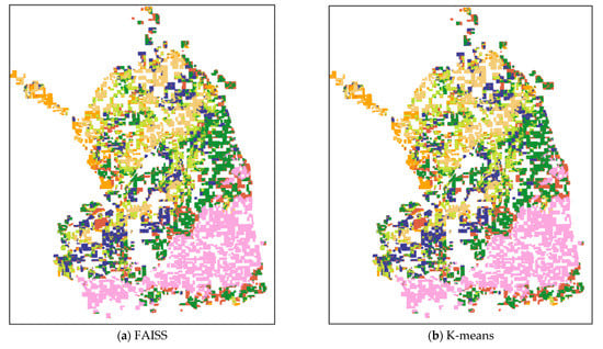
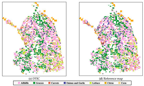
Figure 14.
Clustering maps of the Imperial Dataset were produced using different methods with averaged initial cluster centers. (a) FAISS; (b) K-means; (c) DTIC; (d) reference map.
4. Discussions
The current benchmark for assessing the clustering approach employs a TempCNN architecture trained on two different datasets. To quantify the many biases provoked by this pipeline on DTIC, we examined different quantity cluster centers and a different feature extraction network architecture. Moreover, we conducted a new comparison experiment between a single-temporal image and time-series images and finally proposed the prospects of DTIC.
4.1. Given the Number of Clusters
In this section, we measure the effect of different numbers of cluster centers on clustering performance. A similar downstream task with random initial clusters is presented on the Reunion Island Dataset. This research only modifies on a logarithmic scale and shows the results after 300 epochs in Figure 15. The performance after the same number of epochs for different may not be directly comparable, but it exhibits the hyper-parameter selection utilized in this work. It can be seen that the optimal performance is achieved when is set to 6. Provided that we train our model on this dataset, one would anticipate that is set to 5 to get an acceptable result, but it appears that some argumentation is advantageous. The presence of mixed pixels in remote sensing could explain this phenomenon.
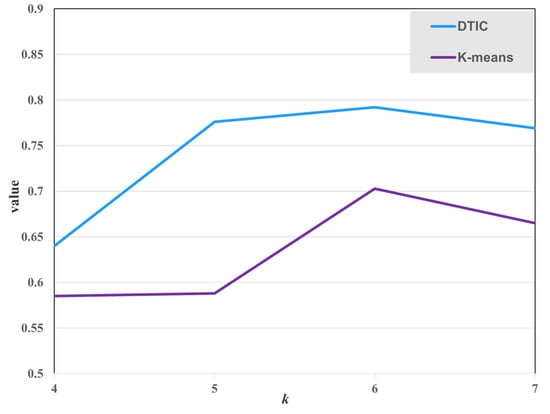
Figure 15.
The clustering performance for various choices of with random initial cluster centers on the Reunion Island Dataset.
4.2. TempCNN vs. LSTM
In a supervised environment, TempCNN and LSTM are equally suited for processing time series sequential data. This experiment evaluates the robustness of DTIC by comparing different feature extraction networks. Table 7 contrasts an LSTM and a TempCNN feature extraction network on the Reunion Island Dataset by using DTIC. We also report the results of FAISS [38] for a controlled experiment. Regardless of the approach, a deep clustering architecture improves the performance of the objective task significantly. Similar to supervised learning, we find that the TempCNN structure outperforms the LSTM structure in DTIC, which demonstrates that the difference between supervised stays comparable for DTIC architectures.

Table 7.
A comparison of the optimal performance of various K-means clustering algorithms on the Reunion Island Dataset with random and averaged initial cluster centers.
4.3. Single-Temporal Image vs. Multi-Temporal Images
To illustrate the advantages of using time-series images, we conducted a new comparison experiment between a single-temporal image and time-series images of the Reunion Island Dataset in an unsupervised way. Single-temporal images were taken on the 188th day of 2014, when crops were growing vigorously. For clustering the single-temporal image, the raw features are input to two methods. The clustering accuracy of the comparison experiment is shown as Table 8. It can be seen that the performance of using time-series images is significantly better than that of using single-temporal image. This result proves that using satellite image time series data causes a great improvement in land cover analysis. Owing to the use of depth features, the clustering accuracy of DTIC is higher than the other clustering method in both situations.

Table 8.
The clustering accuracy of the comparison experiment between a single-temporal image and multi-temporal images on the Reunion Island Dataset.
4.4. Prospects of DTIC
While DTIC offers accuracy benefits, its computing efficiency has tremendous potential for improvement. For different datasets, DTIC models with defined initial cluster centers outperform those with random centers since semi-supervised training is theoretically preferable to entirely unsupervised training. However, the accuracy of FAISS is nearly equal regardless of whether the initial cluster centers are specified, indicating that this method is relatively good for determining the cluster centers. This is also the direction for improving the DTIC model in the case of completely unsupervised training. Concretely, it is necessary to develop a better method for identifying the cluster centers in a DTIC model so that its accuracy progressively approaches the semi-supervised results. Furthermore, we exclusively provide a novel ideal scenario for clustering large-scale and imbalanced SITS datasets and obtain a promising result. The corresponding network structure and hyper-parameter selection should be changed for the specific land cover analysis task of different SITS datasets. Moreover, we only consider the temporal dimension of each pixel sample in this research. Other dimensions, such as spatial or spectral, are not taken into account. For the feature extraction network, the dimension of the convolution kernel is set to 1, and the depth features are only generated from the temporal dimension of each pixel image. In future research, it is worth trying to combine the time dimension with other dimensions to analyze SITS data.
When the datasets are extremely imbalanced or have an extreme quantity in a category, the accuracy of the initial training is very high, but the fluctuation is large or the accuracy continues to decline. Ultimately, the value of the random seed has a significant influence on the results through experiments. We employ 35 and 50 random seeds for the two datasets in this study, respectively. If the random seed is not appropriate, the training accuracy will continue to decline and produce undesirable results, which is also the place where the follow-up work can be enhanced: finding a strategy to make the training progress towards correct orientation under arbitrary random seeds.
5. Conclusions
In this paper, we proposed DTIC, a scalable clustering approach inspired by the classic deep cluster framework [31], for the unsupervised learning of SITS data. It alternates between clustering the features produced by the neural network and updating the weights of network by using pseudo-labels in a discriminative loss. To demonstrate the effects of DTIC, we conducted clustering studies on two SITS datasets. DTIC outperformed other methods in three criteria and achieved the best performance in all experiments. The proposed method makes few assumptions about the inputs and requires no pre-training tasks, making it a strong choice for learning deep representations to cluster SITS data that lack annotations. Furthermore, we exclusively provided a novel approach and idea for clustering large-scale and imbalanced datasets and obtained promising results. The corresponding network structure and hyper-parameter selection depend on the specific tasks. Departing from the other K-means methods, our proposed method is still applicable in the case of poor data quality.
Author Contributions
Conceptualization, W.G. and S.G.; methodology, W.G. and P.T.; software, W.G. and W.Z.; data curation, W.Z. and Z.Z.; writing—original draft preparation, W.G.; writing—review and editing, Z.Z. and P.T.; visualization, W.G. and W.Z.; supervision, Z.Z. and S.G. All authors have read and agreed to the published version of the manuscript.
Funding
This research was funded by the National Natural Science Foundation of China (Grant No. 12001504) and the Youth Innovation Promotion Association, CAS (No. 2022127).
Data Availability Statement
Not applicable.
Acknowledgments
We would like to thank Dino Ienco and Raffaele Gaetano for releasing the TiSeLaC (Time Series Land Cover Classification Challenge) Reunion Island Dataset.
Conflicts of Interest
The authors declare no conflict of interest.
References
- Ma, L.; Liu, Y.; Zhang, X.; Ye, Y.; Yin, G.; Johnson, B.A. Deep learning in remote sensing applications: A meta-analysis and review. ISPRS J. Photogramm. Remote Sens. 2019, 152, 166–177. [Google Scholar] [CrossRef]
- Navalgund, R.R.; Jayaraman, V.; Roy, P.S. Remote sensing applications: An overview. Curr. Sci. 2007, 93, 1747–1766. [Google Scholar]
- Justice, C.O.; Townshend, J.; Vermote, E.F.; Masuoka, E.; Wolfe, R.E.; Saleous, N.; Roy, D.P.; Morisette, J.T. An overview of MODIS Land data processing and product status. Remote Sens. Environ. 2002, 83, 3–15. [Google Scholar] [CrossRef]
- Drusch, M.; Del Bello, U.; Carlier, S.; Colin, O.; Fernandez, V.; Gascon, F.; Hoersch, B.; Isola, C.; Laberinti, P.; Martimort, P. Sentinel-2: ESA’s optical high-resolution mission for GMES operational services. Remote Sens. Environ. 2012, 120, 25–36. [Google Scholar] [CrossRef]
- Feng, L.; Li, J.; Gong, W.; Zhao, X.; Chen, X.; Pang, X. Radiometric cross-calibration of Gaofen-1 WFV cameras using Landsat-8 OLI images: A solution for large view angle associated problems. Remote Sens. Environ. 2016, 174, 56–68. [Google Scholar] [CrossRef]
- Li, Z.; Shen, H.; Li, H.; Xia, G.; Gamba, P.; Zhang, L. Multi-feature combined cloud and cloud shadow detection in GaoFen-1 wide field of view imagery. Remote Sens. Environ. 2017, 191, 342–358. [Google Scholar] [CrossRef] [Green Version]
- Jönsson, P.; Eklundh, L. TIMESAT—A program for analyzing time-series of satellite sensor data. Comput. Geosci. 2004, 30, 833–845. [Google Scholar] [CrossRef] [Green Version]
- Sagawa, T.; Yamashita, Y.; Okumura, T.; Yamanokuchi, T. Satellite derived bathymetry using machine learning and multi-temporal satellite images. Remote Sens. 2019, 11, 1155. [Google Scholar] [CrossRef] [Green Version]
- Ienco, D.; Interdonato, R.; Gaetano, R.; Minh, D.T. Combining Sentinel-1 and Sentinel-2 satellite image time series for land cover mapping via a multi-source deep learning architecture. ISPRS J. Photogramm. Remote Sens. 2019, 158, 11–22. [Google Scholar] [CrossRef]
- Ndikumana, E.; Ho Tong Minh, D.; Baghdadi, N.; Courault, D.; Hossard, L. Deep recurrent neural network for agricultural classification using multitemporal SAR Sentinel-1 for Camargue, France. Remote Sens. 2018, 10, 1217. [Google Scholar] [CrossRef] [Green Version]
- Cai, Y.; Guan, K.; Peng, J.; Wang, S.; Seifert, C.; Wardlow, B.; Li, Z. A high-performance and in-season classification system of field-level crop types using time-series Landsat data and a machine learning approach. Remote Sens. Environ. 2018, 210, 35–47. [Google Scholar] [CrossRef]
- Moskolaï, W.R.; Abdou, W.; Dipanda, A. Application of deep learning architectures for satellite image time series prediction: A review. Remote Sens. 2021, 13, 4822. [Google Scholar] [CrossRef]
- Pekel, J.; Cottam, A.; Gorelick, N.; Belward, A.S. High-resolution mapping of global surface water and its long-term changes. Nature 2016, 540, 418–422. [Google Scholar] [CrossRef]
- Inglada, J.; Vincent, A.; Arias, M.; Marais-Sicre, C. Improved early crop type identification by joint use of high temporal resolution SAR and optical image time series. Remote Sens. 2016, 8, 362. [Google Scholar] [CrossRef] [Green Version]
- Khiali, L.; Ndiath, M.; Alleaume, S.; Ienco, D.; Ose, K.; Teisseire, M. Detection of spatio-temporal evolutions on multi-annual satellite image time series: A clustering based approach. Int. J. Appl. Earth Obs. Geoinf. 2019, 74, 103–119. [Google Scholar] [CrossRef]
- Liu, J.; Xue, Y.; Ren, K.; Song, J.; Windmill, C.; Merritt, P. High-performance time-series quantitative retrieval from satellite images on a GPU cluster. IEEE J. Sel. Top. Appl. Earth Obs. Remote Sens. 2019, 12, 2810–2821. [Google Scholar] [CrossRef] [Green Version]
- Gonçalves, R.; Zullo, J.; Amaral, B.D.; Coltri, P.P.; Sousa, E.D.; Romani, L.S. Land use temporal analysis through clustering techniques on satellite image time series. In Proceedings of the 2014 IEEE Geoscience and Remote Sensing Symposium, Quebec City, QC, Canada, 13–18 July 2014; IEEE: Piscataway, NJ, USA, 2014; pp. 2173–2176. [Google Scholar]
- Fränti, P.; Rezaei, M.; Zhao, Q. Centroid index: Cluster level similarity measure. Pattern Recognit. 2014, 47, 3034–3045. [Google Scholar] [CrossRef]
- Nguyen, D.T.; Chen, L.; Chan, C.K. Clustering with multiviewpoint-based similarity measure. IEEE Trans. Knowl. Data Eng. 2011, 24, 988–1001. [Google Scholar] [CrossRef]
- Dash, M.; Liu, H. Feature selection for clustering. In Proceedings of the Pacific-Asia Conference on Knowledge Discovery and Data Mining, Maebashi City, Japan, 9–12 December 2002; Springer: Berlin/Heidelberg, Germany, 2000; pp. 110–121. [Google Scholar]
- Krishna, K.; Murty, M.N. Genetic K-means algorithm. IEEE Trans. Syst. Man Cybern. Part B (Cybern.) 1999, 29, 433–439. [Google Scholar] [CrossRef] [PubMed] [Green Version]
- Zhang, Z.; Tang, P.; Duan, R. Dynamic time warping under pointwise shape context. Inf. Sci. 2015, 315, 88–101. [Google Scholar] [CrossRef]
- Zhou, S.; Xu, H.; Zheng, Z.; Chen, J.; Bu, J.; Wu, J.; Wang, X.; Zhu, W.; Ester, M. A Comprehensive Survey on Deep Clustering: Taxonomy, Challenges, and Future Directions. arXiv 2022, arXiv:2206.07579. [Google Scholar]
- Alturki, A.; Bchir, O.; Ismail, M.B. Joint Deep Clustering: Classification and Review. Int. J. Adv. Comput. Sci. Appl. 2021, 12, 863–874. [Google Scholar] [CrossRef]
- Aljalbout, E.; Golkov, V.; Siddiqui, Y.; Strobel, M.; Cremers, D. Clustering with deep learning: Taxonomy and new methods. arXiv 2018, arXiv:1801.07648. [Google Scholar]
- Alqahtani, A.; Ali, M.; Xie, X.; Jones, M.W. Deep Time-Series clustering: A review. Electronics 2021, 10, 3001. [Google Scholar] [CrossRef]
- Tian, F.; Gao, B.; Cui, Q.; Chen, E.; Liu, T. Learning deep representations for graph clustering. In Proceedings of the AAAI Conference on Artificial Intelligence, Québec City, QC, Canada, 27–31 July 2014; Volume 28. [Google Scholar]
- Li, F.; Qiao, H.; Zhang, B. Discriminatively boosted image clustering with fully convolutional auto-encoders. Pattern Recognit. 2018, 83, 161–173. [Google Scholar] [CrossRef] [Green Version]
- Song, C.; Liu, F.; Huang, Y.; Wang, L.; Tan, T. Auto-encoder based data clustering. In Proceedings of the Iberoamerican Congress on Pattern Recognition, Havana, Cuba, 20–23 November 2013; Springer: Berlin/Heidelberg, Germany, 2013; pp. 117–124. [Google Scholar]
- Alqahtani, A.; Xie, X.; Deng, J.; Jones, M.W. A deep convolutional auto-encoder with embedded clustering. In Proceedings of the 2018 25th IEEE International Conference on Image Processing (ICIP), Athens, Greece, 7–10 October 2018; IEEE: Piscataway, NJ, USA, 2018; pp. 4058–4062. [Google Scholar]
- Caron, M.; Bojanowski, P.; Joulin, A.; Douze, M. Deep clustering for unsupervised learning of visual features. In Proceedings of the European Conference on Computer Vision (ECCV), Munich, Germany, 8–14 September 2018; pp. 132–149. [Google Scholar]
- Lafabregue, B.; Weber, J.; Gançarski, P.; Forestier, G. Deep constrained clustering applied to satellite image time series. In Proceedings of the ECML/PKDD Workshop on Machine Learning for Earth Observation Data (MACLEAN), Würzburg, Germany, 16–20 September 2019. [Google Scholar]
- Chazan, S.E.; Gannot, S.; Goldberger, J. Deep clustering based on a mixture of autoencoders. In Proceedings of the 2019 IEEE 29th International Workshop on Machine Learning for Signal Processing (MLSP), Pittsburgh, PA, USA, 13–16 October 2019; IEEE: Piscataway, NJ, USA, 2019; pp. 1–6. [Google Scholar]
- Gargees, R.S.; Scott, G.J. Deep feature clustering for remote sensing imagery land cover analysis. IEEE Geosci. Remote Sens. Lett. 2019, 17, 1386–1390. [Google Scholar] [CrossRef]
- Pelletier, C.; Webb, G.I.; Petitjean, F. Temporal convolutional neural network for the classification of satellite image time series. Remote Sens. 2019, 11, 523. [Google Scholar] [CrossRef] [Green Version]
- Kingma, D.P.; Ba, J. Adam: A method for stochastic optimization. arXiv 2014, arXiv:1412.6980. [Google Scholar]
- Hecht-Nielsen, R. Theory of the backpropagation neural network. In Neural Networks for Perception; Elsevier: Amsterdam, The Netherlands, 1992; pp. 65–93. [Google Scholar]
- Johnson, J.; Douze, M.; Jégou, H. Billion-scale similarity search with gpus. IEEE Trans. Big Data 2019, 7, 535–547. [Google Scholar] [CrossRef] [Green Version]
- Pedregosa, F.; Varoquaux, G.; Gramfort, A.; Michel, V.; Thirion, B.; Grisel, O.; Blondel, M.; Prettenhofer, P.; Weiss, R.; Dubourg, V. Scikit-learn: Machine learning in Python. J. Mach. Learn. Res. 2011, 12, 2825–2830. [Google Scholar]
- Wu, M.; Schölkopf, B. A local learning approach for clustering. In Advances in Neural Information Processing Systems; MIT Press: Cambridge, MA, USA, 2006; p. 19. [Google Scholar]
- Estévez, P.A.; Tesmer, M.; Perez, C.A.; Zurada, J.M. Normalized mutual information feature selection. IEEE Trans. Neural Netw. 2009, 20, 189–201. [Google Scholar] [CrossRef] [PubMed] [Green Version]
- Steinley, D. Properties of the hubert-arable adjusted rand index. Psychol. Methods 2004, 9, 386. [Google Scholar] [CrossRef] [PubMed]
- Lin, T.; Goyal, P.; Girshick, R.; He, K.; Dollár, P. Focal loss for dense object detection. In Proceedings of the IEEE International Conference on Computer Vision, Venice, Italy, 22–29 October 2017; pp. 2980–2988. [Google Scholar]
Publisher’s Note: MDPI stays neutral with regard to jurisdictional claims in published maps and institutional affiliations. |
© 2022 by the authors. Licensee MDPI, Basel, Switzerland. This article is an open access article distributed under the terms and conditions of the Creative Commons Attribution (CC BY) license (https://creativecommons.org/licenses/by/4.0/).