1. Introduction
With the continuous development of global navigation satellite systems (GNSSs), spaceborne GNSS reflectometry (GNSS-R) technology has become a hot research direction in the field of remote sensing. In 1993, Martín-Neira proposed the concept of the Passive Reflectometry and Interferometry System (PARIS) and the use of GNSS-R for ocean altimetry [
1]. Since then, GNSS-R has been utilized for a range of ocean and land applications, including sea surface altimetry [
2], sea surface wind speed measurements [
3], sea ice detection [
4], and soil moisture measurements [
5]. Over the past few decades, a number of ground-based GNSS-R experiments have been conducted. Many airborne experiments have also been conducted to investigate this new remote sensing technology. Notwithstanding some technological challenges, satellite-based GNSS-R technology has the advantages of low cost and great coverage in some applications [
6]. Currently, there are more than 14 satellites in operation carrying a GNSS-R payload.
UK-DMC (United Kingdom—Disaster Monitoring Constellation), the first satellite carrying a GNSS-R receiver, was launched on 27 September 2003; data from this system have been used to sense ocean roughness. UK TDS-1 (TechDemoSat-1), the second GNSS-R satellite, was launched on the 8 July 2014. On the 15 December 2016, NASA launched eight microsatellites to form the cyclone GNSS (CYGNSS) constellation with the initial objective of monitoring hurricane intensity [
7,
8]. Both TDS-1 and CYGNSS have generated a large amount of data which can be downloaded for scientific research [
9]. On the 5 June 2019, the BuFeng-1 A/B twin satellites, developed by CASTC (China Aviation Smart Technology Co., Shenzhen, China), were launched from the Yellow Sea. One focus of the satellite mission is on the sensing of sea surface wind velocities, and especially typhoons, using GNSS-R [
10].
Sea surface wind speed is an important and commonly used ocean geophysical parameter [
11]. The stability of the wind field plays an important role in ocean circulation and global climate [
12,
13]. Traditional sea surface wind field monitoring methods generally use buoys or coastal meteorological stations, but these methods can only cover small areas with low spatial resolution and expensive equipment [
14]. Microwave scatter meters and synthetic aperture radars can also monitor the global sea surface wind field [
15,
16]. Compared with these traditional wind measurement methods, spaceborne GNSS-R has several advantages, such as rich signal sources and all-weather, all-day, low cost, and large coverage [
17,
18].
GNSS-R technology is basically mature in retrieving sea surface wind speeds. Zavorotny and Voronovich proposed the scattering model theory in 2000 [
19], which can simulate different waveforms of GNSS reflection signals, thus inverting sea surface wind speeds by delayed waveform matching methods [
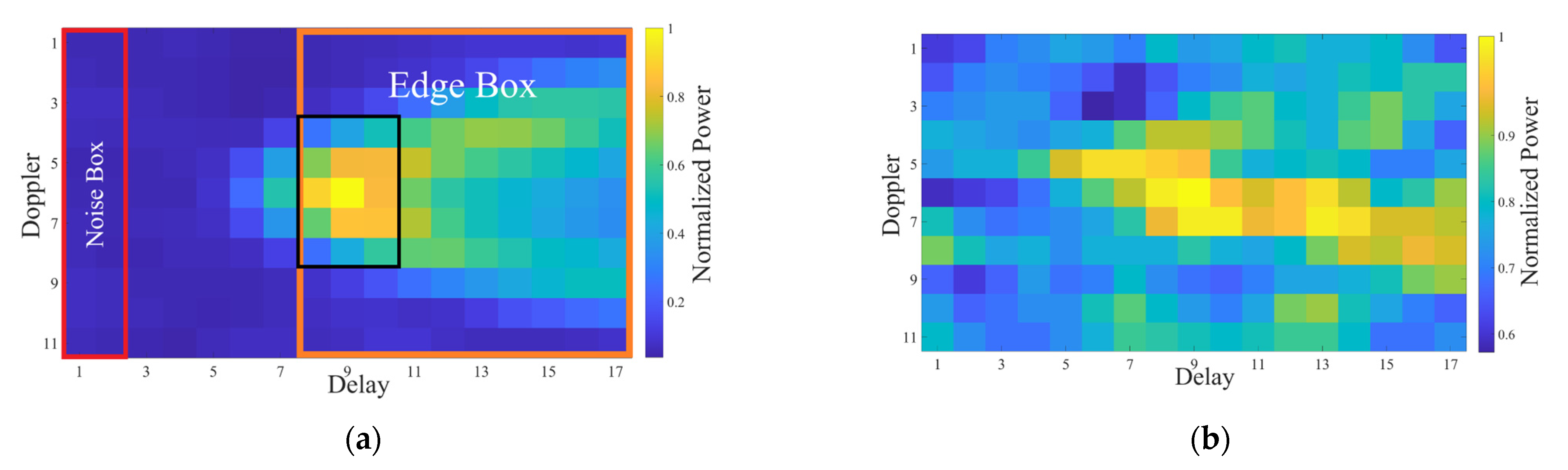
20]. Since then, observations extracted from DDMs (Delay Doppler Maps) have been widely used. DDM is the basic observation data of airborne and spaceborne GNSS-R receivers [
21]. Some DDM observations, such as DDM average (DDMA), are directly related to sea surface roughness [
21]. Other DDM observations can be used as variables for retrieving sea surface parameters. The normalized bistatic radar cross-section (NBRCS), leading edge slope (LES) and signal-to-noise ratio (SNR) have good correlations with the mean square slope (MSS) of the sea surface. Generally, the MSS is mainly affected by the sea surface wind speed [
22].
In recent years, many spaceborne GNSS-R wind speed retrieval models have been developed. Jing et al. demonstrated the effectiveness of NBRCS by proposing some geophysical model functions (GMFs) related thereto [
10]. Bu et al. proposed double- and triple-parameter GMFs with higher retrieval accuracy [
14]. Machine learning methods have also been used to improve the performance of spaceborne GNSS-R wind speed retrieval. Liu Y. et al. proposed a machine learning algorithm based on a multi-hidden layer neural network. The accuracy of their models was significantly higher than that of GMFs [
23]. Many subsequent studies have adopted similar algorithms and obtained results with RMSE of about 1.5–2.0 [
24,
25,
26]. However, most of the above studies observed that it is difficult to use their algorithms to accurately retrieve high sea surface wind speeds [
27,
28]. A few studies have tried to enhance the ability of GNSS-R to retrieve high wind speeds. For instance, Zhang et al. developed machine learning-based models to retrieve wind speeds (20–30 m/s) with an RMSE of 2.64 and a correlation coefficient of 0.25 [
29].
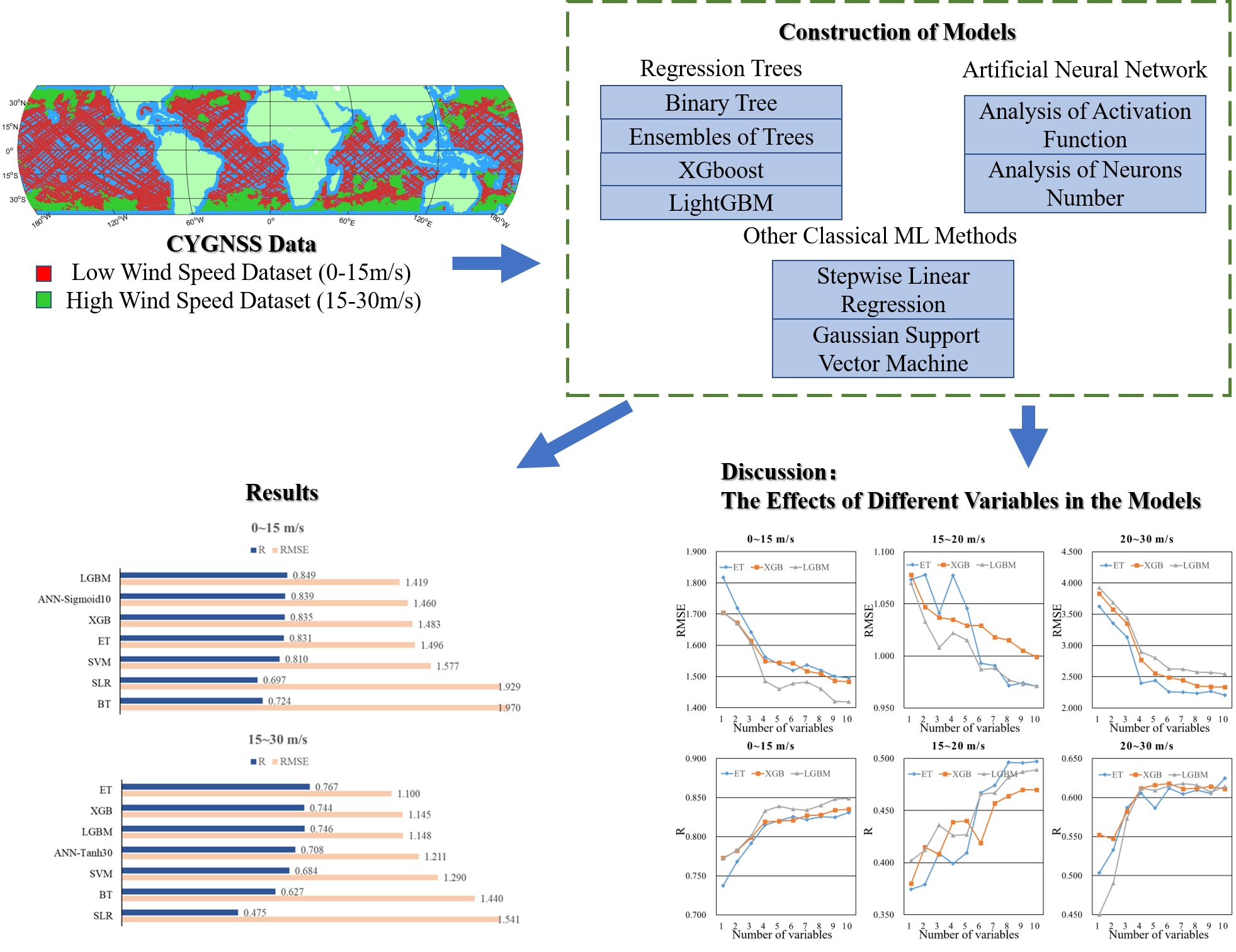
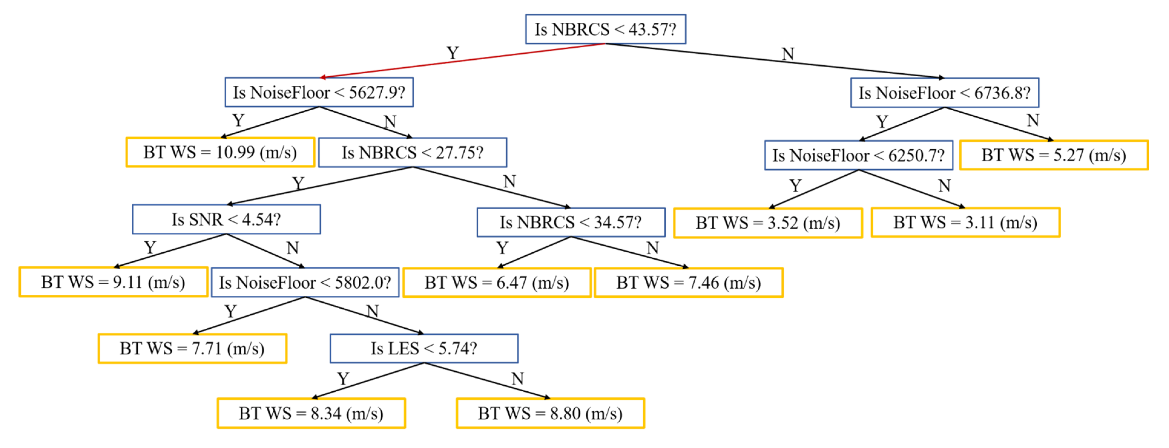
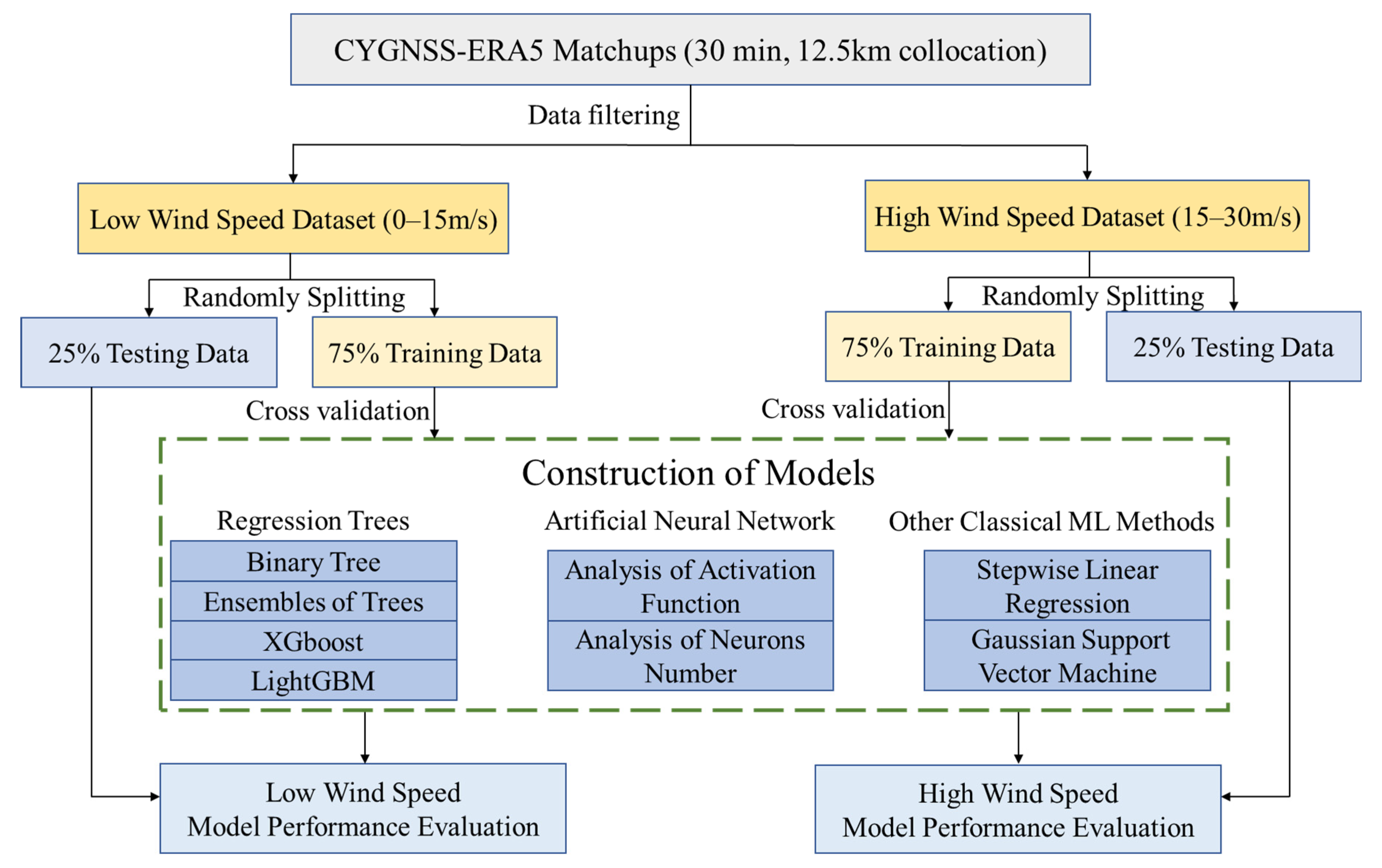
With high wind speed intervals, the Spaceborne GNSS-R data present different distributions and physical characteristics compared to when low wind speed intervals are applied, which leads to the inconsistent performance of different machine learning models. Therefore, this study analyzes the performance of various machine learning models in different wind speed intervals using the following methods: Regression trees (Binary Tree (BT), Ensembles of Trees (ET), XGBoost (XGB), LightGBM (LGBM) ), ANN (Artificial neural network), Stepwise Linear Regression (SLR), and Gaussian Support Vector Machine (GSVM). In this research, the selection of the input parameters for machine learning methods was significant. In this article, a range of variables are considered and evaluated, which are directly or indirectly relevant to sea surface wind speed. The main contributions of the article are as follows:
- (1)
Seven machine learning methods are used to retrieve sea surface wind speed, and their performance is evaluated under two different wind speed ranges.
- (2)
A ranking of the effects of 10 variables on wind speed retrieval is obtained by comparing the performance of different combinations of the variables. This provides a useful guide for variable selection when considering both complexity and accuracy.
- (3)
A filtering algorithm is proposed to process DDM data, achieving both low complexity and good performance.
- (4)
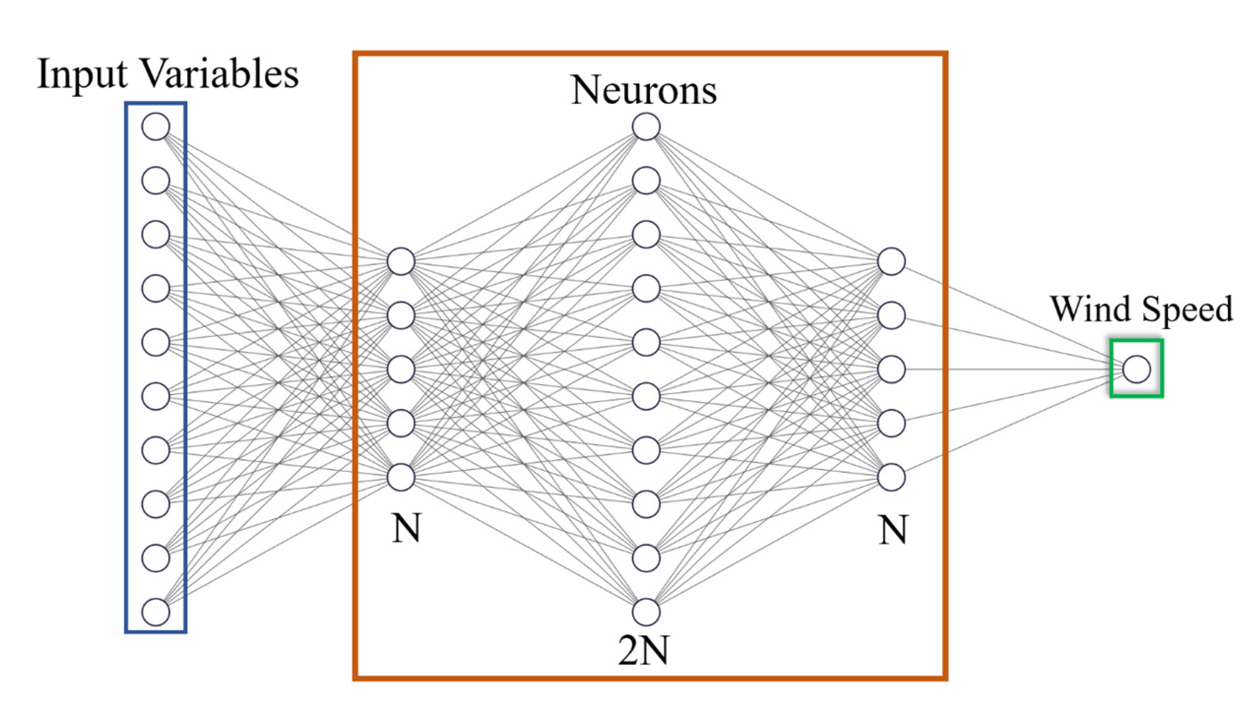
The effects of the number of neurons and activation functions on the performance of ANN wind speed retrieval are analyzed.
The rest of the paper is organized as follows.
Section 2 introduces the GNSS-R variables and then describes the basic principles of the machine learning methods used in this study.
Section 3 provides details of the applied data preprocessing strategies, the data filtering algorithm, and the construction of the machine learning-based model; the experimental results are also presented.
Section 4 discusses the effects of the variables on wind speed retrieval.
Section 5 presents the conclusions.
4. Discussion
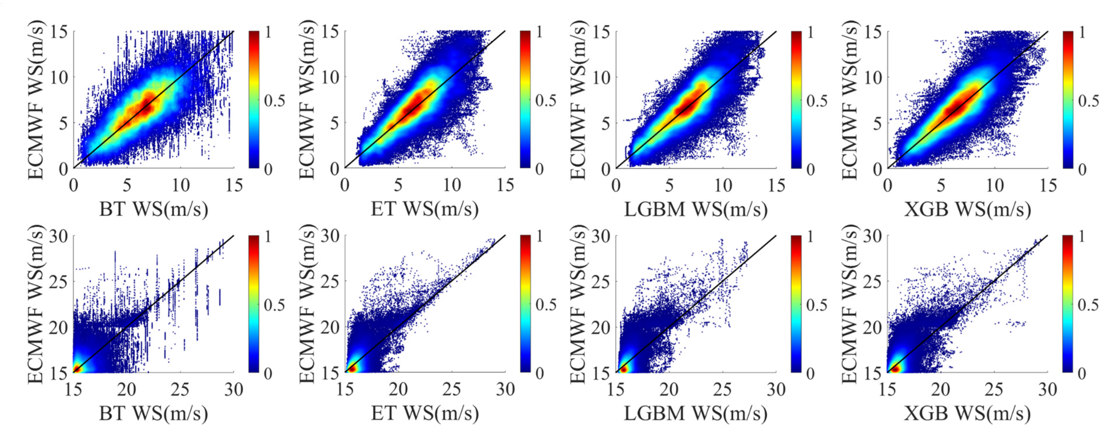
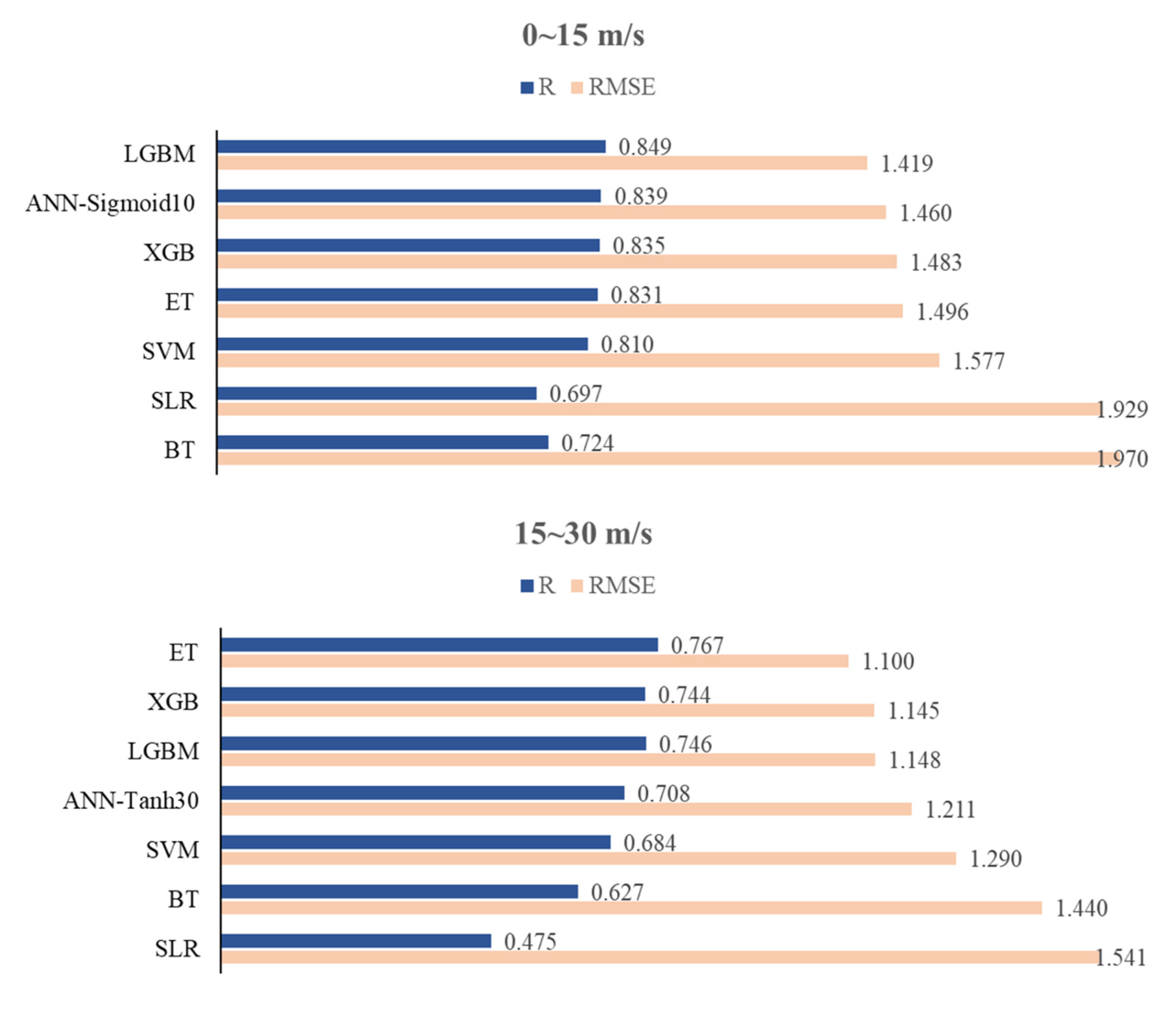
By analyzing the performance of all seven models, it can be concluded that LGBM performed best in the low wind speed interval, while ET performed best in the high wind speed interval. However, the above experimental results do not prove that all the variables in
Table 1 can be used to optimize the performance of the model. On the contrary, some variables may reduce the accuracy of the model. Therefore, it is very important to analyze the effects of different variables. It should be noted that in the high wind speed interval, the data of spaceborne GNSS-R also present different data distributions and characteristics from those in the low wind speed interval, and the roles of the variables were not always consistent. Here, we use the characteristics of XGBoost as the basis for evaluating the effect of each variable. XGBoost uses the average gain (AG) of data splits across all trees to measure the effects of variables [
51]. After model training, by analyzing the XGBoost model structure, the AG related to each variable is defined as:
where
is a variable used in the XGBoost model,
is the number of times that
is used to split the data across all trees and
is the gain value of each tree after splitting with
.
Table 9 shows the AG of each variable in the low and high wind speed intervals, respectively.
Although AG helps to verify the effectiveness of feature selection, it cannot be used as a direct basis thereof. As such, the rationale of
Table 9 needs to be demonstrated through experimental results. In order to analyze the influences of different variables more intuitively, this study constructed 60 models based on ET, XGB and LGBM with different variables. Line charts were used to help in analyzing the influence of these variables. The
x-axis in
Figure 12 indicates the number of variables, which is consistent with the ranking of the effects of variables in
Table 9. For example, in the low wind speed interval, if the number of variables was set at 4, NBRCS, LES, SNR and SWH_swell were used in the modeling; in the high wind speed interval, if the number of variables was set at 3, SWH_swell, NoiseFloor and NBRCS were used in the modeling.
In
Figure 12, the relationship between variables and models can be analyzed clearly. It is obvious that
Figure 12 and
Table 9 are highly consistent. In the low wind speed interval, the AG of NBRCS is much larger than that of other variables, which means that NBRCS is the most important variable in the low wind speed models. In the two subgraphs of the first column of
Figure 12, it is obvious that LES, SNR and SWH_swell improved the performance of the model greatly, as also confirmed in
Table 9. In
Table 9, the AGs of LES, SNR and SWH_swell are significantly greater than those of the other variables. These variables effectively reduced the RMSE of the model and increased the correlation coefficient between the wind speed estimates and the true values of wind speed. In the high wind speed interval, the models were mostly affected by SWH_swell; this may have been due to the degradation of the performance of spaceborne GNSS-R technology in a high wind speed. This result also indicates that, especially in the high wind speed interval, spaceborne GNSS-R technology needs to fuse more reliable auxiliary information to achieve better retrieval results. The contributions of other variables to the model are basically similar. Different from the results of the low wind speed interval, the effects of NoiseFloor and ScatterArea were significantly greater, while the effects of SNR and LES were lower. In the high wind speed interval, the quality of DDM became lower, decreasing the correlation coefficients between sea surface MSS and the variables SNR and LES.
In general, from the above analysis, it is obvious that the results of the models with all variables are the best in both high and low wind speed intervals. In most cases, the accuracy of the model is directly proportional to the number of variables. Additionally, for different modeling methods, the influence of the number of variables was different; for different wind speed intervals, the rankings of the effects of variables were different. The above conclusions may be helpful for the future research of spaceborne GNSS-R sea surface wind speed retrieval.
5. Conclusions
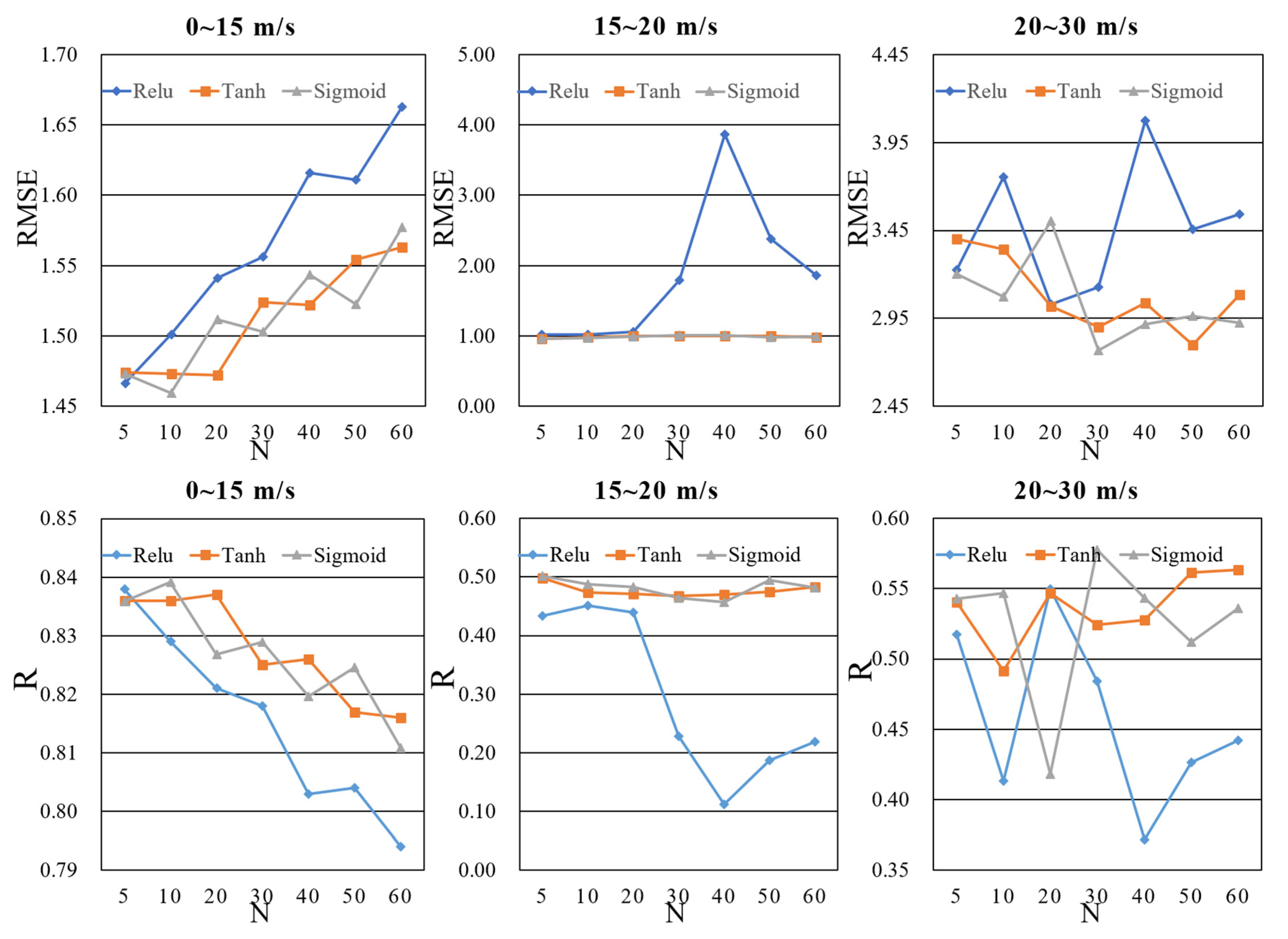
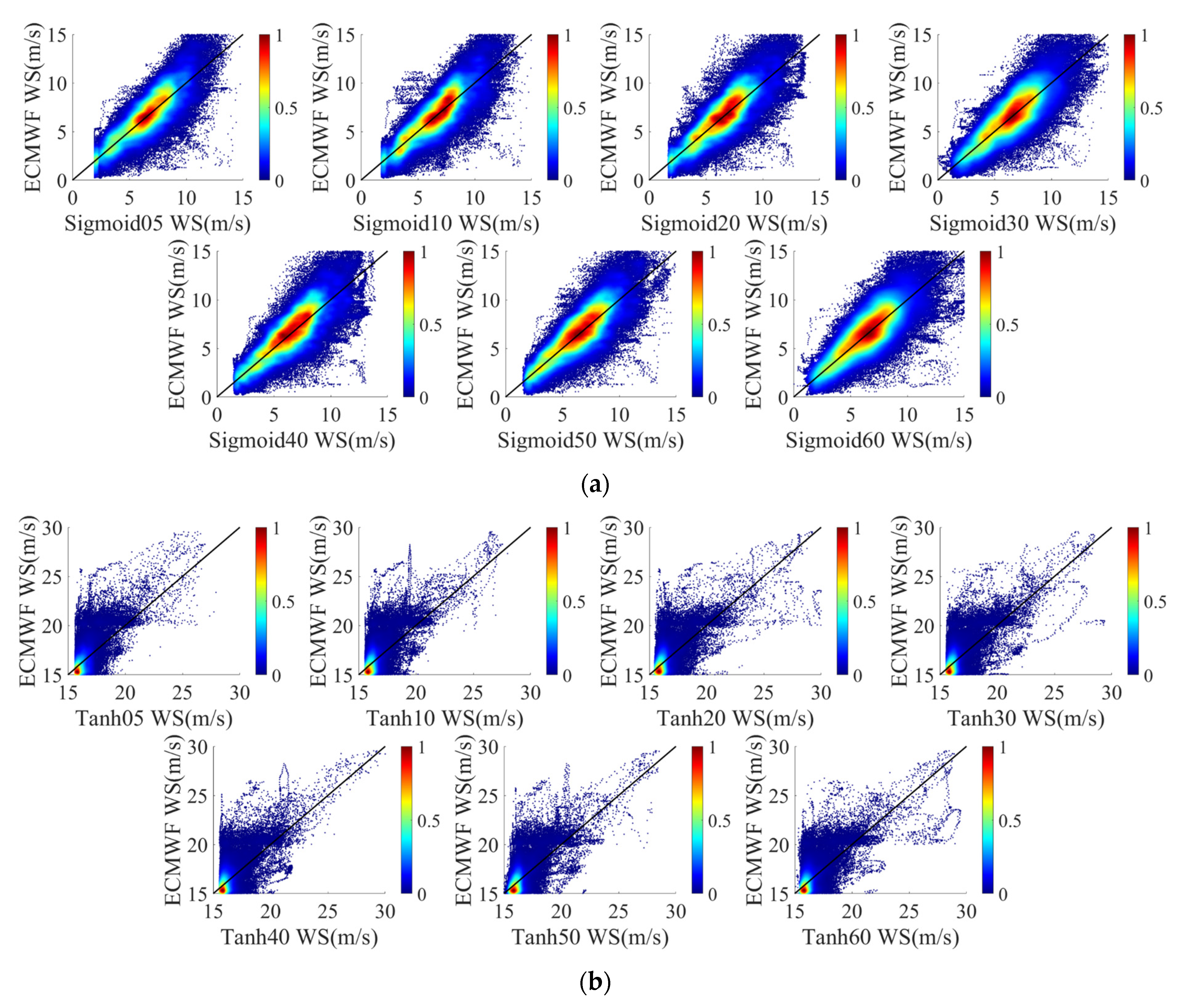
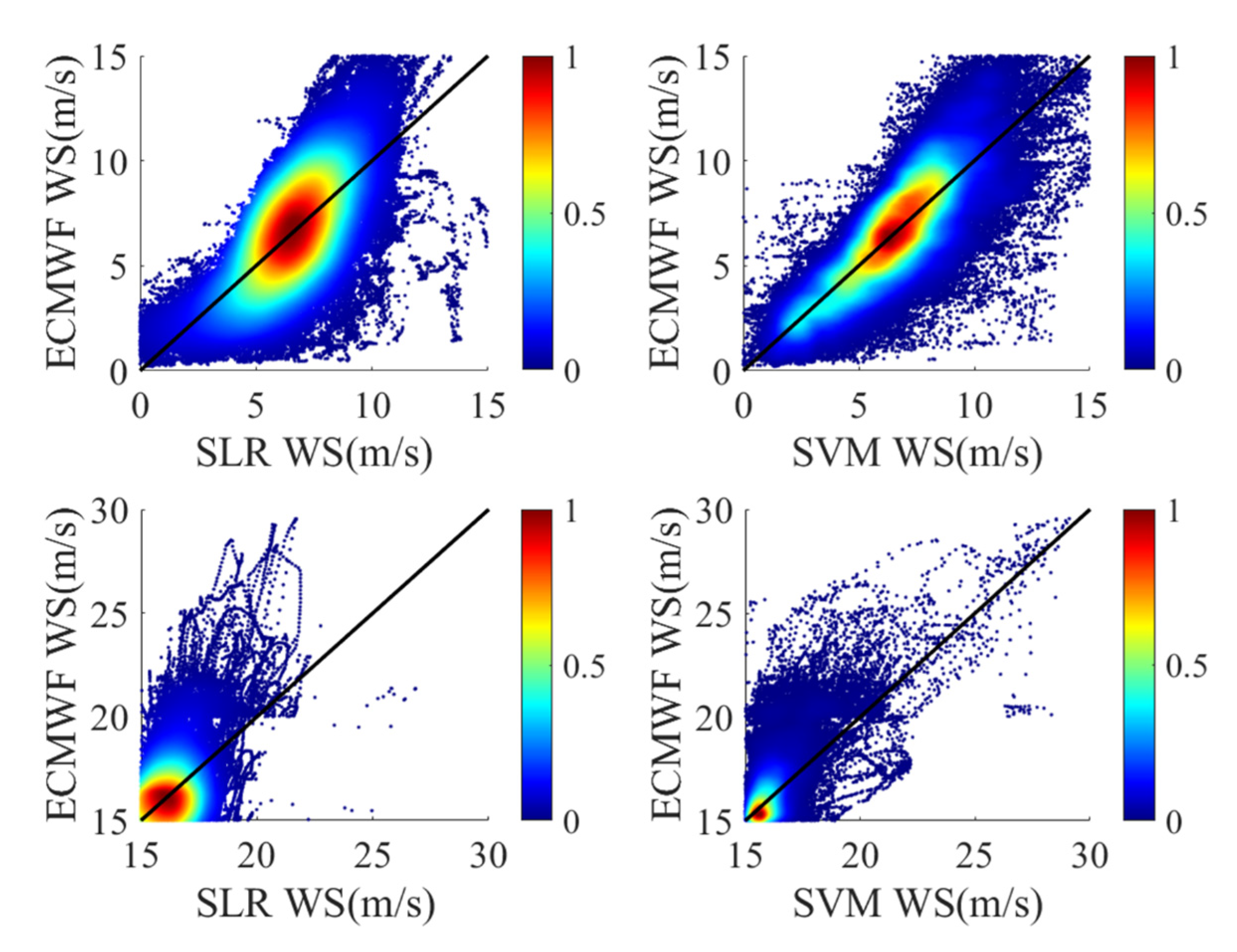
By using machine learning methods, this study investigated wind speed retrieval in different wind speed intervals. Through extensive processing of experimental data, it was observed that different machine learning methods have different properties in different wind speed intervals. In particular, a range of multi-variable models was developed and evaluated. The results showed that the LGBM model performs best with an RMSE of 1.419 m/s and a correlation coefficient of 0.849 in the low wind speed interval (0–15 m/s), while the ET model performs best with an RMSE of 1.100 and a correlation coefficient of 0.767 in the high wind speed interval (15–30 m/s). In addition, through experiments, some characteristics of ANN models were found in wind speed retrieval. In the low wind speed interval, the choice of activation function hardly affects the ANN models, while the increase of the number of neurons significantly reduces the accuracy of the model. In the high wind speed interval, the increase in the number of neurons has little effect on Sigmoid and Tanh, but it has an obvious effect on ReLu.
The effects of the variables used in the wind speed retrieval models described in this paper were analyzed. Through processing experimental data, it was observed that the models with all variables (i.e. NBRCS, LES, SNR, DDMA, Noise Floor, sp_inc_angle, sp_az_body, Instrument Gain, Scatter Area, and SWH_swell) achieved the highest accuracy. In the low wind speed interval, NBRCS, LES, SNR and SWH_swell were the most important variables. In the high wind speed interval, the models were mostly affected by SWH_swell, and the ranking of the effects of variables was very different from that in the low wind speed interval.
Future studies will focus on further performance enhancements of the models developed in this paper. For instance, the accuracy of the model would decrease in the presence of large wind speed and high SWH_swell. It would thus be useful to develop techniques to handle the retrieval of high wind speeds with minimal performance degradation.


 ,
, 


