Article

Nitrogen Balance Index Prediction of Winter Wheat by Canopy Hyperspectral Transformation and Machine Learning

1
College of Natural Resources and Environment, Northwest A&F University, Xianyang 712100, China
2
Department of Soil, Water and Climate, University of Minnesota, Saint Paul, MN 55108, USA
*
Author to whom correspondence should be addressed.
Remote Sens. 2022, 14(14), 3504; https://doi.org/10.3390/rs14143504
Submission received: 9 June 2022 / Revised: 14 July 2022 / Accepted: 19 July 2022 / Published: 21 July 2022
(This article belongs to the Special Issue Proximal and Remote Sensing for Precision Crop Management)

Abstract

:
Nitrogen balance index (NBI) is an important indicator for scientific diagnostic and quantitative research on crop growth status. The quick and accurate assessment of NBI is necessary for farmers to make timely N management decisions. The objective of the study was to estimate winter wheat NBI based on canopy hyperspectral features between 400–1350 nm combined with machine learning (ML) methods in the individual and whole growth stages. In this study, 3 years of winter wheat plot experiments were conducted. Ground-level canopy hyperspectral reflectance and corresponding plant NBI values were measured during the jointing, booting, flowering and filling stages. Continuous removal spectra (CRS) and logarithmic transformation spectra (LOGS) were derived from the original canopy spectra. Sensitive bands and vegetation indices (VIs) highly correlated with NBI under different spectral transformations were selected as hyperspectral features to construct the NBI estimation models combined with ML algorithms. The study indicated that the spectral transformation significantly improved the correlation between the sensitive bands, VIs and the NBI. The correlation coefficient of the sensitive band in CRS in the booting stage increased by 27.87%, reaching −0.78. The leaf chlorophyll index (LCI) in LOGS had the highest correlation with NBI in the filling stage, reaching a correlation coefficient of −0.96. The NBI prediction accuracies based on the sensitive band combined with VIs were generally better than those based on the univariate hyperspectral feature, and the prediction accuracy of each growth stage was better than that of the whole growth stage. The random forest regression (RFR) method performed better than the support vector regression (SVR) and partial least squares regression (PLS) methods. The NBI estimation model based on the LOGS-RFR method in the filling stage could explain 95% of the NBI variability with relative prediction deviation (RPD) being 3.69. These results will provide a scientific basis for better nitrogen nutrition monitoring, diagnosis, and later for field management of winter wheat.

1. Introduction

Nitrogen (N) content is second only to carbon in crops and is an important component of proteins, nucleic acids, enzymes, chlorophyll, and other cellular metabolites [1,2]. Farmers generally agree that high N fertilization ensures crop growth and increases yields [3]. However, N fertilizer that exceeds the needs of the plant is not only detrimental to plant growth, but also causes environmental pollution and fertilizer waste [4,5]. Therefore, adjusting the N application rate according to the needs of crops is a key factor to improve nitrogen utilization efficiency [6,7,8]. The primary task to achieve this goal is to quickly and accurately assess the N status of crops [9,10].
During crop growth, once leaves and plants are deficient in nitrogen, the contents of chlorophyll (Chl) decreases and epidermal polyphenolics (Phen) increase [11]. The nitrogen balance index (NBI) is defined as the ratio of chlorophyll to epidermal flavonoids (Chl/Flav), and it is used for assessing the N nutrition of crops in precision agriculture [12]. Epidermal flavonoids belong to epidermal polyphenolics, which are part of a large branch of epidermal polyphenolics [13]. NBI corresponds to the chlorophyll concentration corrected by the dry leaf mass per unit area [14]. It is considered to be an important fluorescence parameter as well as an indicator of the N content of crops. NBI is much less sensitive to phenology and reflects the N availability better than either Chl or Phen used individually [15]. Cerovic et al. (2015) confirmed that NBI was the best estimator of leaf nitrogen content (LNC) measured by the Dumas or Kjeldahl method with a root mean square error (RMSE) smaller than 2 mg of N g−1 dry weight and proposed NBI threshold values for grapevines under different N deficiency conditions [16]. Generally, the higher the NBI values, the more sufficient the N content, and the higher the nitrogen utilization efficiency [17,18]. It was also capable of indirect evaluation of in-season soil NO3 N accumulation [19], crop yield and crop quality (protein content, etc.) [20]. Chen et al. (2021) found that the NBI was significantly positively correlated with LNC, shoot nitrogen accumulation, and yield. It could be used for rapid N nutrition diagnosis and yield prediction of super high-yield hybrid rice [21]. Recent studies showed that hyperspectral remote sensing technology has become a major development trend in monitoring the N content of crops due to its high spectral resolution, simplicity, effectiveness, and non-destructiveness [22,23,24]. Hyperspectral features, such as reflectance of sensitive band, “three edge” parameters, and vegetation indices (VIs) were used to identify sensitive regions to specific crop parameters [25]. Numerous studies showed the feasibility of using hyperspectral remote sensing for real-time monitoring of crop N nutrition status [26], such as leaf chlorophyll content (LCC) [27], LNC [28], leaf nitrogen accumulation (LNA) [29], plant nitrogen concentration (PNC) [30], plant nitrogen uptake (PNU) [31], nitrogen nutrition index (NNI) [32], etc. VIs by comprehensive analyses on canopy spectral reflectance from visible to near-infrared light were regarded as the most important hyperspectral features for monitoring crop N content. Xu et al. (2021) found that coverage-adjusted spectral indices (CASIs) accurately estimated the LNC of maize [33]. Zhao et al. (2018) developed a normalized difference spectral index (NDSI (R710, R512)) for maize NNI estimation. They found that the performance was better than the existing vegetation indices (ratio vegetation index (RVI) and modified soil adjusted vegetation index (MSAVI)) [34]. The research by Peng et al. (2021) showed that sensitive bands and the VIs derived from different platforms were equally suited as input predictors for assessing plant N status, including the PNU, PNC and NNI [31].
Recently, multiple Vis of hyperspectral features from transformed spectra and machine learning (ML) techniques have been combined and are widely used to build predictive models with improved prediction accuracy. Li et al. (2019) showed that hyperspectral features from log transformation spectra (LOGS) and continuous removal transformation spectra (CRS) could improve the wheat LNC estimation to different degrees compared with raw canopy spectra [35]. Guo et al. (2021) found that the best LNA estimation model could be constructed by support vector machine (SVM) regression when the reflectance values of the chlorophyll absorption band were normalized with the CRS [29]. Additionally, artificial neural network (ANN) and random forest (RF) algorithms all showed promising performance in crop N monitoring using hyperspectral remote sensing [36]. Overall, hyperspectral remote sensing can be used for precision nutrient management to assess plant N status in a real-time manner.
Thus far, less is known about the ability to estimate NBI using hyperspectral remote sensing. Studies have shown that NBI was closely related to VIs that characterize crop growth status [37]. However, limited to a few VIs, we need to add more VIs to reflect the degree of response to NBI. Quemada et al. (2014) found a significant correlation between the transformed chlorophyll absorption in the reflectance index/optimized soil-adjusted vegetation index (TCARI/OSAVI) and NBI based on hyperspectral indices obtained from field observation data and airborne images in the study of N fertilizer implementation in maize [38]. Li et al. (2015) found that the dark color green index (DGCI) was significantly correlated with NBI and could be used to explain 77.1% of the variability in NBI [11]. The challenges are to further confirm the response of sensitive bands and VIs to NBI and increase the estimation accuracy of NBI. Since crop N changes over the course of plant growth, early nitrogen status is closely related to crop growth, while nitrogen status at maturity determines crop yield. Further research should be conducted to understand how accurately it can be estimated during hyperspectral remote sensing under different spectral processing and modeling methods in each growth stage.
Therefore, based on the canopy hyperspectral reflectance of winter wheat, the objectives of this study are to: (1) find the hyperspectral features (sensitive bands and VIs) highly correlated with NBI under different spectral transformations in each growth stage and the whole growth stage; (2) analyze whether the sensitive bands and VIs under transformed spectra can enhance the correlation between original spectra and NBI; (3) explore the potential of ML algorithms in NBI estimation. The research results will provide a technical basis for the potential application of hyperspectral remote sensing technology in N monitoring and diagnosis in winter wheat production.

2. Materials and Methods

2.1. Experimental Design

Field trials of winter wheat were conducted are the Northwest A&F University experimental station in the Yangling Agricultural Demonstration Zone, Shaanxi Province (34°14′N, 108°10′E), and Qinan village, Xianyang City, Shaanxi Province, China (34°38′N, 108°07′E). The soil types in both stations were loam. The common winter wheat cultivar “Xiaoyan 22” was planted in early October and harvested at the end of May of the following year. N, P and K fertilizers in the two experimental sites were broadcast at one time before planting. No top-dressing was applied during the growing season. Field management measures were the same as local conventions.
A total of 40 plots were established in the Qinan experimental station in 2016 (36 small plots and 4 on-farm plots). Three treatments and six levels in each treatment were conducted in 36 small plots. Each treatment had only one nutrient rate being changed. Each plot area was 9 × 10 m. Six N rates (0, 30, 60, 90, 120 and 150 kg/ha), six P rates (0, 22.5, 45, 67.5, 90 and 112.5 kg/ha) and six K rates (0, 15, 30, 45, 60 and 75 kg/ha) were applied and replicated twice. The basal fertilizers for N, P and K treatments were applied with 60 kg/ha K2O and 45 kg/ha P2O5, 60 kg/ha K2O and 90 kg/ha N, and 90 kg/ha N and 45 kg/ha P2O5. In the 4 on-farm plots, each plot was about 480 m2. The rates of N were 0, 60, 120 and 180 kg/ha. The basal P and K fertilizers were 60 and 45 kg/ha.
In 2017 and 2020, 20 small plots were set up at the Northwest A&F University station. Each plot was 5.5 × 6 m. Replicated N and P fertilizer rate trials involved the application of N fertilizer at 0, 45, 90, 135 and 180 kg/ha for each treatment. The application of K fertilizer was 0, 22.5, 45, 67.5 and 90 kg/ha for each treatment.

2.2. Data Collection

2.2.1. Hyperspectral Data Determination

The canopy spectrum of winter wheat in each growth stage was measured by using the SVC HR-1024I field spectroradiometer during the period of 10:30–14:00 in sunny and windless weather. The wavelength range was 350–2500 nm, with spectral resolutions of 3.5, 9.5 and 6.5 nm at 350–1000, 1000–1850 and 1850–2500 nm, respectively [35]. A 25° viewing angle lens was set one meter above the winter wheat canopy and vertically downward during the observation. The sensor was calibrated using a standard whiteboard before each measurement and was set to repeat 10 times during each measurement. Two sample points were taken in the diagonal direction of each plot, and the mean value of the spectral measurements of the sample points was the canopy spectrum of the plot. In this study, the canopy spectrum of winter wheat was measured at the jointing, booting, flowering and filling stages.

2.2.2. Determination of NBI

After canopy hyperspectral measurements, the NBI of winter wheat was determined using Dualex Scientific+ (Force-A, Orsay, Paris, France). Dualex Scientific+ is a new multi-function leaf measuring instrument, which can accurately measure the chlorophyll content of leaves, flavonoids and anthocyanin content of leaf surface in real time non-destructively. The chlorophyll content was calculated from the far-red light absorbed by chlorophyll and the transmittance of near-infrared light as a reference. The flavonoid content and anthocyanin content were calculated from the different ratios of chlorophyll fluorescence in the epidermis of leaves. The nitrogen balance index is the ratio of chlorophyll and flavonoids. When the plant was in a healthy state, the chlorophyll content was high, and the polyphenols (flavonoids) produced at this time were relatively small. Once the plant was deficient in nitrogen, it would affect the synthesis of chlorophyll and produce large amounts of polyphenols (flavonoids). Therefore, by measuring the nitrogen balance index of plants, the nitrogen nutrition status of plants can be quickly and effectively evaluated, which is more advantageous than the traditional single chlorophyll evaluation method [12,39]. The instrument calibration was completed before the NBI measurement following instructions of the manufacturer. Nine fresh leaves from the two sample points were measured and averaged as the NBI value in each plot. Each leaf was measured 3 times from petiole to leaf tip (avoiding the vein part), taking the average as the NBI value of each leaf [13]. Through the experiments, 248 sample data were obtained. The number of samples in each growth stage was 56, 60, 76 and 56.

2.3. Canopy Hyperspectral Transformation

Due to the influence of the instrument itself and background environmental factors, the canopy hyperspectral data contained not only the spectral signals of ground objects but also noise information. Among them, there were several strong absorption interference locations corresponding to moisture of the instrument at 1350–2500 nm. Studies have shown that the spectral reflectance in the visible–near-infrared band was closely related to nitrogen accumulation [23]. Therefore, this study performed an NBI analysis based on hyperspectral reflectance in the range of 400–1350 nm. The collected spectral data were resampled to the interval of 1 nm. With a quadratic polynomial and 9 smoothing points, the Savitzky–Golay smoothing filter was used for fitting and filtering to remove noise from the resampled reflectance spectral curve. The denoised hyperspectral spectrum was labeled as the original spectrum (OS). In this study, two different spectral transformations were performed to extract the sensitive bands and VIs. CRS was obtained by normalizing the absorption valley in the spectral curve onto the continuum line of the absorption valley, so that the spectral absorption characteristics and hyperspectral features could be better analyzed and selected [40]. LOGS was determined by calculating a log function of the spectral reflectance’s reciprocal, which could improve the sensitivity of canopy spectra to NBI [41].

2.4. Selection of VIs

The VI is defined as the combination of reflectance in a certain specific wavelength, which is related to leaf pigment, photosynthesis, and plant growth. Twenty-three VIs highly correlated with plant N status were selected for this analysis. The calculation and literature source of each VI are presented in Table 1.

2.5. Model Development

Hyperspectral features, including sensitive bands and vegetation indices (VIs), highly correlated with NBI under different spectral transformations were selected as independent variables. The Dualex-measured NBI values were the dependent variable. The univariate regression (UR), partial least squares regression (PLS), random forest regression (RFR) and support vector regression (SVR) methods were used to construct the NBI estimation models.

2.5.1. Univariate Regression

Univariate regression refers to a method in which there is only one independent variable correlated with one dependent variable [41]. In this study, the hyperspectral feature was used as an independent variable to build the NBI univariate regression model (NBI-UR), in which the exponential, linear, logarithmic, polynomial and power functions were tried.

2.5.2. Partial Least Squares Regression

PLS is a combination of multiple linear regression analysis, canonical correlation analysis and principal component analysis. It is a commonly used multivariate statistical regression method to deal with the highly collinear variables, which is useful in dealing with a small number of samples in the spectral analysis [45]. In this study, the number of latent variables is selected on the basis of the standard error of leave-one-out cross-validation. Modeling and parameter optimization were performed based on Matlab2019a software and Minitab19 software.

2.5.3. Random Forest Regression

RFR is an ensemble ML method for building decision trees by bootstrap sampling and random subspace methods. During the operation, only randomly selected predictors are used for each tree. The final prediction result is determined by the average of all decision trees. The “ntree” (the number of decision trees) and “mtry” (the number of segmentation nodes) are two key parameters that need to be optimized in RFR. In this study, “mtry” was set to 1/3 of the number of independent variables, as suggested by Breiman (2018) [46], and “ntree” was trained through tuneGrid, and the value of “ntree” as 500 was finally selected. This process was implemented in the randomForest package of the R statistical software.

2.5.4. Support Vector Regression

As an ML method, SVR transforms the actual problem into a high-dimensional feature space and constructs a linear decision function in high-dimensional space corresponding to a nonlinear decision function in the original space. It can subtly solve the dimensional problem and ensure good generalization ability, and the algorithm complexity is not related to the sample dimension [47]. In this study, the radial basis function (RBF) kernel and grid search method were used to select the optimal parameters for SVR-based NBI model building. The penalty parameter (C) and the kernel parameter (γ) were optimized within [2−1–21] and [e−2–e4], respectively. The process was carried out in the e1071 package of the R statistical software.

2.6. Evaluation Metrics for Model Accuracy

The sample data of each growth stage were randomly divided into a modeling dataset and a validation dataset according to the radio of 2:1. The dataset in each stage was pooled together as the dataset of the whole growth stage (Sall). The description of NBI is shown in Table 2. The determination coefficient (R2), RMSE and relative prediction deviation (RPD) were used for model verification. R2 and RMSE indicate the degree of fit and the degree of deviation between the predicted and the measured NBI values. RPD evaluates the predictive ability of a model by measuring the relative deviation between the predicted and measured values. It is an indicator of the reliability and usefulness of the model [48]. The higher the R2 and the lower the RMSE, the better the prediction model for NBI. Models with RPD < 1.5 are not convincing, models with 1.5 < RPD < 2.0 have a good ability to estimate samples, and RPD > 2.0 indicates that the model has an excellent ability to interpret the dependent variable. The calculation of RPD is shown in Formula (1):
RPD = SD/RMSE
where SD and RMSE are the standard deviation and root mean square error of the validation set respectively.

3. Results

3.1. Descriptive Analysis of Nitrogen Balance Index

Ground truth measurement statistics of winter wheat nitrogen balance index (NBI) in each growth stage are shown in Table 2. NBI values ranged from 10.16 to 33.39, and the coefficient of variation varied from 14.67% to 28.99%. The greatly varying NBI values of winter wheat reflect the effective utilization of N in different growth stages. N accumulated continuously before the booting stage. The mean values of NBI decreased from the booting to the filling stage due to the dilution effects [49]. The largest coefficient of variation was found in the filling stage, with values of 28.99% in the modeling set and 28.57% in the validation set. The coefficient of variation values were relatively uniform at other growth stages, indicating moderate temporal variation. The small difference between modeling and validation sets in mean and standard deviation metrics enhanced the feasibility of the study.

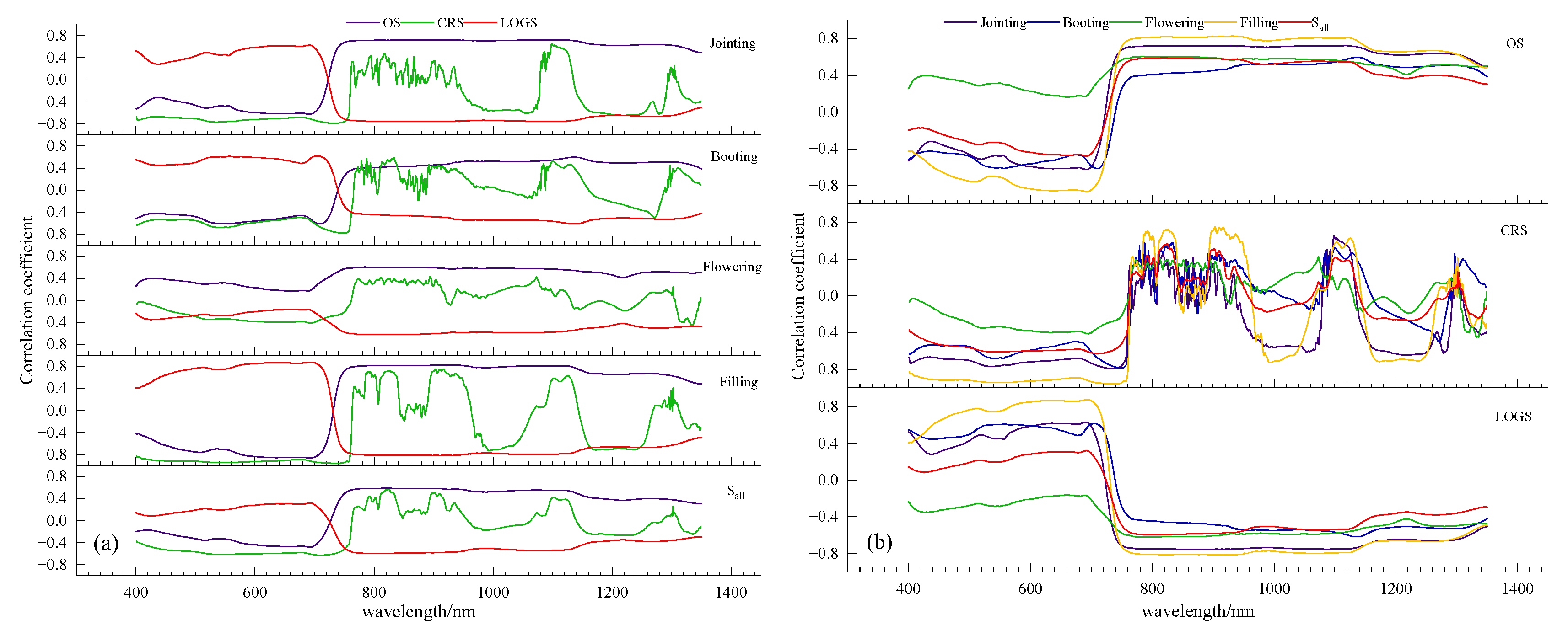
3.2. Hyperspectral Features and Nitrogen Balance Index

3.2.1. Sensitive Bands and NBI

Figure 1 shows the correlation coefficient between the transformed spectra and ground truth NBI measurements in each growth stage of winter wheat. Figure 1a shows that the correlation coefficient values were quite different from the visible and near-infrared bands. The significant change at the red edge indicated that spectral reflectance in this region was particularly sensitive to N content in crop leaves [29]. At the jointing, booting, filling and Sall stages, the OS was positively correlated with NBI below 760 nm and negatively correlated above 760 nm. The OS and NBI were always positively related at the flowering stage. Under the LOGS, the correlation was opposite to that of OS in each growth stage. The correlation between the CRS and NBI fluctuated strongly. The CRS and LOGS increased differences in the correlation coefficient for visible light, especially at the flowering stage (Figure 1b). According to the principle of highest correlation, the sensitive band positions of each transformation spectrum in each growth stage were screened as shown in Table 3. All the sensitive bands passed the significance test. The locations of sensitive bands were in the range of 692–1336 nm, 10 of which were in the visible light region. The sensitive bands of CRS were negatively correlated with NBI in each growth stage. The highest correlation coefficient values with NBI at the jointing, booting, filling and Sall stages were given by the CRS, with values of −0.79, −0.78, −0.95 and −0.63, respectively. LOGS performed the best in the flowering stage, and the correlation coefficient was −0.62. On the whole, the correlation between the transformed spectrum and NBI was stronger than that of the original canopy spectrum, indicating that the spectral transformation significantly improved the sensitivity of the canopy spectrum to NBI.

3.2.2. VIs and NBI

Figure 2 showed the correlation between VIs and NBI under different transformed spectra of winter wheat in different growth stages. In the jointing stage, all the VIs except for TCARI and NDSI in OS, and NDSI and mSR705 in CRS, passed the 0.01 significance test. In the booting stage, the NRI performed poorly under different transformations. In the flowering stage, 47.83%, 43.48% and 82.61% of VIs in OS, CRS, and LOGS, respectively, were correlated with NBI at the significance level of 0.01. In the filling stage, except for DCNI in LOGS, and mSR705 in CRS, all the other VIs were significantly correlated with NBI. Most of the absolute values of the correlation coefficient between VI and NBI were above 0.8, indicating a good response of VI to NBI in filling stage. In the Sall stage, only the NDSI in OS and CRS failed the significance test of 0.01. Overall, the spectral transformation had little effect on improving the correlation between VI and NBI. VIs that passed 0.01 significance for all growth stages included OSAVI, GNDVI, NDCI, GRVI, NPCI642 and LCI.

3.3. NBI Estimation Model

After analyzing the correlations between 23 VIs and NBI under different transformed spectra in each growth stage, it was found that the correlation coefficient values between VIs and NBI at each growth stage were quite different; thus, it was not appropriate to choose a unified VI for further research, and it was necessary to use different VIs for further research. Therefore, in combination with the sensitive band, the top five VIs significantly correlated with NBI at the 0.01 level were selected in each growth stage to build the multivariate models for NBI. Since there were two VIs with the same correlation coefficient in the jointing stage, seven characteristic parameters were finally involved in the model construction. Six characteristic parameters were used for the model construction in each of the other growth stages. The selected hyperspectral features are listed in Table 4.

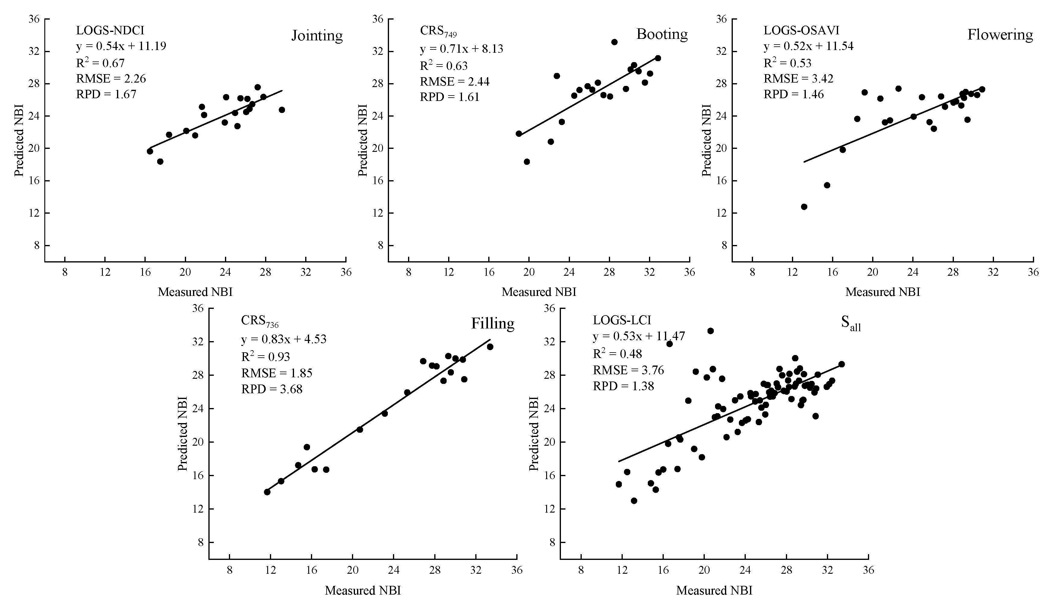
3.3.1. Univariate Regression Model for NBI Estimation (NBI-UR)

Taking the sensitive band and the optimal VI in OS, CRS and LOGS as independent variables, a univariate regression model of winter wheat NBI in each growth stage was established. Figure 3 illustrates the R2 and RMSE of each estimation model, and the explanatory power of the best estimation model for each growth stage is presented in Figure 4. Under different transformation spectra, the explanatory power of NBI at the filling stage was the highest, followed by the jointing stage and the booting stage, and the NBI explanatory power at the flowering stage and the Sall stage was poor.
From the jointing to the filling stage, the best hyperspectral feature for NBI was LOGS-NDCI, CRS749, LOGS-OSAVI and CRS736, which explained 67%, 63%, 53% and 93% of the variation in NBI, respectively. The best parameter in the Sall stage was LOGS-LCI, which explained only 48% of the variability in NBI. On the whole, most of the NBI-UR models were simple nonlinear models. In each growth stage, the models constructed by the VI were better than the sensitive band with OS. The explanatory power of the NBI estimation models constructed by univariate parameters under CRS and LOGS was higher than that of the OS models. It was expected that VIs could eliminate the influence of vegetation coverage and growth status to a certain extent through the combination of characteristic bands, and they could improve the responsiveness to NBI [50]. However, the models constructed with the VI did not significantly improve the estimation ability of NBI, which was consistent with the previous studies on LNA in winter wheat with hyperspectral reflectance [29].

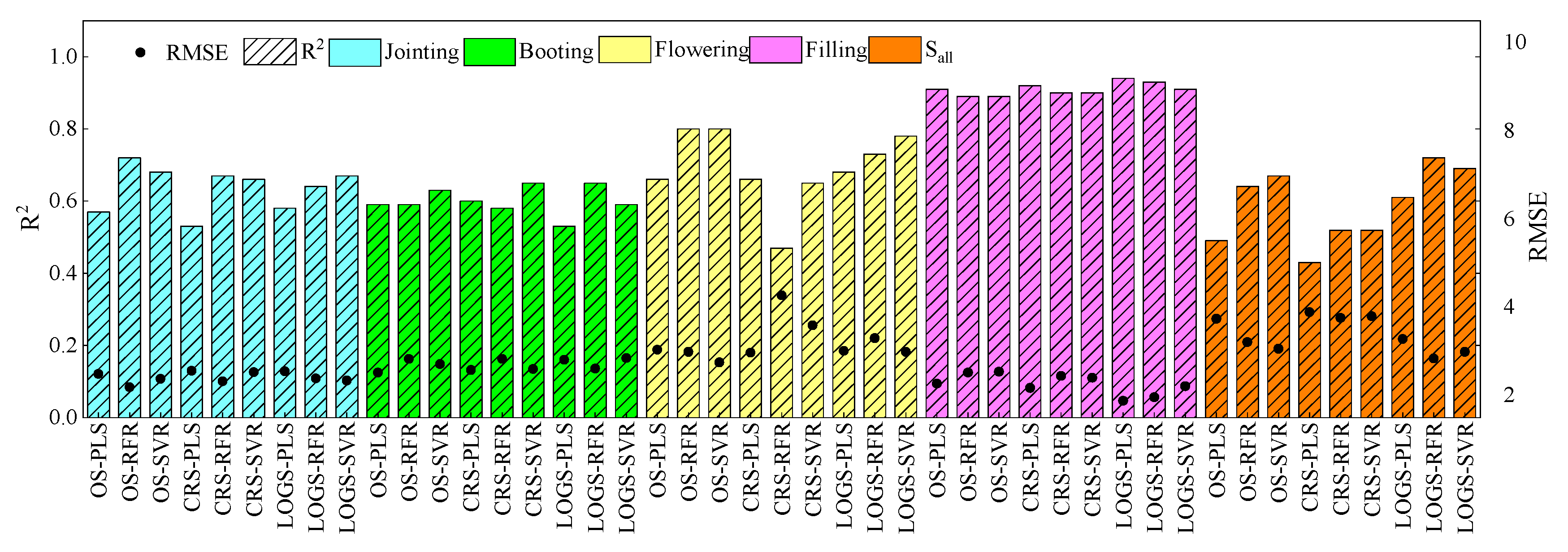
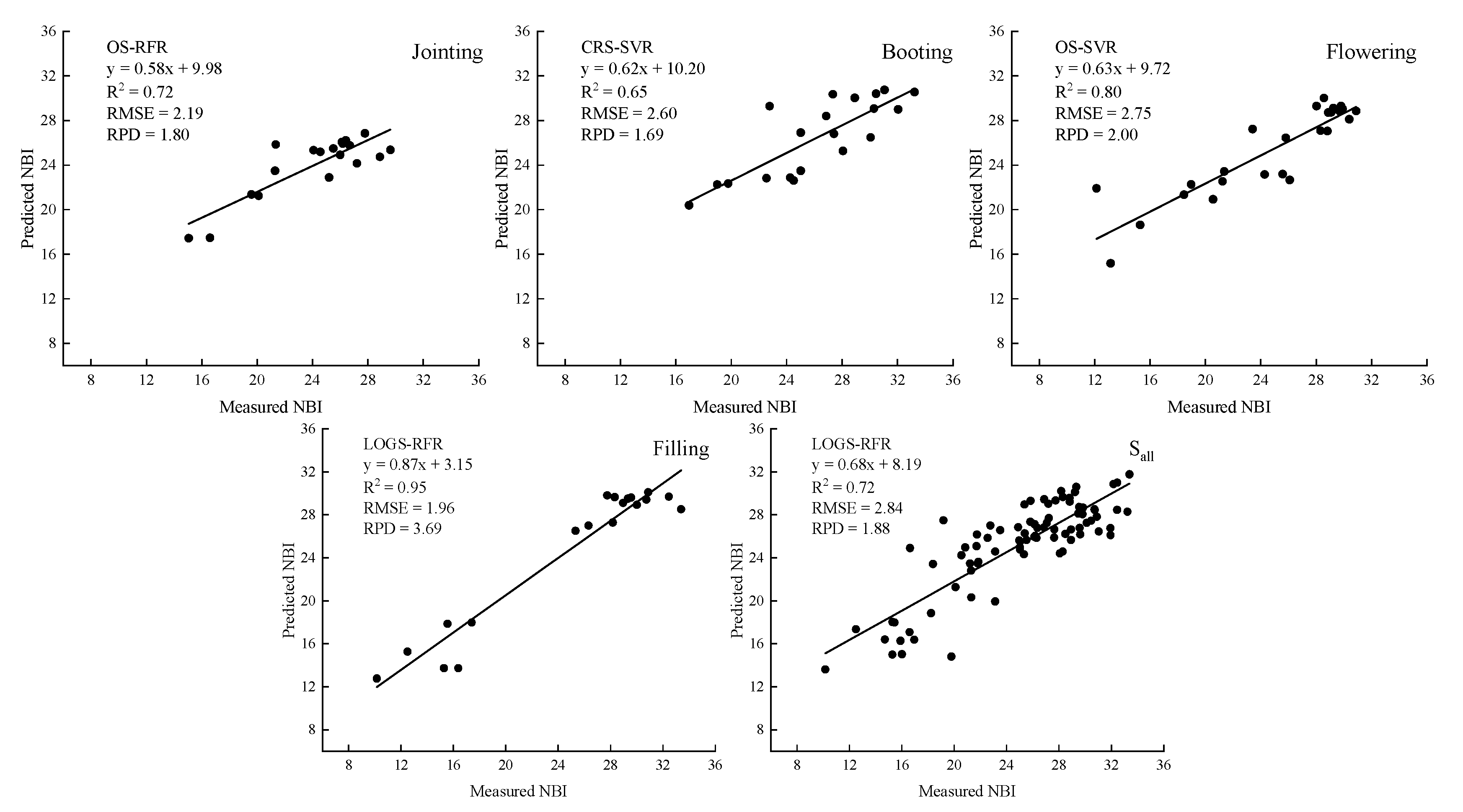
3.3.2. Multivariate Regression Model for NBI Estimation (NBI-MR)

Previous studies have demonstrated that the explanatory power of the estimation model constructed using multiple VIs was higher than for models constructed using a single VI. Using multiple VI could effectively improve the prediction power of physiological and biochemical parameters of crops [51]. In this study, the multivariate regression (MR) models were constructed by using the sensitive band combined with the optimal VI under the different transformation spectrums in each growth stage. The R2 and RMSE of each estimation model are shown in Figure 5, and the scatter plot of the best estimation model for each growth stage is shown in Figure 6.
From the jointing to the filling growth stage, the best multivariate models for predicting NBI were OS-RFR, CRS-SVR, OS-SVR and LOGS-RFR, which could explain 72%, 65%, 80% and 95% of the NBI variation, respectively (Figure 5). All the NBI-MR models in the filling stage had an excellent ability to estimate NBI. In the Sall stage, the R2 of the best estimation model was improved from 0.48 (LOGS-LCI model) to 0.72 (LOGS-RFR model). Overall, the combination of multiple variables improved the explanatory power of NBI estimation. As a multiple regression model, the performance of PLS was better than that of the univariate regression model in each growth stage. The explanatory power of the winter wheat NBI model constructed based on an ML algorithm was higher than that of the PLS model, and the distribution of the measured and the estimated NBI values was closer to the 1:1 line. The RFR model showed high prediction power in the modeling sets of each and the whole growth stage, but for the validation set, the RFR and SVR models performed unevenly in different growth stages, which may indicate an overfitting problem in the modeling process [45].

3.4. Model Accuracy Comparison

As shown in Figure 7, the RPD values of the best NBI-UR models were 3.68, 1.67, 1.61, 1.46 and 1.38 at the filling, jointing, booting, flowering and Sall stages, respectively. The prediction accuracy results of the NBI-UR models demonstrated that the estimation ability was better in each growth stage than that in the Sall stage (Figure 4). The NBI-UR models in the filling stage could accurately evaluate the NBI distribution. In this stage, the RPD of all sets of the NBI-UR models was greater than 2.0, except for the sensitive band at 692 nm in OS. The RPD values of each model based on the VI in LOGS at the jointing stage and the sensitive band at 749 nm in CRS at the booting stage were higher than 1.50. All the NBI-UR models in the flowering and Sall stage were less than 1.5.
As shown in Figure 8, the RPD values of the best NBI-MR models were 3.69, 2.00, 1.88, 1.80 and 1.69 at the flowering, booting, Sall, filling and jointing stages, respectively. The NBI model by LOGS-RFR in the filling stage was outstanding, with the best RPD at 3.69, and the lowest RPD greater than 2.0. Some of the NBI estimation models had a good explanatory ability with RPD values greater than 1.5 and less than 2.0 at other growth stages. The RFR algorithm had better accuracy than PLS and SVR in NBI estimation.
From the comparison of the best NBI-UR and NBI-MR models, the NBI-MR models significantly improved the estimation accuracy of NBI in each growth stage, especially in the flowering and Sall stages (Figure 9). The NBI-MR estimation models significantly improved the estimation accuracy of NBI in each growth stage (Figure 9), especially during the flowering and the whole growth stages. The R2 and RPD of the best estimation models for the flowering stage were improved from 0.53 (LOGS-OSAVI) to 0.80 (OS-SVR), and from 1.46 to 2.00, respectively. The R2 of the Sall stage was increased from 0.48 (LOGS-LCI) to 0.72 (LOGS-RFR), and the RPD was increased from 1.38 to 1.88. On the whole, estimating NBI in each growth stage was more accurate than in the whole growth stage (Sall), and the performance in each growth stage was significantly different. The NBI estimation model in the filling stage was the highest in both the NBI-UR and NBI-MR models. The best NBI-MR model based on the RFR algorithm could be used for accurate NBI estimation in each growth stage.

4. Discussion

N is a key nutrient required to maintain crop growth. NBI can quickly provide feedback on the N nutrition of crops. For real-time assessment and monitoring of NBI, studies have been conducted using passive and active remote-sensing techniques [18,19]. In this study, the relationship between winter wheat canopy hyperspectral reflectance at 400–1350 nm and NBI estimation was explored. Based on sensitive bands and VIs, NBI-based N monitoring models were constructed in different growth stages using different regression methods.

4.1. Feasibility of Sensitive Bands and VIs to Estimate NBI

The positions of the sensitive bands in each growth stage and Sall stage were roughly the same both in the visible and near-infrared regions (Table 3), which might be attributed to the fact that the spectral reflectance in these regions was closely related to the Chl of winter wheat [52]. Meanwhile, chlorophyll content proved to be the best predictor for monitoring N status [22]. The most important criteria for choosing a VI are high correlation with the target variable (NBI in this case) and low sensitivity to other confounding factors [53]. The 23 VIs selected in the study were highly correlated with NBI because NBI was quantitatively correlated with LNC [15]. However, these VIs responded differently across different growth stages. This study found that some VIs performed better in all growth stages of winter wheat and were selected as the best VI in some growth stages, such as NDRE, CI red and LCI. Among them, the NDRE was the ratio of near-infrared and red edge reflectance, which could more sensitively reflect the chlorophyll content of vegetation and could still be used as one of the options in future research.
It was found that sensitive bands and VIs under transformed spectra (CRS and LOGS) were more sensitive to NBI than the OS. The correlation between the sensitive bands and VIs with NBI in the flowering growth stage was inferior to that of other individual growth stages, despite the spectral transformation. The main reason was that in this growth stage, there was senescence in canopy leaves, which led to a decline in the quality of spectral information, indicating that crop status was significantly different between different growth stages and seasons [54]. This did not mean that the selected VI had a weak correlation with NBI. After integrating data across all growth stages, it was found that the correlation between NBI and a single VI decreased significantly. Individual VI had varying relationships with canopy characteristics at different growth stages, likely as a result of changes in canopy biomass and LNC. These changes in VI accuracy affected the accuracy of predicting NBI as a whole. A similar phenomenon was also found in the study by Gitelson et al. (2017) [55].

4.2. Potential for Estimating NBI in Each Growth Stage

LNC changes over the course of plant growth. Monitoring crop N status at different time periods is of interest to guide crop management, as the development of growth stages is accompanied by changes in canopy structure and N allocation [56]. For early growth stages, monitoring N status is critical to help guide fertilization strategies [57], while in the growing stage near maturity, N status will determine the quality of the grain [58]. Previous studies showed different views on the optimal growth stage for physical and chemical parameter inversion in different crops. Li et al. (2021) explained that the flowering and filling stages were the best timing for leaf area index (LAI) estimation [59]. The results of Zhang et al. (2021) revealed that the use of the whole growth stage model could obtain a better prediction effect of the above-ground biomass of maize than any individual growth stage [60]. Cerovic et al. (2015) recommended performing leaf N diagnosis somewhere between flowering and canopy closure [16].
Our results revealed that the NBI estimation accuracy was higher in individual growth stages than across all growth stages, and the NBI prediction model in the filling growth stage was stable and had the highest accuracy. This might be because the NBI takes into account not only the surface-based variability in N needs in the photosynthetic machinery but also the variation in leaf mass per area (LMA). Studies have shown that when biomass dominates canopy reflectivity, the rate of aboveground biomass production exceeded the rate of N uptake by plants. Conversely, when plant N dominates canopy reflectivity, biomass increased more slowly [61]. Therefore, N content was sufficient when winter wheat gradually approached the mature stage. The accurate monitoring of N nutrition in the filling stage is of great significance for the prediction of winter wheat grain quality in the later growth stages [62]. LNA at the jointing and booting stages accounts for almost half of the total N accumulation in these key periods for the formation of crop yield and quality and has large implications for precision fertilization and field management decisions [63]. During these periods, it is necessary to provide timely feedback to farmers on nitrogen status. Therefore, improving the NBI estimation accuracy at these stages is the most important task in future research. We speculate that spectral information that highlights seasonally important growth stage features and spatial texture features can be studied to further improve the prediction accuracy of NBI monitoring.

4.3. Model Selection for NBI

In this paper, the NBI-UR and NBI-MR models were used to estimate the NBI of winter wheat. Only a few sensitive bands and VIs met the estimation accuracy requirements (RPD > 1.5) in the NBI-UR models. NBI-MR models provided better performance than NBI-UR models. For example, LOGS-OSAVI in the NBI-UR models was the best for predicting NBI in the flowering stage with R2 and RPD values of 0.53 and 1.46, respectively. In contrast, the OS-SVR in NBI-MR models greatly improved the NBI accuracy with R2 and RPD values of 0.80 and 2.0, respectively. A significant improvement also was found during the Sall stage. The reason why the NBI-MR model performed better in each growth stage was that the MR model involved multiple hyperspectral features and fully exploited the potential of hyperspectral data information. However, different MR methods yielded highly variable estimation accuracy. The PLS model is a promising technique that could be integrated into crop monitoring systems. Although there was a certain overfitting phenomenon in machine learning, they were more suitable for solving some nonlinear problems as long as the parameters were adjusted accurately [41]. Wang et al. (2020) compared the effects of MK-SVR, multiple linear regression, PLS, and neural network methods in estimating leaf nitrogen concentration and found that the MK-SVR model was the most accurate [64]. Studies confirmed that the SVR and RFR models had similar advantages in estimating orchard apple chlorophyll content [25]. Our results showed that although the NBI-UR model was computationally simple and highly interpretable, its accuracy and reproducibility were low due to less use of rich spectral information. Thus, the NBI-UR models were not recommended. Compared with the NBI-MR model, the PLS, RFR and SVR models could use more band information to establish the model, which had higher accuracy and better stability in estimating NBI. Overall, the ML methods in this study performed better in the estimation of NBI in different growth stages, and the RFR model had the highest accuracy in each growth stage.

4.4. Challenges and Future Research

Based on the commonly used sensitive bands and VIs related to nitrogen, the NBI estimation models for different growth stages and the whole growth stage were constructed in this study. Although good prediction accuracy has been achieved, in terms of sensitive band screening, the canopy hyper-spectra may not be expressed prominently. New algorithms, such as successive projections algorithm (SPA) [65], uninformative variable elimination (UVE) [66] and competitive adaptive reweighted sampling (CARS) [67], could be combined to further improve the accuracy and stability of the NBI prediction, especially in the key growth stages. In addition, further verification research based on different locations and years is needed to expand the applicability of the NBI models.

5. Conclusions

Canopy spectroscopy can be used to estimate the NBI of winter wheat crops and provide effective information to help decide on N fertilization in precision farming systems. This study showed that from the jointing stage to the filling stage, the sensitive bands of the original hyperspectral of NBI located at 929, 709, 748, 692 and 817 nm, and the correlation coefficients with NBI were 0.72, −0.61, 0.60, −0.87 and 0.59, respectively. Spectral transformation significantly improved the correlation between the sensitive bands and NBI. The prediction accuracies of the NBI-MR models based on the sensitive band combined with the VIs were better than that of the NBI-UR models. The best NBI estimation model was obtained by the LOGS-RFR method in the filling stage (R2 = 0.95, RPD = 3.69). This study can provide a more accurate NBI estimation model for monitoring the nitrogen status of winter wheat and can provide a theoretical basis for subsequent crop yield and quality research.

Author Contributions

Conceptualization, K.F.; methodology, K.F.; software, K.F.; validation, K.F. and F.L.; formal analysis, K.F.; investigation, K.F., X.C. and Z.L.; resources, F.L.; data curation, K.F., X.C. and Z.L.; writing—original draft preparation, K.F.; writing—review and editing, K.F., F.L. and D.J.M.; visualization, K.F.; supervision, F.L.; project administration, F.L.; funding acquisition, F.L. All authors have read and agreed to the published version of the manuscript.

Funding

This research was funded by the National Natural Science Foundation of China (41701398) and the Fundamental Research Funds for the Central Universities (2452017108).

Data Availability Statement

Data sharing is not application to this article.

Conflicts of Interest

The authors declare no conflict of interest.

References

  1. Marschner, H. Marschner’s Mineral Nutrition of Higher Plants; Academic Press: Cambridge, MA, USA, 2011. [Google Scholar]
  2. Krapp, A. Plant nitrogen assimilation and its regulation: A complex puzzle with missing pieces. Curr. Opin. Plant Biol. 2015, 25, 115–122. [Google Scholar] [CrossRef]
  3. Bracke, J.; Elsen, A.; Adriaenssens, S.; Vandendriessche, H.; Van Labeke, M.-C. Utility of proximal plant sensors to support nitrogen fertilization in Chrysanthemum. Sci. Hortic. 2019, 256, 108544. [Google Scholar] [CrossRef]
  4. Molla, T.; Abera, G.; Beyene, S. Effects of nitrogen fertilizer and mulch application on growth performance and pod yields of hot pepper (Capsicum annuum L.) under irrigated condition. Int. J. Plant Soil Sci. 2019, 27, 1–15. [Google Scholar] [CrossRef]
  5. Aminifard, M.H.; Bayat, H. Influence of different rates of nitrogen fertilizer on growth, yield and fruit quality of sweet pepper (Capsicum annum L. var. California Wander). J. Hortic. Postharvest Res. 2018, 1, 105–114. [Google Scholar]
  6. Arregui, L.; Quemada, M. Strategies to improve nitrogen use efficiency in winter cereal crops under rainfed conditions. Agron. J. 2008, 100, 277–284. [Google Scholar] [CrossRef]
  7. Meisinger, J.J.; Schepers, J.; Raun, W. Crop nitrogen requirement and fertilization. Nitrogen Agric. Syst. 2008, 49, 563–612. [Google Scholar]
  8. Gebbers, R.; Adamchuk, V.I. Precision agriculture and food security. Science 2010, 327, 828–831. [Google Scholar] [CrossRef]
  9. Thompson, R.; Gallardo, M.; Voogt, W. Optimizing nitrogen and water inputs for greenhouse vegetable production. In Proceedings of the XXIX International Horticultural Congress on Horticulture: Sustaining Lives, Livelihoods and Landscapes (IHC2014), Brisbane, Australia, 17–22 August 2014; pp. 15–30. [Google Scholar]
  10. Fox, R.H.; Walthall, C.L. Crop monitoring technologies to assess nitrogen status. Nitrogen Agric. Syst. 2008, 49, 647–674. [Google Scholar]
  11. Li, J.; Zhang, F.; Qian, X.; Zhu, Y.; Shen, G. Quantification of rice canopy nitrogen balance index with digital imagery from unmanned aerial vehicle. Remote Sens. Lett. 2015, 6, 183–189. [Google Scholar] [CrossRef]
  12. Cartelat, A.; Cerovic, Z.; Goulas, Y.; Meyer, S.; Lelarge, C.; Prioul, J.-L.; Barbottin, A.; Jeuffroy, M.-H.; Gate, P.; Agati, G. Optically assessed contents of leaf polyphenolics and chlorophyll as indicators of nitrogen deficiency in wheat (Triticum aestivum L.). Field Crops Res. 2005, 91, 35–49. [Google Scholar] [CrossRef]
  13. Zhang, K.; Liu, X.; Ma, Y.; Zhang, R.; Cao, Q.; Zhu, Y.; Cao, W.; Tian, Y. A comparative assessment of measures of leaf nitrogen in rice using two leaf-clip meters. Sensors 2019, 20, 175. [Google Scholar] [CrossRef] [Green Version]
  14. Dong, T.; Shang, J.; Chen, J.M.; Liu, J.; Qian, B.; Ma, B.; Morrison, M.J.; Zhang, C.; Liu, Y.; Shi, Y. Assessment of portable chlorophyll meters for measuring crop leaf chlorophyll concentration. Remote Sens. 2019, 11, 2706. [Google Scholar] [CrossRef] [Green Version]
  15. Cerovic, Z.G.; Masdoumier, G.; Ghozlen, N.B.; Latouche, G. A new optical leaf-clip meter for simultaneous non-destructive assessment of leaf chlorophyll and epidermal flavonoids. Physiol. Plant. 2012, 146, 251–260. [Google Scholar] [CrossRef]
  16. Cerovic, Z.G.; Ghozlen, N.B.; Milhade, C.; Obert, M.; Debuisson, S.; Moigne, M.L. Nondestructive diagnostic test for nitrogen nutrition of grapevine (Vitis vinifera L.) based on dualex leaf-clip measurements in the field. J. Agric. Food Chem. 2015, 63, 3669–3680. [Google Scholar] [CrossRef]
  17. Agati, G.; Tuccio, L.; Kusznierewicz, B.; Chmiel, T.; Bartoszek, A.; Kowalski, A.; Grzegorzewska, M.; Kosson, R.; Kaniszewski, S. Nondestructive optical sensing of flavonols and chlorophyll in white head cabbage (Brassica oleracea L. var. capitata subvar. alba) grown under different nitrogen regimens. J. Agric. Food Chem. 2016, 64, 85–94. [Google Scholar] [CrossRef]
  18. Liu, Y.; Wang, J.; Yao, X.; Shi, X.; Zeng, Y. Diversity Analysis of Chlorophyll, Flavonoid, Anthocyanin, and Nitrogen Balance Index of Tea Based on Dualex. Phyton 2021, 90, 1549. [Google Scholar] [CrossRef]
  19. Tremblay, N.; Wang, Z.; Bélec, C. Evaluation of the Dualex for the assessment of corn nitrogen status. J. Plant Nutr. 2007, 30, 1355–1369. [Google Scholar] [CrossRef]
  20. Tremblay, N.; Wang, Z.; Belec, C. Performance of Dualex in spring wheat for crop nitrogen status assessment, yield prediction and estimation of soil nitrate content. J. Plant Nutr. 2009, 33, 57–70. [Google Scholar] [CrossRef]
  21. Chen, M.; Wang, Y.; Chen, G.; Ji, R.; Shi, W. Effects of Nitrogen Fertilizer Levels on Nitrogen Balance Index and Yield of Hybrid Super Rice. Soils 2021, 53, 700–706. [Google Scholar]
  22. Gabriel, J.L.; Quemada, M.; Alonso-Ayuso, M.; Lizaso, J.I.; Martín-Lammerding, D. Predicting N status in maize with clip sensors: Choosing sensor, leaf sampling point, and timing. Sensors 2019, 19, 3881. [Google Scholar] [CrossRef] [Green Version]
  23. Zhang, X.; Sun, H.; Qiao, X.; Yan, X.; Feng, M.; Xiao, L.; Song, X.; Zhang, M.; Shafiq, F.; Yang, W. Hyperspectral estimation of canopy chlorophyll of winter wheat by using the optimized vegetation indices. Comput. Electron. Agric. 2022, 193, 106654. [Google Scholar] [CrossRef]
  24. Li, F.; Miao, Y.; Feng, G.; Yuan, F.; Yue, S.; Gao, X.; Liu, Y.; Liu, B.; Ustin, S.L.; Chen, X. Improving estimation of summer maize nitrogen status with red edge-based spectral vegetation indices. Field Crops Res. 2014, 157, 111–123. [Google Scholar] [CrossRef]
  25. Ta, N.; Chang, Q.; Zhang, Y. Estimation of Apple Tree Leaf Chlorophyll Content Based on Machine Learning Methods. Remote Sens. 2021, 13, 3902. [Google Scholar] [CrossRef]
  26. Zhang, J.; Zhang, W.; Xiong, S.; Song, Z.; Tian, W.; Shi, L.; Ma, X. Comparison of new hyperspectral index and machine learning models for prediction of winter wheat leaf water content. Plant Methods 2021, 17, 34. [Google Scholar] [CrossRef]
  27. Changchun, L.; Chunyan, M.; Peng, C.; Yingqi, C.; Jinjin, S.; Yilin, W. Machine learning-based estimation of potato chlorophyll content at different growth stages using UAV hyperspectral data. Zemdirb. Agric. 2021, 108, 181–190. [Google Scholar]
  28. Li, Z.; Jin, X.; Yang, G.; Drummond, J.; Yang, H.; Clark, B.; Li, Z.; Zhao, C. Remote sensing of leaf and canopy nitrogen status in winter wheat (Triticum aestivum L.) based on N-PROSAIL model. Remote Sens. 2018, 10, 1463. [Google Scholar] [CrossRef] [Green Version]
  29. Guo, J.; Zhang, J.; Xiong, S.; Zhang, Z.; Wei, Q.; Zhang, W.; Feng, W.; Ma, X. Hyperspectral assessment of leaf nitrogen accumulation for winter wheat using different regression modeling. Precis. Agric. 2021, 22, 1634–1658. [Google Scholar] [CrossRef]
  30. Huang, S.; Miao, Y.; Yuan, F.; Cao, Q.; Ye, H.; Lenz-Wiedemann, V.I.; Bareth, G. In-season diagnosis of rice nitrogen status using proximal fluorescence canopy sensor at different growth stages. Remote Sens. 2019, 11, 1847. [Google Scholar] [CrossRef] [Green Version]
  31. Peng, J.; Manevski, K.; Kørup, K.; Larsen, R.; Andersen, M.N. Random forest regression results in accurate assessment of potato nitrogen status based on multispectral data from different platforms and the critical concentration approach. Field Crops Res. 2021, 268, 108158. [Google Scholar] [CrossRef]
  32. Dong, R.; Miao, Y.; Wang, X.; Yuan, F.; Kusnierek, K. Combining leaf fluorescence and active canopy reflectance sensing technologies to diagnose maize nitrogen status across growth stages. Precis. Agric. 2022, 23, 939–960. [Google Scholar] [CrossRef]
  33. Xu, X.; Fan, L.; Li, Z.; Meng, Y.; Feng, H.; Yang, H.; Xu, B. Estimating leaf nitrogen content in corn based on information fusion of multiple-sensor imagery from UAV. Remote Sens. 2021, 13, 340. [Google Scholar] [CrossRef]
  34. Zhao, B.; Duan, A.; Ata-Ul-Karim, S.T.; Liu, Z.; Chen, Z.; Gong, Z.; Zhang, J.; Xiao, J.; Liu, Z.; Qin, A. Exploring new spectral bands and vegetation indices for estimating nitrogen nutrition index of summer maize. Eur. J. Agron. 2018, 93, 113–125. [Google Scholar] [CrossRef]
  35. Li, F.; Wang, L.; Liu, J.; Wang, Y.; Chang, Q. Evaluation of leaf N concentration in winter wheat based on discrete wavelet transform analysis. Remote Sens. 2019, 11, 1331. [Google Scholar] [CrossRef] [Green Version]
  36. Zha, H.; Miao, Y.; Wang, T.; Li, Y.; Zhang, J.; Sun, W.; Feng, Z.; Kusnierek, K. Improving unmanned aerial vehicle remote sensing-based rice nitrogen nutrition index prediction with machine learning. Remote Sens. 2020, 12, 215. [Google Scholar] [CrossRef] [Green Version]
  37. da Silva, J.M.; Fontes, P.C.R.; Milagres, C.d.C.; Garcia Junior, E. Application of proximal optical sensors to assess nitrogen status and yield of bell pepper grown in slab. J. Soil Sci. Plant Nutr. 2021, 21, 229–237. [Google Scholar] [CrossRef]
  38. Quemada, M.; Gabriel, J.L.; Zarco-Tejada, P. Airborne hyperspectral images and ground-level optical sensors as assessment tools for maize nitrogen fertilization. Remote Sens. 2014, 6, 2940–2962. [Google Scholar] [CrossRef] [Green Version]
  39. Goulas, Y.; Cerovic, Z.G.; Cartelat, A.; Moya, I. Dualex: A new instrument for field measurements of epidermal ultraviolet absorbance by chlorophyll fluorescence. Appl. Opt. 2004, 43, 4488–4496. [Google Scholar] [CrossRef]
  40. Clark, R.N.; Roush, T.L. Reflectance spectroscopy: Quantitative analysis techniques for remote sensing applications. J. Geophys. Res. Solid Earth 1984, 89, 6329–6340. [Google Scholar] [CrossRef]
  41. Chen, X.; Li, F.; Wang, Y.; Shi, B.; Hou, Y.; Chang, Q. Estimation of winter wheat leaf area index based on UAV hyperspectral remote sensing. Trans. Chin. Soc. Agric. Eng. 2020, 36, 40–49. [Google Scholar]
  42. Wang, R.; Song, X.; Li, Z.; Yang, G.; Guo, W.; Tan, C.; Chen, L. Estimation of winter wheat nitrogen nutrition index using hyperspectral remote sensing. Trans. Chin. Soc. Agric. Eng. 2014, 30, 191–198. [Google Scholar]
  43. Li, D.; Li, F.; Hu, Y. Study on the Estimation of Nitrogen Content in Wheat and Maize Canopy Based on Band Optimization of Spectral Parameters. Spectrosc. Spectr. Anal. 2016, 36, 1150–1157. [Google Scholar] [CrossRef]
  44. Ranjan, R.; Chopra, U.K.; Sahoo, R.N.; Singh, A.K.; Pradhan, S. Assessment of plant nitrogen stress in wheat (Triticum aestivum L.) through hyperspectral indices. Int. J. Remote Sens. 2012, 33, 6342–6360. [Google Scholar] [CrossRef]
  45. Wang, Y.; Li, F.; Wang, W.; Chen, X.; Chang, Q. Monitoring of winter wheat nitrogen nutrition based on UAV hyperspectral images. Trans. Chin. Soc. Agric. Eng. 2020, 36, 31–39. [Google Scholar]
  46. Yue, J.; Feng, H.; Jin, X.; Yuan, H.; Li, Z.; Zhou, C.; Yang, G.; Tian, Q. A comparison of crop parameters estimation using images from UAV-mounted snapshot hyperspectral sensor and high-definition digital camera. Remote Sens. 2018, 10, 1138. [Google Scholar] [CrossRef] [Green Version]
  47. Yue, J.; Feng, H.; Yang, G.; Li, Z. A comparison of regression techniques for estimation of above-ground winter wheat biomass using near-surface spectroscopy. Remote Sens. 2018, 10, 66. [Google Scholar] [CrossRef] [Green Version]
  48. Shi, T.; Cui, L.; Wang, J.; Fei, T.; Chen, Y.; Wu, G. Comparison of multivariate methods for estimating soil total nitrogen with visible/near-infrared spectroscopy. Plant Soil 2013, 366, 363–375. [Google Scholar] [CrossRef]
  49. Lemaire, G.; Jeuffroy, M.-H.; Gastal, F. Diagnosis tool for plant and crop N status in vegetative stage: Theory and practices for crop N management. Eur. J. Agron. 2008, 28, 614–624. [Google Scholar] [CrossRef]
  50. Gitelson, A.A.; Viña, A.; Ciganda, V.; Rundquist, D.C.; Arkebauer, T.J. Remote estimation of canopy chlorophyll content in crops. Geophys. Res. Lett. 2005, 32, L08403. [Google Scholar] [CrossRef] [Green Version]
  51. Li, Y.; Chang, Q.; Liu, X.; Yan, L.; Luo, D.; Wang, S. Estimation of maize leaf SPAD value based on hyperspectrum and BP neural network. Trans. Chin. Soc. Agric. Eng. 2016, 32, 135–142. [Google Scholar]
  52. Cho, M.A.; Skidmore, A.K. A new technique for extracting the red edge position from hyperspectral data: The linear extrapolation method. Remote Sens. Environ. 2006, 101, 181–193. [Google Scholar] [CrossRef]
  53. Daughtry, C.S.; Walthall, C.; Kim, M.; De Colstoun, E.B.; McMurtrey Iii, J. Estimating corn leaf chlorophyll concentration from leaf and canopy reflectance. Remote Sens. Environ. 2000, 74, 229–239. [Google Scholar] [CrossRef]
  54. Feng, W.; Zhang, H.-Y.; Zhang, Y.-S.; Qi, S.-L.; Heng, Y.-R.; Guo, B.-B.; Ma, D.-Y.; Guo, T.-C. Remote detection of canopy leaf nitrogen concentration in winter wheat by using water resistance vegetation indices from in-situ hyperspectral data. Field Crops Res. 2016, 198, 238–246. [Google Scholar] [CrossRef]
  55. Gitelson, A.A.; Gamon, J.A.; Solovchenko, A. Multiple drivers of seasonal change in PRI: Implications for photosynthesis 2. Stand level. Remote Sens. Environ. 2017, 190, 198–206. [Google Scholar] [CrossRef] [Green Version]
  56. Diacono, M.; Rubino, P.; Montemurro, F. Precision nitrogen management of wheat. A review. Agron. Sustain. Dev. 2013, 33, 219–241. [Google Scholar] [CrossRef]
  57. Ravier, C.; Quemada, M.; Jeuffroy, M.-H. Use of a chlorophyll meter to assess nitrogen nutrition index during the growth cycle in winter wheat. Field Crops Res. 2017, 214, 73–82. [Google Scholar] [CrossRef]
  58. Pancorbo, J.; Camino, C.; Alonso-Ayuso, M.; Raya-Sereno, M.; Gonzalez-Fernandez, I.; Gabriel, J.L.; Zarco-Tejada, P.J.; Quemada, M. Simultaneous assessment of nitrogen and water status in winter wheat using hyperspectral and thermal sensors. Eur. J. Agron. 2021, 127, 126287. [Google Scholar] [CrossRef]
  59. Li, C.; Wang, Y.; Ma, C.; Ding, F.; Li, Y.; Chen, W.; Li, J.; Xiao, Z. Hyperspectral Estimation of Winter Wheat Leaf Area Index Based on Continuous Wavelet Transform and Fractional Order Differentiation. Sensors 2021, 21, 8497. [Google Scholar] [CrossRef]
  60. Zhang, Y.; Xia, C.; Zhang, X.; Cheng, X.; Feng, G.; Wang, Y.; Gao, Q. Estimating the maize biomass by crop height and narrowband vegetation indices derived from UAV-based hyperspectral images. Ecol. Indic. 2021, 129, 107985. [Google Scholar] [CrossRef]
  61. Mistele, B.; Schmidhalter, U. Estimating the nitrogen nutrition index using spectral canopy reflectance measurements. Eur. J. Agron. 2008, 29, 184–190. [Google Scholar] [CrossRef]
  62. Ryu, C.; Suguri, M.; Iida, M.; Umeda, M.; Lee, C. Integrating remote sensing and GIS for prediction of rice protein contents. Precis. Agric. 2011, 12, 378–394. [Google Scholar] [CrossRef] [Green Version]
  63. Tan, C.; Wang, J.; Zhu, X.; Wang, Y.; Wang, J.; Tong, L.; Guo, W. Monitoring Main Growth Status Parameters at Jointing Stage in Winter Wheat Based on Landsat TM Images. Sci. Agric. Sin. 2011, 44, 1358–1366. [Google Scholar]
  64. Wang, Y.J.; Li, T.H.; Jin, G.; Wei, Y.M.; Li, L.Q.; Kalkhajeh, Y.K.; Ning, J.M.; Zhang, Z.Z. Qualitative and quantitative diagnosis of nitrogen nutrition of tea plants under field condition using hyperspectral imaging coupled with chemometrics. J. Sci. Food Agric. 2020, 100, 161–167. [Google Scholar] [CrossRef]
  65. Chen, H.; Tan, C.; Lin, Z. Identification of ginseng according to geographical origin by near-infrared spectroscopy and pattern recognition. Vib. Spectrosc. 2020, 110, 8. [Google Scholar] [CrossRef]
  66. Sheng, X.H.; Li, Z.P.; Li, Z.W.; Dong, J.H.; Wang, J.; Yin, J.J. Nondestructive determination of lignin content in Korla fragrant pear based on near-infrared spectroscopy. Spectr. Lett. 2020, 53, 306–314. [Google Scholar] [CrossRef]
  67. Chen, X.; Huan, K.W.; Zhao, H.; Fan, H.Y.; Han, X.Y. Variable Selection of Near Infrared Spectroscopy Based on Variable Frequency Weighted Bootstrap Sampling. Chin. J. Anal. Chem. 2021, 49, 1743–1749. [Google Scholar]
Figure 1. Correlations between different spectra and nitrogen balance index in each growth stage. (a) Different spectral transformations at the same growth stage; (b) The same spectral transformation at different growth stages (Sall presents the whole growth stage. OS, CRS, LOGS represent original spectrum, continuous removal spectrum, and logarithmic transformation spectrum, respectively).
Remotesensing 14 03504 g001
Figure 2. The correlation coefficient between VI and nitrogen balance index in each growth stage. JO, BO, FL, FI, and Sall present jointing, booting, flowering, filling, and the whole growth stage, respectively. OS, CRS, LOGS represent original spectrum, continuous removal spectrum, and logarithmic transformation spectrum, respectively. The size of the circle represents the absolute value of the correlation coefficient, and the color represents the level of the correlation coefficient. The higher the value, the bigger the circle and the darker the color.
Remotesensing 14 03504 g002
Figure 3. R2 and RMSE distributions of the univariate model under different spectral transformations in each growth stage (OS, CRS, LOGS, R2, RMSE and Sall represent original spectrum, continuous removal spectrum, logarithmic transformation spectrum, determination coefficient, root mean square error, and the whole growth stage, respectively).
Remotesensing 14 03504 g003
Figure 4. Distribution of measured and predicted univariate regression model values of winter wheat nitrogen balance index (OS, CRS, LOGS, R2, RMSE, RPD, and Sall represent original spectrum, continuous removal spectrum, logarithmic transformation spectrum, determination coefficient, root mean square error, relative prediction deviation, and the whole growth stage, respectively).
Remotesensing 14 03504 g004
Figure 5. R2 and RMSE distributions of multivariate models under different spectral transformations in each growth stage (OS, CRS, LOGS, R2, RMSE, Sall, PLS, RFR, and SVR represent original spectrum, continuous removal spectrum, logarithmic transformation spectrum, determination coefficient, root mean square error, the whole growth stage, partial least squares regression, random forest regression, and support vector regression, respectively).
Remotesensing 14 03504 g005
Figure 6. Distribution of measured and multivariate regression model-predicted values of winter wheat nitrogen balance index (OS, CRS, LOGS, R2, RMSE, RPD, Sall, PLS, RFR, and SVR represent original spectrum, continuous removal spectrum, logarithmic transformation spectrum, determination coefficient, root mean square error, relative prediction deviation, the whole growth stage, partial least squares regression, random forest regression, and support vector regression, respectively).
Remotesensing 14 03504 g006
Figure 7. RPD distribution of univariate models under different spectral transformations in each growth stage (ROS, CRS, LOGS, RPD, and Sall represent original spectrum, continuous removal spectrum, logarithmic transformation spectrum, relative prediction deviation, and the whole growth stage, respectively).
Remotesensing 14 03504 g007
Figure 8. RPD distribution of multivariate models under different spectral transformations in each growth stage (OS, CRS, LOGS, R2, RMSE, RPD, Sall, PLS, RFR, and SVR represent original spectrum, continuous removal spectrum, logarithmic transformation spectrum, determination coefficient, root mean square error, relative prediction deviation, the whole growth stage, partial least squares regression, random forest regression, and support vector regression, respectively).
Remotesensing 14 03504 g008
Figure 9. Comparison of relative prediction deviation (RPD) between the best univariate model and the best multivariate model in each growth stage.
Remotesensing 14 03504 g009
Table 1. VIs and their definitions in this study (Ri denotes spectral reflectance at i nm).
Spectral IndicesDefinitions
OSAVI (Optimized soil-adjusted vegetation index) [38](1 + 0.16) (R800 − R670)/(R800 + R670 + 0.16)
mSR705 (Modified red edge simple ratio index) [42](R750 − R445)/(R705 − R445)
MTCI (MERIS terrestrial chlorophyll index) [35](R754 − R709)/(R709 − R681)
SIPI (Structure intensive pigment index) [25](R800 − R445)/(R800 − R680)
NPCI680 (Normalized pigment chlorophyll index) [25](R680 − R430)/(R680 + R430)
NRI (Nitrogen reflectance index) [35](R570 − R670)/(R570 + R670)
NDRE (Normalized difference red-edge) [35](R790 − R720)/(R790 + R720)
DCNI (Double-peak canopy nitrogen index) [42](R720 − R700)/(R700 − R670)/(R720 − R670 + 0.03)
GNDVI (Green normalized difference vegetation index) [35](R750 − R550)/(R750 + R550)
MCARI2 (Modified triangular vegetation index 2) [35]1.5(1.2(R800 − R550) − 2.5(R670 − R550))/sqrt((2R800 + 1)2 − (6R800 − 5sqrt(R670)) − 0.5)
CI red (Red-edge chlorophyll index) [43]R790/R720 − 1
CI green (Green chlorophyll index) [43]R790/R550 − 1
RVI800 (Ratio vegetation index) [43]R800/R680
NDCI (Normalized difference chlorophyll index) [44](R762 − R527)/(R762 + R527)
GRVI (Green ratio vegetation index) [25](R620 − R506)/(R620 + R506)
TCARI (Transformed chlorophyll absorption in reflectance index) [38]3 [(R700 − R670) − 0.2(R700 − R550)/(R700/R670)]
NPCI642 (Normalized pigment chlorophyll index) [25](R642 − R432)/(R642 + R432)
PPR (Plant pigment ratio) [25](R503 − R436)/(R503 + R436)
NDSI (Normalized difference spectral index) [25](R813 − R763)/(R813 + R763)
LCI (Leaf chlorophyll index) [25](R850 − R710)/(R850 − R680)
PRI (Photochemical reflectance index) [42](R570 − R539)/(R570 + R539)
VOG (Vogelman red edge index) [42]R740/R720
REP LI780 (Red edge position: linear interpolation method) [42]700 + 40 [(R670 + R780)/2 − R700]/(R740 − R700)
Table 2. Statistics of winter wheat NBI ground truth measurements in each growth stage. (Sall presents the whole growth stage; the same as below.)
DatasetGrowth StageSample
Numbers
RangeMeanStandard DeviationCoefficient of Variation/%
Modeling setJointing3715.06–28.8723.563.6115.32
Booting4016.95–33.2326.834.0214.98
Flowering5112.13–32.4424.854.9920.08
Filling3710.16–33.4523.496.8128.99
Sall16510.16–33.2324.745.1420.78
Validation setJointing1916.48–29.6223.723.6015.18
Booting2018.99–32.8426.853.9414.67
Flowering2513.15–30.8924.684.9820.18
Filling1911.69–33.3923.876.8228.57
Sall8311.69–33.3924.795.1720.86
Table 3. Locations of sensitive bands in each growth stage and their correlation with ground truth NBI measurements (Sall presents the whole growth stage. OS, CRS, and LOGS present the original spectrum, continuous removal spectrum, and logarithmic transformation spectrum, respectively).
Growth
Stage
OSCRSLOGS
Wavelength/nmCorrelation
Coefficients
Wavelength/nmCorrelation
Coefficients
Wavelength/nmCorrelation
Coefficients
Jointing9290.72733−0.79867−0.75
Booting709−0.61749−0.781135−0.62
Flowering7480.601336−0.45784−0.62
Filling692−0.87736−0.956940.87
Sall8170.59708−0.63817−0.60
Table 4. The feature variables used for model construction in each growth stage (SB means sensitive band, Sall means the whole growth stage).
Growth StageVariables
JointingSB, NDRE, GNDVI, CI red, CI green, NDCI, VOG
BootingSB, MTCI, NDRE, CI red, LCI, REP, LI780
FloweringSB, OSAVI, NPCI680, GRVI, NPCI642, PPR
FillingSB, MTCI, NDRE, CI red, LCI, VOG
SallSB, OSAVI, NDRE, NDCI, LCI, REP, LI780
Publisher’s Note: MDPI stays neutral with regard to jurisdictional claims in published maps and institutional affiliations.

