Interrupted-Sampling Repeater Jamming-Suppression Method Based on a Multi-Stages Multi-Domains Joint Anti-Jamming Depth Network

Abstract

Jamming will seriously affect the detection ability of radar, so it is essential to suppress the jamming of radar echoes. Interrupted-sampling repeater jamming (ISRJ) based on a digital-radio-frequency-memory (DRFM) device can generate false targets at the victim radar by the interception and repeating of the radar transmission signal, which is highly correlated with the true target signal. ISRJ can achieve main lobe jamming and has both deception and oppressive jamming effects, so it is difficult for the existing methods to suppress this jamming effectively. In this paper, we propose a deep-learning-based anti-jamming network, named MSMD-net (Multi-stage Multi-domain joint anti-jamming depth network), for suppressing ISRJ main lobe jamming in the radar echo. In the first stage of MSMD-net, considering that the target signal is difficult to detect under a high jamming-to-signal ratio (JSR), we propose a preprocessing method of limiting filtering on the time-frequency domain to reduce the JSR using the auxiliary knowledge of radar. In the second stage, taking advantage of the discontinuity of the jamming in the time domain, we propose a UT-net network that combines the U-net structure and the transformer module. The UT-net performs target feature extraction and signal reconstruction in the signal time-frequency domain and preliminarily realizes the suppression of the jamming component. In the third stage, combined with phase information, a one-dimensional complex residual convolution U-net network (ResCU-net) is constructed in the time domain to realize jamming filtering and signal recovery further. The experimental results show that MSMD-net can obtain the best jamming suppression effect under different transmitted signals, different jamming modes, and different jamming parameters.

1. Introduction

With the rapid development of radar and electronic warfare technology, radars’ anti-jamming capability directly determines the radar systems’ detection performance. Digital radio frequency memory (DRFM) [1] is an important device widely used in radar countermeasures. The coherent jamming signal generated by DRFM can obtain coherent processing gain in the radar receiver and generate false targets. The repeated jamming based on DRFM can be roughly divided into two modes: full-pulse-repeat-back mode and interrupted-sampling-repeating (ISR) mode. Among them, full-pulse-repeat-back jamming usually requires the interception of the complete radar pulse signal to achieve distortion-free sampling and forwarding. A jammer working in ISR mode is called an interrupted sampling repeater jammer, which was proposed by Wang et al. [2]. Its working method is to sample a segment of the radar transmitted signal and forward it several times, then repeat the process of sampling and forwarding until the end of the pulse. As the jamming signal generated by ISR mode is highly correlated with the transmitted signal, the jamming signal can obtain a large pulse-compression gain. Therefore, the jammer can use relatively low transmission power to achieve the effects of deception jamming and suppression jamming simultaneously, which poses a great threat to the detection ability of radar.

At present, much research has been carried out on improving ISRJ and its application in various radar systems [3,4,5,6,7,8]. Generally, the fake targets generated by ISRJ will be distributed behind the real target, which may cause the jammed radar to identify the real target through the range relationship. Li et al. [3] proposed an improved method of ISRJ that not only retains all the advantages of the original ISRJ, but also can form a series of fake targets in front of the real targets. In [4,6], a new jamming technology of interrupted-sampling and a periodic repeater was presented. The new jamming can make the linear frequency modulated pulse radar obtain many lifelike false targets, of which number, amplitudes, and positions can be adjusted or controlled by changing some parameters of the new jammer. The literature [5,7] expounds on the mathematical principles of ISRJ against the linear frequency modulation (LFM) radars. it discusses the characteristics of false targets, including amplitude, spatial distribution, and phase, as well as the vital jamming parameters that determine the characteristics of these false targets. ISRJ has recently been applied in target echo cancellation; Feng et al. [8] proposed to use the zero-order false target component of ISRJ to cancel a LFM radar target echo. It is an active echo cancellation (AEC) method.

Compared with jamming technology, the research on anti-jamming technology is still insufficient due to military sensitivity. It lacks a relevant theoretical framework and mathematical model, making the task more arduous. Moreover, for ISRJ, the jammer is often installed on the target so that the jamming signal can enter the receiver through the main lobe of the radar antenna to form the main lobe jamming. In addition, ISRJ adopts the intermittent working mode of receiving/transmitting (R/T) time-sharing, which can achieve intra-pulse jamming. Accordingly, traditional radar active anti-jamming methods such as traditional adaptive spatial beamforming, frequency diversity, and frequency agility find it difficult to suppress jamming. Therefore, for ISRJ main lobe jamming, it is urgent to realize jamming suppression from the perspective of passive radar anti-jamming and propose new methods for signal and data processing.

There are few kinds of research on anti-jamming for ISRJ from the signal and data processing level. The existing literature mainly includes two ideas of signal reconstruction and filtering.

Methods of signal reconstruction include reconstruction of the non-jamming echo signal or rebuilding the jamming signal. For example, the literature [9] extracts the non-interfering target data segment according to the energy difference between the interference signal and the target echo signal. It then reconstructs the target echo signal through compressive sensing theory, thereby realizing the suppression of ISRJ. However, it only works in high jamming-to-signal ratio situations. Reconstructing the jamming signal [10] estimates the parameters of the jamming signal through time-frequency analysis and deconvolution processing, then generates the jamming signal and uses iterative cancellation to suppress the jamming. The performance of this method primarily depends on the accurate estimation of the jamming signal parameters, and the amount of calculation is large. Since the fractional Fourier transform (FRFT) focuses on the chirp signal, the literature [11,12] also studies the method of adaptively reconstructing the signal using compressed sensing in the fractional domain.

The method based on filtering analyzes the distribution characteristics of the jamming and the real signal in different transform domains from the perspective of the signal generation mode of the intermittent sampling jamming and the chirp characteristics of the transmitted signal. Then, according to their distribution differences, specific band-pass filters are designed to achieve jamming suppression. For example, on the time-domain signal, some researchers [13] define a square modulus of the signal as the energy function. They use it to distinguish the signal interval where the jamming and the target after the mixer are located. Then, normalized Fourier transform is performed on the signal interval without jamming to obtain a band-pass filter. Finally, it is multiplied by the one-dimensional range profile of the original signal to achieve jamming suppression on the range profile. In the time-frequency domain, there is also some energy difference between the jamming and the target. By designing the threshold, we can obtain the two-dimensional distribution interval of the jamming and the target. A band-pass filter in the time-frequency domain [14,15] or on the one-dimensional range profile [16] can also be designed to achieve jamming suppression. The filtering-based algorithm can suppress jamming more effectively than the reconstruction algorithm, but its performance depends on accurately estimating the jamming-free signal interval. Therefore, it performs poorly under a low signal-to-noise ratio and low jamming-signal ratio. In addition, some researchers have tried to use neural networks [17] to extract the signal interval where the jamming and the target are located. However, since the algorithm only focuses on the signal interval without jamming and completely ignores the target information existing in the signal interval with jamming, the improvement in the jamming suppression capability is limited.

To sum up, the effects of the existing jamming suppression methods are not ideal. Estimating the jamming parameters (such as the sampling time-slice width, the retransmission times, the number of the sampling time slices, etc.) is the key to determining anti-jamming performance. In addition, their effect is susceptible to changes in signal-to-jamming, plus noise, ratio.

In recent years, machine-learning technology represented by deep learning has made great progress. Deep learning is widely used in computer vision, natural language processing and many other fields, and has achieved fruitful results. Suppose the deep-learning method is introduced into radar signal processing, relying on deep-learning models’ ability to perceive and extract subtle features automatically. In that case, it is possible to break through traditional radar anti-jamming technology’s limitations to achieve a more robust and intelligent anti-jamming technology.

The essence of jamming suppression is to separate the target signal from the radar echo. This requirement is similar to the application background of image segmentation and speech noise reduction. Therefore, the research results of deep learning in these fields can provide ideas for the research of this paper. For example, U-Net [18] is a network structure that is very commonly used in image segmentation and speech denoising [19]. It can extract and fuse helpful information from multiple feature maps of different scales. Methods such as DC-U-Net [20], PHASEN [21], and SNNet [22] estimate possible noise masks or directly reconstruct the clean time spectrum to achieve speech noise reduction in the time-frequency domain of the speech signal. The WavU network [23], Conv-TasNet [24], DPRN [25], Sepformer [26], and other methods directly denoise in the time domain. The transformer module [9] enhances the network’s detection of signal correlations and can capture global features.

Although these deep-learning methods have achieved excellent performance in other fields, there is very little literature [27,28] on deep-learning-based radar ISRJ suppression. Accordingly, based on the analysis of ISRJ characteristics, combined with the existing ISRJ suppression methods and deep-learning methods, this paper proposes a multi-level and multi-domain joint anti-jamming deep network (MSMD network) with excellent performance. It suppresses the jamming components and restores the target echo by combining time-frequency domain and time domain features at different stages. The main contributions of this paper are summarized as follows:

• We designed an MSMD-net to achieve stable suppression for ISRJ. The network includes three modules: the signal preprocessing module, UT-net, and ResCU-net. These modules perform jamming suppression and target signal reconstruction in multiple transform domains.
• Aiming at the problem that the target signal is difficult to detect under a high jamming-to-signal ratio, a shape-matching operator is designed using the transmitted signal as auxiliary knowledge. Then, the time-frequency binary image is preprocessed by limiting filtering.
• In the skip connection layer of UT-net, the forget gate mechanism of LSTM [13] is introduced. We use the forgetting matrix to reduce further the jamming components entering the decoding layer and improve the jamming suppression performance.
• A new error-loss function is designed. During the training process, the error loss under the Hilbert transform is added, and the weight of loss is redistributed between samples of different difficulty levels regarding the principle of Focal loss [29] to balance the network’s learning ability for samples with different degrees of difficulty.
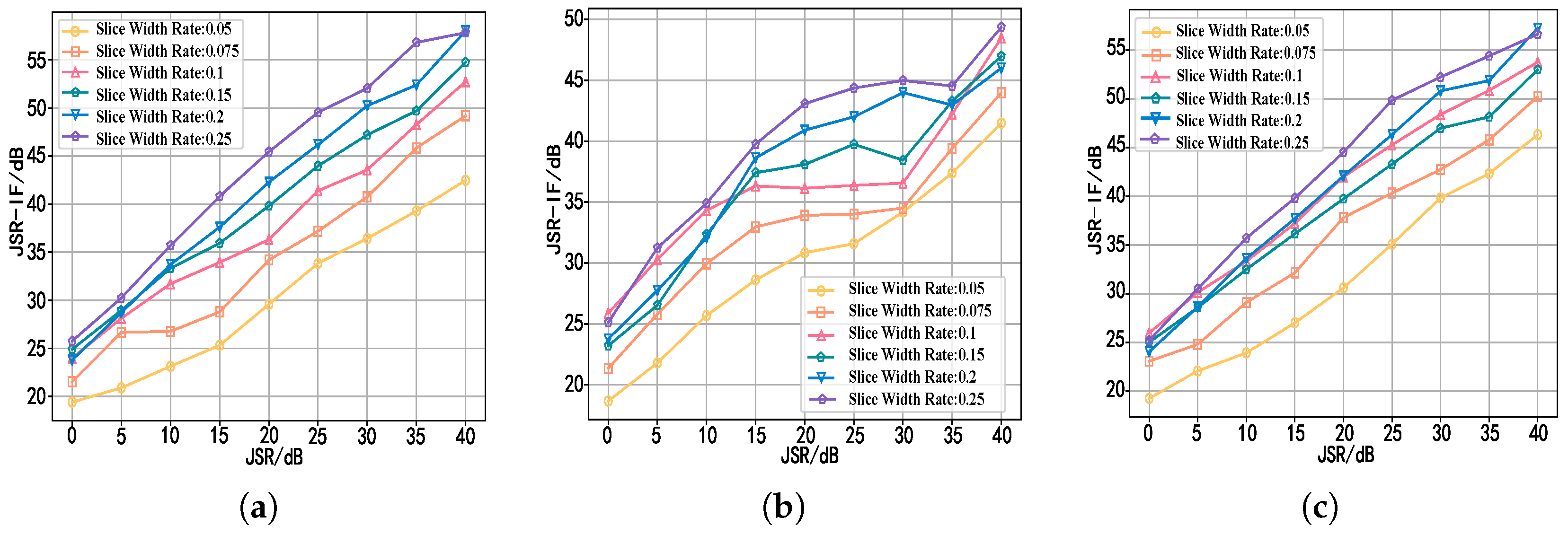
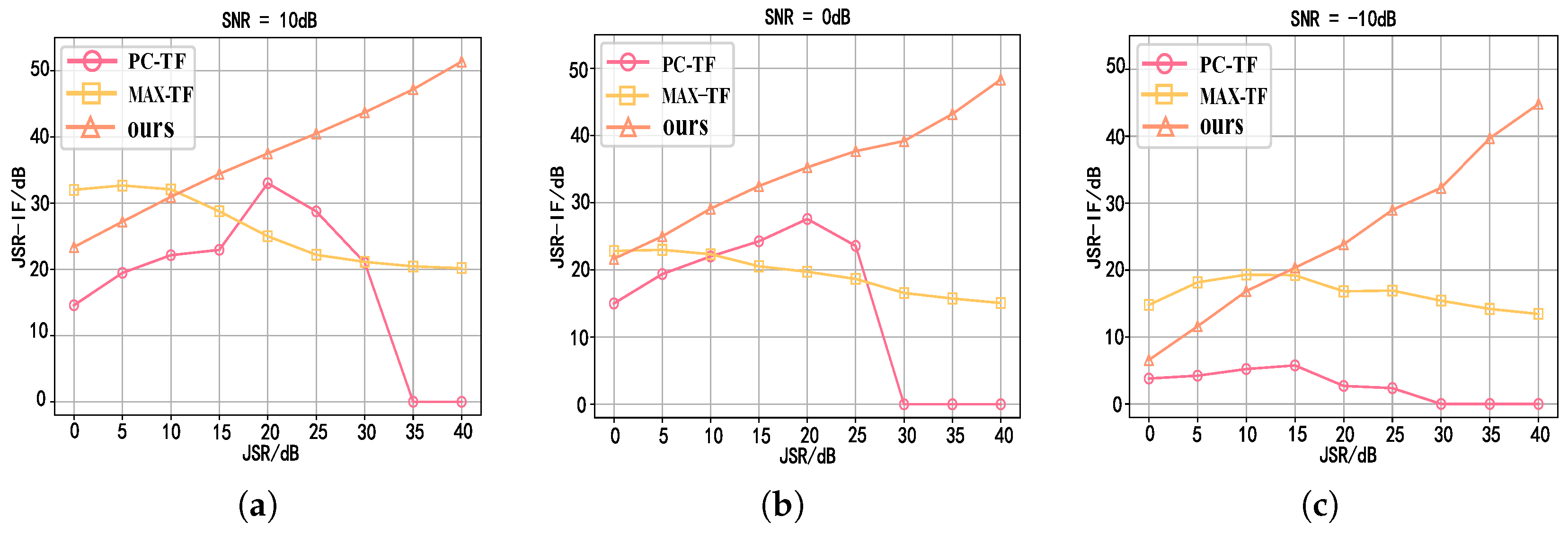
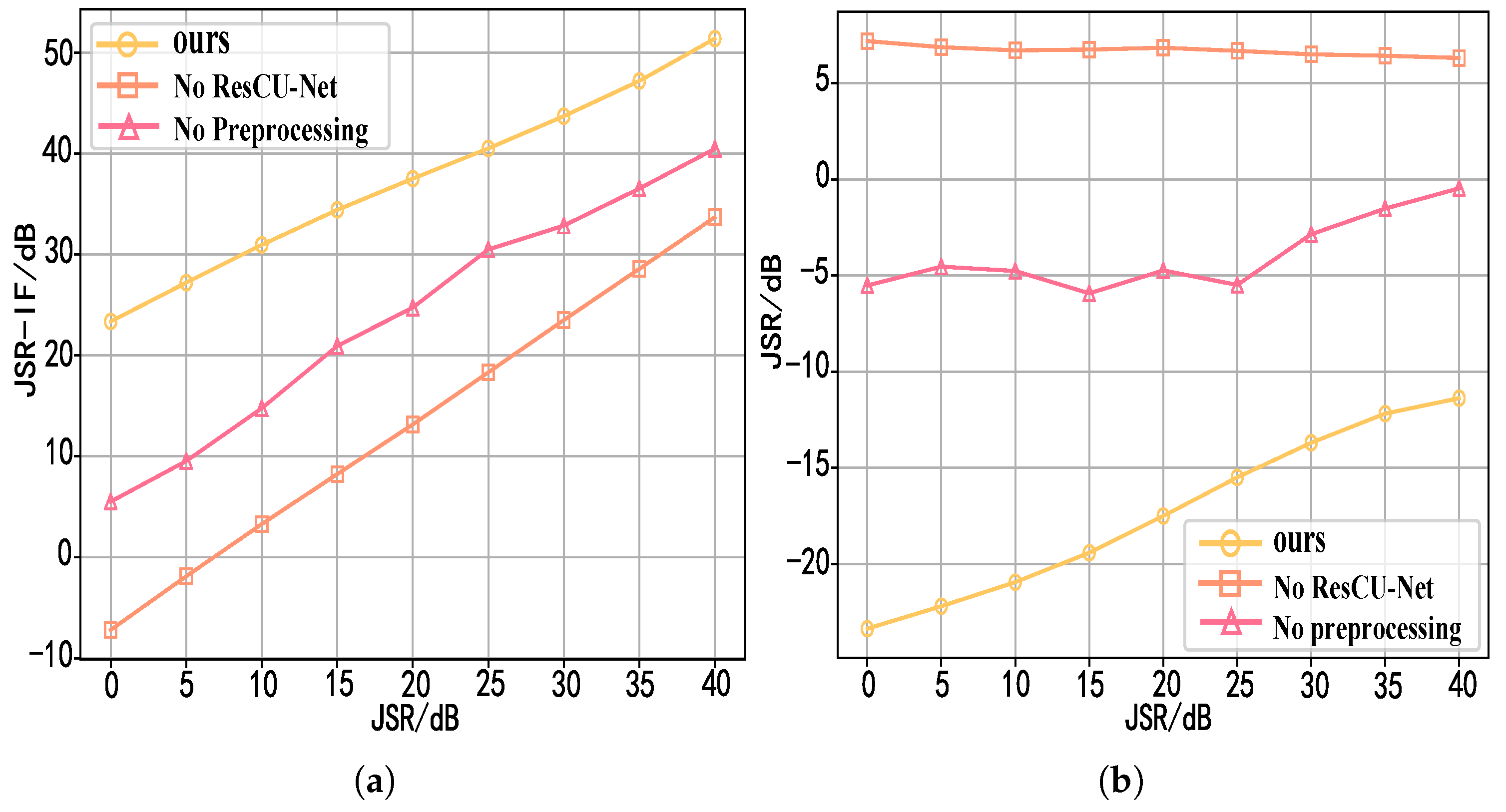
• Finally, in the experimental verification stage, the transmission signals with different slopes and bandwidths are used for testing, which verifies the signal recovery capability of the network under various ISRJs. We also demonstrate the effectiveness of each module through ablation experiments. They significantly improved the detection capabilities of radars.

The Section 2 introduces the signal model of the LFM radar and the working principle of the ISRJ. Section 3 details the proposed method, including each stage’s framework, preprocessing, network design, and training. Section 4 describes simulations used to compare the performance of the proposed method with two advanced filtering methods in the published literature. See Section 5 for conclusions.

2. Signal Model

The LFM signal is the common radar transmitting signal in radar. It has a large width and bandwidth and great target detection advantages. Therefore, this paper mainly studies the problem of ISRJ suppression under the LFM signal.

For the convenience of researching, assume that the true target used in this paper has just one scatter point. The normalized LFM signal emitted by the radar can be expressed as $s\left(t\right)$:

$$\begin{array}{c}\hfill s\left(t\right)=rect\left(\frac{t}{T}\right)e^{j2\pi \left(f_{c}t+\frac{K}{2}{t}^2\right)}\end{array}$$

(1)

$$\begin{array}{c}\hfill rect\left(\frac{t}{T}\right)=\left\{\begin{array}{c}1,\left|\frac{t}{T}\right|\le 1\hfill \\ 0,elsewise\hfill \end{array}\right.\end{array}$$

(2)

where $f_c$ denotes carrier frequency; $rect\left(\frac{t}{T}\right)$ is a rectangular window function with pulse width T; and $K=B/T$ is the frequency modulation rate, and B is bandwidth.

Assuming the target is a point target, the target echo signal is expressed as:

$$s_{tar}\left(t\right)=A_{tar}s\left(t-{\tau }_{tar}\right)$$

(3)

where $A_{tar}$ is a constant, representing the amplitude of the target signal; and ${\tau }_{tar}=2R_{tar}/T$ is the time delay from the jammer to radar, where $R_{tar}$ is the range of target and c denotes the speed of light.

ISRJ is formed by using DRFM to sample radar signals and then repeat them in sequence intermittently. Its principle is shown in Figure 1. The gray is the sampling time slice, and the blue is the forwarding time slice. According to different intermittent sampling methods, periodic sampling repeating jamming can be subdivided into jamming with direct repeater (ISDRJ), jamming with repetitive repeater (ISPRJ), and jamming with circular repeater (ISCRJ):

$$\begin{array}{cc}\hfill & J_{ISDRJ}\left(t\right)=\sum _{n=1}^{N}rect\left(\frac{t-\left(2n+1\right)T_s}{T_s}\right)s\left(t-T_s\right)\hfill \end{array}$$

(4)

$$\begin{array}{cc}\hfill & J_{ISPRJ}\left(t\right)=\underset{m=1}{\sum ^M}\sum _{n=1}^{N}rect\left(\frac{t-n{T}_u-m{T}_s}{T_s}\right)s\left(t-m{T}_s\right)\hfill \end{array}$$

(5)

$$\begin{array}{cc}\hfill & J_{ISCRJ}\left(t\right)=\underset{m=1}{\sum ^N}\sum _{n=1}^{N-m+1}rect\left(\frac{t-a_m{T}_s-b_n{T}_s}{T_s}\right)s\left(t-b_n{T}_s\right)\hfill \end{array}$$

(6)

where N is the number of slices, $T_s$ is slice width, M is the number of times each slice is repeated (retransmission times), and $T_u=\left(M+1\right)T_s$ is the interception time interval of two adjacent slices; $a_m{T}_s$ is the interception time of the mth slice, and $b_n{T}_s$ is the corresponding delay when the slice is repeated for the nth time. The calculation formulas are expressed below:

$$a_m=\frac{m\left(m+1\right)}{2}-1,b_n=\frac{n\left(n+1\right)}{2}+n-1$$

(7)

Under self-defense jamming, the jammer and the target are set at the same position and the same speed. Considering other noises, the final echo signal received by the radar can be expressed as:

$$x\left(t\right)=s_{tar}\left(t\right)+j\left(t\right)+n\left(t\right)$$

(8)

where $s_{tar}\left(t\right)$ is true target signal; $j\left(t\right)$ is jamming, as shown on Equations (4)–(6); and $n\left(t\right)$ is noise.

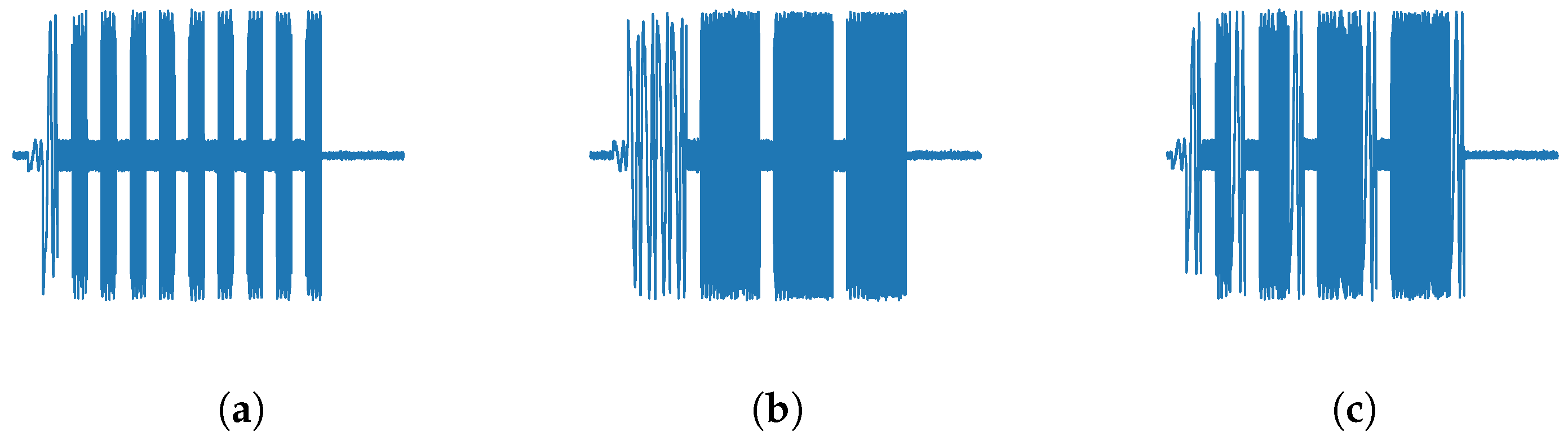
The time-domain signals of radar echo in the three jamming modes are shown in Figure 2.

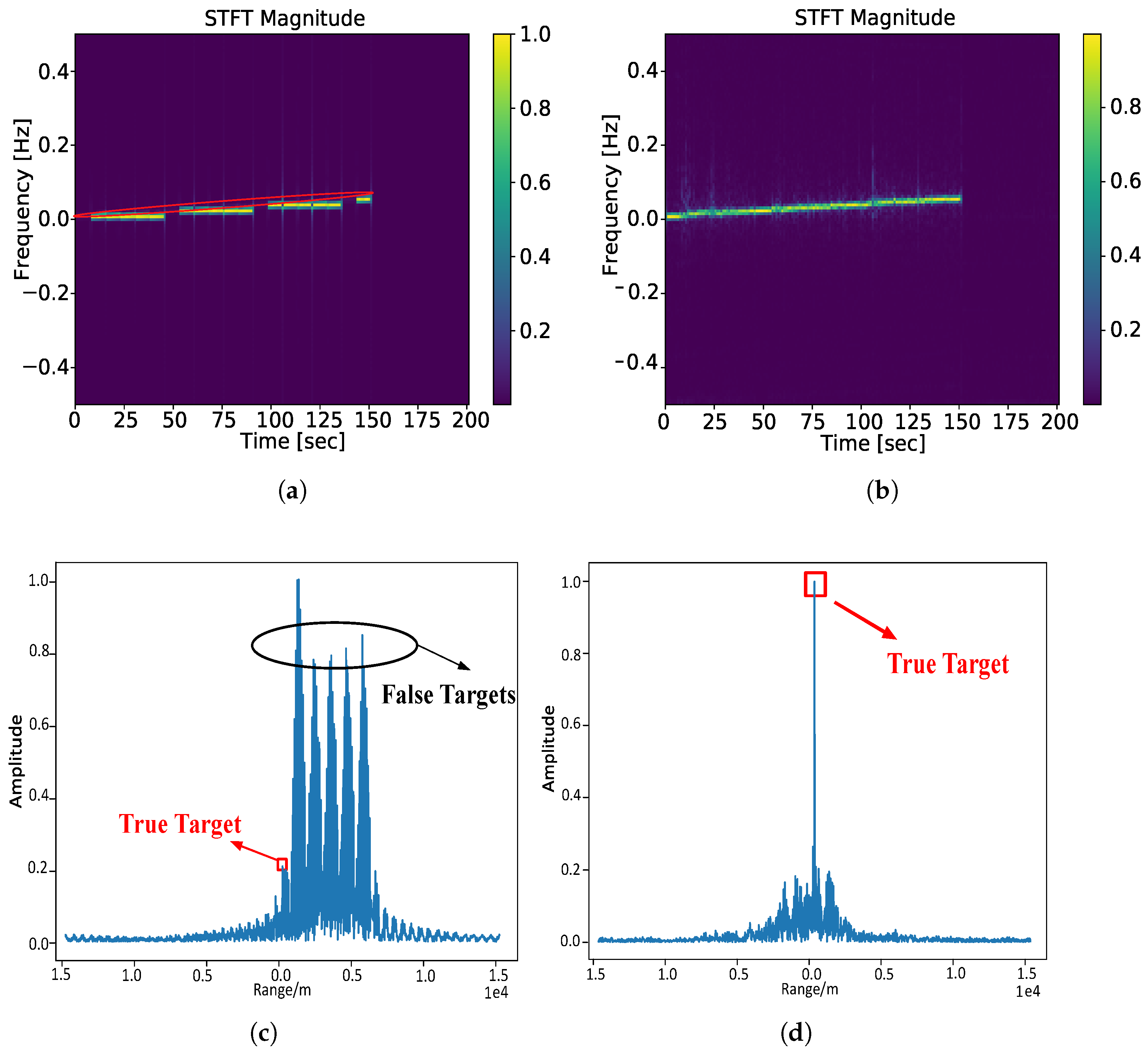
We take the short-time Fourier transform (STFT) of the radar echo $x\left(t\right)$ to obtain its time-frequency spectrum $\mathsf{\Omega }\left(t,f\right)$. The transformation formula is as in Equation (9).

$$\mathsf{\Omega }\left(t,f\right)=STFT\left\{x\left(t\right)\right\}=\underset{-\infty }{\overset{+\infty }{\int }}x\left(\tau \right)\omega \left(\tau -t\right)e^{-j2\pi ft}d\tau$$

(9)

The echo time-frequency amplitude spectra under three modes of ISRJ are shown in Figure 3.

In the time domain shown in Figure 2, the target and jamming signal overlap for a long time, so it is not easy to separate them directly. In the time-frequency spectrum shown in Figure 3, the long line segment corresponds to the true target echoes, and the discontinuous short line segment corresponds to the false target echoes. The target and jamming have relatively obvious length and continuity differences in the time-frequency amplitude spectra, so it is more conducive to realizing the separation of the target signal and jamming signal in the time-frequency domain.

3. Method

First, through the analysis of the jamming characteristics in Section 2, considering that the distribution of jamming and target on the time-frequency spectrum has obvious separable characteristics, we designed a UT-net to initially suppress the jamming on the time-frequency spectrum. The time-domain echo of the target can be obtained by ISTFT operation on the time-frequency spectrum after jamming suppression. However, the jamming suppression processing on the time-frequency spectrum will ignore the phase information of the true echo, so the signal recovered by ISTFT is only a preliminary reconstruction of the echo signal of the target. Therefore, in order to further eliminate the jamming-signal component and restore the detailed information of the target echo, we designed a ResCU-net to further suppress the jamming in the signal time domain. In this multi-stage method, the characteristic information of the target echo is gradually recovered from two different perspectives: the time-frequency domain and the time domain. On the one hand, it has a better jamming suppression effect than the end-to-end network structure; on the other hand, it also increases the interpretability of the model function.

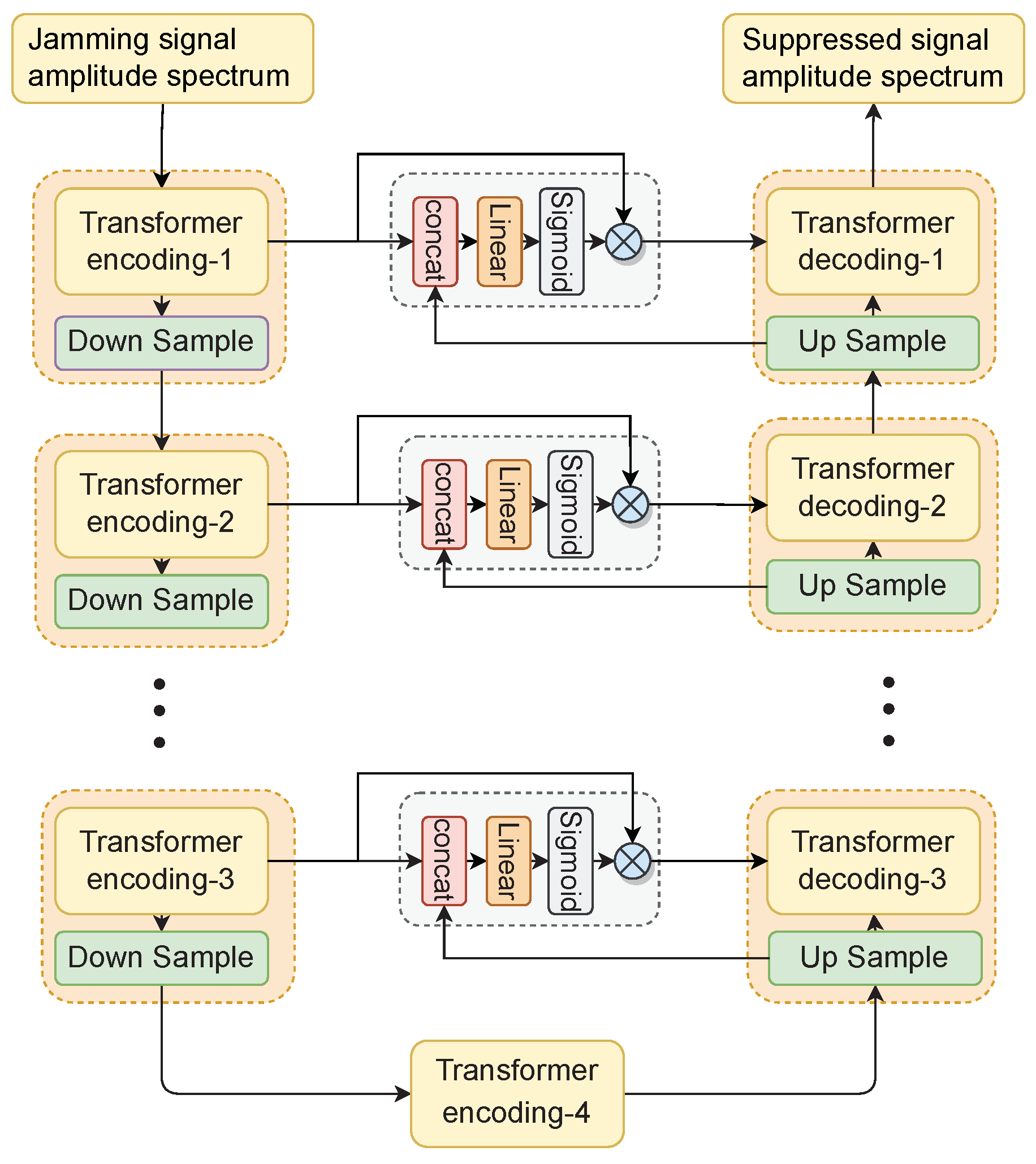
Accordingly, this paper proposes a deep-learning model based on multi-stages and multi-domains (MSMD), which can suppress the jamming signal components in the radar echo and then reconstruct the true echo of the target. The model structure of MSMD-net is shown in Figure 4, and its processing flow is mainly divided into three stages:

The first stage is the signal preprocessing. The primary purpose is to obtain the normalized amplitude spectrum ${\mathsf{\Omega }}_{in}$ and phase spectrum $\mathsf{\Phi }$ from the input signal $x\left(t\right)$ in the time-frequency domain. Among them, to improve the network’s robustness and enhance its ability to perceive real targets in the case of high JSR, we propose the shape-matching operator to obtain the true target signal strength. Then, we limit and filter the amplitude spectrum ${\mathsf{\Omega }}_{in}$ to lower the jamming signal strength and reduce the JSR.

In the second stage, the jamming on the time-frequency domain amplitude spectrum is suppressed through UT-Net. UT-net is composed of a U-Net structure with transformer modules, and its input is the normalized amplitude spectrum ${\mathsf{\Omega }}_{limit}$, which can be obtained from limiting filtering. Its output is the amplitude spectrum ${\mathsf{\Omega }}_{out}$ after suppression. Combining it with the original phase map $\mathsf{\Phi }$ for inverse short time Fourier transform (iSTFT), the echo signal $y_{origin}$ can be initially recovered:

$$y_{origin}=iSTFT\left({\mathsf{\Omega }}_{out}{e}^{j\mathsf{\Phi }}\right)$$

(10)

In the third stage, we used the ResCU-net network to repair the details in the signal time domain locally. ResCU-net is composed of Complex-1D-CNN (one-dimensional complex convolution network) combined with the U-Net network. Its input is the preliminary reconstruction signal $y_{origin}$ of the second stage, and the output is the final output signal $y_{output}$.

3.1. Preprocessing

In the preprocessing stage, we first needed to carry out complex mixing processing on the signal, and the signal carrier frequency was down converted to zero frequency. Then, we performed short-time Fourier transform on the transmitted signal $s\left(t\right)$ and the received signal $x\left(t\right)$ to obtain their time-frequency spectra: ${\mathsf{\Omega }}_s$ and ${\mathsf{\Omega }}_{in}$. A 3 dB threshold was used to binarize ${\mathsf{\Omega }}_s$ to obtain a binarized time-frequency spectrum ${\mathsf{\Omega }}_{bs}$. A shape-matching operator ${Filter}_{LFM}$ was constructed with the binarized time-frequency spectrum of the transmitted signal as auxiliary information. Secondly, we used the matching operator to convolve the time-frequency spectrum ${\mathsf{\Omega }}_{in}$ with a sliding window to find a suitable limiting threshold $thresh$. Finally, we performed limiting filtering on ${\mathsf{\Omega }}_{in}$ of the received signal and obtained the output of the preprocessing stage: ${\mathsf{\Omega }}_{limit}$.

Algorithm 1 shows the process of building a shape-matching operator using the transmitted signal. We used the −3 dB threshold to binarize the time-frequency spectrum ${\mathsf{\Omega }}_s$. Then, the frequency energy width $T_w$, time energy width $F_w$, and the transmit signal $s\left(t\right)$ location in the binarized spectrum ${\mathsf{\Omega }}_{bs}$ were calculated. Finally, we constructed a shape-matching operator $Filte{r}_{LFM}\in R^{T_w\times F_w}$.

Algorithm 2 is used to judge whether there is a transmit signal $s\left(t\right)$ on the binary spectrum ${\mathsf{\Omega }}_{bin}$. The matching operator ${Filter}_{LFM}$ slides convolution calculates the matching degree $\rho$ on ${\mathsf{\Omega }}_{bin}$. When there is a matching degree greater than 0.95, it means that the transmit signal exists.

Algorithm 1: Built shape-matching Operator

Input: Transmit signal: $s\left(t\right)$     1: Time-Frequency domain amplitude spectrum with STFT: ${\mathsf{\Omega }}_s\left(t,f\right)\leftarrow STFT\left(s\left(t\right)\right)$     2: 3dB energy threshold: $thresh\leftarrow 0.707\ast Max\left({\mathsf{\Omega }}_s\right)$     3: Binary spectrum: ${\mathsf{\Omega }}_{bs}\left(t,f\right)=\{\begin{array}{cc}1,\hfill & if{\mathsf{\Omega }}_s\left(t,f\right)\le thresh\hfill \\ 0,\hfill & otherwise\hfill \end{array}$     4: Energy peak at each moment: $T_{max}\left(t\right)=\underset{f=1:end}{max}{\mathsf{\Omega }}_{bt}\left(t,f\right)$     5: Energy peak at each frequency band: $F_{max}\left(t\right)=\underset{t=1:end}{max}{\mathsf{\Omega }}_{bt}\left(t,f\right)$     6: Frequency energy-width: $T_w\leftarrow Sum\left(T_{max}\right)$     7: Time energy-width: $F_w\leftarrow Sum\left(F_{max}\right)$     8: ${Filter}_{LFM}\leftarrow {\mathsf{\Omega }}_{bs}[0:0+F_w,0:T_w]$   Output: Shape-matching Filtering Operator: ${Filter}_{LFM}$

Algorithm 2: Compare-Energe

Input: Binary spectrum of Echo signal: ${\mathsf{\Omega }}_{bin}$     1: Energe: $Energe\leftarrow Sum\left({Filter}_{LFM}\right)$     2: Matching degree threshold: $thre\leftarrow 0.95$     3: Length and width of Filter: $h,w$     4: Fill zeros with w width on the left and right sides of ${\mathsf{\Omega }}_{bin}$     5: $x\leftarrow w/2$     6: $Exist\leftarrow True$     7: while$x\ne Width\left({\mathsf{\Omega }}_{bin}\right)-w/2$ do     8:     Matching Energe ${Energe}_m$:     $Sum\left({Filter}_{LFM}\ast {\mathsf{\Omega }}_{bin}\left[h,x-w/2:x+w/2+1\right]\right)$     9:     Matching degree $\rho \leftarrow {Energe}_m/Energe$     10:   if $\rho \ge thre$ then     11:          $Exist\leftarrow True$     12:         return $Exist$     13:   end if     14:   $x\leftarrow x+1$     15: end while     16: $Exist\leftarrow Flase$     17: return $Exist$

Algorithm 3 shows the main process of limiting filtering. We first used 3 dB to initialize the threshold $thresh$ to obtain the binarized spectrum of the received signal. On the condition that the matching degree $\rho$ is greater than 0.95, $thresh$ was iteratively updated until the condition is satisfied. Finally, the time-frequency spectrum was limiting filtered by the obtained threshold $thresh$.   

Algorithm 3: Limiting-filtering

Input: Transmit signal: $s\left(t\right)$, Echo signal: $x\left(t\right)$     1: Build Shape-matching Filtering Operator: ${Filter}_{LFM}$     2: Time-Frequency domain amplitude spectrum with STFT: ${\mathsf{\Omega }}_{in}\left(t,f\right)\leftarrow STFT\left(x\left(t\right)\right)$     3: 3dB energy threshold: $thresh\leftarrow 0.707\ast Max\left({\mathsf{\Omega }}_{in}\right)$     4: Binary spectrum: ${\mathsf{\Omega }}_{bin}\left(t,f\right)=\{\begin{array}{c}1,if{\mathsf{\Omega }}_{in}\left(t,f\right)\le thresh\hfill \\ 0,otherwise\hfill \end{array}$     5: while Compare-Energe $\left({\mathsf{\Omega }}_{bin}\right)$ do     6:      $thresh\leftarrow 0.707\ast thresh$     7:     ${\mathsf{\Omega }}_{bin}\left(t,f\right)=\{\begin{array}{c}1,if{\mathsf{\Omega }}_{in}\left(t,f\right)\le thresh\hfill \\ 0,otherwise\hfill \end{array}$     8: end while     9: ${\mathsf{\Omega }}_{bin}\left(t,f\right)=\{\begin{array}{c}1,if{\mathsf{\Omega }}_{in}\left(t,f\right)\le thresh/0.5\hfill \\ 0,otherwise\hfill \end{array}$     10: Limiting-Filtering ${\mathsf{\Omega }}_{limit}$: ${\mathsf{\Omega }}_{bin}\ast {\mathsf{\Omega }}_{in}+\left(1-{\mathsf{\Omega }}_{bin}\right)\ast {\mathsf{\Omega }}_{in}/\left(thresh/0.5\right)$   Output: ${\mathsf{\Omega }}_{limit}$

3.2. UT Network

In the analysis in Section 2, we concluded that the interrupted sampling mechanism of the DRFM jammer will cause the target echo to show a continuous long sloping line on the time-frequency spectrum, while the jamming will show interrupted repeated short sloping lines. Therefore, we first considered using this feature to identify and filter out jamming on the time-frequency spectrum. The traditional methods of jamming suppression are mainly to determine the discontinuous area and repetitive area of the signal by setting the threshold, so as to realize the distinction and suppression of the target and the jamming. However, these methods mostly depend on the experience of experts, and it is easy to fail when the jamming parameters, JSR, and SNR change. Therefore, we designed a UT-net model to automatically realize jamming suppression and target signal restoration on the time-frequency spectrum. The model adopts the U-net architecture with the transformer structure.

U-net uses a self-encoding structure to map signals from high-dimensional signal space to low-dimensional feature space, and then restore from low-dimensional features to high-dimensional signals. This low-dimensional mapping process is the process of extracting the key information of the target and filtering out the jamming information. In the process of restoring from low-dimension to high-dimension, U-net adopts a skip connection mechanism to realize the fusion of multi-scale features, and then better complete signal recovery. Therefore, we used U-net as the basic network architecture to achieve jamming suppression and target echo reconstruction.

However, in the original U-net network, since it adopts the CNN layer in both the encoding layer and the decoding layer, it has a strong ability to capture the local features of the signal, but it is difficult to pay attention to the global shape features of the signal. For interrupted sampling jamming, the jamming is a local copy of the signal. If it only focuses on the local features of the jamming and the target, there will be great similarity between them, which is not conducive to separation. While the true signal is continuous in time, the jamming is discontinuous, so their correlation over the entire time period will be different. In order to enable the network to better pay attention to this relevant feature of the signal globally, we replace the CNN layer in the U-net with the encoder and decoder module of the transformer. The transformer has a stronger modeling ability than CNN, and the self-attention module it contains can model the relationship between all elements well. In addition, the transformer module also uses cross-attention on the decoding layer. Compared with the linear combination in the splicing operation, cross-attention can introduce more nonlinear information, better fuse the lower-layer semantics and cross-layer semantic information, and improve the UT-net network’s ability to reconstruct the target signal.

Therefore, the UT-net with the transformer module added can pay attention to the characteristics of the target signal and the jamming signal at different levels on the time-frequency spectrum, so as to suppress the jamming signal and reconstruct the target signal, accordingly.

The entire process of the UT-net is U-shaped. In Figure 5, the left part is the encoding—downsampling process, the right part is the decoding—upsampling process and the area in the middle is the skip connection of the feature map. U-net took n maxpool down-sampling layers. After each sampling, the transformer encoding layer extracts information to obtain the feature map. U-net also took n up-sampling layers, which were used to reconstruct the input pixel size. Then, it will go through the transformer decoding layer, which can fix spectrum details. They are shown in Equations (11) and (12):

$$\begin{array}{cc}\hfill & {{\mathsf{\Omega }}^n}_{down}=MaxPool\left(En{c}_n\left({{\mathsf{\Omega }}^{n-1}}_{down}\right)\right)\in C^{F\times \frac{T}{2n}}\hfill \end{array}$$

(11)

$$\begin{array}{c}\hfill \begin{array}{c}\hfill {{\mathsf{\Omega }}^{n-1}}_{up}=De{c}_n\left(Skip\left(Up\left({{\mathsf{\Omega }}^n}_{up}\right),De{c}_{n+1}\left({{\mathsf{\Omega }}^{n-1}}_{down}\right)\right),Up\left({{\mathsf{\Omega }}^n}_{up}\right)\right)\end{array}\end{array}$$

(12)

where ${{\mathsf{\Omega }}^n}_{down}$ is the output of the nth down-sample layer, $MaxPool$() is the function of the nth max pooling layer, ${{\mathsf{\Omega }}^{n-1}}_{up}$() is the output of the nth decoding layer, ${{\mathsf{\Omega }}^{n-1}}_{up}\in R^{F\times \frac{T}{2\left(n-1\right)}}$, $Up$() is the function of the nth up-sampling layer, $Skip$() is the function of the skip-connection layer. $En{c}_n$ represents the nth encoding layer, $De{c}_n$ represents the nth decoding layer.

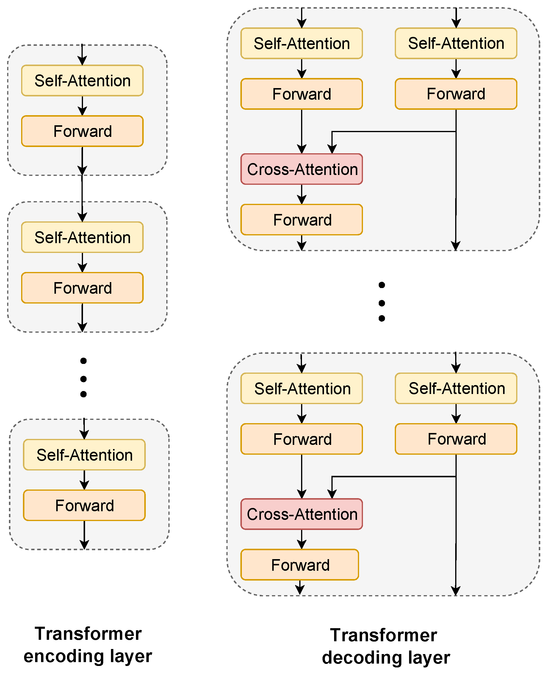
Figure 6 shows the internal structure of the transformer encoding layer and decoding layer. The function of the encoding layer is to extract signal features. In addition, each encoding layer, in Figure 5, can be composed of multiple encoders with the same structure cascaded. The input to the encoder is normalized magnitude spectrum ${\mathsf{\Omega }}_{limit}$ or downsampled ${{\mathsf{\Omega }}^{n-1}}_{down}$. The internal structure of each encoder consists of a self-attention mechanism layer and a forward propagation layer. The decoding layer is also composed of multiple cascaded decoders; its input is the upsampled ${{\mathsf{\Omega }}^n}_{up}$ and skip-connection layer input. The overall structure of each decoder (see Figure 5) consists of two self-attention layers and one cross-attention layer. The design of the two self-attention layers mainly balances the input dimension. It ensures that the feature dimension space of the two inputs is the same when calculating the cross attention.

The most critical part of the U-net is the skip connection of the middle area. However, considering that the jamming amplitude is greater than the signal amplitude during the anti-jamming process of the radar signal, there may be still residual jamming in the coding stage. The jamming will be re-transmitted to the subsequent layers by the skip connection, which is not conducive to the decoding layers’ recovery of the signal amplitude.

Therefore, the network should selectively return the information of the encoding layer in the skip connection to reduce the jamming components entering the decoding layer. This paper refers to the design of the forget gate in LSTM [20]. It uses the full-connect layer and the sigmoid function to design and generate the forgetting matrix so that the skip-connection layer can selectively input the information of the encoding layer into the subsequent decoding layer.

$$\begin{array}{cc}\hfill & Skipnet\left(Up\left({{\mathsf{\Omega }}^n}_{up}\right),{{\mathsf{\Omega }}^{n-1}}_{down}\right)=\hfill \\ \hfill & {{\mathsf{\Omega }}^{n-1}}_{down}\ast Sigmoid\left(Linear\left(Up\left({{\mathsf{\Omega }}^n}_{up}\right),{{\mathsf{\Omega }}^{n-1}}_{down}\right)\right)\hfill \end{array}$$

(13)

where $Sigmoid$() is sigmoid function, and $Linear$() is the full-connect layer.

3.3. ResCU Network

We use the time-frequency amplitude spectrum obtained in Section 3.3 and the original phase spectrum of the received signal to initially recover the target echo signal. Considering that the original phase spectrum is also affected by jamming and noise, the recovered signal still has some jamming. To this end, we continue to use the U-net architecture in the signal time domain to further suppress the jamming component and restore the local details of the signal. Although the transformer module in UT-net can extract global information, it has insufficient ability to obtain local details. Therefore, at this stage, using a CNN layer that can pay more attention to local details and has lower complexity is a better choice. At the same time, considering that the radar echo signal is a complex signal, in order to combine the real-part and imaginary-part features of the signal, at this stage, we chose the complex residual convolution module to replace the transformer to form the ResCU-net structure. Compared with the transformer module in UT-net, the complex residual convolution module of ResCU-net can better pay attention to the local details of the signal in the time domain and improve the recovery accuracy of the true echo. In addition, its residual structure also ensures that it can form a deeper network structure and improve the learning ability of the network.

The overall ResCU-net model structure is similar to the structure described in UT-net. The main difference is that the encoder and decoder of the transformer are replaced with a Complex-1D-CNN [30], and the pooling layer is no longer used. We chose to use the method of expanding the convolution-kernel step size to achieve dimensionality reduction. The structure of each layer is composed of a residual convolution layer, activation function layer, and batch normalization layer. The number of channels is doubled after each convolution. The upsampling process is the same, but the number of channels is gradually decreased. The skip-connection layer between them is changed to splicing in the channel dimension of the up-sampled signal and then input to the complex-valued convolutional network together.

3.4. Loss Function

The loss value is calculated using the model output signal $y_{output}$ and target signal $y_{target}$. The loss function is set as the mean square error function in the time domain ($L_T$ in Equation (14)), time-frequency domain ($L_{T-F}$ in Equation (15)), and Hilbert domain ($L_{H-T}$ in Equation (16)):

$$\begin{array}{cc}\hfill L_T& =\sqrt{\frac{1}{N}\underset{i=1}{\sum ^N}{\left({y_{output}}_i-{y_{target}}_i\right)}^2}\hfill \end{array}$$

(14)

$$\begin{array}{cc}\hfill L_{T-F}& =\sqrt{\frac{1}{HW}\underset{i=1}{\sum ^H}\underset{j=1}{\sum ^W}{\left({{\mathsf{\Omega }}_{final}}_{ij}-{{\mathsf{\Omega }}_{target}}_{ij}\right)}^2}\hfill \end{array}$$

(15)

$$\begin{array}{cc}\hfill L_{H-T}& =\sqrt{\frac{1}{N}\underset{i=1}{\sum ^N}{\left(Hilbert\left({y_{output}}_i\right)-Hilbert\left({y_{target}}_i\right)\right)}^2}\hfill \end{array}$$

(16)

where N is the length of $y_{output}$, ${\mathsf{\Omega }}_{final}$, and ${\mathsf{\Omega }}_{target}$ are the time-frequency domain amplitude maps obtained by short-time Fourier transform of $y_{output}$ and $y_{target}$, respectively. ${\mathsf{\Omega }}_{final},{\mathsf{\Omega }}_{target}\in C^{H\times W}$. $Hilbert$() is the Hilbert transform.

The mean square error function on the time domain ensures the consistency of the signal’s energy in the time domain. The mean square error function on the Hilbert domain improves the accuracy of the pulse signal on the rising and falling edges. The square error function ensures the linear representation of the signal on the time-frequency diagram. It provides that the waveform of the recovered signal is consistent with the transmitted signal, which is convenient for subsequent pulse compression processing.

$$L_{UT}=\sqrt{\frac{1}{HW}\underset{i=1}{\sum ^H}\underset{j=1}{\sum ^W}{\left({{\mathsf{\Omega }}_{out}}_{ij}-{{\mathsf{\Omega }}_{target}}_{ij}\right)}^2}$$

(17)

As MSMD-net is a multi-stage network, making each stage’s network model play a corresponding suppression effect is necessary. We designed a loss function for the output of the intermediate stage to calculate the mean square error of the time-frequency amplitude spectrum of the UT-Net network output ${\mathsf{\Omega }}_{out}$ and the target signal ${\mathsf{\Omega }}_{target}$, in Equation (17). It ensures that the UT-net can converge in the direction we expect during training, reducing the difficulty of network training. Finally, the loss function of the whole network can be expressed using Equation (18).

$$Loss=L_T+L_{T-F}+L_{H-T}+L_{UT}$$

(18)

In addition, during the training process, unlimited random training will lead to a low probability of some extreme hard cases; it will be difficult for the network to learn their characteristics. In the article by He et al. [29], a new focal loss is proposed to solve the learning problem of hard and easy samples in the image-classification problem. The idea is that, for inaccurately classified samples, the loss remains unchanged. For accurately classified samples, the loss is reduced. Overall, it is equivalent to increasing the weight of hard samples in the loss function. With this idea in mind, this paper proposes focal loss based on regression problems, which is different from the idea of judging difficult samples by relying on probability values in classification problems. We focus more on the regression differences of different samples in a miniBatch. That is, according to the Loss size between each sample, the difficult and easy samples are distinguished, the learning rate of the difficult samples is increased, and the network update direction is more inclined to the direction of the difficult samples. See the formula for the specific implementation.

$$Batch\_Loss=\underset{i=1}{\sum ^N}\frac{e^{Los{s}_i}}{\sum e^{Los{s}_i}}Los{s}_i$$

(19)

where $Los{s}_i$ is the loss obtained by each sample in a batch. $Batch\_Loss$ is the loss to be updated in this batch.

4. Experiments

To verify the effectiveness of the proposed algorithm, we designed a series of Monte Carlo experiments. The jamming suppression ability of the network model under different jamming strategies was analyzed from the perspective of jamming-suppression capability and target-detection capability.

4.1. Simulations

In the model training, we adopted the infinite training method, which means we randomly selected the parameters of radar transmitter, receiver, target, ISRJer, and noise environment, and used the simulation model in Section 2 to generate echo signal for training until the network converged. The specific parameter selection interval is shown in

Table 1. Training samples generating parameters’ setting.

The parameters of radar transmitter
Carrier frequency ($f_c$)	100 MHz
Sampling frequency ($f_c$)	150 MHz
Radar signal cycle ($T_r$)	150 $\mathsf{\mu }$s
Pulse width (T)	[50, 150] $\mathsf{\mu }$s
Pulse bandwidth (B)	[5, 50] MHz
The parameters of target
Max range ($R_{max}$)	$[5,10]$ km
Target range ($R_{tar}$)	$[0,R_{max}]$ km
The parameters Of ISRJer
ISRJer working mode	ISDRJ, ISPRJ, ISCRJ
ISRJ slice width ratios	[0.02, 0.3]
SNR ($SNR$)	[−10, 10] dB
JSR ($JSR$)	[0, 50] dB

, and the selection of parameters follows a uniform distribution.

In the model testing, in order to ensure the accuracy of the test as much as possible, we chose a wider variety of slice width rates (the width ratio of the jamming slice and the signal pulse), JSR, and SNR to generate test signals on the basis of Table 1. Under each slice width rate, SNR, and JSR, 50 sets of echo signals at different target positions will be generated. There are a total of 7 slice width rates, 4 SNRs, and 9 JSRs in the three ISRJer operating modes. Eventually, 37,800 echo data will be generated for Monte Carlo testing.

In addition, the Adam optimizer was utilized in the MSMD-net method. The learning rate was set to $1\times {10}^{-4}$. The computer performed all simulations with Intel Core i7-11700 CPU@2.50 GHz and NVIDIA GeForce RTX 3060.

4.2. Method Performance

The jamming suppression and real target-retaining ability of the three methods are measured by the metric of jamming-to-signal ratio improvement factor (JSR-IF). After matched filtering the echo, the range profile was obtained. It can be expressed as $s_p\left(t\right)$. Then, the JSR (jamming-to-signal ratio) after pulse compression is defined as:

$$\mathrm{JSR}=20\mathrm{lo}{\mathrm{g}}_{10}\left(\frac{a_{jam}}{a_{tar}}\right)$$

(20)

where $a_{tar}$ is the maximum target amplitude after echo pulse compression; and $a_{jam}$ is the maximum amplitude of jamming target after pulse compression. Then, JSR-IF can be expressed as:

$$\mathrm{JSR}-\mathrm{IF}={JSR}_{unfiltered}-{JSR}_{filtered}$$

(21)

where ${JSR}_{filtered}$ is the JSR of pulse compression after jamming suppression; and ${JSR}_{unfiltered}$ is the result of original pulse compression without jamming suppression.

In addition, the detection performance of radar can be demonstrated by detection rate ($P_d$) and accurate detection rate ($P_{acc}$). The detection rate is the rate of radar-detecting targets in PC results in $s_p\left(t\right)$ using CFAR detectors, which is defined as follows:

$$P_d=N_t/S_t$$

(22)

where $N_t$ is the number of correctly detected targets in true targets, and $S_t$ is the total number of true targets that exist in the range profile after pulse compression.

The accurate detection rate $P_{acc}$ is the rate of the samples in which the radar only detects all real targets, and no false targets were detected in all test samples. It is defined as follows:

$$P_{acc}=N_{acc}/S_{acc}$$

(23)

where $N_{acc}$ is the number of samples that only detected all real targets and no false targets were detected. $S_{acc}$ is the number of test samples.

4.3. Result and Analysis

We used the well-trained MSMD-Net to suppress the generated test data. A sample simulation result is displayed in Figure 7. Figure 7a,c shows the time-frequency domain characteristics of the original signal and the pulse compression results before network suppression. In the time-frequency domain, we can see that the jamming signal completely masks the target signal in the red circle. Similar results are also reflected in the pulse compression profile. The true target peaks out of the red frame are surrounded by dense false target groups, hindering subsequent target detection. The suppression results of the original signal by MSMD-Net are shown in Figure 7b,d. From the results in Figure 7b, it can be seen that the MSMD-net suppresses the jamming signal well in the time-frequency domain, highlighting the chirp characteristic of the clean echo. This suppression effect is also reflected in the one-dimensional range profile after pulse compression. As can be seen in Figure 7d, the false target peaks are completely suppressed, while the true target peaks are preserved.

4.3.1. Jamming Suppression

Figure 8 shows the suppression effect of MSMD-net in different ISRJer Modes, slice width ratios, and JSRs. From Figure 8, we can see some facts:

(a)

JSR-IF of MSMD-net under three disturbances increases with increasing JSR. In JSR ranging from 5 to 50 dB with an interval of 5 dB, the JSR-IF of MSMD-net is, on average, more than 10 dB higher than that of JSR, proving that the method can effectively suppress jamming under each JSR. In addition, comparing the three pictures, it can be seen that the rising curves of JSR-IF of ISDRJ and ISCRJ are similar, and the fluctuation in ISPRJ is larger. The reason is that the jamming effects of ISDRJ and ISCRJ are relatively single, and ISPRJ is also affected by the number of the repeated jamming slice, and the jamming effects will be more diverse.

(b)

We observed the jamming-suppression effect of MSMD net on different slice width ratios under three interference forms. It can be seen that, with the decrease in the slice width ratio, the suppression effect of the network will gradually deteriorate. The reason is that the reduction in the slice width ratio will lead to the reduction in the length of the jamming slice, the increase in the sampling times of the DRFM jammer, and the wider distribution of the jamming signal in the spectrum. As a result, the correlation between the jamming signal and the target signal is stronger, and the generated false target is closer to the real target position, bringing more difficulty to jamming suppression. Nevertheless, MSMD-net still maintains sufficient JSR-IF under a small slice width ratio, ensuring the suppression ability of the network.

4.3.2. Algorithm Comparison

The proposed MSMD-net method was compared with the two most advanced filtering methods, which were referred to as PC-TF [30] and max-TF [16] methods in this paper. Our method and the two competitors were tested under different ISRJer, SNR, and JSR conditions. The result is shown in

Table 2. Comparison of suppression and detection performance of different methods under JSR = 25 dB and SNR = 0 dB.

Method	${\mathit{P}}_{\mathit{d}}$		${\mathit{P}}_{\mathbf{acc}}$
	Before Suppress	After Suppress	Before Suppress	After Suppress
PC-TF	0.63	0.83	0.0	0.01
max-TF	0.63	0.85	0.0	0.05
Ours	0.63	0.99	0.0	0.85

and Figure 9.

In Table 2, we show the detection performance of different methods under JSR = 20 dB & SNR = 0 dB. Compared with the detection rate, the accurate detection rates of PC-TF and max-TF methods have dropped significantly, which are the same as the accurate detection rates before interference suppression. Moreover, the accuracy detection rate of our method drops by a small margin. This shows that the other two methods can only improve the recognition ability of radar for real targets but cannot suppress false targets. Furthermore, our method can suppress false targets to a great extent and highlight real targets. It greatly reduces the burden of follow-up work.

In Figure 9, we calculate the JSR-IF curves of the three jamming-suppression methods as a function of JSR under three signal-to-noise ratios in detail. As shown in Figure 9, we can see that:

(a)

Except when 0 dB < JSR < 10 dB, the JSR-IF of our method is slightly lower than the max-TF method; in other various SNR and JSR cases, the JSR-IF of MSMD-net is significantly higher than the other two methods. Especially when the JSR > 25 dB, the JSR-IF of the other two methods decreases, and the JSR-IF is much smaller than the JSR of the jamming signal. However, the JSR-IF of our method still increases with the increase in JSR and is basically not affected by JSR.

(b)

When SNR = 0 to 10 dB and JSR = 20 to 30 dB, the suppression effect of the PC-TF method is slightly better than that of the max-TF method, but in other cases, the suppression ability is lower than the max-TF method.

(c)

Comparing the three pictures, it can be seen that, with the increase in SNR, under the same JSR, the suppression effect of the PC-TF algorithm decreases the fastest and can only maintain a certain suppression effect when the SNR = 0 to 10 dB. The suppression effect of Max-Tf method decreases slowly. When the SNR decreases by 10 dB, its JSR-IF also decreases by about 10 dB on average. However, our method is basically not affected by the change in SNR when SNR $>0$ dB. The suppression ability begins to weaken only when the SNR < 0 dB. When the SNR drops from 0 dB to −10 dB, the JSR-IF of our method also drops by about 10 dB on average.

4.3.3. Ablation Experiments

This paper mainly conducted ablation experiments on the proposed preprocessing module and ResCU-Net to verify the necessity of using a multi-stage network to achieve jamming suppression. The experimental results are shown in Figure 10. It can be seen from the above experiments that:

(a)

The model without the ResCU-net (No-ResCU net) has the worst jamming-suppression ability. Its effect is significantly lower than the MSMD-net and the network without preprocessing (No-preprocess net). From Figure 10a, it can be seen that the JSR-IF without the ResCU-net increases steadily with the increase in the JSR, indicating that the pure UT-net has a certain inhibitory effect. However, in Figure 10b, its recovered signal JSR is still greater than zero, indicating that the strength of the jamming signal is still greater than that of the target signal. This shows that only using the combined method of the amplitude map and the original phase map for signal recovery causes a large loss of accuracy. After adding the ResCU-net, the suppression effect of the model under different JSRs was improved, and the suppression accuracy was greatly improved, confirming that the ResCU-net can restore the time-domain signal details.

(b)

In low JSR, the JSR-IF of the No-preprocess net is lower than MSMD-net and higher than that of the No-ResCU net. As JSR grows, the gap between the No-preprocess net and MSMD-net widens slightly. The reason is that when the JSR is high, the strength of the jamming signal completely drowns the target signal, so the network cannot extract the information of the target signal, and the suppression effect is weakened. However, adding the preprocessing module will reduce the intensity of the jamming signal to be equal to the target signal, so it will not affect the suppression effect of MSMD-net with the increase in JSR. We can obtain the same conclusion from Figure 10b. The signal JSR suppressed by the No-preprocess net in the figure remains at about −5 dB at low JSR, but it rises to about 0 dB when the JSR is greater than 30 dB. When JSR is low, the signal recovered by the MSMD-net remains at JSR = −20 dB. When the JSR rises to about 40 dB, the JSR of its recovered signal is still −10 dB, which proves the importance of the preprocessing module.

5. Conclusions

We constructed a multi-stage jamming-suppression model based on the transformer and complex convolution network and trained it infinitely to extract jamming-free signals. Compared with the two state-of-the-art ISRJ jamming-suppression methods based on the filtering method, our proposed method achieves a better jamming-suppression effect and higher target-detection performance under different signal-to-noise ratios and different interference parameters. This method lays a foundation for radar targets detection, tracking and recognition using deep learning in an ISRJ environment. Next, we will further explore more possibilities of using deep learning to solve the problem of jamming signal suppression, and enhance the interpretability and robustness of the network with the help of the prior knowledge of radar signal processing.