Article

Detection and Classification of Floating Plastic Litter Using a Vessel-Mounted Video Camera and Deep Learning

by
Sophie Armitage
1,
Katie Awty-Carroll
2,
Daniel Clewley
2 and
Victor Martinez-Vicente
2,*
1
College of Life and Environmental Sciences, University of Exeter, Penryn Campus, Penryn, Cornwall TR10 9FE, UK
2
Plymouth Marine Laboratory, Prospect Place, Plymouth PL1 3DH, UK
*
Author to whom correspondence should be addressed.
Remote Sens. 2022, 14(14), 3425; https://doi.org/10.3390/rs14143425
Submission received: 9 June 2022 / Revised: 6 July 2022 / Accepted: 8 July 2022 / Published: 16 July 2022
(This article belongs to the Special Issue Remote Sensing of Plastic Pollution)

Abstract

:
Marine plastic pollution is a major environmental concern, with significant ecological, economic, public health and aesthetic consequences. Despite this, the quantity and distribution of marine plastics is poorly understood. Better understanding of the global abundance and distribution of marine plastic debris is vital for global mitigation and policy. Remote sensing methods could provide substantial data to overcome this issue. However, developments have been hampered by the limited availability of in situ data, which are necessary for development and validation of remote sensing methods. Current in situ methods of floating macroplastics (size greater than 1 cm) are usually conducted through human visual surveys, often being costly, time-intensive and limited in coverage. To overcome this issue, we present a novel approach to collecting in situ data using a trained object-detection algorithm to detect and quantify marine macroplastics from video footage taken from vessel-mounted general consumer cameras. Our model was able to successfully detect the presence or absence of plastics from real-world footage with an accuracy of 95.2% without the need to pre-screen the images for horizon or other landscape features, making it highly portable to other environmental conditions. Additionally, the model was able to differentiate between plastic object types with a Mean Average Precision of 68% and an F1-Score of 0.64. Further analysis suggests that a way to improve the separation among object types using only object detection might be through increasing the proportion of the image area covered by the plastic object. Overall, these results demonstrate how low-cost vessel-mounted cameras combined with machine learning have the potential to provide substantial harmonised in situ data of global macroplastic abundance and distribution.

1. Introduction

Since mass production of consumer plastic products started in the 1950s, plastic waste has been reaching the natural environment, with plastic debris accounting for 60–80% of marine litter [1]. This widespread pollution is ultimately due to the mismanagement of plastic waste, with an estimated 4.8 to 12.7 million metric tons of plastic entering the world’s oceans from land-based sources in 2010 alone [2]. Without improvement in the global waste management infrastructure, the influx of plastic waste into the ocean is predicted to increase by an order of magnitude within the next decade [2]. The widespread nature of marine plastics is due to its relatively high buoyancy compounded by its longevity and resistance to decomposition, facilitating its dispersal across the globe [3].
Once entering the marine environment, plastics can have a catastrophic effect on marine life. For instance, macroplastics (size greater than 1 cm) [4] can cause extensive ecological damage, with marine plastic debris resulting in the transport of non-native species as well as the entanglement of wildlife, leading to choking and starvation [5,6,7]. The degradation of macroplastics causes further ecological damage, as organisms in several taxa such as zooplankton, marine invertebrates, fish and marine mammals ingest them [8,9,10,11]. Therefore, it is vital that marine plastic pollution is monitored to aid with prevention and mitigation.
Currently, common in situ methods for monitoring floating marine plastic debris involve sea survey methods, such as net surveys and direct visual observation. Net tows are often used for micro and mesoplastic (1–10 mm) quantification and involve a surface net being trawled behind a research vessel [12]. Visual counting is often used for floating macroplastic (>1 cm [4]) quantification, during boat surveys [13,14]. However, net surveys and visual observation methods are very costly, time-intensive and limited in coverage, making them unsuitable for systematic global sampling. Current in situ methods often involve researchers using different methodologies for different environments, preventing effective comparisons. Consequently, this limits the strength of evidence-based recommendations to support policy changes regarding the mitigation of marine plastic pollution. Therefore, there is a dire need for global harmonised methods for monitoring the composition and quantity of marine plastic debris. One suggested concept to overcome this issue is the Integrated Marine Debris Observing System (IMDOS), which proposes the integration of remote sensing and in situ observations [15]. IMDOS suggests using remote sensing technologies to provide coherent spatial and temporal coverage on a global scale [15]. Direct observations from in situ monitoring will then be used as ground-truth information, used for validation of remote sensors. Data collected from the remote sensing and in situ methods can then be used to improve models of global plastic pollution dispersal and quantity [15].
In situ or close to in situ RGB cameras have been deployed in aerial surveys from planes [16,17] or unmanned aerial vehicles (UAV) [18], from bridges [19] and from manned vessels [20]. In addition, exploiting spectral information at selected wavelengths (i.e., multispectral) [21] or hyperspectral imaging [22,23] is also possible but adds instrument costs and data processing overhead.
Video camera technology can be a useful method in providing global, harmonised in situ data. Video cameras are relatively low-cost and easy to install, can be easily obtained worldwide and, when mounted on a boat perpendicular to the water’s surface, can record and identify macroplastics [19]. Boat-mounted cameras are often used by citizens, creating a large database which could be utilised to monitor marine plastics. Similarly, autonomous ships are often equipped with mounted cameras, already used for object detection to aid with navigation. In a comparison of observer-based methods to a variety of camera methods, it was found that photographic-based surveys were more effective than observer-based methods for detecting marine macro-litter on the sea surface [24,25]. This is likely due to the reduction in human error from photographic-based surveys, as the images provide a permanent record, allowing re-analysis by multiple photo-interpreters [24]. However, aerial photographic methods of monitoring plastics are affected by environmental factors such as cloud cover and wind speed [24]. Yet, photographic boat surveys are able to detect plastics when airborne surveys cannot. Therefore, boat-mounted cameras or autonomous surface vessels should be explored as a harmonised method of monitoring marine macroplastics in situ.
However, using boat-mounted cameras to detect marine plastic debris results in large volumes of data which can be very labour-intensive to analyse. To overcome this issue, automatic recognition has been used to detect plastics from photographs and video footage using machine learning [19,20,26,27]. Machine learning is a form of Artificial Intelligence (AI) which has the ability to learn and improve from experience without a human providing explicit instructions on how to do so [28]. In object detection, a subset of ML known as deep learning is often used. Deep learning models are described as neural networks with three or more hidden layers [28]. Object detection occurs when the deep learning algorithm takes in an image and outputs the bounds of detected objects along with confidence scores for a predefined set of classes [29]. Convolutional Neural Networks (CNNs) represent the current state of the art for deep learning analysis of imagery [30]. There are many types of CNNs, with the most popular ones used for marine plastic object detection being YOLOv5 [20,26] and Faster R-CNN [19,20,26].
Further development of remote sensing methods can be achieved through increasing the quantity of harmonised global in situ data to develop a method to verify remote sensing methods. The combination of machine learning models and video cameras have been explored to tackle this issue. For instance, Tata et al. (2021) [31] created several computer vision models to perform real-time macroplastic quantification of epipelagic macroplastics, with the best performing model having an accuracy of 85% when using the YOLOv5s architecture [26]. Similarly, Van Lieshot et al. (2020) [19] demonstrated a potential method to detect floating plastic debris in rivers using a bridge-mounted camera and deep learning [19]. Despite their lower model accuracy of 68.7%, they have demonstrated the feasibly of using a video camera and deep learning to automate in situ plastic data collection [19]. Additionally, de Vries et al. (2021) [20] have shown a proof of concept for detecting marine macroplastics from a vessel-mounted action camera using an object-detection algorithm [20]. However, in all these studies, the models only detected a single class of plastic and did not differentiate between categories of plastics.
In this paper, we build on previous studies to develop a method to automatically detect plastics in general as an object anomaly and also try to distinguish among some different types using a video camera mounted on two vessels: the Mayflower Autonomous Ship (hereafter MAS) and the PML Explorer (hereafter Explorer) to provide a proof of concept for the future. A deep learning approach utilising the YOLOv5 framework has been trained to differentiate between plastic object types and validated using real-world footage from the two vessels. We then make recommendations on how to develop these methods further in future studies.

2. Materials and Methods

2.1. Data Collection

The classes of plastics chosen for this experiment were based on the most common and easily available plastic debris. The European Commission’s Joint List of Litter Categories for Marine Macrolitter monitoring was chosen to classify the plastics used in this experiment to enable comparable monitoring of marine litter across the globe [32]. The plastic categories chosen were plastic shopping bags, plastic drink bottles less or equal to 0.5 litres, plastic drink bottles more the 0.5 litres, plastic buoys from sources other than fishing or not known [32]. These items are demonstrated in Figure 1.
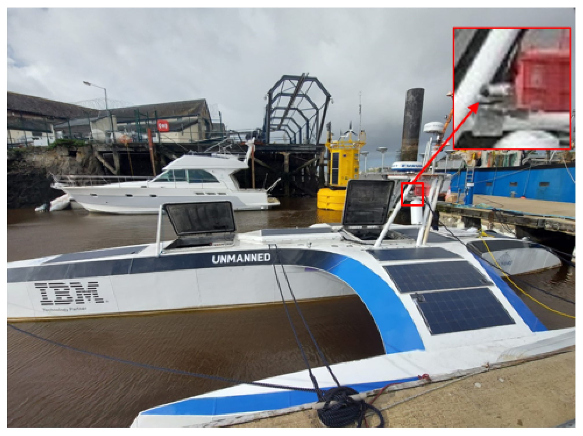
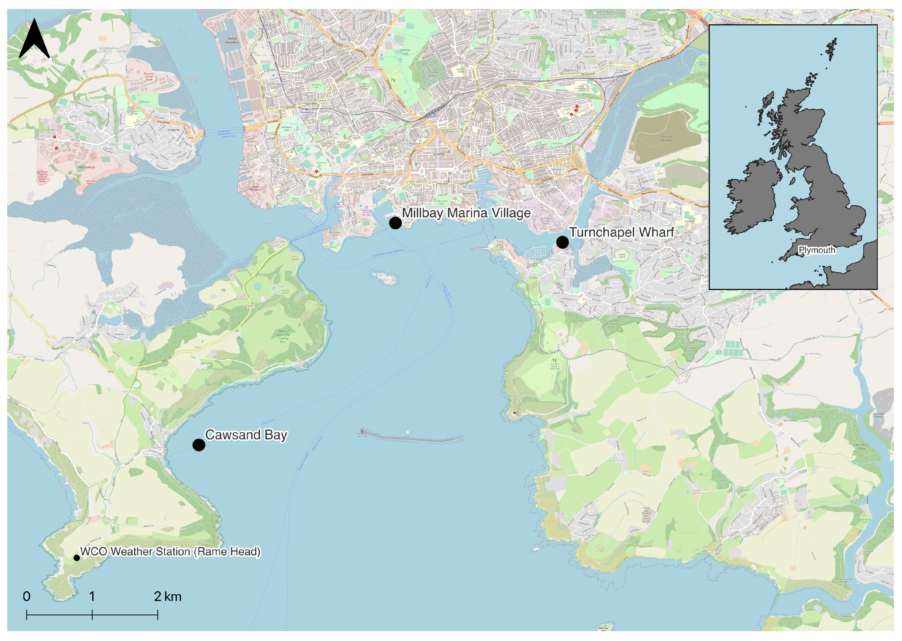
Footage of plastic in the water was collected using a video camera (Vicon Fixed Bullet camera, Model: V944B-W312MIR). This model of camera is typically used for building security, typically costs around USD 417 and is capable of collecting 2592 × 1520 pixel footage at 20 FPS. The camera was mounted on two different vessels, the MAS (Figure 2) and the Explorer (Figure 3). Footage filmed was collected on three different dates and at three different locations, as shown in Figure 4. Video from the MAS was taken whilst the vessel was moored at Turnchapel Wharf, Plymouth, UK on 20 October 2021, 2 November 2021 and 12 November 2021, filming for approximately 40–60 min at each visit. Footage of a combination of bags and bottles was filmed on both the port and starboard fixed cameras, mounted at a 90-degree angle to the sea, 2.25 m above the water as shown in Figure 2.
On the Explorer, the fixed bullet camera was attached to a davit 2.3 m above sea level, at a 90-degree angle to the sea as demonstrated in Figure 3. Footage of a combination of bags, bottles and buoys were then filmed whilst the Explorer was moored at Millbay Marina Village, Plymouth, UK (2 December 2021) and out at sea by Cawsand Bay, Cornwall, UK (25 January 2022), filming for approximately 40–60 min on both days. Plastic bags and bottles were tied together via fishing line to make recovery easier and thrown into the water in view of the camera. The Explorer then circled the plastics at approximately 3–5 knots to collect footage against varied backgrounds before the plastics were retrieved.
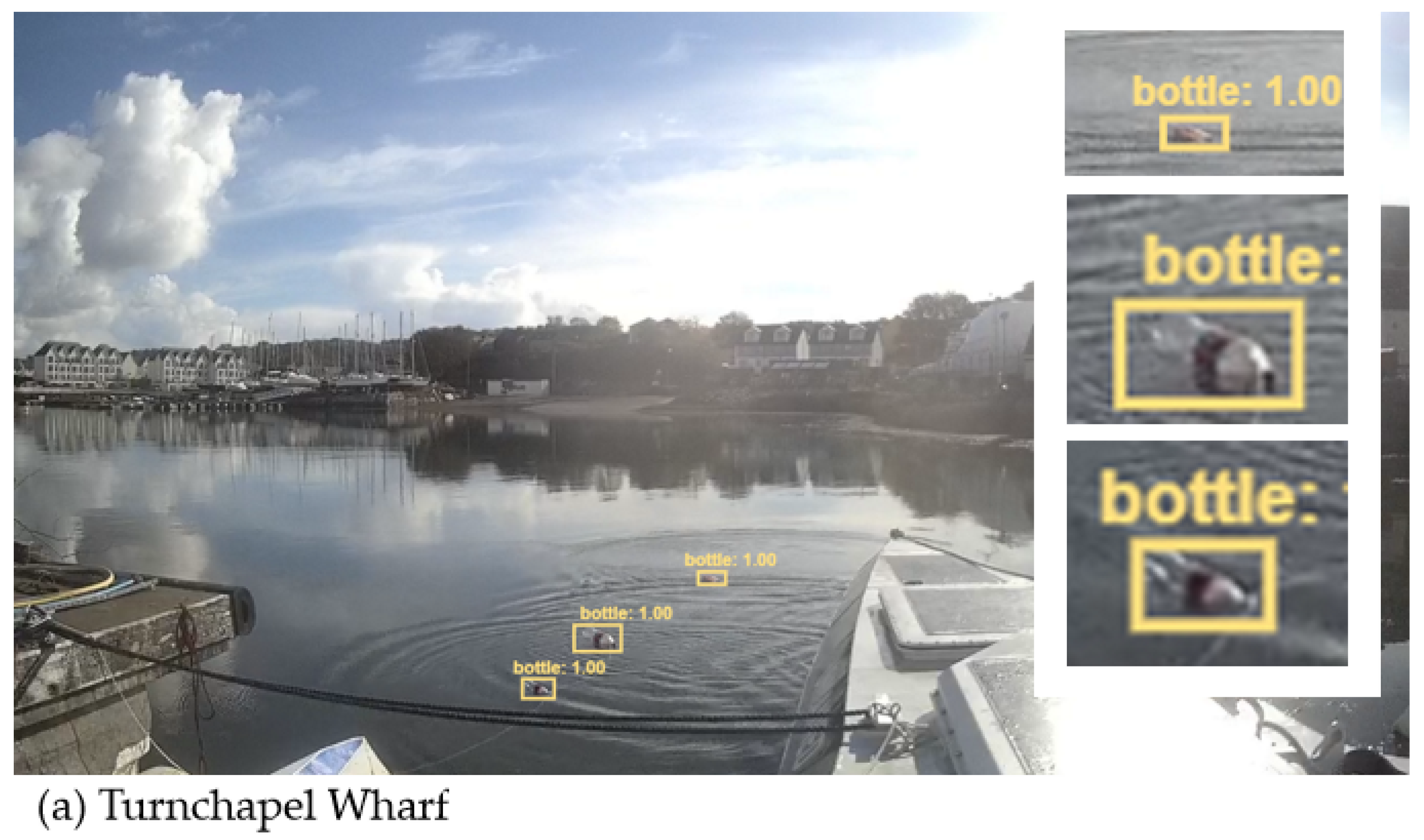
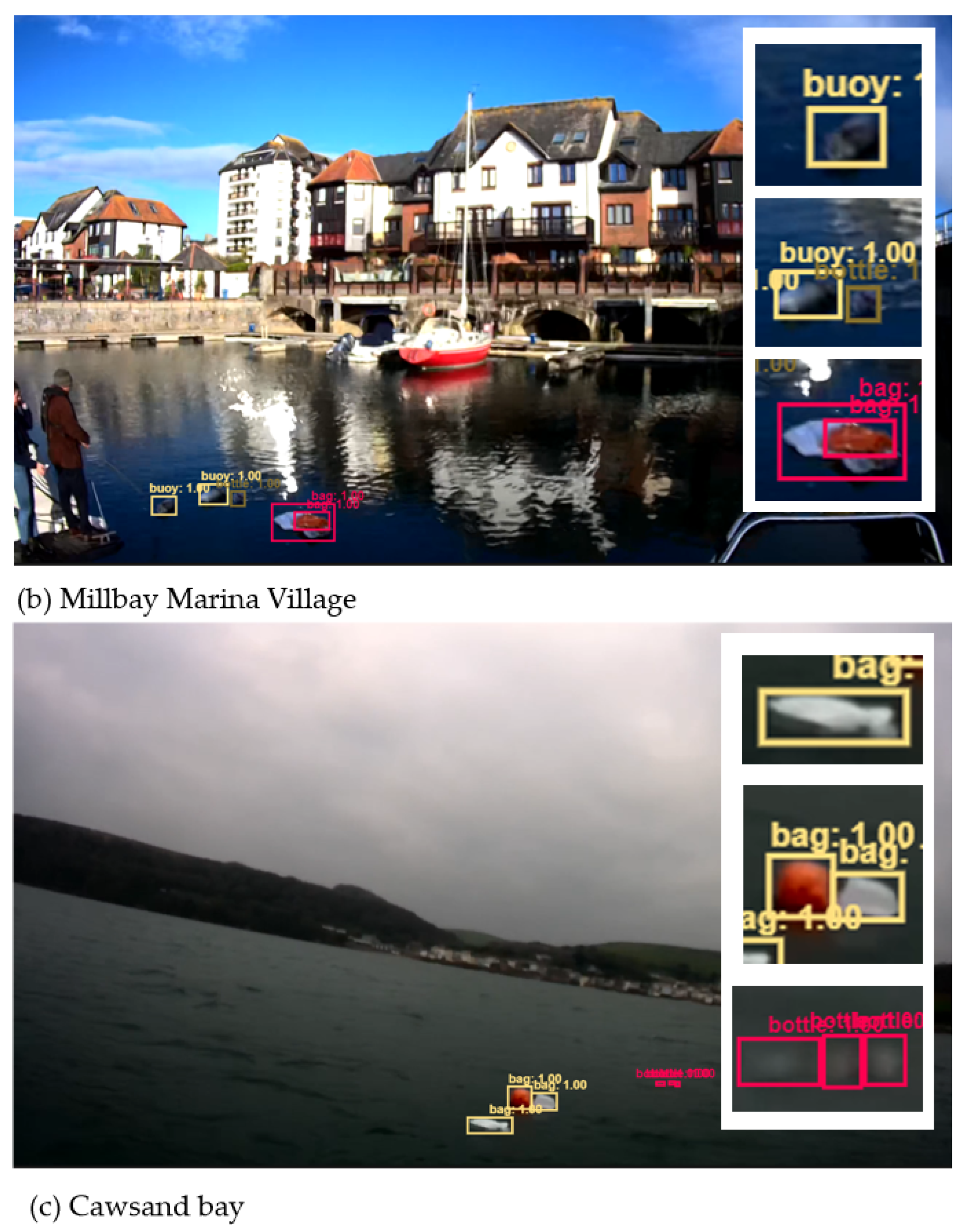
The images were collected in a variety of environmental conditions such as varied water turbidity, varied swell, cloudy and sunny days and rainy days. Specific weather conditions can be found in Table 1. When filming at the marinas on 20 October 2021, 2 November 2021, 12 November 2021 and 2 December 2021, the swell was flat. Whilst out at sea in Cawsands Bay on 25 January 2022, the swell was moderate. Data were also collected with no plastic in the water at each site. Footage from each site can be seen in in Figure 5.

2.2. Data Processing

Footage collected on the MAS and the Explorer was labeled using using the Video and Image Analytics for Multiple Environments (VIAME) software. VIAME is an open-source computer vision software platform, which is designed to aid with machine learning model training, including utilities for image and video annotation and capacity for object detection and object tracking [34]. For this study, we used the VIAME web platform to label our data set using box-level annotations. Each bounding box was drawn so that the centre of the box remained over the centre of the tracked object, as suggested in the VIAME user guide [34]. Once the videos were uploaded to VIAME, the location and category of plastics were labelled for each video at a interval of 10 frames per second. For labelling, the plastics were split into three categories: bag, bottle and buoy. The labelled data set was then exported from VIAME and separated into individual frames, with an associated label file for each frame, formatted for the YOLOv5. In total, 10,431 frames were labeled.
To increase the amount of training data, augmentation was applied using the imgaug library [35]. Augmentations applied to images included random crop, scaling, translation, shearing, horizontal flip and rotation. Additionally, a proportion of the images had linear contrast, uniform blur and brightness randomly applied. After augmentation, some images contained bounding boxes partially outside the image. To rectify this, we clipped the bounding boxes to be completely inside the image. In some images, this meant only an exceedingly small section of the plastic item remained in the image. However, we felt that this would increase the likelihood of the model detecting partially visible plastics rather than only focusing on objects that were completely within the frame.
For training, tuning and evaluating the model, we partitioned the images into training, validation and test sets. For the test set, this split was performed at the video level so no frames from the test set were used to train the model. The videos for the test data set were manually selected to represent a wide variety of conditions to evaluate if the algorithm could accurately perform in varied weather conditions with multiple plastics at different distances to the camera and with negative objects. Our test data set contained 9824 images, 30% of the overall data set. The remaining footage was then randomly split into training and validation data sets, with 19,708 (80%) of the remaining images allocated to the training data set and 4928 (20%) to the validation data set, as shown in Figure 6. Due to the lack of variation in conditions at the marinas, the frames in each video were very similar. Therefore, every 10th frame was selected from these videos for training and validation data sets. On the other hand, all the frames taken on the Explorer at sea by Cawsand Bay varied significantly due to movement on the boat. Therefore, all frames were included in the training and validation data sets along with all the augmented images from each location. After removing some of the marina footage from the data set, we had a total of 33,461 labeled frames.

2.3. Neural Network Training

To both detect and classify objects, we selected the You Only Look Once (YOLO) object detection architecture [36]. Unlike previous object detection models such as Faster R-CNN which require multiple passes over an image to generate predictions [37], YOLO is an end-to-end architecture performing object recognition and classification in a single image pass while remaining highly accurate [36]. YOLO can therefore achieve much faster training and inference speeds than previous models, with the ability to process image streams in real time (45 fps) making it ideal for high throughput object detection tasks [36,38]. YOLOv5 is an open-source framework which uses the PyTorch deep learning library to implement the most recent iteration of YOLO [39]. YOLOv5 includes several variations of the YOLO architecture ranging from small to extra large (YOLOv5s, YOLOv5m, YOLOv5l, and YOLOv5x); larger models are more complex and therefore more able to achieve higher accuracies, though at the cost of higher computational requirements [39].
To select the optimum model for our data set, several models were trained using different hyperparameters. First, we trained a model using YOLOv5s, and kept all hyperparameters in the default setting. This model was trained using 100 epochs and a batch size of 128. Loss metrics output from YOLOv5 indicated that the model converged well within 100 epochs; so further models were only trained for 50 epochs to reduce training time.
The next model was trained using the same YOLOv5s model and the same batch size and number of epoch. With the aim of trying to achieve a higher model accuracy, image size was increased from the default 640 pixels to 1280 pixels, in hopes that this would result in better detections. Next, we trained a model using the larger YOLOv5m, using 50 epochs and a batch size of 128, with an image resolution of 640. The final model trained used the YOLOv5s model and had full image resolution of 2592 pixels, trained using 50 epochs and a batch size of 32.
After analysing the performance of these models against the validation data set, the YOLOv5s model with an image size of 1280 pixels was selected as the final model due to its high accuracy with low computational input. We then ran inference over the entire test set using the chosen model.

2.4. Percentage Pixel Coverage

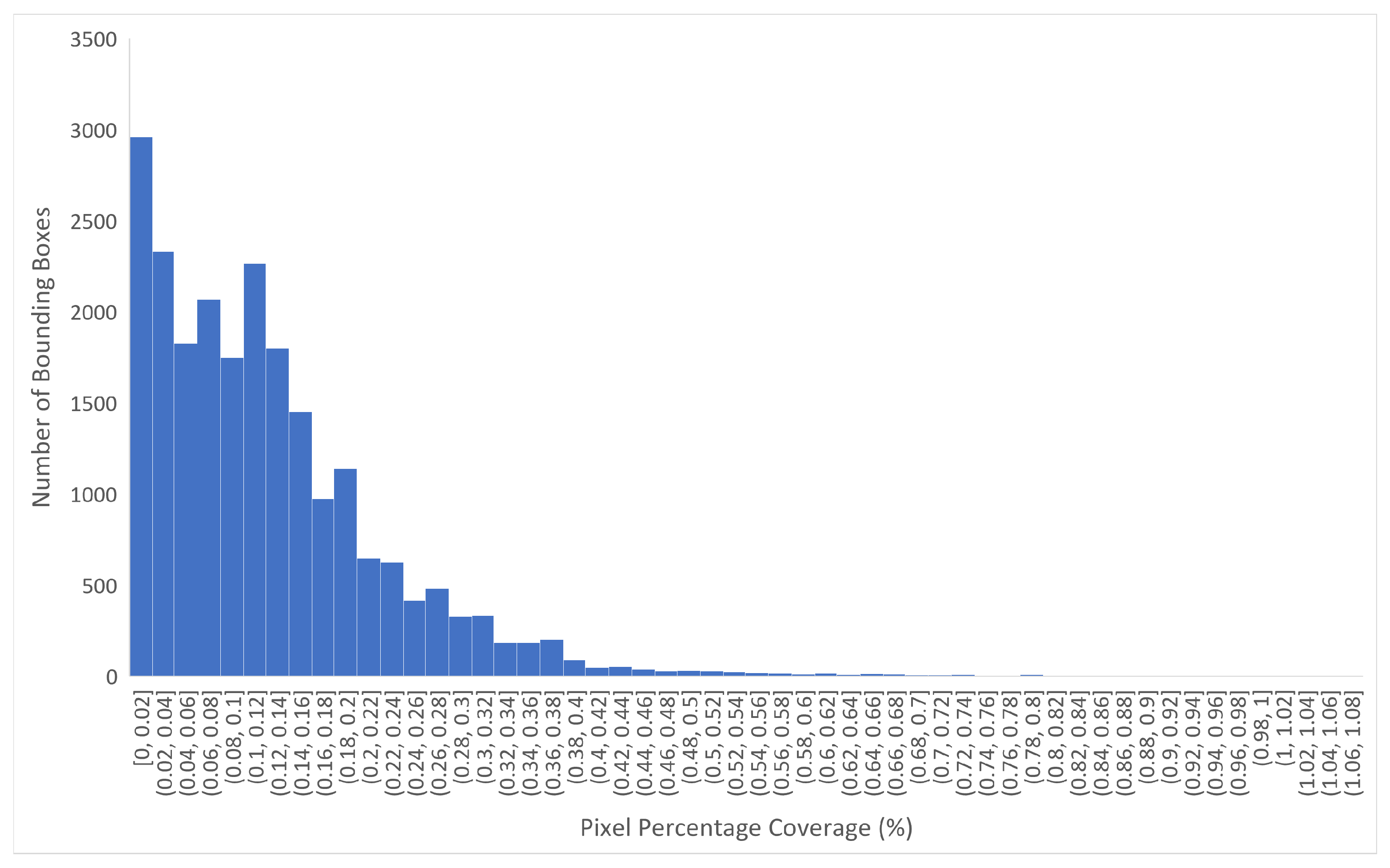
Using video footage from vessels, small plastic items (such as bottles and bags) often only occupy a small proportion of the frame. Cropping the frames (e.g., to remove non-ocean pixels) could help mitigate this; however, this would remove potentially useful contextual information, and applying such approaches is rarely straightforward as boundaries within images are often unclear. Including pre-processing steps would also reduce the transferability of the model, as the method would need to be fine-tuned for new locations and would increase detection latency. We therefore wanted to explore the effect of the plastic objects’ pixel percentage cover on the performance of the model. The percentage pixel coverage of the plastic items was calculated as the number of pixels within the bounding box of each item relative to the total number of pixels in each frame (Figure 7). By exporting the unique values of percentages into a data frame, we were able to find the 25th percentile (the threshold below which 25% of bounding boxes fell by size). For our test data set, the 25th percentile was 0.04966. This value was then used to subset the bounding boxes into a lowest 25% data set and a highest 75% data set. Because many frames contain multiple objects, frames were categorised by the size of the smallest object in the frame. Both data sets also included the test negative footage. Inference was then run over each data set. Overall, there were 4344 images in the lowest 25% data set and 6773 in the highest 75%. The accuracy of these two test data sets was then compared.

3. Results

3.1. Neural Network Performance on the Validation Data Set

As presented in Table 2, there is only a small amount of variation in the accuracy between each of the trained models. By increasing the image size from the default 640 pixels to 1280 pixels in Model 2, accuracy was slightly improved, shown by the slight rise in mAP and F1 score in comparison to Model 1. When using YOLOv5m in Model 3, accuracy remained similar to Model 2 despite the use of a larger and more complex model. Using the full image resolution in Model 4 with the YOLOv5s architecture, accuracy slightly improved compared to Model 2. Despite this slight increase in accuracy, Model 2 was chosen as the final model due to its lower computational requirements, making it more suitable for deployment.
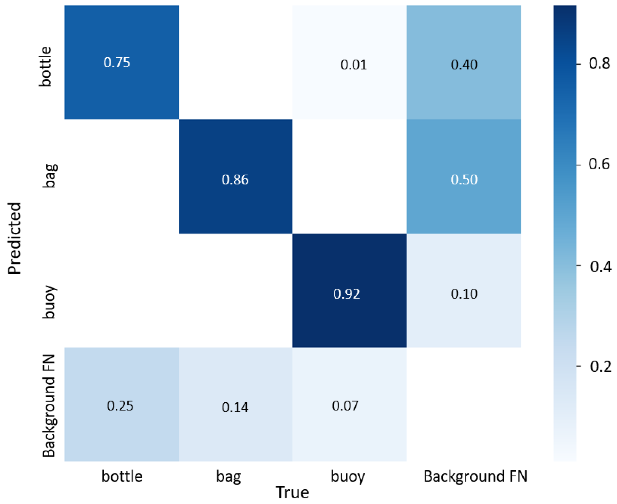
After running inference over the validation data set with the final model, the accuracy was 85.1% when differentiating between classes. When considering only the presence or absence of plastics in an image (all plastic categories combined), this accuracy increased to 95.15%. The accuracy among each class was varied, as shown in Figure 8. In the overall validation data set of 4928 images, there were 1024 false negatives. Out of these false negatives, 40% were bottles, 50% were bags and 10% were buoys. Bottles were detected as background by the model 25% of the time. This is likely due to their small size and transparency, making them difficult to distinguish from the background. Bags produced the highest proportion of false negatives; this could be due to their varied shape and tendency to sink below the surface, making them difficult to detect. It is likely that the buoys only contribute to a small proportion of false negatives due to their larger shape and high buoyancy, increasing the buoys visibility.

3.2. Neural Networks Performance on the Test Data Set

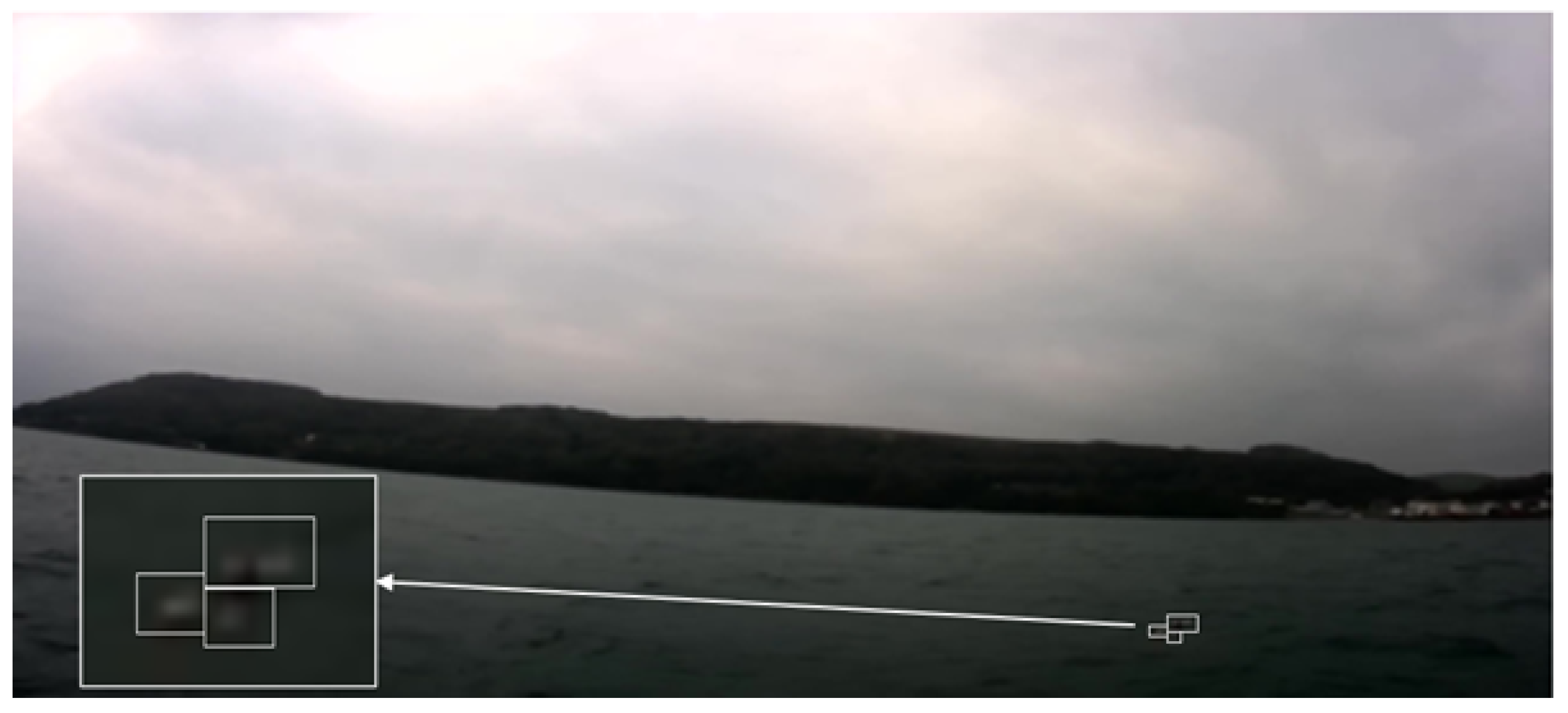
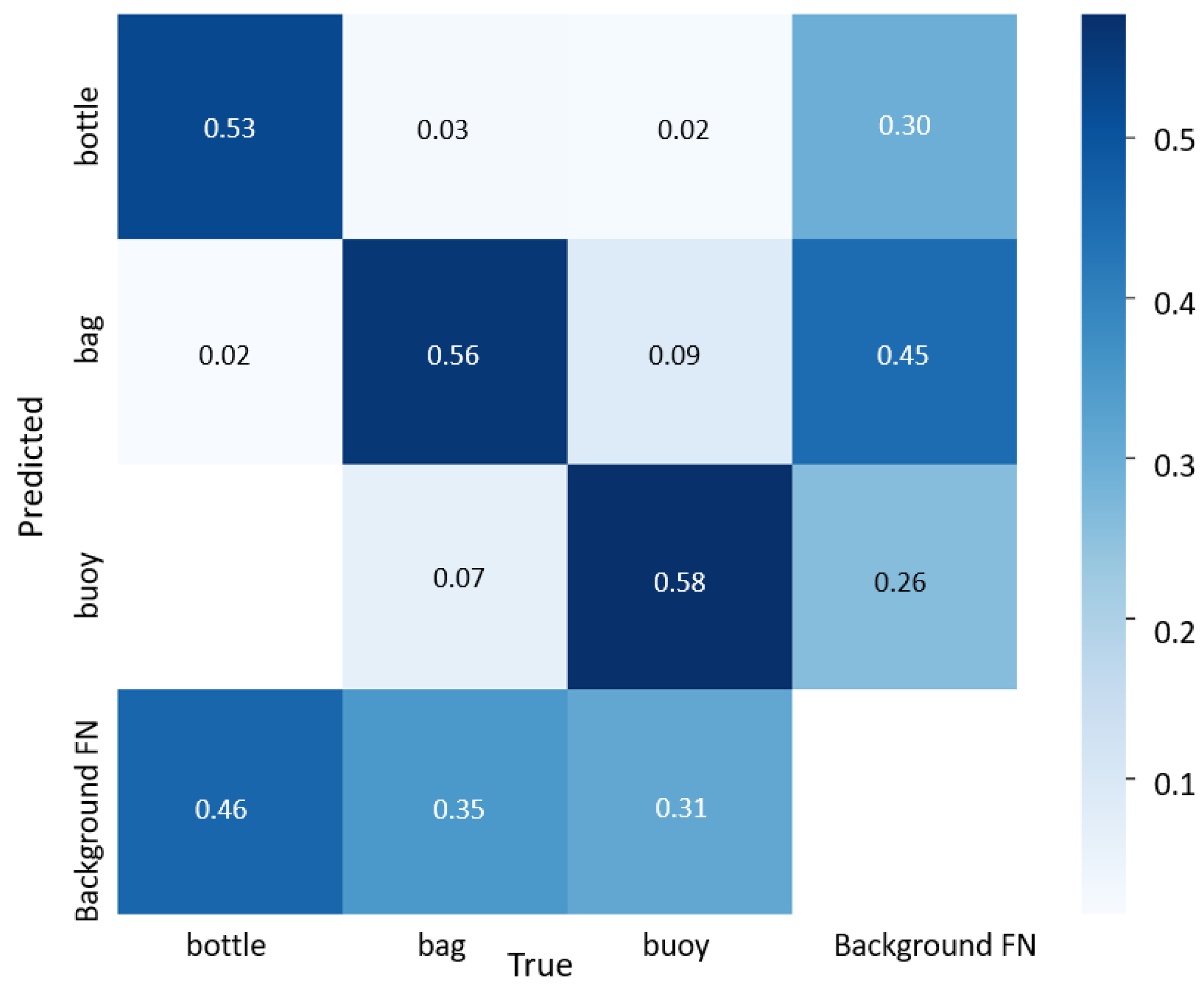
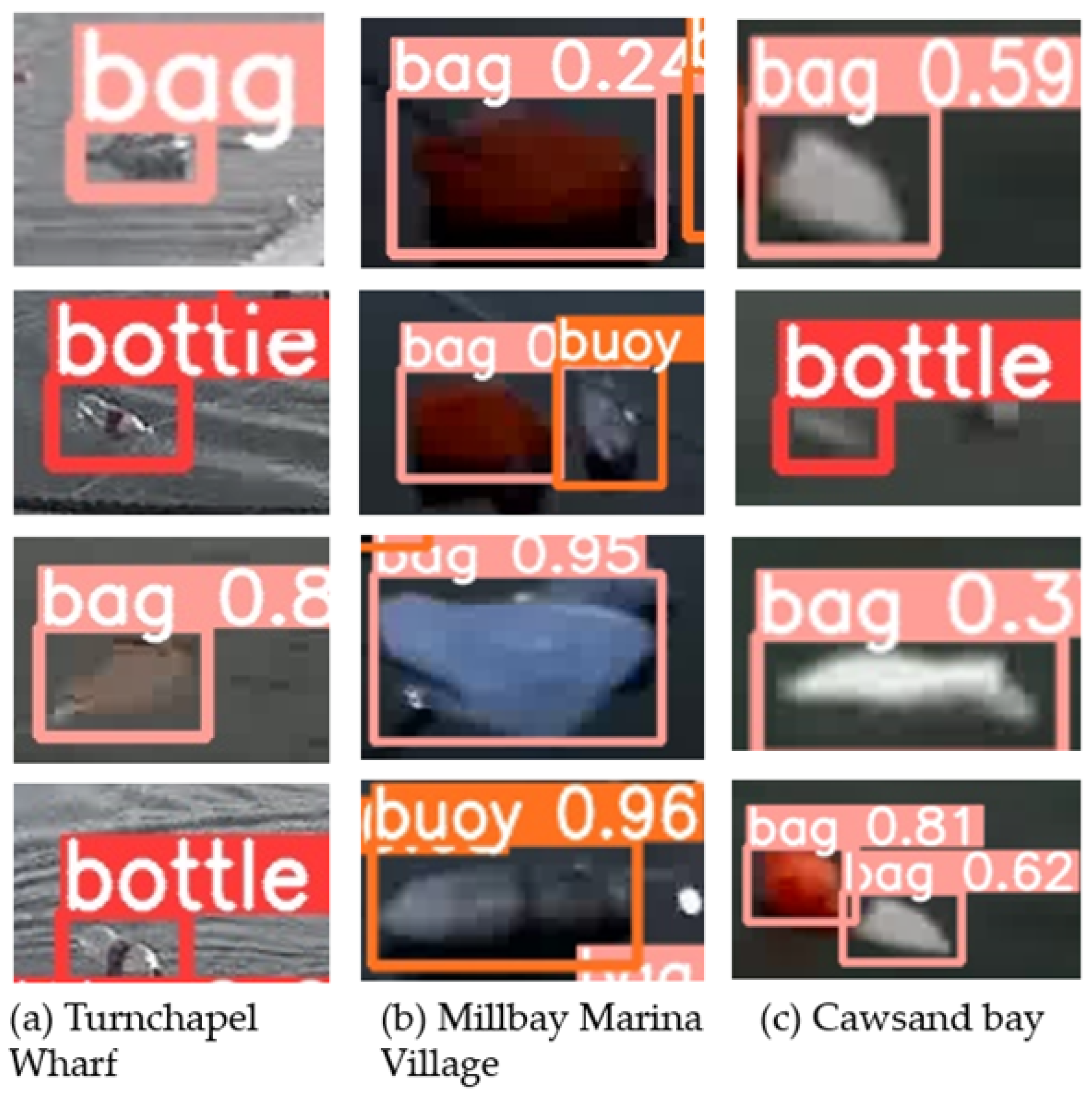
The model was 95.23% accurate at detecting the presence or absence of plastics in the test data set and validation data set. However, when differentiating between object types, the model accuracy significantly decreased to 65.3%. The model often either detected the plastic as the incorrect object type or was unable to detect the item, as shown in Table 3. When differentiating between object types, the model accuracy was significantly lower than the model accuracy from the validation data set. This is likely due to the validation data set containing frames from the same videos that were used in the training data set; however, the test data are a separate entity. The test data set represents real-world footage, which contains a large amount of variation in the environment and in the items, making the objects more difficult to detect. The class of plastic incorrectly identified as background the most was bottles, likely due to a combination of them being transparent and having a small size, making them very difficult to detect as demonstrated in Figure 9. The model successfully ignored negative objects such as vegetation debris and sun glare, as demonstrated by Figure 10. Out of the overall 9824 images in the test data set, 2280 were detected as false negatives. Of these false negatives, 30% were bottles, 44% were bags, and 26% were buoys (Figure 11). Examples of plastics successfully identified by the model are shown in Figure 12.

Percentage Pixels of Object

The results from running inference over the test data set, 25% data set and 75% data set are displayed in Table 4. By excluding 25% of the bounding boxes with the lowest pixel percentage coverage, the mAP, F1-score and precision were slightly increased. This suggests the low pixel percentage of some of the bounding boxes could be an explanation for some of the false negatives in the test data set.

4. Discussion

In this study, we successfully trained an object-detection algorithm to detect and categorise marine floating macroplastics from video footage taken with vessel-mounted cameras. Due to the low cost and accessibility of vessel-mounted cameras, this method could be used worldwide to collect in situ data on marine plastic quantification. This method also has the potential to involve citizen science and utilise autonomous ships to quantify global floating marine macroplastics.
In this study, we tested four different YOLOv5 model variations during the development stage. This included a model using the YOLOv5m architecture and three YOLOv5s models containing either the default settings, larger image size of 1280 pixels or full image resolution of 2592 pixels. The highest performing model was the YOLOv5s model with full resolution, which had an accuracy of 86.3%. The YOLOv5s model using 1280 pixels had a similar accuracy of 85.1% and was chosen as the final model, due to its significantly lower computational requirements compared to using the full resolution images. The final model was trained using 19,708 images, and validated using 4928 images.
After running inference over the validation data set, our model was able to detect the presence or absence of plastics with an accuracy of 95.15%. When differentiating between plastic categories, our model had a high accuracy of 85.1% mAP. This accuracy is similar to the YOLOv5s model created by Tata et al. (2021) [26] from their data set named DeepTrash, which had a mAP of 85% from their validation data set [26]. Contrary to our study, the validation data set created by Tata et al. (2021) [26] was mutually exclusive from the training data set, unlike our validation data set which had frames from the same video distributed in the training data set. This makes the validation data set in DeepTrash similar to our test data set, where our accuracy was much lower. This could be due to Tata et al. (2021) [26] not separating the plastics by different categories and instead having one class called ‘trash plastics’, arguable making it easier to achieve a high accuracy.
When inference was run over the test data set, which contained images unseen by the model, our model achieved a very high accuracy of 95.23% when detecting the presence or absence of plastics. Yet, when differentiating between plastic classes, the model accuracy significantly decreased to 65.3%. In addition, for images with accumulations of multiple plastics, the model often failed to identify some objects and misidentified others. Because YOLO operates in a single pass over the image, it imposes limitations on the number of objects that can be detected within a given area, reducing the capacity of the model to detect multiple small objects in close proximity [36]. While this increased the error rate, the model very rarely failed to detect any plastics where some were present. It could therefore be used as an effective pre-screening tool for identification of frames of interest in large data sets.
Whilst similar studies mentioned previously do not differentiate between plastic classes, Kylili et al. (2019) [27] provide an example of another model which does. In this study, the plastics were split into three categories, namely, plastic bottles, plastic buckets and plastic straws [27]. Their model had an accuracy of 86% over their test data set, which contained a small sample of 165 images. Despite their high model accuracy, this model has some limitations. For instance, this study was an excise of machine learning and not an actual survey. The study contained no negative samples, meaning the model was only tested on its accuracy in differentiating between classes and not on whether it can differentiate between plastics and other objects. This study is also an image classification rather than an object detection approach, which involves labelling the whole image as containing a plastic object, meaning the location of the object is not provided. This increases the requirement for manual labour because each image first needs to be cropped to the approximate location of the plastics. Although the Kylili et al. (2019) [27] study provides another example of using deep learning to classify categories of plastics, we find an object detection approach more appropriate for creating an in situ methodology to monitoring global marine macroplastics. This is due to object detection algorithms having decreased manual labour requirements, the ability to quantify the number of items and estimate their size.
By calculating the pixel percentage coverage of the bounding boxes in our test data set, we showed that the plastics the model was trying to detect made up a very small percentage of the image. This is demonstrated in Figure 7, with a majority of the bounding boxes ranging between 0–0.46% of the image. With this in consideration, the high accuracy of 95.1% is impressive. By analysing the impact of pixel percentage cover on model accuracy, we have found one potential explanation for false negative detections. In future studies, the pixel percentage cover of the objects could be increased by inputting cropped sections of the images into the model, which may decrease false negatives and computational time. However, it will decrease transferability of the model. Overfitting is another possible explanation for the number of false negative detections in this study. Overfitting occurs when the model does not generalize well from observed training data to the unseen test data [38]. An overfitting model fails to learn general rules for inference because it learns the details and noise of the training set too closely. This can be caused by the model being overly complex or because the training set does not properly approximate real-world variability [38]. In our study, some videos had frames contained in both the training data set and the validation data set, whereas the test set contained a completely independent set of videos. The lower performance on the test set therefore suggests that our training and validation sets did not capture enough environmental and contextual variability for the model to generalise well. This is not surprising given that capturing the full range of possible sea conditions is very difficult. To mitigate this problem in future studies, the training data set could be expanded through the addition of more augmented images or through the addition of more images taken in a wider variety of environmental conditions. Another possible cause for false negatives in the test data set could be that the bounding boxes in some augmented images were cropped, causing the model to struggle to detect these plastics due to their small size. Despite this, we decided to keep the bounding boxes which had been clipped, as we did not want to train the model to ignore plastics which were partially present.
Despite our model’s ability to efficiently monitor and quantify marine plastics, several improvements could be made to this study. First, our data set could be improved to represent global marine plastic debris more effectively. For instance, plastics used in this study were all sourced in England and were newly bought. To represent global marine debris, plastics from a wider range of countries could have been included, along with older plastics which have been degraded at sea. Similarly, footage collected for training and testing our model were all collected from a small regional area. For our model to be more adaptive, footage needs to be collected with a wider variety of locations, weather, wave, water turbidity and water colour illumination conditions. Additionally, to improve the representation of our model for global macroplastics, a larger range of marine plastic categories could be included in training our model, which would allow for a wider range of macroplastics to be detected during deployment. Finally, this study has the constraint that it does not define plastic categories per their composition and therefore does not comply with the proposed framework for classifying plastic debris by Hartman et al. (2019) [4]. In future studies, this constraint could be overcome through obtaining the chemical composition of macroplastics used for training.
Our methods could also be developed further through utilising multispectral cameras to detect marine floating plastics. For example, Goncalves et al. (2022) [40] investigated the use of an unmanned aerial system (UAS) to detect, map and categorise macro-litter on beaches, with 50% of the spectral references being plastics. In this study, Gonçalves et al. (2022) [40] showed that multispectral images collected by drones can support automated categorization of stranded litter material. Using similar techniques, vessel-mounted multispectral instruments could be explored as an alternative or complementary method of monitoring in situ floating marine debris as long as plastics are above the water surface and the appropriate wavelengths are targeted [41]. This approach could also be explored for detecting marine microplastics if a video could be recorded with a microscope. Currently there is no standard procedure for sampling, counting and confirming the presence of microplastics in the current literature, resulting in difficulties when comparing microplastic abundance between studies [42].

5. Conclusions and Recommendations

Using video cameras mounted on small vessels, we were able to detect the presence of plastics using an object-detection algorithm with an accuracy of 95.2%. Additionally, our model was able to differentiate between three predefined categories with an accuracy of 65.3%. By calculating the pixel percentage coverage of the bounding boxes in our data set, we showed that the plastics the model was trying to detect made up a very small percentage of the image, ranging between 0.0006–0.46%. We found that the images containing these smaller plastics negatively affected model accuracy. Pre-processing methods to increase the percentage cover of plastics in the image, for example through scaling or cropping, could potentially overcome this issue. However, the benefit of potentially increasing model accuracy with pre-processing methods needs to be evaluated with the cost of reduced transferability of the model, as the method would need to be fine-tuned for new locations and would increase detection latency. Despite the decreased accuracy of our model when differentiating between classes, the model very rarely failed to detect any plastics where some were present even though a majority of the plastics covered a very small proportion of the image. It could therefore be used as an effective pre-screening tool for identification of frames of interest in large data sets. Overall, this study demonstrated a novel approach to collecting harmonised in situ data through using an object-detection algorithm and boat-mounted camera. Our approach was novel due to our data collection method of using a boat-mounted camera and machine learning, training our algorithm to distinguish between plastic classes, using unseen real-world footage for testing and exploring pixel percentage coverage of the plastic items as an explanation for false negatives. This study also provided further evidence that YOLOv5s is a fast, efficient and precise model for detecting marine macroplastics. The data set generated will provide a foundation for future studies utilising vessel-mounted cameras for plastics detection.

Author Contributions

Conceptualization, V.M.-V.; methodology, V.M.-V., K.A.-C., S.A. and D.C.; software, K.A.-C., D.C. and S.A.; validation, K.A.-C., D.C. and S.A.; formal analysis, K.A.-C., D.C. and S.A.; investigation, V.M.-V., K.A.-C., D.C. and S.A.; resources, D.C.; data curation, K.A.-C., D.C. and S.A.; writing—original draft preparation, S.A.; writing—review and editing, S.A., K.A.-C., V.M.-V. and D.C.; visualization, S.A. and K.A.-C.; supervision, V.M.-V.; project administration, V.M.-V.; funding acquisition, V.M.-V. All authors have read and agreed to the published version of the manuscript.

Funding

Funding for this study was provided through the Plymouth Marine Laboratory internal research program. Computational resources on the MASsive GPU for Earth Observation (MAGEO) cluster were provided through the NERC Earth Observation Data Acquisition and Analysis Service (NEODAAS). V.M.-V. has been supported by European Space Agency (ESA) grant number 40000123928/18/I-NB, SIMPLER: SensIng Marine Plastic Litter using Earth observation in River outflows and ESA Discovery Campaign “Remote Sensing of Plastic Marine Litter” grant number 4000132212/20/NL/GLC.

Data Availability Statement

Not applicable.

Acknowledgments

We would like to thank the team at Marine AI, specifically Oliver Thompson, Benjamin Wickenden and Matthew Shaw for facilitating and assisting with the filming on the Mayflower Autonomous Ship. We would like to thank Oban Jones at PML for facilitating the tests at sea using the PML Explorer. We thank four anonymous reviewers for their time and comments that helped to improve the quality of this manuscript. We would also like to thank The Western Channel Observatory for supplying historical weather data used in Table 1. The Western Channel Observatory is funded by the UK Natural Environment Research Council through its National Capability Long-term Single Centre Science Programme, Climate Linked Atlantic Sector Science, grant number NE/R015953/.

Conflicts of Interest

The authors declare no conflict of interest. The funders had no role in the design of the study; in the collection, analyses, or interpretation of data; in the writing of the manuscript, or in the decision to publish the results.

References

  1. Gregory, M.R.; Ryan, P.G. Pelagic Plastics and Other Seaborne Persistent Synthetic Debris: A Review of Southern Hemisphere Perspectives. In Marine Debris: Sources, Impacts, and Solutions; Coe, J.M., Rogers, D.B., Eds.; Springer Series on Environmental Management; Springer: New York, NY, USA, 1997; pp. 49–66. [Google Scholar] [CrossRef]
  2. Jambeck, J.R.; Geyer, R.; Wilcox, C.; Siegler, T.R.; Perryman, M.; Andrady, A.; Narayan, R.; Law, K.L. Plastic waste inputs from land into the ocean. Science 2015, 347, 768–771. [Google Scholar] [CrossRef]
  3. Sivan, A. New perspectives in plastic biodegradation. Curr. Opin. Biotechnol. 2011, 22, 422–426. [Google Scholar] [CrossRef]
  4. Hartmann, N.B.; Hüffer, T.; Thompson, R.C.; Hassellöv, M.; Verschoor, A.; Daugaard, A.E.; Rist, S.; Karlsson, T.; Brennholt, N.; Cole, M.; et al. Are We Speaking the Same Language? Recommendations for a Definition and Categorization Framework for Plastic Debris. Environ. Sci. Technol. 2019, 53, 1039–1047. [Google Scholar] [CrossRef] [Green Version]
  5. Azzarello, M.Y.; Vleet, E.S.V. Marine birds and plastic pollution. Mar. Ecol. Prog. Ser. 1987, 37, 295–303. [Google Scholar] [CrossRef]
  6. McCauley, S.J.; Bjorndal, K.A. Conservation Implications of Dietary Dilution from Debris Ingestion: Sublethal Effects in Post-Hatchling Loggerhead Sea Turtles. Conserv. Biol. 1999, 13, 925–929. [Google Scholar] [CrossRef]
  7. Gregory, M.R. Environmental implications of plastic debris in marine settings—entanglement, ingestion, smothering, hangers-on, hitch-hiking and alien invasions. Philos. Trans. R. Soc. B Biol. Sci. 2009, 364, 2013–2025. [Google Scholar] [CrossRef]
  8. Fossi, M.C.; Marsili, L.; Baini, M.; Giannetti, M.; Coppola, D.; Guerranti, C.; Caliani, I.; Minutoli, R.; Lauriano, G.; Finoia, M.G.; et al. Fin whales and microplastics: The Mediterranean Sea and the Sea of Cortez scenarios. Environ. Pollut. 2016, 209, 68–78. [Google Scholar] [CrossRef]
  9. Provencher, J.F.; Vermaire, J.C.; Avery-Gomm, S.; Braune, B.M.; Mallory, M.L. Garbage in guano? Microplastic debris found in faecal precursors of seabirds known to ingest plastics. Sci. Total Environ. 2018, 644, 1477–1484. [Google Scholar] [CrossRef]
  10. Guerrera, M.C.; Aragona, M.; Porcino, C.; Fazio, F.; Laurà, R.; Levanti, M.; Montalbano, G.; Germanà, G.; Abbate, F.; Germanà, A. Micro and Nano Plastics Distribution in Fish as Model Organisms: Histopathology, Blood Response and Bioaccumulation in Different Organs. Appl. Sci. 2021, 11, 5768. [Google Scholar] [CrossRef]
  11. Messinetti, S.; Mercurio, S.; Parolini, M.; Sugni, M.; Pennati, R. Effects of polystyrene microplastics on early stages of two marine invertebrates with different feeding strategies. Environ. Pollut. 2018, 237, 1080–1087. [Google Scholar] [CrossRef]
  12. Eriksen, M.; Lebreton, L.C.M.; Carson, H.S.; Thiel, M.; Moore, C.J.; Borerro, J.C.; Galgani, F.; Ryan, P.G.; Reisser, J. Plastic Pollution in the World’s Oceans: More than 5 Trillion Plastic Pieces Weighing over 250,000 Tons Afloat at Sea. PLoS ONE 2014, 9, e111913. [Google Scholar] [CrossRef] [PubMed] [Green Version]
  13. Rothäusler, E.; Jormalainen, V.; Gutow, L.; Thiel, M. Low abundance of floating marine debris in the northern Baltic Sea. Mar. Pollut. Bull. 2019, 149, 110522. [Google Scholar] [CrossRef]
  14. Sá, S.; Bastos-Santos, J.; Araújo, H.; Ferreira, M.; Duro, V.; Alves, F.; Panta-Ferreira, B.; Nicolau, L.; Eira, C.; Vingada, J. Spatial distribution of floating marine debris in offshore continental Portuguese waters. Mar. Pollut. Bull. 2016, 104, 269–278. [Google Scholar] [CrossRef]
  15. Maximenko, N.; Corradi, P.; Lavender Law, K.; Van Sebille, E.; Shungudzemwoyo, P.G.; Lampitt, R.S.; Galgani, F.; Martinez_vincente, V.; Goddijn-Murphy, L.; Veiga, J.M.; et al. Towards the Integrated Marine Debris Observing System. Front. Mar. Sci. 2019, 6, 447. [Google Scholar] [CrossRef] [Green Version]
  16. Garcia-Garin, O.; Monleón-Getino, T.; López-Brosa, P.; Borrell, A.; Aguilar, A.; Borja-Robalino, R.; Cardona, L.; Vighi, M. Automatic detection and quantification of floating marine macro-litter in aerial images: Introducing a novel deep learning approach connected to a web application in R. Environ. Pollut. 2021, 273, 116490. [Google Scholar] [CrossRef] [PubMed]
  17. Unger, B.; Herr, H.; Viquerat, S.; Gilles, A.; Burkhardt-Holm, P.; Siebert, U. Opportunistically collected data from aerial surveys reveal spatio-temporal distribution patterns of marine debris in German waters. Environ. Sci. Pollut. Res. 2021, 28, 2893–2903. [Google Scholar] [CrossRef] [PubMed]
  18. Geraeds, M.; van Emmerik, T.; de Vries, R.; bin Ab Razak, M.S. Riverine Plastic Litter Monitoring Using Unmanned Aerial Vehicles (UAVs). Remote Sens. 2019, 11, 2045. [Google Scholar] [CrossRef] [Green Version]
  19. van Lieshout, C.; van Oeveren, K.; van Emmerik, T.; Postma, E. Automated River Plastic Monitoring Using Deep Learning and Cameras. Earth Space Sci. 2020, 7, e2019EA000960. [Google Scholar] [CrossRef]
  20. de Vries, R.; Egger, M.; Mani, T.; Lebreton, L. Quantifying Floating Plastic Debris at Sea Using Vessel-Based Optical Data and Artificial Intelligence. Remote Sens. 2021, 13, 3401. [Google Scholar] [CrossRef]
  21. Gonçalves, G.; Andriolo, U. Operational use of multispectral images for macro-litter mapping and categorization by Unmanned Aerial Vehicle. Mar. Pollut. Bull. 2022, 176, 113431. [Google Scholar] [CrossRef]
  22. Garaba, S.P.; Aitken, J.; Slat, B.; Dierssen, H.M.; Lebreton, L.; Zielinski, O.; Reisser, J. Sensing Ocean Plastics with an Airborne Hyperspectral Shortwave Infrared Imager. Environ. Sci. Technol. 2018, 52, 11699–11707. [Google Scholar] [CrossRef] [PubMed]
  23. Freitas, S.; Silva, H.; Silva, E. Remote Hyperspectral Imaging Acquisition and Characterization for Marine Litter Detection. Remote Sens. 2021, 13, 2536. [Google Scholar] [CrossRef]
  24. Garcia-Garin, O.; Aguilar, A.; Borrell, A.; Gozalbes, P.; Lobo, A.; Penadés-Suay, J.; Raga, J.A.; Revuelta, O.; Serrano, M.; Vighi, M. Who’s better at spotting? A comparison between aerial photography and observer-based methods to monitor floating marine litter and marine mega-fauna. Environ. Pollut. 2020, 258, 113680. [Google Scholar] [CrossRef]
  25. Garcia-Garin, O.; Borrell, A.; Aguilar, A.; Cardona, L.; Vighi, M. Floating marine macro-litter in the North Western Mediterranean Sea: Results from a combined monitoring approach. Mar. Pollut. Bull. 2020, 159, 111467. [Google Scholar] [CrossRef] [PubMed]
  26. Tata, G.; Royer, S.J.; Poirion, O.; Lowe, J. A Robotic Approach towards Quantifying Epipelagic Bound Plastic Using Deep Visual Models. arXiv 2021, arXiv:2105.01882. [Google Scholar]
  27. Kylili, K.; Kyriakides, I.; Artusi, A.; Hadjistassou, C. Identifying floating plastic marine debris using a deep learning approach. Environ. Sci. Pollut. Res. 2019, 26, 17091–17099. [Google Scholar] [CrossRef] [PubMed]
  28. Majaj, N.J.; Pelli, D.G. Deep learning—Using machine learning to study biological vision. J. Vis. 2018, 18, 2. [Google Scholar] [CrossRef] [Green Version]
  29. Wäldchen, J.; Mäder, P. Machine learning for image based species identification. Methods Ecol. Evol. 2018, 9, 2216–2225. [Google Scholar] [CrossRef]
  30. Albawi, S.; Mohammed, T.A.; Al-Zawi, S. Understanding of a convolutional neural network. In Proceedings of the 2017 International Conference on Engineering and Technology (ICET), Antalya, Turkey, 21–23 August 2017; pp. 1–6. [Google Scholar] [CrossRef]
  31. Tata, G. Using Deep Learning to Quantify, Monitor, and Remove Marine Plastic; Towards Data Science: Toronto, ON, Canada, 2021. [Google Scholar]
  32. European Commission. Joint Research Centre. Joint List of Litter Categories for Marine Macro-Litter Monitoring: Manual for the Application of the Classification System; Publications Office: Luxembourg, 2021. [Google Scholar]
  33. Current Weather Conditions at Rame Head NCI. Nci-ramehead.org.uk. 2022. Available online: http://www.nci-ramehead.org.uk/weather/archive/ (accessed on 1 June 2022).
  34. VIAME/VIAME: Video and Image Analytics for Marine Environments. GitHub - VIAME/VIAME: Video and Image Analytics for Multiple Environments [Internet]. GitHub. 2022. Available online: https://github.com/VIAME/VIAME (accessed on 1 June 2022).
  35. Imgaug—Imgaug 0.4.0. Available online: https://https://imgaug.readthedocs.io/en/latest/index.html (accessed on 1 June 2022).
  36. Redmon, J.; Divvala, S.; Girshick, R.; Farhadi, A. You Only Look Once: Unified, Real-Time Object Detection. In Proceedings of the IEEE Conference on Computer Vision and Pattern Recognition, Las Vegas, NV, USA, 27–30 June 2016. [Google Scholar] [CrossRef] [Green Version]
  37. Ren, S.; He, K.; Girshick, R.; Sun, J. Faster R-CNN Towards real-time object detection with region proposal networks. IEEE Trans. Pattern Anal. Mach. Intell. 2017, 39, 1137–1149. [Google Scholar] [CrossRef] [Green Version]
  38. Ying, X. An Overview of Overfitting and its Solutions. J. Phys. Conf. Ser. 2019, 1168, 022022. [Google Scholar] [CrossRef]
  39. GitHub—ultralytics/yolov5: YOLOv5 in PyTorch > ONNX > CoreML > TFLite. GitHub. 2022. Available online: https://github.com/ultralytics/yolov5 (accessed on 1 June 2022).
  40. Gonçalves, G.; Andriolo, U.; Gonçalves, L.; Sobral, P.; Bessa, F. Quantifying Marine Macro Litter Abundance on a Sandy Beach Using Unmanned Aerial Systems and Object-Oriented Machine Learning Methods. Remote Sens. 2020, 12, 2599. [Google Scholar] [CrossRef]
  41. Garaba, S.; Dierssen, H. An airborne remote sensing case study of synthetic hydrocarbon detection using short wave infrared absorption features identified from marine-harvested macro- and microplastics. Remote Sens. Environ. 2018, 205, 224–235. [Google Scholar] [CrossRef]
  42. Ricciardi, M.; Pironti, C.; Motta, O.; Miele, Y.; Proto, A.; Montano, L. Microplastics in the Aquatic Environment: Occurrence, Persistence, Analysis, and Human Exposure. Water 2021, 13, 973. [Google Scholar] [CrossRef]
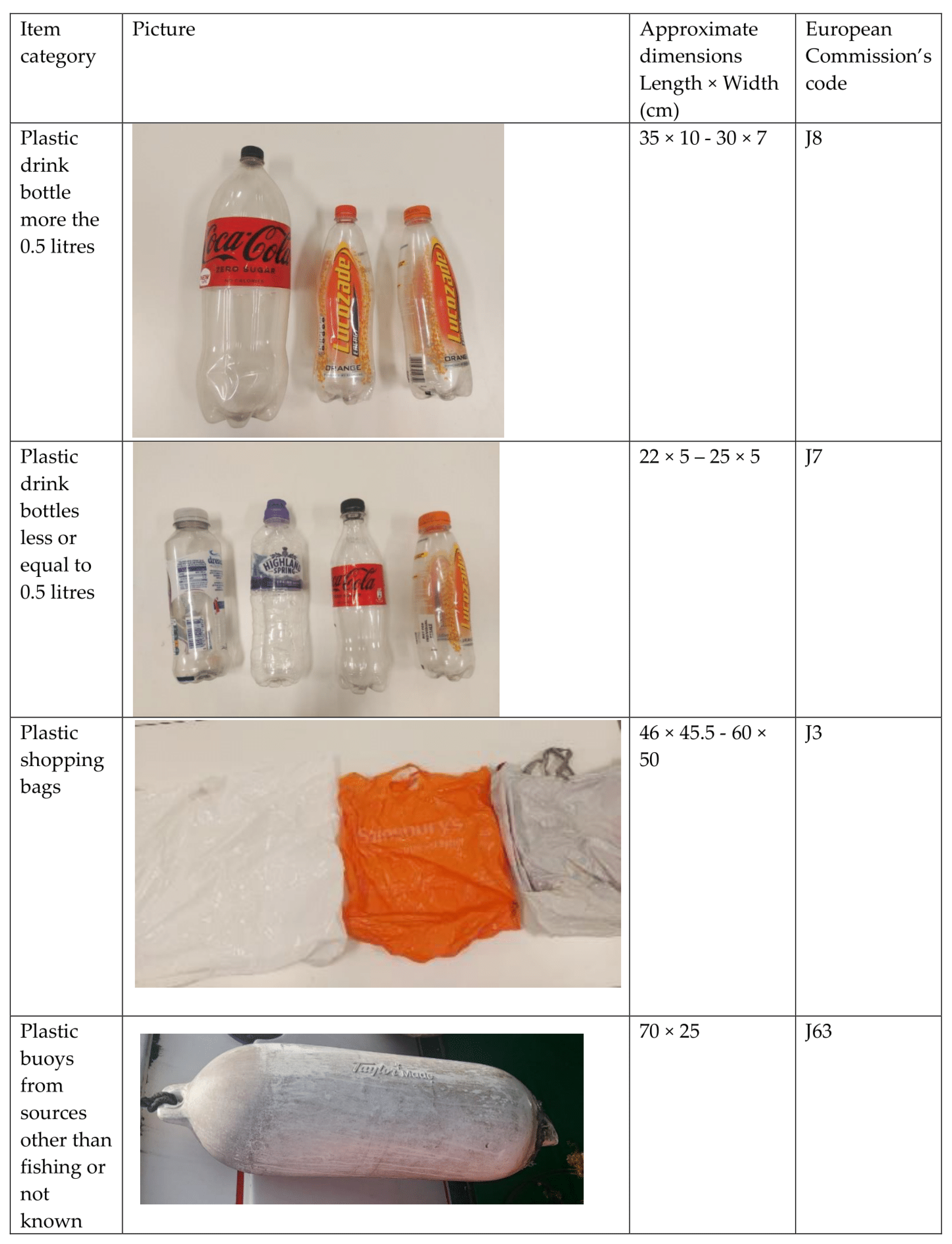
Figure 1. Table displaying objects used for filming, the approximate dimensions for each item and the Commission’s Joint List of Litter Categories for Marine Macrolitter monitoring code for each category [32].
Remotesensing 14 03425 g001
Figure 2. Camera setup on the MAS. There is a Vicon security camera on both the port and starboard sides of the boat, 2.25 m above sea level, facing at a 90-degree angle to the sea. The port-side camera is visible in this image, as highlighted in the box drawn on the image.
Remotesensing 14 03425 g002
Figure 3. Camera setup on the Explorer whilst moored at Millbay marina. A Vicon fixed bullet camera is attached to a davit on the Explorer, faced at a 90-degree angle to the sea. The footage is streamed onto the computer using an Ethernet cable.
Remotesensing 14 03425 g003
Figure 4. Map of sample sites showing the location of Turnchapel Wharf, Millbay Marina and Cawsand Bay. All sample sites are located in the southwest of England, specifically Devon and Cornwall. Background OpenStreetMap, © OpenStreetMap contributors.
Remotesensing 14 03425 g004
Figure 5. Training images containing plastic items used for training from (a) Turnchapel Wharf, (b) Millbay Marina Village and (c) Cawsand Bay. The image from Turnchapel Wharf is taken on the MAS and contains three transparent bottles. The image at Millbay Marina Village is taken on the Explorer. Two buoys and two bags can be seen in this image. The image taken from Cawsand Bay is taken on the MAS. This image contains three bags, two white and one orange. The image also contains three transparent bottles.
Remotesensing 14 03425 g005aRemotesensing 14 03425 g005b
Figure 6. Overview of methods used to create the object detection algorithm.
Remotesensing 14 03425 g006
Figure 7. Histogram showing the distribution of pixel percentage cover of the plastic items in comparison to overall image size in the test data set.
Remotesensing 14 03425 g007
Figure 8. Normalised confusion matrix showing the output from the final model run over the validation data set. Bottles were predicted correctly by the model 75% of the time, and bottles were incorrectly identified as background 25% of the time. Bags were correctly identified by the model 86% of the time and wrongly identified as background 14% of the time. Buoys were correctly identified 92% of the time and misidentified as background 7% of the time.
Remotesensing 14 03425 g008
Figure 9. Example of one of the false negative images from the validation data set. The image contains three small bottles which have drifted away from the vessel. The percentage cover of each bounding box is 0.033%, 0.015% and 0.007%.
Remotesensing 14 03425 g009
Figure 10. Test images containing negative objects such as vegetation debris and sun glare as labelled on the image. The model ignored these objects and detected the three plastic bottles as shown in the image.
Remotesensing 14 03425 g010
Figure 11. Normalised confusion matrix showing the output from the final model run over the test data set. Bottles were predicted correctly by the model 53% of the time, and bottles were incorrectly identified as background 46% of the time. Bags were correctly identified by the model 56% of the time and wrongly identified as background 35% of the time. Buoys were correctly identified 58% of the time and misidentified as background 31% of the time.
Remotesensing 14 03425 g011
Figure 12. Zoomed in test images from each site showing the plastics detected by the model for each of the three sites (a) Turnchapel Wharf, (b) Millbay Marina Village, (c) Cawsand bay.
Remotesensing 14 03425 g012
Table 1. Weather conditions on days of filming including the minimum and maximum temperature, average wind speed and minimum and maximum rainfall at time of filming. Data used in this table is provided by the Western Channel Observatory [33], collected from the weather station located on Rame Head, Cornwall. The weather station location is shown in Figure 4.
Date (Day/Month/Year)Min-Max Temperature
(Degrees Celsius)
Average Wind Speed (mph)Min-Max Rainfall (mm)
20 October 202114.7–14.828.90.00
2 November 202111.8–11.92.90.00
12 November 202112.1–12.321.90.00
2 December 20215.8–6.014.20.00–0.2
25 January 20226.4–6.313.00.00
Table 2. Performance metrics of each model tested. Results were created after running inference over the validation data set. Model 1 was run using YOLOv5s, default settings, 100 epochs and 128 batch size. Model 2 was run using YOLOv5s, 1280 pixels, 100 epochs and 128 batch size. Model 3 was run using YOLOv5m, 640 resolution, 50 epochs and 128 batch size. Model 4 was run using YOLOv5s, 2592 resolution, 50 epochs and 32 batch size. Table 1 presents the mean average precision, F1-score, precision and recall of each model.
ModelmAPF1-scorePrecisionRecall
Model 1 (v5s, 640)0.8330.840.9810.86
Model 2 (v5s, 1280)0.8510.850.9770.88
Model 3 (v5m, 640)0.8470.850.9760.87
Model 4 (v5s, 2592)0.8630.860.9520.90
Table 3. Quantity of plastic correctly identified, misidentified as the incorrect class or not identified by the model. The table shows these quantities for the bottles, bags, buoys and total plastics from the test data set. The number of plastics refers to how many times the model has detected a plastic item. Many of these detections will be from the same plastic item counted multiple times.
Model DetectionBottleBagBuoyTotal
Correct30636630267312,366
Incorrect class3995057751679
False negative67410165904953
Table 4. Performance metrics of the final model after inference over the entire test data set, the data containing the bounding boxes with the lowest 25% percentage coverage and the data set containing the bounding boxes with the highest 75% percentage coverage within the test data set. Table 2 presents the mean average precision, f1-score, precision and recall of each model.
Data SetmAPF1-ScorePrecisionRecall
Overall Test0.6530.640.9790.75
75% Test0.660.650.9790.73
25% Test0.5150.520.9780.66
Publisher’s Note: MDPI stays neutral with regard to jurisdictional claims in published maps and institutional affiliations.