Abstract
There is a growing demand to train Earth Observation (EO) data users in how to access and use existing and upcoming data. A promising tool for data-related training is computational notebooks, which are interactive web applications that combine text, code and computational output. Here, we present the Learning Tool for Python (LTPy), which is a training course (based on Jupyter notebooks) on atmospheric composition data. LTPy consists of more than 70 notebooks and has taught over 1000 EO data users so far, whose feedback is overall positive. We adapted five guiding principles from different fields (mainly scientific computing and Jupyter notebook research) to make the Jupyter notebooks more educational and reusable. The Jupyter notebooks developed (i) follow the literate programming paradigm by a text/code ratio of 3, (ii) use instructional design elements to improve navigation and user experience, (iii) modularize functions to follow best practices for scientific computing, (iv) leverage the wider Jupyter ecosystem to make content accessible and (v) aim for being reproducible. We see two areas for future developments: first, to collect feedback and evaluate whether the instructional design elements proposed meet their objective; and second, to develop tools that automatize the implementation of best practices.
1. Introduction
There is a growing gap between the amount of open Earth Observation (EO) data produced every day and the ability of users to find, access and process the data. Growing data volumes, data discovery and a limited processing capacity are major challenges faced by users of EO data, and these problems hinder data uptake and use []. Hence, there is a growing need to inform EO data users about existing and upcoming data products, as well as to teach them how to access and work with them. This aspect will gain importance in the future, as many new developments and missions are in the pipeline. During the second phase of the Copernicus program, the launches of six high-priority candidate missions are planned by 2027 [,]. The European Organisation for the Exploitation of Meteorological Satellites (EUMETSAT) is preparing the launch of the next generation of its geostationary (Meteosat Third Generation) and polar-orbiting (Metop-Second Generation (SG)) satellites [], and NASA’s Landsat program continues with the launch of Landsat-9 in September 2021 [], followed by Landsat NeXt in 2029 [].
EO training is developed and offered by different entities, including academia, commercial entities and key organizations in the field such as the National Aeronautical and Space Agency (NASA) in the US or the European Space Agency (ESA) and EUMETSAT in Europe. EO training offered through academia (category 1) provides a general introduction and formal training in basic and advanced concepts of remote sensing, geographic information sciences (GIS) and machine learning (ML) [,]. This category additionally teaches foundational technical skills such as data management and programming. Complementary to the EO training offered through academia is the training offered by commercial entities or key organizations (such as EUMETSAT) in the field (category 2). Trainings offered through this category are often specialized and tailored to activities and thematic application areas, new developments or data which the respective data organization or company offers []. Academia, commercial entities and key organizations also often collaborate on education-related projects, e.g., to bring EO and remote sensing to schools [,], or by developing digital learning resources [].
The first category is aimed at undergraduate and postgraduate students. While introductory courses teach foundational skills in remote sensing, GIS or ML, advanced courses focus on applying these foundational skills and put them in the context of specific thematic applications. The target group of the second category (commercial entities and key organizations in the field) is highly diverse, where learners show a wide range of data, thematic and technical literacy. They may be EO ‘expert’ users (professionals in the EO domain or students at PhD and postdoc levels) who are interested in learning about upcoming satellite missions and data products, as well as EO practitioners who have just started using EO data products for a specific application and who are interested in learning about available or upcoming data products and how to use them [].
Unlike academic courses, which often span 10–15 weeks of weekly classes, training formats offered by commercial entities or key organizations are more diverse and range from short courses (up to 1.5 h) to multi-day workshops or training schools as well as Massive Open Online Courses (MOOCs). Compared to an academic course structure, such formats pose additional challenges. First, instructor time is limited. Additionally, there is limited time to set up the working environment, which often requires the download and installation of software and packages on different operating systems [,]. Hence, a flexible solution is required where training participants have access to a working environment during the training but can reproduce the same environment locally afterwards. Second, expertise related to data, programming language and thematic applications is highly diverse. Hence, the training needs to cater for different levels of data, thematic and programming literacy.
Since 2020, the COVID-19 pandemic has greatly accelerated the need for online learning [,]. Hence, the training offered by both categories needs to offer a high degree of flexibility in terms of how the course can be taught (online vs. more traditional, in-person classroom settings), and the training material needs to be well-organized and easy to follow so that course participants can also use the material after the training in a self-paced manner.
One tool that can address some of the challenges listed are computational notebooks, interactive browser- or web-based applications that combine code, computational output, explanatory text and multimedia resources in a single document [,]. Computational notebooks have become popular programming environments that facilitate collaboration, interactive development and reproducibility and are, in particular, valued for rapid prototyping, data exploration and training []. There are dozens of different notebook systems available [], but the use of Jupyter certainly excels across many disciplines [,,], including bio- and health-informatics [,,], general data science [,,] and, more recently, Earth Observation research [,]. In 2021, more than 10 million Jupyter notebooks were available on the code-sharing platform GitHub [,]. While, more and more, notebooks form part of complex end-to-end workflows and web applications that involve data ingest, computing, collaboration and distribution [,], the majority are used for research experimentation, development of machine-learning pipelines and education []. Distinct advantages of Jupyter notebooks include its support of dozens of programming languages and its entire ecosystem of open-source subprojects, e.g., to make Jupyter notebooks shareable and accessible. ‘nbviewer’, for example, offers an option to share a static HTML version of a computational notebook []. Binder allows users to turn a collection of computational notebooks hosted on GitHub into executable notebooks [,,]. In the background, Binder utilizes Kubernetes and JupyterHub to turn computational notebooks into interactive computational environments that can be accessed and used concurrently by multiple users.
While computational notebooks are a common choice for collaborative research and for training and teaching data-intensive science, quantitative analyses of notebooks on GitHub [,,,] as well as empirical research among data scientists and researchers [,] have identified unique challenges and pitfalls when using notebooks. One of the biggest disadvantages is that the code cells, despite being linearly arranged, can be executed in any order, which in turn fosters poor coding practices [,,]. Pimentel et al., (2019) and Chattopadhyay et al., (2020) identified challenges to make notebooks reproducible and reusable [,]. In the study of Pimentel et al., (2019), only one out of four notebooks hosted on GitHub could be re-executed, and only 4% produced the same results in the end []. Rule et al., (2018) identified a tension between the exploration and explanation of notebooks. Annotations are not evenly distributed within a notebook and do not reach the objective of well-described computational narratives [,].
Such findings have been the motivation to define best practices and recommendations on how to write and share Jupyter notebooks [], how to make them reproducible [], how to foster collaboration with notebooks [] and how to use notebooks in academic classrooms []. Most of these best practices focus on using Jupyter notebooks in a (data) science context, but not necessarily using them for education.
In this article, we introduce the ‘Learning Tool for Python (LTPy) on Atmospheric composition data’. LTPy is a series of well-documented step-by-step computational notebooks on different open satellite-, model- and ground-based data related to atmospheric composition developed by EUMETSAT. We applied five guiding principles to make these notebooks more educational and reusable. The principles are founded in recognized best practices from the fields of scientific computing and Jupyter notebook research and have been selected based on their applicability for training and capacity-building. For each principle, we share a practical example of how it was implemented in the LTPy course.
This paper has the following outline: Section 2 introduces the Learning Tool for Python (LTPy) on atmospheric composition and explains its objective and target audience, as well as the course outline and structure, in detail. Section 3 highlights five guiding principles for using Jupyter notebooks for Earth Observation data education. Section 4 puts our approach and results into a wider context, and Section 5 offers concluding remarks and an outlook.
2. Learning Tool for Python (LTPy) on Atmospheric Composition
2.1. Overview, Aim and Target Audience
LTPy is a Python-based series of Jupyter notebooks on different open satellite-, model- and ground-based data on atmospheric composition developed by EUMETSAT. The objectives of the LTPy course are threefold. First, it provides a general overview of different satellite-, model- and ground-based data on atmospheric composition to facilitate data uptake and use. Second, it provides code examples and well-annotated workflows on how to load, process and visualize these data. Third, it provides examples grouped in thematic application areas, e.g., fire monitoring, air-quality monitoring or stratospheric ozone.
LTPy has been developed continuously since 2019 and consists of two parts: (i) the main course and (ii) thematic modules (see Table 1). The main course consists of more than 50 Jupyter notebooks. The course outline is aligned with a typical data analysis workflow and includes notebooks on data access, data exploration, case studies and exercises (see Figure 1). Thematic modules are self-contained collections of notebooks related to a specific application area, such as dust monitoring and forecasting. The thematic module on dust monitoring and forecasting consists of 22 notebooks and is divided into two sections. The first section provides an overview of different types of data for dust monitoring and forecasting. The second section is hands-on, where exercises and assignments guide learners gradually through the analysis of a real-life dust event. In this way, training participants learn the advantages but also limitations of different datasets in a comprehensive way. Table A1 in the Appendix A provides an overview of data introduced in the LTPy main course, while Table A2 gives an overview of data introduced in the thematic module.

Table 1.
Overview of the Learning Tool for Python components.
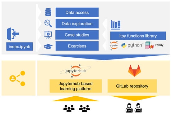
Figure 1.
Overview of Learning Tool for Python main course: general course outline (blue) and the modalities of access (yellow). The notebooks are organized in notebooks on data access, data exploration, case studies and exercises. Learners can either clone the content onto their local machines from a publicly accessible GitLab repository or directly access the JupyterHub-based training platform under https://ltpy.adamplatform.eu (accessed on 16 May 2022). The course starts with the index.ipynb notebook, which introduces learners to the course outline and modality. A notebook with 14 pre-defined functions helps to modularize code and to cater for different levels in programming and coding.
The LTPy course is for learners who have a basic understanding of Earth Observation data and remote sensing but need an overview of data available and a practical introduction on how the data can be accessed, processed and visualized. The course is designed to accommodate learners with different levels of data and coding literacy, from beginners to more advanced users of Python.
2.2. Hosting and Accessibility
The main course is available on a public code repository [], and the thematic module on dust monitoring and forecasting is accessible in the form of an online book (http://dustbook.ltpy.adamplatform.eu/ (accessed on 16 May 2022)) (see Figure 2). Additionally, the notebooks are available through a hosted JupyterHub-based training platform (LTPy main course: https://ltpy.adamplatform.eu/ (accessed on 16 May 2022); thematic module on dust: https://dust.ltpy.adamplatform.eu (accessed on 16 May 2022)), where the required Python environment, package dependencies and data are already available. Course participants are asked to register and create a free account under https://login.ltpy.adamplatform.eu/ (accessed on 16 May 2022).
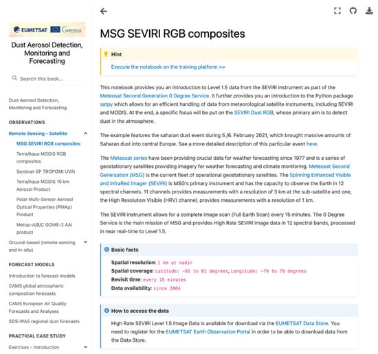
Figure 2.
Screenshot of the Jupyterbook on dust aerosol detection, monitoring and forecasting, which can be accessed via https://dust.trainhub.eumetsat.int/ (accessed on 16 May 2022). The example shows a subpage introducing the Meteosat Second Generation SEVIRI Level 1B data. Each data subpage has on top a link to the executable notebook on a JupyterHub-based training platform and info boxes on ‘basic facts’ and ‘How to access the data’.
Hosted JupyterHub-based training environments provide great flexibility for course participants as well as course providers. Instead of preparing the programming environment on their local machines, training course participants can directly start with the content-based training. For us, as course providers, the hosted option has the advantage that server resources can flexibly be adapted for each training activity, depending on the expected number of participants. With a regular setup, up to 50 concurrent users can access the platform. However, for some larger training events, server resources were adjusted to be able to host up to 100 concurrent users.
2.3. Training Activities and Feedback
Since the start of the Learning Tool for Python on atmospheric composition activities, the Jupyter notebooks have been used in a total of 16 in-person and online training events, and over 1000 learners have been reached (see Table 2). There were three main types of training conducted: (i) training schools, (ii) thematic expert workshops and (iii) short courses. Training schools and thematic expert workshops usually have a duration of several days, while short courses aim to give a lightweight introduction to a specific topic and are usually 1 to 1.5 h long.
Table 2.
Overview of training events, including numbers of training participants for each type of training.
We collected general feedback on the training via a poll conducted with the event audience engagement platform Slido. We asked the following four questions to gather general feedback on the training:
- Q1: Would you recommend the training to a friend or colleague? (Rating from 1 to 5)
- Q2: What did you specifically enjoy or find useful in this session? (Open response)
- Q3: What should we do differently next time? (Open response)
- Q4: What type of information would help you in using a specific dataset? (Multiple choice question)
The overall feedback on the training material was positive. Over 90% (103 responses) would either recommend or highly recommend the training to a colleague or friend (Q1) (see Figure A1 in the Appendix A). Course participants specifically highlighted three aspects as useful (Q2) (see Table A3 in the Appendix A): (i) the practical part of the training activities, including the introduction to Jupyter notebooks; (ii) introduction to atmospheric composition thematic and data; and (iii) the overall course structure, content and organization. A little more than half (54%, n = 57) specifically enjoyed the practical part of the training activities, and two out of five learners (40%, n = 36) highlighted Jupyter notebooks as particularly useful. A total of 92 participants provided suggestions for what could be improved (Q3) (see Table A4 in the Appendix A). By far, the most mentioned suggestion (n = 27) was related to extending the practical training part to include daily assignments and to start workflows from downloading datasets. In total, 196 participants provided a response to Q4 (see Figure A2 in the Appendix A). The two options that would help more than half of the respondents were (i) the provision of examples for basic processing, visualisation and analysis (59%) and (ii) training activities, e.g., short courses, webinars or recorded videos (55%).
3. Guiding Principles for Using Jupyter Notebooks for EO Data Education
During the development of the LTPy notebooks, we applied a set of five guiding principles that helped us to make the notebooks more educational, to cater for different levels of data, thematic and programming expertise and to improve overall navigation to make the training material applicable for instructor-led trainings as well as for self-paced learning. This section outlines these guiding principles.
3.1. Leverage the Literate Programming Paradigm to Make Jupyter Notebooks Educational
The literate programming paradigm is not new and goes back to 1984, when Donald Knuth shared his idea to enrich code with natural language to explain its logic []. Several decades later, notebooks, in fact, became an enabler of the literate paradigm and were designed to facilitate the construction and sharing of computational narratives []. However, several studies which explore the use of Jupyter notebooks among researchers and data scientists discovered that descriptive text in notebooks is (i) unevenly distributed, with most text at the beginning and hardly any text the end, and (ii) resembles more of a collection of loose scripts than a computational narrative. Further, the cell proportion in most notebooks is skewed towards more cells with code than cells with markdown [,]. The importance of annotations and descriptive text, as well as dividing workflows into shorter subsections, increases when notebooks are used for educational purposes []. To see if the notebooks of the LTPy course meet the objective to be educational and well documented, for each notebook we calculated the number of cells in total, number of markdown cells and number of code cells and built the ratio of markdown vs. code cells (see Appendix A Table A5 for notebooks from the main course and Appendix A Table A6 for notebooks from the thematic module). The total number of cells, on average, is 74 for the main course and 55 for the thematic module (Table 3). However, if the exercise notebooks of the thematic module, which tend to have less cells, are not considered, then the total number of cells on average would be 64. The average ratio of markdown vs. code cells is 2.8 for the main course and 3.2 for the thematic module (Table 3). This means that the LTPy notebooks have, on average, three times more markdown cells with descriptive text than cells with code. Figure 3 shows the frequency distribution per markdown/code ratio category. More than half (56%, n = 41) of the notebooks have a markdown/code ratio of 3. Another 21% (n = 15) of the notebooks have a markdown/code ratio of 4. Exercise notebooks tend to have a higher markdown/code ratio than data exploration notebooks or case studies (Table 3).
Table 3.
Average number of total, markdown and code cells for each category of the LTPy main course and of the thematic module. Each entry summarized from Appendix A Table A5 and Table A6.
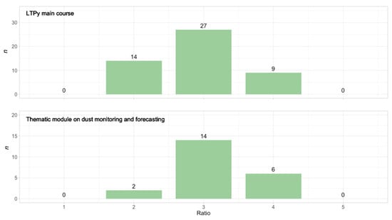
Figure 3.
Frequency plot of number of notebooks per markdown/code ratio category. The ratio category describes the ratio of number of markdown cells vs. number of code cells. For example, a ratio = 3 means that the respective notebooks have three times more annotated cells than code cells. Top: frequency distribution of the notebooks that are part of the LTPy main course (n = 50). Bottom: frequency distribution of notebooks that are part of the thematic module on dust monitoring and forecasting (n = 22). The LTPy main course has one outlier (a notebook with mainly descriptive text on how to access different data) with a ratio of 46.5. This outlier has been removed from the plot.
3.2. Use of Instructional Design Elements
Throughout the course, we leveraged a combination of HTML/Markdown elements that serve as instructional design elements (see Figure 4 and Table 4). These elements improve the look and feel and overall navigation of the course as well as the navigation within a notebook. Each notebook has a navigation pane on top (see Figure 5, box 2). ‘Alert boxes’ help to highlight and cross-reference any prerequisites or related notebooks (see Figure 5, box 1). With the help of anchor links, each notebook has an outline section (table of contents) that allows learners to easily navigate to sub-sections within a notebook (see Figure 5, box 4). Additionally, we make use of backticks (‘…’) to highlight important sections or code in the text of a markdown cell. Backticks change the font to Courier New and highlight the text in grey (see Figure 5, box 3). With these elements, we believe that the notebooks are useful for different training modalities and serve as training material for an instructor-led course, but are also easy to follow and navigate when used for self-paced learning.
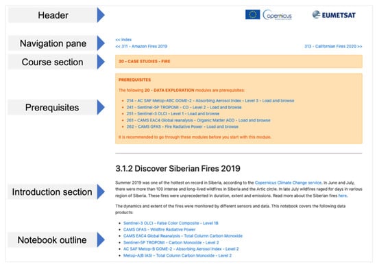
Figure 4.
Example of one case study notebook of the LTPy main course, with several instructional design elements integrated: header, navigation pane, alert boxes (course section and prerequisites), introduction section and notebook outline with anchor links.
Table 4.
Overview of useful HTML/Markdown commands, including their functionality and the objective they fulfill.
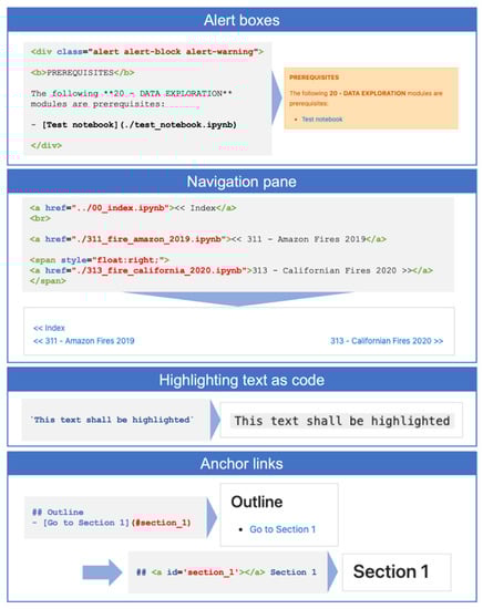
Figure 5.
Overview of HTML/Markdown commands, which were used as instructional design elements, and their rendered output: (i) alert boxes, (ii) navigation pane, (iii) highlighting text as code and (iv) anchor links.
3.3. Follow Best Practices for Scientific Computing
When Jupyter notebooks are used in an educational context, they should not only be conceptualized to teach a specific topic but should also set a good example by following and implementing best practices for scientific computing [,]. Several studies, however, reveal that common practices in notebooks contravene the best practices for scientific computing, such as an out-of-order execution of notebook cells [], poor-quality code [] or code duplication []. While not all best practices defined by Wilson et al., (2014) [] are directly applicable for an educational context, some are to be followed fundamentally, such as bringing imports at the beginning of a notebook, making code style and formatting consistent, using meaningful names for variables and the modularization of content.
An essential part of the LTPy course is a ‘functions’ notebook, which is a collection of 14 pre-defined functions that support the learner with data loading, pre-processing and visualization. This modularization of repetitive code further helps to cater for diverse levels of coding and programming among training course participants. Learners with no or basic Python knowledge learn Python by applying these functions, where only keyword arguments (kwargs) have to be provided. Learners with more Python experience can examine the functions in a separate notebook or build their own functions or code routines in the notebook. External Python scripts or notebooks can be loaded from another notebook with the Jupyter magic command %run (see Table 4 and Figure 6). Once the magic command has been executed, the functions can be applied. The command ‘?function_name’ opens the docstring of the function, which provides learners with a short description of what the function does and the keyword arguments required.
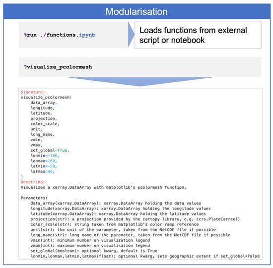
Figure 6.
Magic command (%run) to load content, e.g., functions, from an external script or notebook. Once the command has been executed, the functions can be used in a notebook. The docstring of a function can be called by adding a question mark in front of the function name.
3.4. Take Advantage of the Full Jupyter Ecosystem to Make Content Accessible
A code-sharing platform such as GitHub or GitLab is a common way to share and provide access to notebooks and also offers a built-in rendering of notebooks []. However, the built-in rendering is not ideal, and, for notebooks with an educational purpose, we recommend leveraging the wider ecosystem of Project Jupyter subprojects [] and to make the notebooks available as static but also executable content. ‘nbviewer’, for example, allows you to paste a link to a notebook into a webpage, and it returns a nicely rendered version that can be shared with a unique link. With the help of the Jupyterbook project [], interactive online books can be built based on computational notebooks. We chose to build a Jupyterbook for the thematic module on dust monitoring and forecasting and linked it with a JupyterHub-based training platform in the backend. In this way, learners can browse through the Jupyterbook like they browse through a website. On the top of each Jupyterbook subpage, they can follow a link that opens the executable notebook directly on the JupyterHub-based training platform (see Figure 2). Besides sharing notebooks statically, there are different platforms that offer free compute resources to execute and run notebooks. For example, Binder [] or Kaggle make it possible to open a (collection of) notebook(s) in an executable environment. These are great options if the dependencies of the training environment are not too complex and the data can be retrieved programmatically and is not too large in volume. On the other hand, a self-hosted JupyterHub server offers great flexibility in setting up the training environment and already includes all Python packages and data [,]. This helps to mitigate the challenge of the fragmented landscape of EO data access systems []. The data of the LTPy course are hosted on more than five different data-access systems, and the access modalities range from manually downloading data to downloading data programmatically with an API. Making the data available already on the training platform and providing instructions on how to access data for self-paced learning gives educators flexibility to use the training material for different training formats. We have further discovered that, especially for training participants from regions with limited internet connectivity, the download of large volumes of data is a challenge, but accessing the Jupyter-based training platform is often manageable. On the other hand, a self-hosted JupyterHub server shifts system operation and maintenance responsibility to the training provider, which is often a considerable investment of time and resources [].
3.5. Aim for Reproducibility
The importance of reproducibility increases for notebooks with an educational purpose, especially if the notebooks are used for self-paced learning. To achieve a minimum standard of reproducibility, machine- and human-readable instructions for the data, computing environment and dependencies are required []. Pimentel et al., (2019, 2021) discovered that the reproducibility of notebooks on GitHub is far from ideal and, as a result, defined eight best practices to improve the reproducibility of notebooks. Some are in line with best practices for scientific computing, e.g., (i) abstracting code into functions, classes and modules, and (ii) putting imports at the beginning. Another two practices, (i) paying attention to the bottom of the notebook and (ii) restarting kernel and running all cells, can easily be achieved during the cleaning process of a notebook. In the LTPy course, we further record dependencies, including the package version, in an environment.yml file and provide the data as a zipped tar file for download from an FTP server. However, the growing data volumes of Earth Observation data make this challenging. The data folder for the LTPy main course, for example, has more than 80 GB. We acknowledge that making notebooks reproducible is associated with a considerable amount of extra effort and time investment, but aiming for reproducibility, especially when notebooks are used for training and capacity-building, greatly increases the usability of the notebooks.
4. Discussion
In this paper, we share our experience with using Jupyter notebooks in Earth Observation data education. We adapted five guiding principles, mainly from fields of scientific computing and Jupyter notebooks research, to make the notebooks more educational, reusable and fit for teaching and capacity building. In the following section, we will discuss our reasoning as to why we believe that the five guiding principles introduced in this manuscript are fundamental for EO data education.
Leverage the literate programming paradigm: The literate programming paradigm [] is fundamental for educational notebooks. Currently, the potential for developing rich computational narratives has not been fully unleashed, even though Jupyter notebooks make this easier than ever []. One reason for this may be the considerable time needed to clean up a notebook and to rearrange code and markdown cells into a coherent workflow and narrative. The results from Rule et al., (2018), who analyzed more than one million notebooks hosted on Github, revealed that one out of four notebooks had no text at all, and those who had text had hardly more than 1000 words. The results from Quaranta et al., (2022) show a median text/code ratio of 0.4 (7/19), indicating that the ~1000 notebooks analyzed in the study had 2.7 times more code than text []. In comparison, the text/code ratio of the LTPy notebooks seems exceptional. Their text/code ratio is exactly reversed, having an average text/code ratio of 3. Even though there are no defined minimum standards for notebooks, we could conclude that a text/code ratio of at least two (twice as much text cells than code cells) could be an indication of the literate programming paradigm and meeting the criteria of being ‘educational’.
Use of instructional design elements: This guiding principle originates mainly from the need to make the training material coherent and easy to navigate for both self-paced learning and during an instructor-led training session. We are not aware of any minimum standards concerning instructional design elements in Jupyter notebooks that have been defined so far. Hence, this manuscript can be considered as a starting point to share one approach and practical implementation examples on how UX design features can be leveraged to increase the look and feel, quality and overall navigation of notebooks. An important next step would be to collect feedback on whether the instructional design patterns implemented in the LTPy fulfil their objective.
Take advantage of the full Project Jupyter ecosystem to make content accessible: Johnson (2020) describes the benefits and pitfalls of using Jupyter notebooks in an academic classroom and highlights, for example, that the client–server model upon which Jupyter notebooks are based is often already a hurdle for novice users []. Accessing and processing EO data that is browser- or web-based is a ‘paradigm-change’ for EO data users, especially as the majority still process large volumes of EO data locally [,]. Hence, conducting training based on Project Jupyter tools not only supports EO data users in their current needs, but also helps familiarize them with future data processing interfaces. The web interface JupyterLab, in particular, is often seen as the ‘next-generation’ user interface for conducting data science [,]. We believe that this will also be the case for Earth Observation data science. Many Earth Observation platforms and EO cloud-based services already offer a JupyterLab web interface to access and process EO data. Hence, computational notebooks can be considered as a facilitator for the paradigm ‘bringing users to the data’ and the transition to cloud-based services for Big Earth data [,].
Follow best practices for scientific computing: Using Jupyter notebooks in an educational context amplifies the responsibility to develop high-quality notebooks that follow best practices on scientific computing [] and the use of Jupyter notebooks. Despite an exponential growth of Jupyter notebooks on GitHub in recent years, most notebooks fall short in terms of quality and following common best practices. One reason could be that best practices and practical implementation examples are not well known and the pitfalls of Jupyter notebooks are not well understood. Even though not all best practices for scientific computing and the use of Jupyter notebooks are directly applicable to an educational context, the two we consider fundamental are the modularization of content and importing libraries at the beginning. The latter is relatively easy to implement with no additional effort and seems to be adopted in most cases []. Modularizing content, e.g., functions, can be time-consuming, especially to make the functions applicable to different types of EO data products. From our experience, the time investment pays off, as from an educational perspective, the modularization of functions not only follows best practices for scientific computing, but also helps to cater for different levels of coding and programming expertise.
Aim for reproducibility: Being reproducible is a big claim, which we do not dare to make. For this reason, as a guiding principle, we advocate to ‘aim’ for reproducibility when developing Jupyter notebooks in an educational context. The minimum reproducibility aspects that should be followed in an educational context are to re-run notebooks from top to bottom, to clean any empty cells and to make the processing environment including data reproducible. It seems that there is a misconception that content is automatically reproducible when made available as a Jupyter notebook. The study by Pimentel et al., (2019, 2021), however, revealed that only a quarter of the notebooks available on Github can be re-executed. In the study by Quaranta et al., (2022), a surprisingly high percentage of the notebooks analyzed on Kaggle had a linear execution order. They argue that this best practice is enforced by Kaggle, and that the ‘execute all’ command is part of the commit process. In the Jupyter ecosystem, this process needs to be invoked manually. One suggestion for future developments could be that best practices are automatically integrated in the ecosystem. For example, when a notebook is committed to a code sharing platform, a cleaning of empty cells and an execution of cells from top to bottom is automatically invoked.
5. Conclusions and Future Outlook
The increase in open Earth Observation data and the emergence of cloud-based services require stronger efforts in training EO data users to ensure continued EO data uptake and use. By sharing our experience and guiding principles on how to make notebooks more educational, we hope we can contribute to increasing the overall quality and usability of Jupyter notebooks, especially when these are used in an educational context. Current best practices focus on the general use of notebooks among data scientists, but more research and practical examples from the community on how to make notebooks more educational are required. We see two areas of future developments as relevant. First, we need a better understanding of notebook users, the benefits they seek and the challenges they face when starting to use notebooks, especially in application domains where the use of Jupyter notebooks is growing, such as in the field of Earth Observation research. Further, we need an evaluation of whether the instructional design elements that were shared in this manuscript meet their purpose of improving the navigation through the training material. Second, we believe that time is the main the reason why best practices related to scientific computing or reproducibility are often not followed. Some best practices could be invoked by developing, e.g., a Jupyter extension, which re-executes a notebook from top to bottom and removes empty code cells before it is committed.
Author Contributions
Conceptualization, J.W. and F.F.; writing—original draft preparation, J.W.; writing—review and editing, J.W., F.F., S.M., S.S., B.S. and J.B. All authors have read and agreed to the published version of the manuscript.
Funding
This work has partially been funded under the framework of EUMETSAT/Copernicus contract No. 19/218240. Open Access funding provided by the Open Access Publication Fund of Philipps-Universität Marburg with support of the Deutsche Forschungsgemeinschaft (DFG, German Research Foundation).
Data Availability Statement
The data presented in this study are available on request from the corresponding author. The data are not publicly available.
Acknowledgments
We thank all the colleagues at EUMETSAT and participants at various training events whose feedback fundamentally helped to improve the LTPy course.
Conflicts of Interest
The authors declare no conflict of interest.
Appendix A
Table A1.
Overview of satellite- and model-based products featured in the LTPy main course.
Table A1.
Overview of satellite- and model-based products featured in the LTPy main course.
| Satellite-Based Products | ||
|---|---|---|
| Satellite | Instrument | Data Product(s) |
| Metop series (consists of three satellites: Metop-A, -B, -C) | Global Ozone Monitoring Experiment-2 (GOME-2) | Absorbing Aerosol Index (AAI) Absorbing Aerosol Height (AAH) Tropospheric Nitrogen Dioxide (NO2) |
| Metop series (consists of three satellites: Metop-A, -B, -C) | Infrared Atmospheric Sounding Interferometer (IASI) | Carbon Monoxide Ammonia (NH3) |
| Sentinel-5 Precursor (Sentinel-5P) | TROPOspheric Monitoring Instrument (TROPOMI) | Carbon Monoxide (CO) Ultraviolet Aerosol Index (UVAI) |
| Sentinel-3 | Ocean and Land Colour Instrument (OLCI) | Level 1 RGB True- and False-Color composites |
| Sentinel-3 | Sea and Land Surface Temperature Radiometer (SLSTR) | Fire Radiative Power (FRP) Aerosol Optical Depth (AOD) |
| Metop series (consists of three satellites: Metop-A, -B, -C) | GOME-2, IASI, Advance Very High Resolution Radiometer (AVHRR) | Polar Multi-Sensor Aerosol Optical Properties (PMAp) Aerosol Optical Depth (AOD) |
| Model-based products | ||
| Operational service | Product type | Data variable(s) |
| Copernicus Atmospheric Monitoring Service (CAMS) | Global Fire Assimilation System (GFAS) | Fire Radiative Power (FRP) |
| Copernicus Atmospheric Monitoring Service (CAMS) | Global reanalysis (EAC4) | Organic Matter Aerosol Optical Depth (OMAOD) Ozone (O3) |
| Copernicus Atmospheric Monitoring Service (CAMS) | Global atmospheric composition forecasts | Dust Aerosol Optical Depth |
| Copernicus Atmospheric Monitoring Service (CAMS) | European air quality forecasts | Dust concentration Nitrogen Dioxide (NO2) |
| Copernicus Emergency Management Service (CEMS) | Global ECMWF Fire Forecast (GEFF) | Fire Weather Index (FWI) |
Table A2.
Overview of satellite-, model- and ground-based products featured in the thematic module on dust monitoring and forecasting.
Table A2.
Overview of satellite-, model- and ground-based products featured in the thematic module on dust monitoring and forecasting.
| Satellite-Based Products | ||
| Satellite | Instrument | Data Product(s) |
| Metop series (consists of three satellites: Metop-A, -B, -C) | Global Ozone Monitoring Experiment-2 (GOME-2) | Absorbing Aerosol Index (AAI) |
| Sentinel-5 Precursor (Sentinel-5P) | TROPOspheric Monitoring Instrument (TROPOMI) | Ultraviolet Aerosol Index (UVAI) |
| Metop series (consists of three satellites: Metop-A, -B, -C) | GOME-2, IASI, Advanced Very High Resolution Radiometer (AVHRR) | Polar Multi-Sensor Aerosol Optical Properties (PMAp) Aerosol Optical Depth (AOD) |
| Meteosat Second Generation | Spinning Enhance Visible and InfraRed Image (SEVIRI) | Level 1 RGB True- and False-Color composites |
| Terra and Aqua | Moderate Resolution Imaging Spectroradiometer (MODIS) | Level 1 RGB True- and False- Color composites Aerosol Optical Depth (AOD) |
| Model-based products | ||
| Operational service | Product type | Data variable(s) |
| Copernicus Atmosphere Monitoring Service (CAMS) | Global atmospheric composition forecasts | Dust Aerosol Optical Depth |
| Copernicus Atmosphere Monitoring Service (CAMS) | European air quality forecasts | Dust concentration |
| Barcelona Dust Regional Center | Regional dust forecasts for Northern Africa, Middle East and Europe | Dust Aerosol Optical Depth |
| Ground-based products | ||
| Data service | Ground-based sensor | Data variable(s) |
| Aerosol Robotic NETwork | Sun photometer | Aerosol Optical Depth Angstrom Exponent Coefficient |
| European Aerosol Research Lidar Network (EARLINET) | Lidar | Vertical backscatter profile |
| European Environment Agency (EEA) Air Quality Data | Particulate Matter Sensor | Particulate Matter 2.5 (PM2.5) Particulate Matter 10 (PM10) |
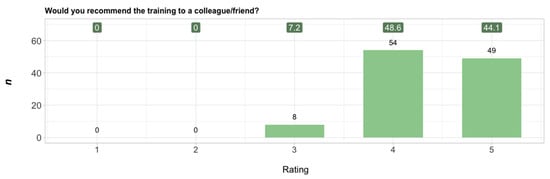
Figure A1.
Rating by training participants (n = 111) whether they would recommend the training to a friend/colleague. Rating levels were from 1 (low) to 5 (high). Bars indicate absolute numbers, labels on top indicate relative frequencies in %.
Table A3.
Categories built based on the open response question ‘What did you specifically enjoy or find useful in the session?” (n = 105). Note: some responses could be categorized into two categories.
Table A3.
Categories built based on the open response question ‘What did you specifically enjoy or find useful in the session?” (n = 105). Note: some responses could be categorized into two categories.
| Category | n | % | Example Responses |
|---|---|---|---|
| Practical session in general, including introduction to Jupyter notebooks | 57 | 54.3 |
|
| Introduction to atmospheric composition thematic and data, including scientific lectures | 36 | 34.3 |
|
| Course structure, content and organization | 23 | 21.9 |
|
Table A4.
Categories of responses to the question ‘What should we do differently next time?’ (n = 92). Categories on the left have four or more mentions, with the first category (Extension of practical training part) being by far the most mentioned suggestion (n = 27). Others had four or five mentions. Categories on the right were mentioned less than four times but are considered as useful suggestions.
| Categories with Four or More Mentions | Categories with Less than Four Mentions |
|---|---|
| Extension of the practical training, including daily assignments and start workflows from downloading datasets More breaks during the practical training, including more time for introducing the Jupyter-based training platform and explaining Python code principles Preference for in-person training More scientific depth and inter- connections of the atmospheric composition topic | Provide more references to books, articles and data documentation Provide presentations and practical training content in beforehand More time for Q&A and provide written answers to questions Provide a space for offline discussions after the training course Offer separate introduction to Python/Jupyter notebooks/xarray Inform about the level of difficulty of the practical part in beforehand Provide more trainers for practical part |
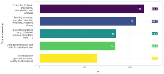
Figure A2.
Responses to the question ‘What type of information would help you in using a specific dataset?’ (n = 196). Bars indicate absolute numbers, labels on the right indicate relative frequencies in %.
Table A5.
Overview of notebooks that are part of the LTPy main course and, for each notebook, the number of cells in total, number of markdown cells, number of code cells and the markdown/code ratio are listed.
Table A5.
Overview of notebooks that are part of the LTPy main course and, for each notebook, the number of cells in total, number of markdown cells, number of code cells and the markdown/code ratio are listed.
| No. | Notebook Title | # of Cells (Total) | No. of Cells (Markdown) | No. of Cells (Code) | Ratio (Markdown/Code) |
|---|---|---|---|---|---|
| Section I—Data access | |||||
| 1.1 | Atmospheric composition data—Overview and data access | 95 | 93 | 2 | 46.5 |
| 1.2 | WEkEO Harmonized data access (HDA) API | 55 | 40 | 15 | 2.7 |
| Section II—Data exploration | |||||
| 2.1.1 | AC SAF Metop-A GOME-2—Tropospheric NO2—Level 2—Load and browse | 52 | 40 | 12 | 3.3 |
| 2.1.2 | AC SAF Metop-A/B GOME-2—Tropospheric NO2—Level 2—Pre-process | 72 | 52 | 20 | 2.6 |
| 2.1.3 | AC SAF Metop-A/B GOME-2—Tropospheric NO2- Level 3—Load and browse | 38 | 29 | 9 | 3.2 |
| 2.1.4 | AC SAF Metop-A/B/C GOME-2—Absorbing Aerosol Index—Level 3—Load and browse | 54 | 39 | 15 | 2.6 |
| 2.1.5 | AC SAF Metop-A/B/C GOME-2—Absorbing Aerosol Height—Level 2—Load and browse | 59 | 46 | 13 | 3.5 |
| 2.2.1 | Polar Multi-Sensor Aerosol Optical Properties (PMAp)—Aerosol Optical Depth—Level 2—Load and browse | 41 | 32 | 9 | 3.6 |
| 2.3.1 | Metop-A/B IASI—Ammonia (NH3)—Level 2—Load and browse | 55 | 40 | 15 | 2.7 |
| 2.3.2 | Metop-A/B IASI—Carbon Monoxide—Level 2—Load and browse | 68 | 48 | 20 | 2.4 |
| 2.4.1 | Sentinel-5P TROPOMI—Carbon Monoxide—Level 2—Load and browse | 47 | 35 | 12 | 2.9 |
| 2.4.2 | Sentinel-5P TROPOMI—Ultraviolet Aerosol Index—Level 2—Load and browse | 40 | 32 | 8 | 4.0 |
| 2.5.1 | Sentinel-3 OLCI—Radiances—Level 1—Load and browse | 77 | 52 | 25 | 2.1 |
| 2.5.2 | Sentinel-3 SLSTR NRT—Fire Radiative Power (FRP)—Level 2—Load and browse | 84 | 56 | 28 | 2.0 |
| 2.5.3 | Sentinel-3 SLSTR NRT—Aerosol Optical Depth (AOD)—Level 2—Load and browse | 31 | 25 | 6 | 4.2 |
| 2.6.1 | CAMS Global reanalysis (EAC4)—Organic Matter Aerosol Optical Depth—Load and browse | 61 | 42 | 19 | 2.2 |
| 2.6.2 | CAMS Global Fire Assimilation System (GFAS)—Fire Radiative Power—Load and browse | 33 | 25 | 8 | 3.1 |
| 2.6.3 | CAMS Global Forecast—Dust Aerosol Optical Depth—Load and browse | 60 | 43 | 17 | 2.5 |
| 2.6.4 | CAMS European air quality forecast—Dust Concentration—Load and browse | 64 | 46 | 18 | 2.6 |
| 2.6.5 | European air quality forecast—Nitrogen Dioxide—Load and browse | 63 | 45 | 18 | 2.5 |
| 2.7.1 | CEMS Global ECMWF Fire Forecast—Fire Weather Index—Load and browse | 87 | 63 | 24 | 2.6 |
| 2.7.2 | CEMS Global ECMWF Fire Forecast—Fire Weather Index—Harmonized Danger Classes | 36 | 29 | 7 | 4.1 |
| 2.7.3 | CEMS Global ECMWF Fire Forecast—Fire Weather Index—Custom Danger Classes | 61 | 41 | 20 | 2.1 |
| Section III—Case studies | |||||
| 3.1.0 | Case study—Siberian fires 2021—Multi-data | 110 | 77 | 33 | 2.3 |
| 3.1.1 | Case study—Amazon fires 2019—Multi-data | 73 | 50 | 23 | 2.2 |
| 3.1.2 | Case study—Siberian fires 2019—Multi-data | 119 | 82 | 37 | 2.2 |
| 3.1.3 | Case study—Californian fires 2020—Multi-data | 160 | 113 | 47 | 2.4 |
| 3.1.4 | Case study—Chernobyl fires 2020—Sentinel-3 SLSTR NRT—Fire Radiative Power | 82 | 56 | 26 | 2.2 |
| 3.1.5 | Case study—Californian fires 2020—Sentinel-3 SLSTR NRT—Fire Radiative Power | 81 | 55 | 26 | 2.1 |
| 3.1.6 | Case study—Californian fires 2020—Sentinel-3 SLSTR NRT—Aerosol Optical Depth | 31 | 25 | 6 | 4.2 |
| 3.1.7 | Case study—Indonesian fires 2015—Multi-data | 148 | 106 | 42 | 2.5 |
| 3.1.8 | Case study—Indonesian fires 2020—Multi-data | 93 | 67 | 26 | 2.6 |
| 3.1.9 | Case study—Portugal fires 2020—Multi-data | 205 | 145 | 60 | 2.4 |
| 3.2.1 | Case study—Map and time-series analysis—AC SAF Metop-A/B GOME-2—Tropospheric NO2 | 43 | 33 | 10 | 3.3 |
| 3.2.2 | Case study—Produce gridded dataset—AC SAF Metop-A/B GOME-2—Tropospheric NO2 | 71 | 51 | 20 | 2.6 |
| 3.2.3 | Case study—Create an anomaly map—Europe—AC SAF Metop-A/B GOME-2—Tropospheric NO2 | 122 | 83 | 39 | 2.1 |
| 3.2.4 | Case study—Time-series analysis—Europe—AC SAF Metop-A/B GOME-2—Tropospheric NO2 | 63 | 45 | 18 | 2.5 |
| 3.2.5 | Case study—Create an anomaly map—Europe—Sentinel-5P TROPOMI—Tropospheric NO2 | 57 | 41 | 16 | 2.6 |
| 3.2.6 | Case study—Time-series analysis—Europe—Sentinel-5P TROPOMI—Tropospheric NO | 58 | 44 | 14 | 3.1 |
| 3.3.1 | Case study—Antarctic ozone hole 2019—Multi-data | 76 | 51 | 25 | 2.0 |
| 3.3.2 | Case study—Antarctic ozone hole 2019—CAMS animation | 31 | 24 | 7 | 3.4 |
| 3.3.3 | Case study—Antarctic ozone hole 2020—AC SAF Metop-A/B/C GOME-2 Level 2 | 86 | 63 | 23 | 2.7 |
| 3.3.4 | Case study—Arctic ozone hole 2020—Metop-A/B/C IASI Level 2 | 84 | 63 | 21 | 3.0 |
| 3.3.5 | Case study—Arctic ozone hole 2020—CAMS Reanalysis (EAC4) | 36 | 28 | 8 | 3.5 |
| Section IV—Exercises | |||||
| 4.1.1 | Exercise—Sentinel-5P TROPOMI—Carbon Monoxide—Level 2 | 82 | 62 | 20 | 3.0 |
| 4.2.1 | Exercise—Sentinel-3 OLCI—Radiances—Level 1 | 97 | 73 | 24 | 3.0 |
| 4.2.2 | Exercise—Sentinel-3 SLSTR NRT—Fire Radiative Power | 85 | 63 | 22 | 3.0 |
| 4.2.3 | Exercise—Sentinel-3 SLSTR NRT—Aerosol Optical Depth | 54 | 43 | 11 | 4.0 |
| 4.3.1 | Exercise—CAMS Global Reanalysis (EAC4)—Total Column Carbon Monoxide | 59 | 47 | 12 | 4.0 |
| 4.4.1 | Exercise—AC SAF Metop-A/B/C GOME-2—Ozone | 125 | 95 | 30 | 3.0 |
| 4.4.2 | Exercise—Metop-A/B/C IASI—Ozone | 107 | 80 | 27 | 3.0 |
Table A6.
Overview of notebooks that are part of the thematic module on dust monitoring and forecasting and for each notebook the number of cells in total, number of markdown cells, number of code cells and the markdown/code ratio is listed.
Table A6.
Overview of notebooks that are part of the thematic module on dust monitoring and forecasting and for each notebook the number of cells in total, number of markdown cells, number of code cells and the markdown/code ratio is listed.
| No. | Notebook Title | # of Cells (Total) | No. of Cells (Markdown) | No. of Cells (Code) | Ratio (Markdown/Code) |
|---|---|---|---|---|---|
| Section I—Observations—Satellite data | |||||
| 1.1.1 | Meteosat Second Generation SEVIRI—True color and dust RGB—Level 1 | 101 | 74 | 27 | 2.7 |
| 1.1.2 | MODIS—True color and dust RGB—Level 1B | 80 | 60 | 20 | 3.0 |
| 1.1.3 | Sentinel-5P TROPOMI—Ultraviolet Aerosol Index—Level 2 | 48 | 36 | 12 | 3.0 |
| 1.1.4 | MODIS—10 km aerosol product—Level 2 | 49 | 38 | 11 | 3.5 |
| 1.1.5 | Polar Multi-Sensor Aerosol Optical Properties (PMAp) Product—Aerosol Optical Depth—Level 2 | 50 | 39 | 11 | 3.5 |
| 1.1.6 | Metop-ABC GOME-2—Absorbing Aerosol Index—Level 3 | 64 | 49 | 15 | 3.3 |
| Section I—Observations—Ground-based data | |||||
| 1.2.1 | AERONET—AErosol RObotic NETwork | 67 | 53 | 14 | 3.8 |
| 1.2.2 | European Aerosol Research Lidar Network (EARLINET)—Backscatter profiles | 37 | 30 | 7 | 4.3 |
| 1.2.3 | European Environment Agency Air Quality Data | 48 | 36 | 12 | 3.0 |
| Section II—Model forecasts | |||||
| 2.1 | CAMS global atmospheric composition forecast—Dust Aerosol Optical Depth | 74 | 53 | 21 | 2.5 |
| 2.2 | CAMS European Air Quality Forecasts—Dust concentration | 74 | 54 | 20 | 2.7 |
| 2.3 | WMO SDS-WAS MONARCH—Dust Forecast | 46 | 34 | 12 | 2.8 |
| Section III—Practical case study | |||||
| 3.1 | Exercise 01 Exercise 01—Solution | 21 77 | 17 56 | 4 21 | 4.3 2.7 |
| 3.2 | Exercise 02 Exercise 02—Solution | 30 73 | 23 52 | 7 21 | 3.3 2.5 |
| 3.3 | Exercise 03 Exercise 03—Solution | 31 66 | 24 49 | 7 17 | 3.4 2.9 |
| 3.4 | Exercise 04 Exercise 04—Solution | 28 76 | 22 54 | 6 22 | 3.7 2.5 |
| 3.5 | Exercise 05 Exercise 05—Solution | 21 57 | 17 43 | 4 14 | 4.3 3.1 |
References
- Wagemann, J.; Siemen, S.; Seeger, B.; Bendix, J. Users of Open Big Earth Data—An Analysis of the Current State. Comput. Geosci. 2021, 157, 104916. [Google Scholar] [CrossRef]
- Price Waterhouse Coopers (PWC). Main Trends and Challenges in the Space Sector; PWC: Neuilly-sur-Seine, France, 2020. [Google Scholar]
- Hebden, S. Plans for a New Wave of European Satellites. 2020. [Google Scholar]
- European Organisation for the Exploitation of Meteorological Satellites Meteosat Series|EUMETSAT. Available online: https://www.eumetsat.int/our-satellites/meteosat-series?sjid=future (accessed on 12 February 2022).
- Masek, J.G.; Wulder, M.A.; Markham, B.; McCorkel, J.; Crawford, C.J.; Storey, J.; Jenstrom, D.T. Landsat 9: Empowering Open Science and Applications through Continuity. Remote Sens. Environ. 2020, 248, 111968. [Google Scholar] [CrossRef]
- National Aeronautics and Space Administration Landsat NeXt|Landsat Science. Available online: https://landsat.gsfc.nasa.gov/satellites/landsat-next/ (accessed on 12 February 2022).
- Bernd, A.; Braun, D.; Ortmann, A.; Ulloa-Torrealba, Y.Z.; Wohlfart, C.; Bell, A. More than Counting Pixels—Perspectives on the Importance of Remote Sensing Training in Ecology and Conservation. Remote Sens. Ecol. Conserv. 2017, 3, 38–47. [Google Scholar] [CrossRef] [Green Version]
- Miguel-Lago, M. Towards an Innovative Strategy for Skills Development and Capacity Building in the Space Geoinformation Sector Supporting Copernicus User Uptake: Deliverable 1.6—Space/Geospatial Sector Skills Strategy; EO4GEO: Genova, Italy, 2019. [Google Scholar]
- Hodam, H.; Rienow, A.; Jürgens, C. Bringing Earth Observation to Schools with Digital Integrated Learning Environments. Remote Sens. 2020, 12, 345. [Google Scholar] [CrossRef] [Green Version]
- European Space Agency ESA—European Space Education Resource Office. Available online: https://www.esa.int/Education/Teachers_Corner/European_Space_Education_Resource_Office (accessed on 16 May 2022).
- Friedrich Schiller Universität Jena. Welcome to EO College—EO College. Available online: https://eo-college.org/welcome (accessed on 16 May 2022).
- Davies, A.; Hooley, F.; Causey-Freeman, P.; Eleftheriou, I.; Moulton, G. Using Interactive Digital Notebooks for Bioscience and Informatics Education. PLoS Comput. Biol. 2020, 16, e1008326. [Google Scholar] [CrossRef]
- Kim, B.; Henke, G. Easy-to-Use Cloud Computing for Teaching Data Science. J. Stat. Data Sci. Educ. 2021, 29, S103–S111. [Google Scholar] [CrossRef]
- Bauer, T.; Immitzer, M.; Mansberger, R.; Vuolo, F.; Márkus, B.; Wojtaszek, M.V.; Földváry, L.; Szablowska-Midor, A.; Kozak, J.; Oliveira, I.; et al. The Making of a Joint E-Learning Platform for Remote Sensing Education: Experiences and Lessons Learned. Remote Sens. 2021, 13, 1718. [Google Scholar] [CrossRef]
- Maggioni, V.; Girotto, M.; Habib, E.; Gallagher, M.A. Building an Online Learning Module for Satellite Remote Sensing Applications in Hydrologic Science. Remote Sens. 2020, 12, 3009. [Google Scholar] [CrossRef]
- Perkel, J.M. Why Jupyter Is Data Scientists’ Computational Notebook of Choice. Nature 2018, 563, 145–146. [Google Scholar] [CrossRef] [Green Version]
- Perkel, J.M. Ten Computer Codes That Transformed Science. Nature 2021, 589, 344–348. [Google Scholar] [CrossRef]
- Rule, A.; Tabard, A.; Hollan, J.D. Exploration and Explanation in Computational Notebooks. In Proceedings of the 2018 CHI Conference on Human Factors in Computing Systems, Montreal, QC, Canada, 21–26 April 2018; ACM: Montreal, QC, Canada, 2018; pp. 1–12. [Google Scholar]
- Lau, S.; Drosos, I.; Markel, J.M.; Guo, P.J. The Design Space of Computational Notebooks: An Analysis of 60 Systems in Academia and Industry. In Proceedings of the 2020 IEEE Symposium on Visual Languages and Human-Centric Computing (VL/HCC), Dunedin, New Zealand, 10–14 August 2020; IEEE: Dunedin, New Zealand, 2020; pp. 1–11. [Google Scholar]
- Pimentel, J.F.; Murta, L.; Braganholo, V.; Freire, J. A Large-Scale Study About Quality and Reproducibility of Jupyter Notebooks. In Proceedings of the 2019 IEEE/ACM 16th International Conference on Mining Software Repositories (MSR), Montreal, QC, Canada, 25–31 May 2019; IEEE: Montreal, QC, Canada, 2019; pp. 507–517. [Google Scholar]
- Pimentel, J.F.; Murta, L.; Braganholo, V.; Freire, J. Understanding and Improving the Quality and Reproducibility of Jupyter Notebooks. Empir. Softw. Eng. 2021, 26, 65. [Google Scholar] [CrossRef] [PubMed]
- Chattopadhyay, S.; Prasad, I.; Henley, A.Z.; Sarma, A.; Barik, T. What’s Wrong with Computational Notebooks? Pain Points, Needs, and Design Opportunities. In Proceedings of the 2020 CHI Conference on Human Factors in Computing Systems, Honolulu, HI, USA, 25–30 April 2020; ACM: Honolulu, HI, USA, 2020; pp. 1–12. [Google Scholar]
- Engelberger, F.; Galaz-Davison, P.; Bravo, G.; Rivera, M.; Ramírez-Sarmiento, C.A. Developing and Implementing Cloud-Based Tutorials That Combine Bioinformatics Software, Interactive Coding, and Visualization Exercises for Distance Learning on Structural Bioinformatics. J. Chem. Educ. 2021, 98, 1801–1807. [Google Scholar] [CrossRef]
- Clarke, D.J.B.; Jeon, M.; Stein, D.J.; Moiseyev, N.; Kropiwnicki, E.; Dai, C.; Xie, Z.; Wojciechowicz, M.L.; Litz, S.; Hom, J.; et al. Appyters: Turning Jupyter Notebooks into Data-Driven Web Apps. Patterns 2021, 2, 100213. [Google Scholar] [CrossRef]
- Lasser, J.; Manik, D.; Silbersdorff, A.; Säfken, B.; Kneib, T. Introductory Data Science across Disciplines, Using Python, Case Studies, and Industry Consulting Projects. Teach. Stat. 2021, 43, S190–S200. [Google Scholar] [CrossRef]
- Boscoe, B.M.; Pasquetto, I.V.; Golshan, M.S.; Borgman, C.L. Using the Jupyter Notebook as a Tool for Open Science: An Empirical Study. In Proceedings of the 2017 ACM/IEEE Joint Conference on Digital Libraries (JCDL), Toronto, ON, Canada, 19–23 June 2017. [Google Scholar]
- Camara, G.S.; Camboim, S.P.; Bravo, J.V.M. Using Jupyter Notebooks for Viewing and Analysing Geospatial Data: Two Examples for Emotional Maps and Education Data. Int. Arch. Photogramm. Remote Sens. Spatial Inf. Sci. 2021, XLVI-4/W2-2021, 17–24. [Google Scholar] [CrossRef]
- Committee on Earth Observation Satellites. Jupyter Notebooks for Capacity Development Webinar|CEOS. Available online: https://ceos.org/meetings/jupyter-notebooks-for-capacity-development-webinar/ (accessed on 10 February 2022).
- Granger, B.E.; Perez, F. Jupyter: Thinking and Storytelling with Code and Data. Comput. Sci. Eng. 2021, 23, 7–14. [Google Scholar] [CrossRef]
- Jupyter, P.; Bussonnier, M.; Forde, J.; Freeman, J.; Granger, B.; Head, T.; Holdgraf, C.; Kelley, K.; Nalvarte, G.; Osheroff, A.; et al. Binder 2.0—Reproducible, Interactive, Sharable Environments for Science at Scale. In Proceedings of the 17th Python in Science Conference (SciPy 2018), Austin, TX, USA, 9–15 July 2018; pp. 113–120. [Google Scholar]
- Rule, A.; Birmingham, A.; Zuniga, C.; Altintas, I.; Huang, S.-C.; Knight, R.; Moshiri, N.; Nguyen, M.H.; Rosenthal, S.B.; Pérez, F.; et al. Ten Simple Rules for Writing and Sharing Computational Analyses in Jupyter Notebooks. PLoS Comput. Biol. 2019, 15, e1007007. [Google Scholar] [CrossRef] [PubMed]
- Quaranta, L.; Calefato, F.; Lanubile, F. Eliciting Best Practices for Collaboration with Computational Notebooks. Proc. ACM Hum. Comput. Interact. 2022, 6, 1–41. [Google Scholar] [CrossRef]
- Johnson, J.W. Benefits and Pitfalls of Jupyter Notebooks in the Classroom. In Proceedings of the 21st Annual Conference on Information Technology Education, Virtual, 7–9 October 2020; ACM: New York, NY, USA, 2020; pp. 32–37. [Google Scholar]
- Wagemann, J.; Szeto, S.; Mantovani, S.; Fierli, F. Learning Tool for Python on Atmospheric Composition. J. Open Source Educ. 2022. under review. [Google Scholar]
- Knuth, D.E. Literate Programming. Comput. J. 1984, 27, 97–111. [Google Scholar] [CrossRef] [Green Version]
- Wilson, G.; Aruliah, D.A.; Brown, C.T.; Chue Hong, N.P.; Davis, M.; Guy, R.T.; Haddock, S.H.D.; Huff, K.D.; Mitchell, I.M.; Plumbley, M.D.; et al. Best Practices for Scientific Computing. PLoS Biol. 2014, 12, e1001745. [Google Scholar] [CrossRef] [PubMed] [Green Version]
- Wang, J.; Kuo, T.; Li, L.; Zeller, A. Assessing and Restoring Reproducibility of Jupyter Notebooks. In Proceedings of the 35th IEEE/ACM International Conference on Automated Software Engineering, Virtual, 21–25 December 2020; pp. 138–149. [Google Scholar]
- Koenzen, A.P.; Ernst, N.A.; Storey, M.-A.D. Code Duplication and Reuse in Jupyter Notebooks. In Proceedings of the 2020 IEEE Symposium on Visual Languages and Human-Centric Computing (VL/HCC), Dunedin, New Zealand, 10–14 August 2020; IEEE: Dunedin, New Zealand, 2020; pp. 1–9. [Google Scholar]
- Executable Books Community. Jupyter Book; Zenodo/CERN: Geneva, Switzerland, 2020. [Google Scholar]
- Wagemann, J.; Siemen, S.; Seeger, B.; Bendix, J. A User Perspective on Future Cloud-Based Services for Big Earth Data. Int. J. Digit. Earth 2021, 14, 1758–1774. [Google Scholar] [CrossRef]
- Echterhoff, J.; Wagemann, J.; Lieberman, J. Earth Observation Cloud Platform Concept Development Study Report; Open Geospatial Consortium, Inc.: Arlington, VA, USA, 2021. [Google Scholar]
Publisher’s Note: MDPI stays neutral with regard to jurisdictional claims in published maps and institutional affiliations. |
© 2022 by the authors. Licensee MDPI, Basel, Switzerland. This article is an open access article distributed under the terms and conditions of the Creative Commons Attribution (CC BY) license (https://creativecommons.org/licenses/by/4.0/).