
Drone-Based Bathymetry Modeling for Mountainous Shallow Rivers in Taiwan Using Machine Learning


Abstract
:
1. Introduction
- (1)
- using UAV with multispectral camera to capture images and surveyed cross-section under shallow bathymetry conditions;
- (2)
- applying a ML algorithm to establish a water depth retrieval model for the rivers of Taiwan’s mountain area, which has yet been found in related studies;
- (3)
- encrypting the established model to Python-based program for further application, which can be used to simulate water depth for the shallow river or near-shore areas that are not easily measured under similar conditions as this study, where the water depth could be estimated by multispectral sensor mounted on the UAV.
2. Materials and Methods
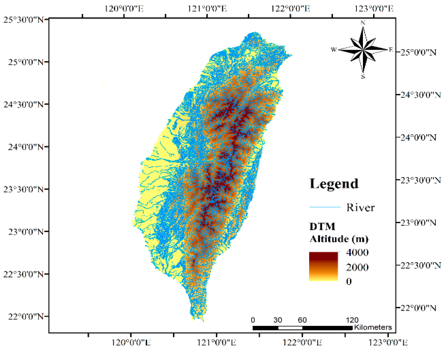
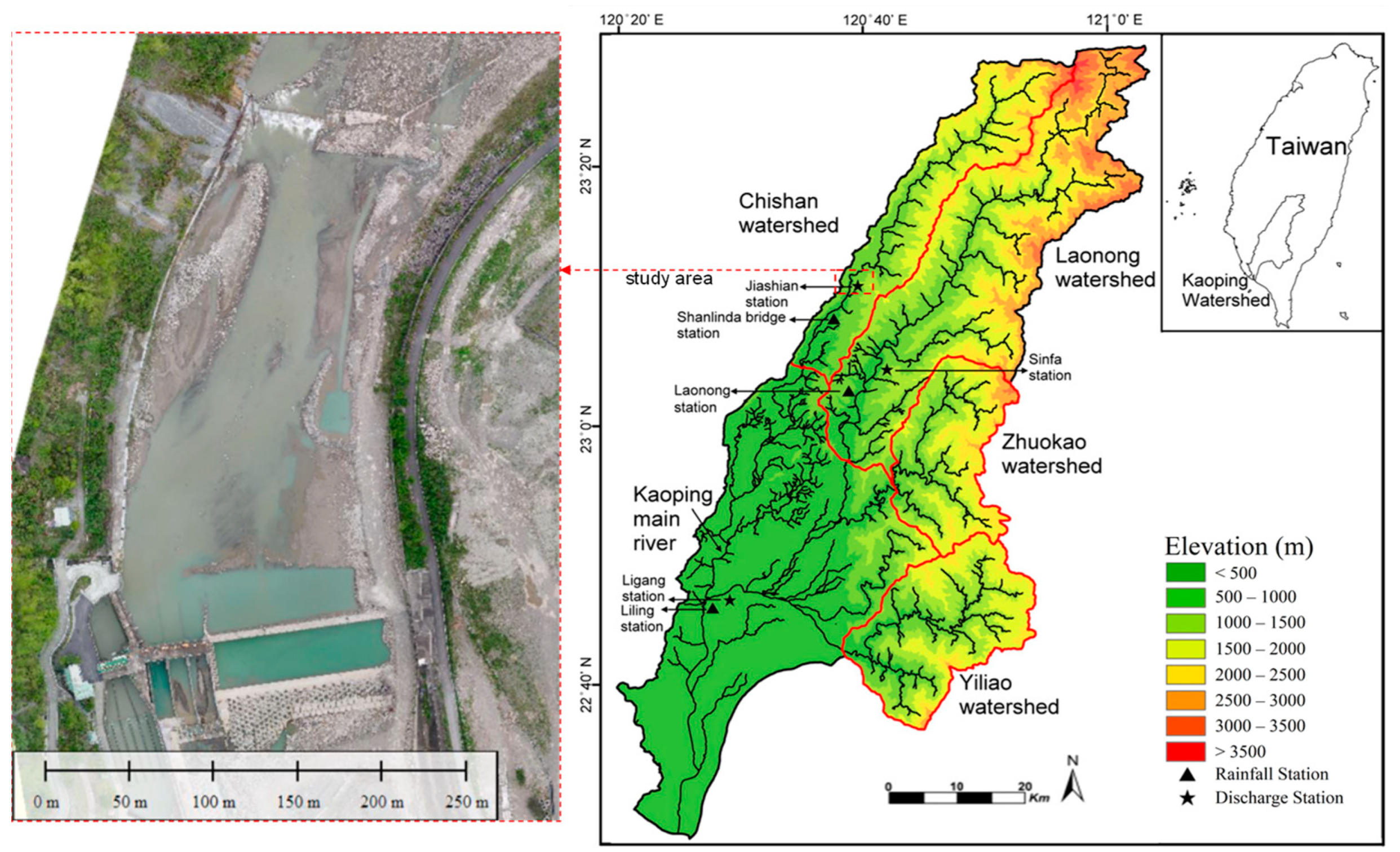
2.1. Study Area
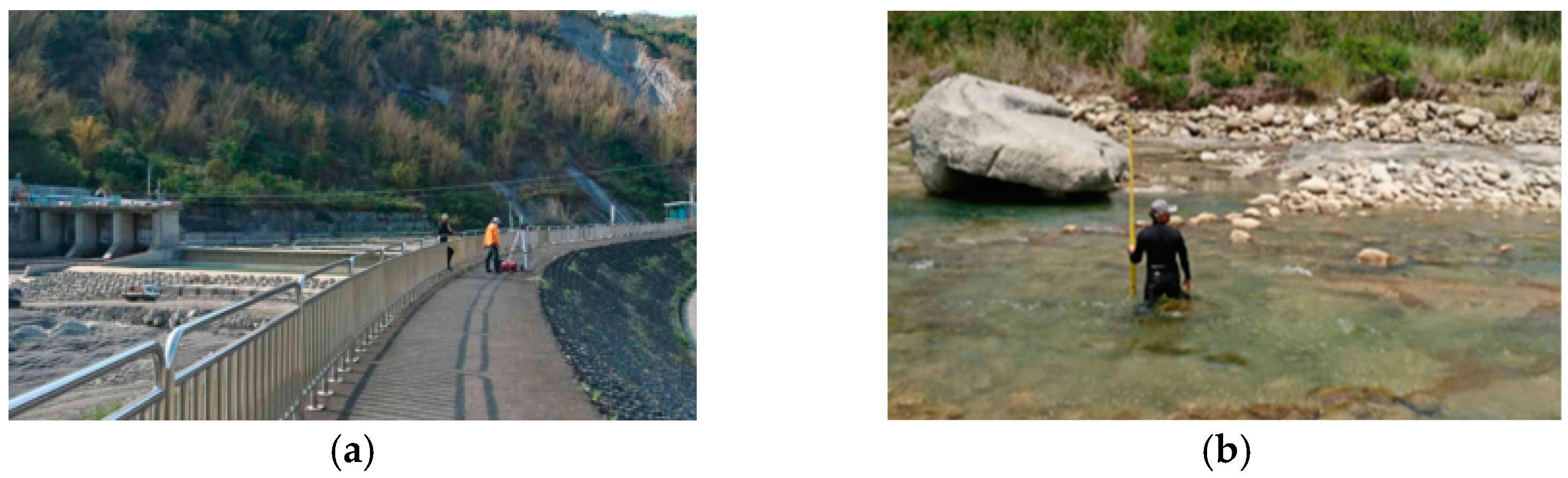
2.2. Bathymetry Investigation
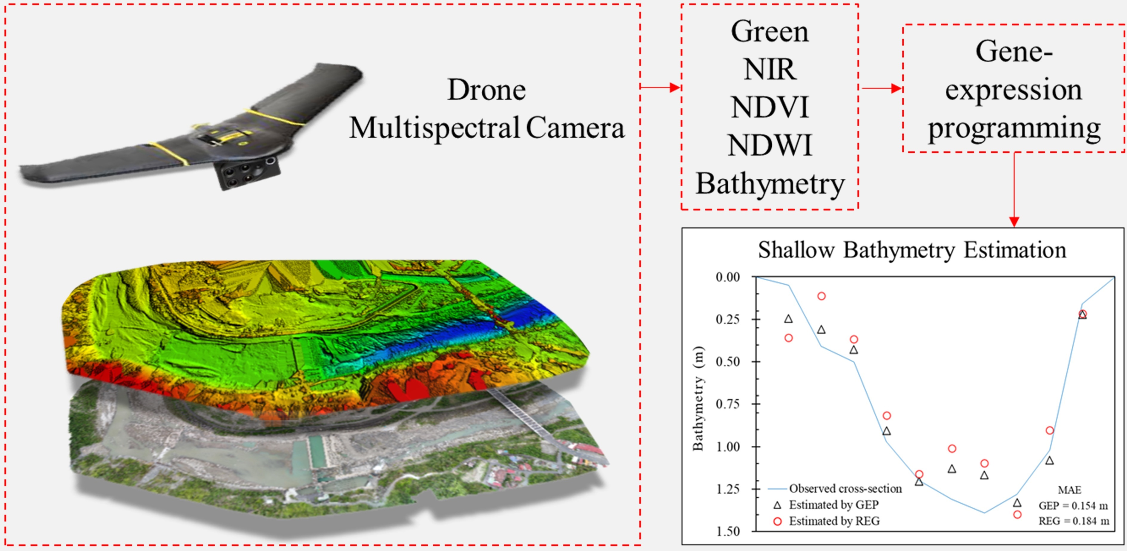
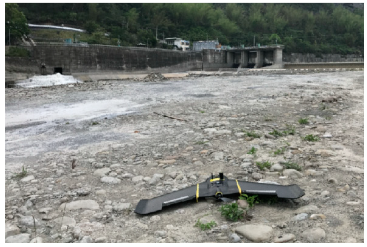
2.3. UAV and Multispectral Camera
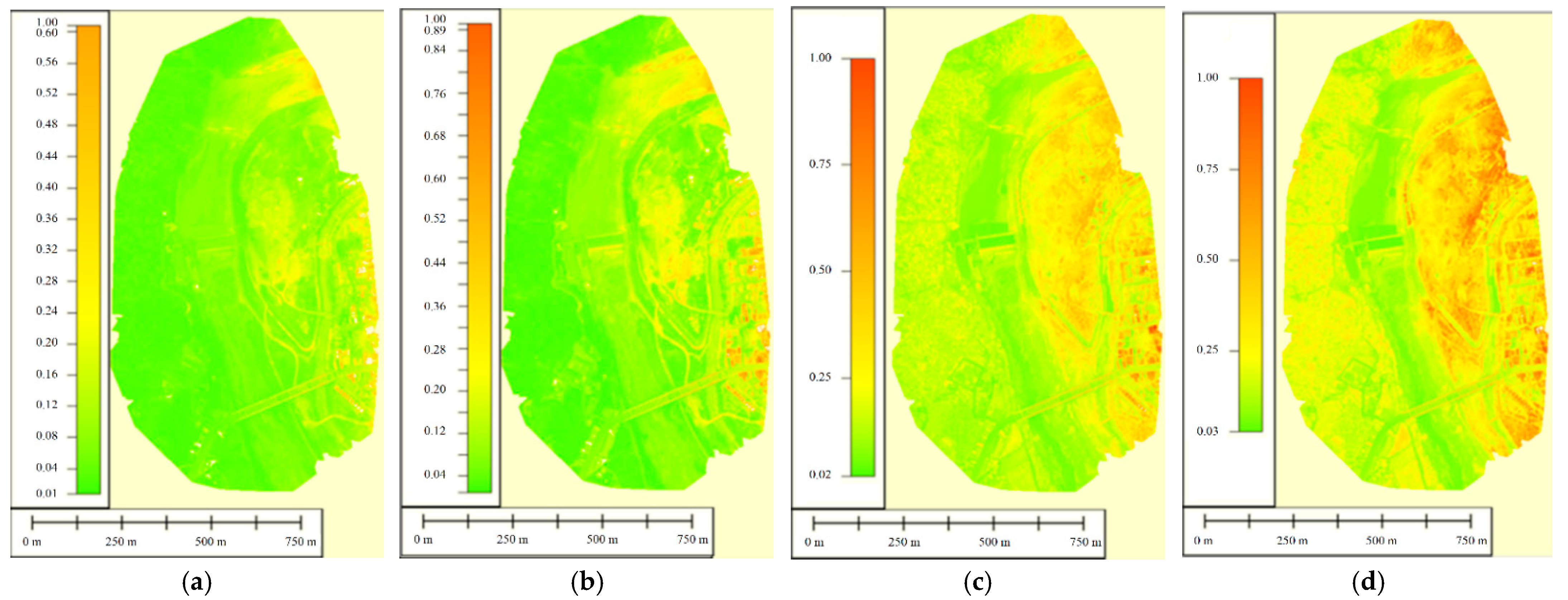
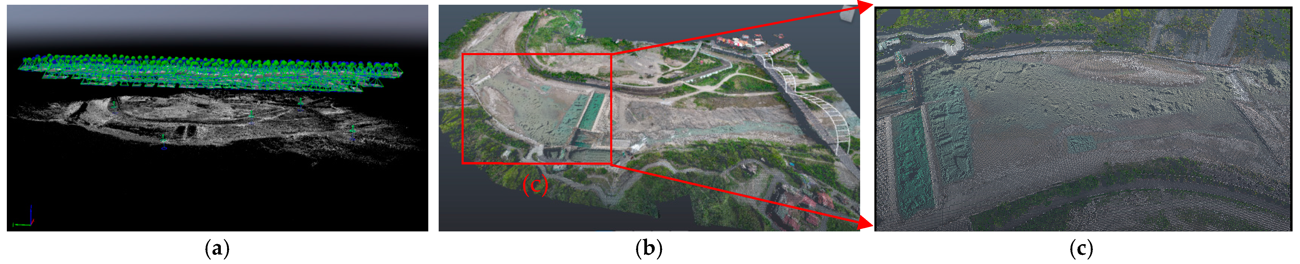
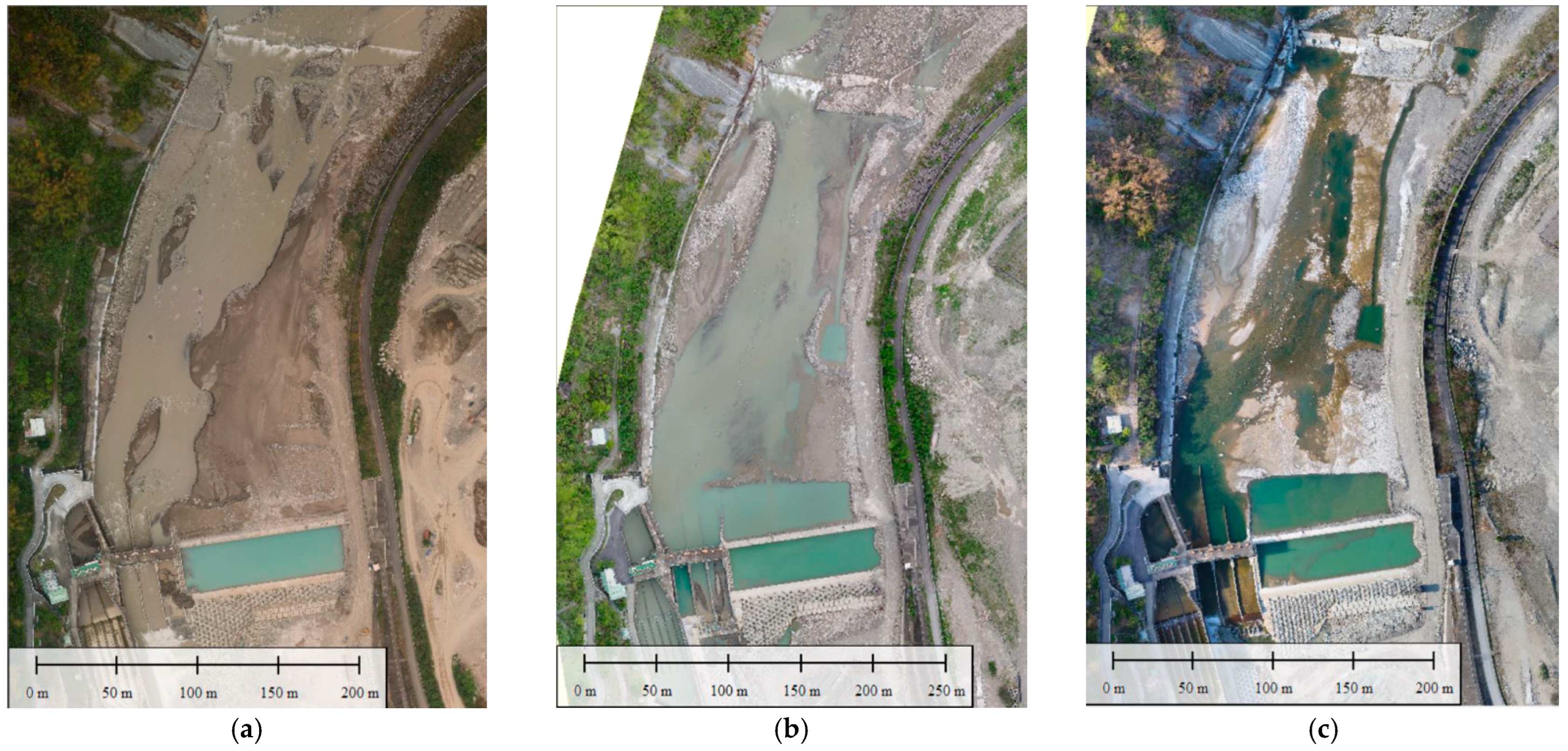
2.4. Data Processing
2.5. Development of Water Depth Retrieval Model
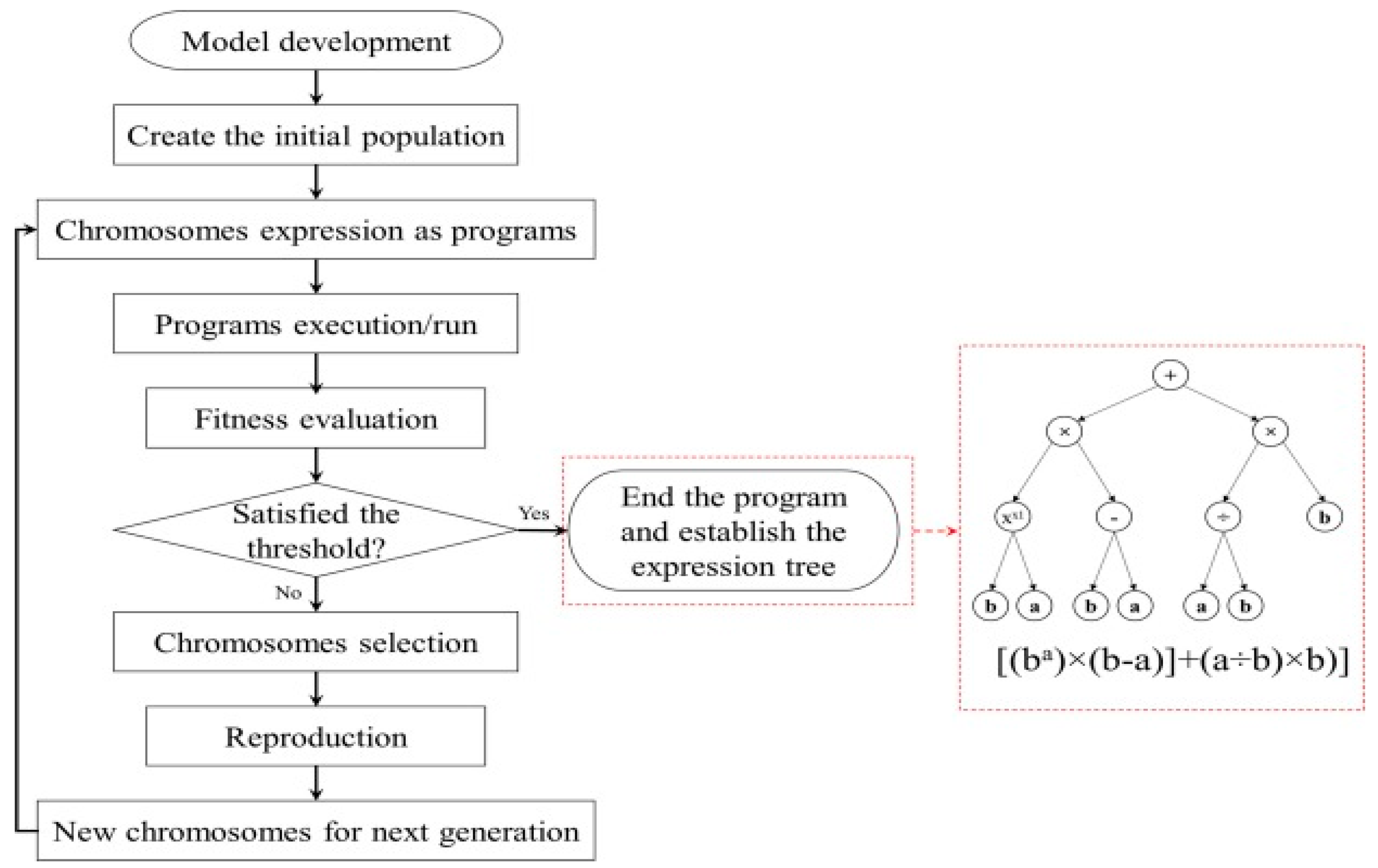
2.5.1. Gene-Expression Programming (GEP)
2.5.2. Simple Linear Regression (REG)
2.6. Model Accuracy Evaluation
3. Results
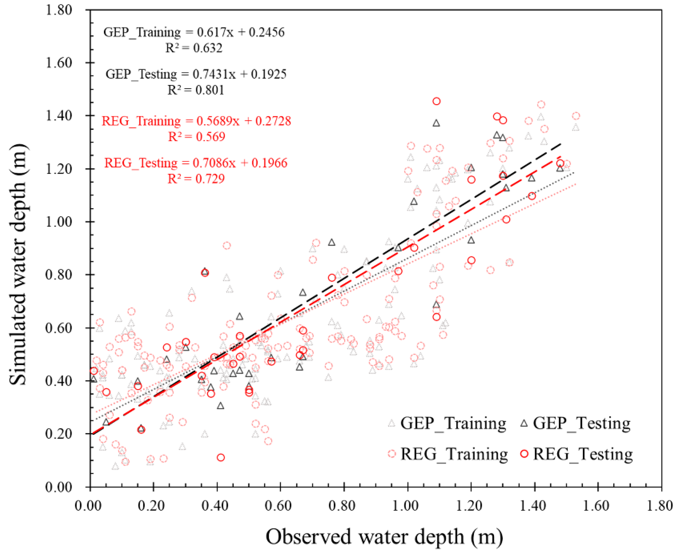
3.1. Simulation Results and Accuracy Evaluation
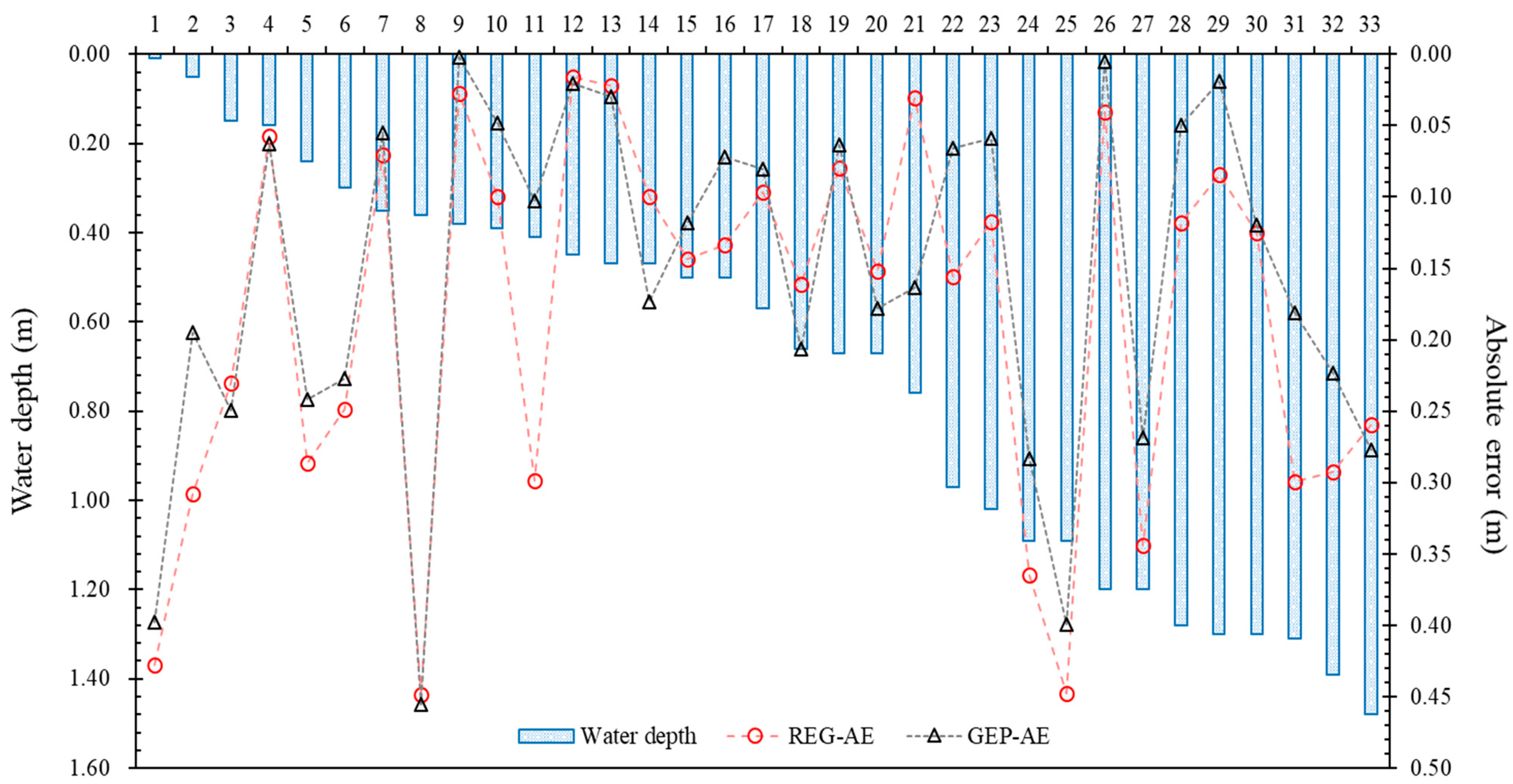
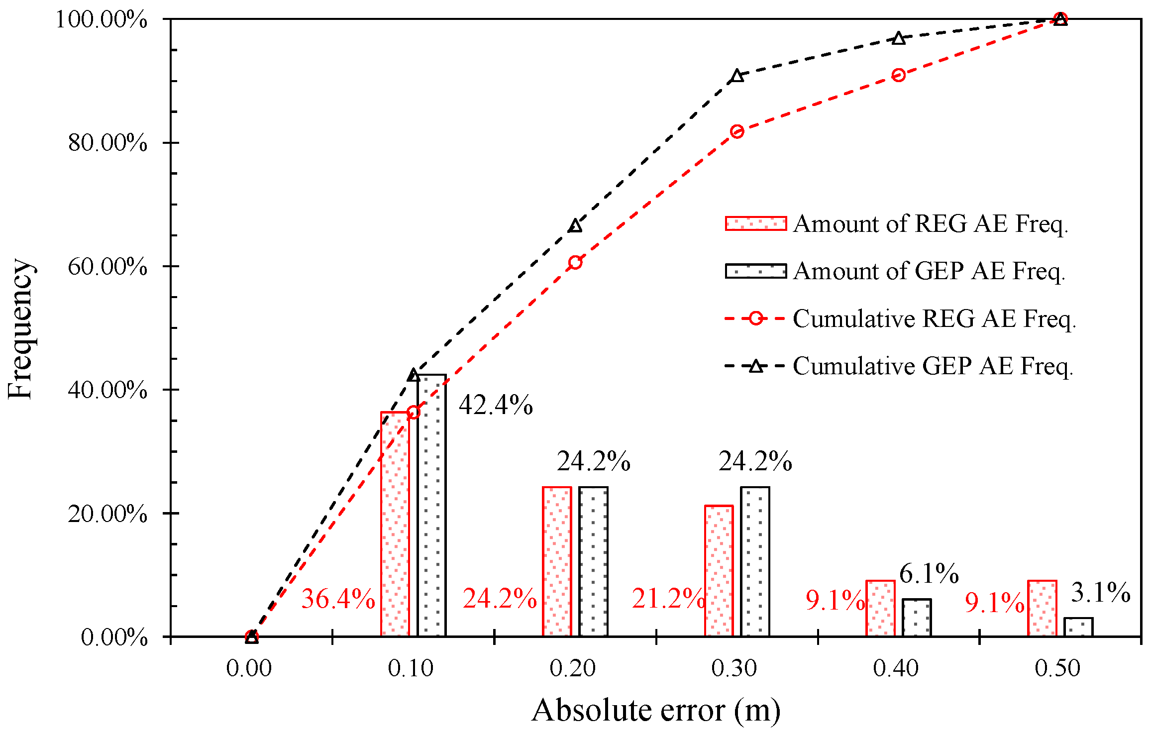
3.2. Error Evaluation
4. Discussion
5. Conclusions
Author Contributions
Funding
Data Availability Statement
Conflicts of Interest
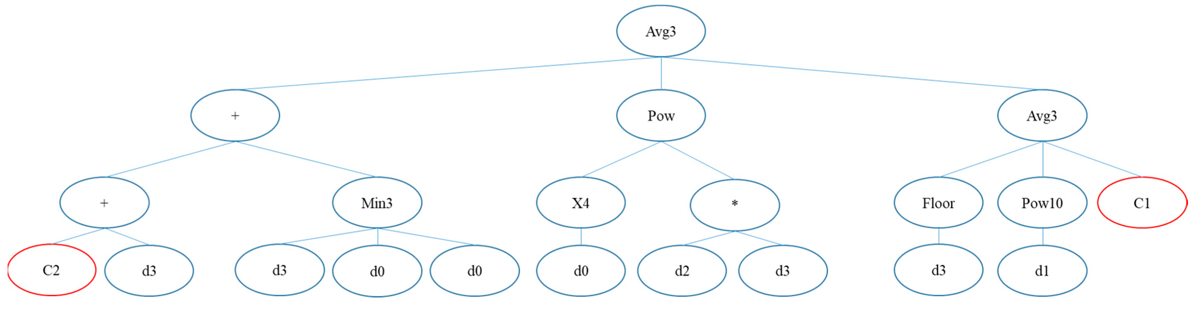
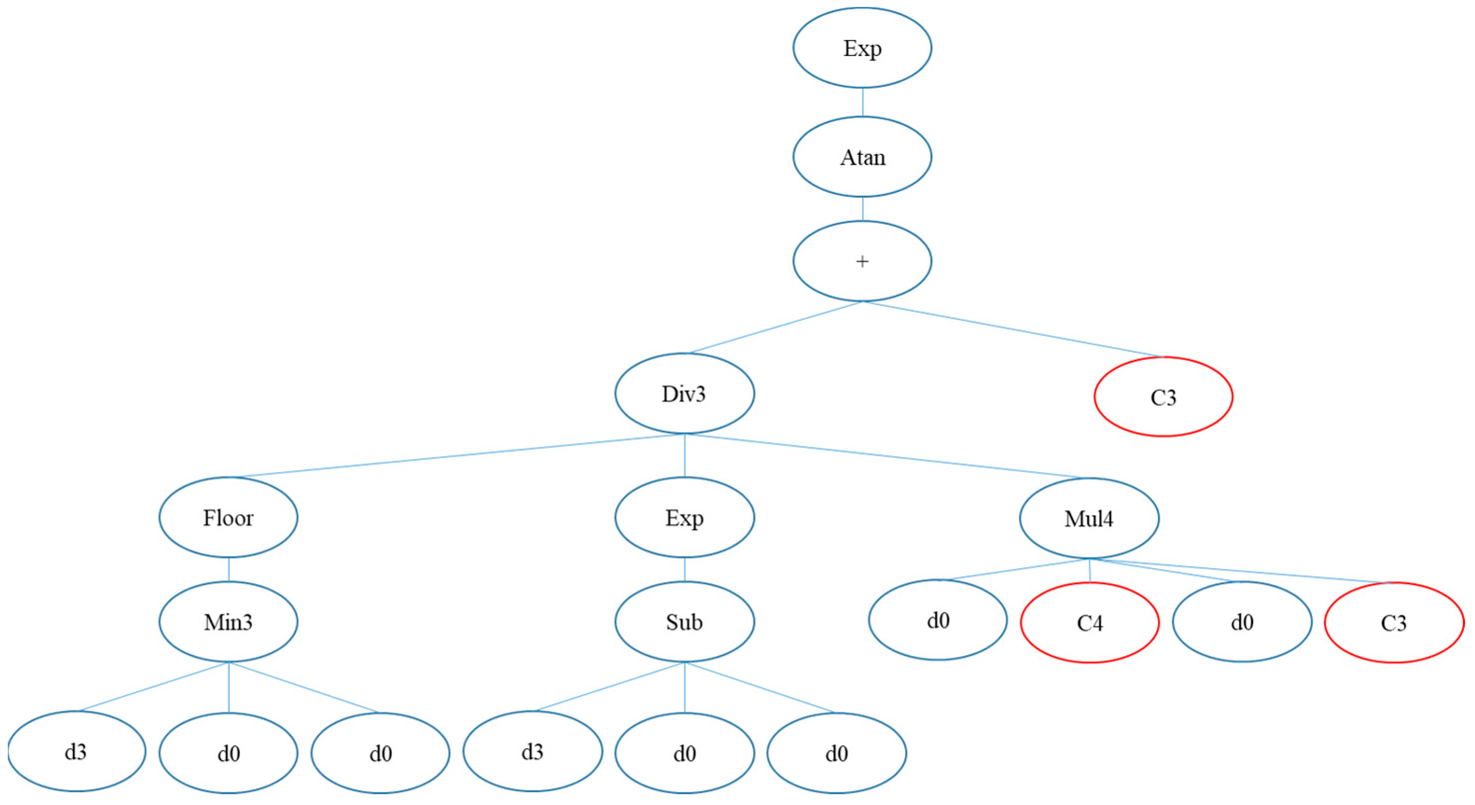
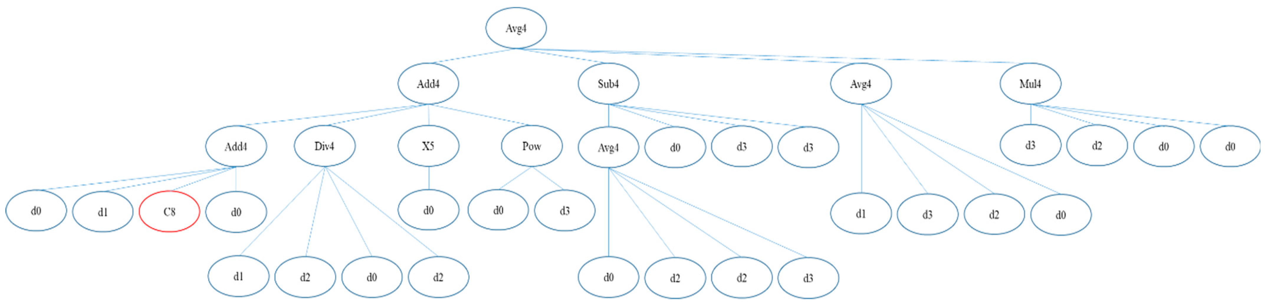
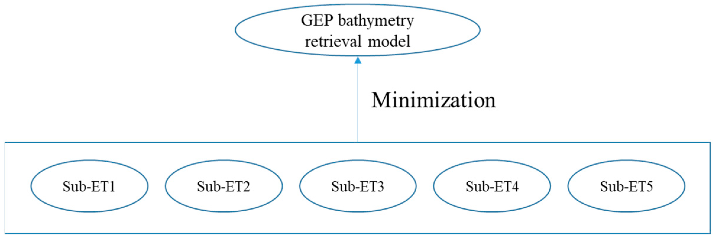
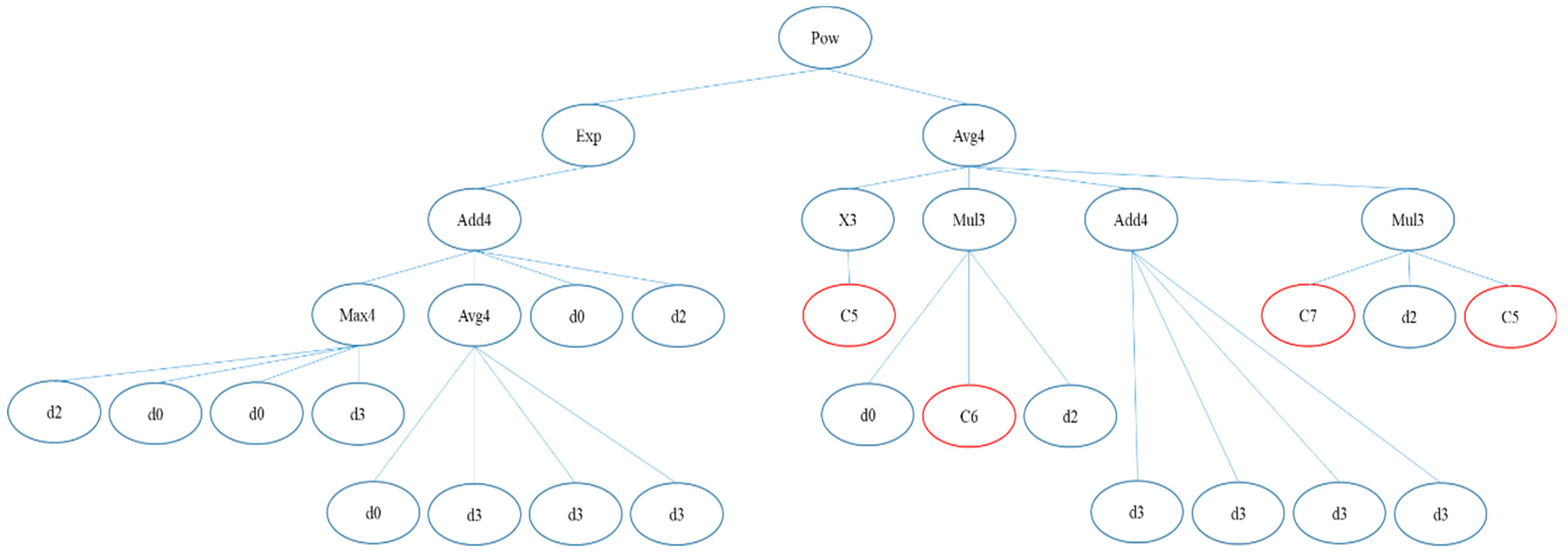
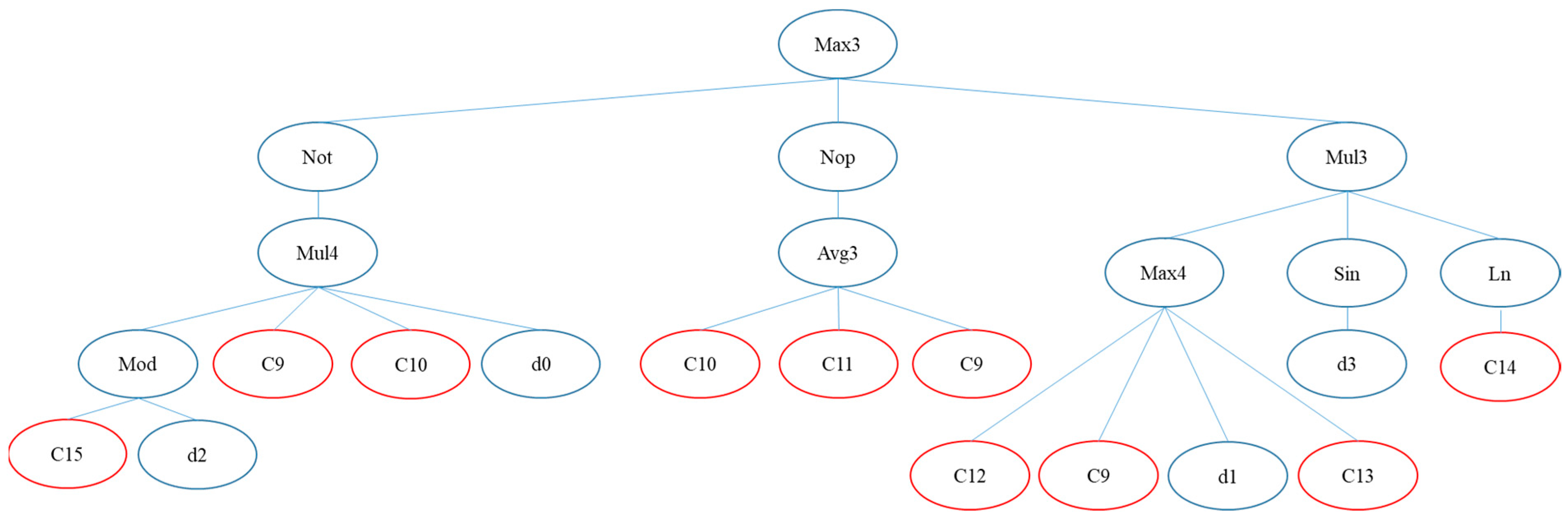
Appendix A. Sub-ETs of GEP Bathymetry Retrieval Model


Appendix B. Python-Based Code for Shallow Water Depth Retrieval by UAV Imagery
- y = ((((C2+d[3])*min(d[3],d[0],d[0]))+pow(pow(d[0],4.0),(d[2]*d[3]))+((floor (d[3])+pow(10.0,d[1])+C1)/3.0))/3.0)
- y = min(y,exp(atan(((floor(min(d[0],d[2],d[0]))/exp((d[0]-d[2]-d[3]))/(d[0]*C4* d[0]*C3))+C3))))
- y = min(y,pow(exp((max(d[2],d[0],d[0],d[3])+((d[0]+d[3]+d[3]+d[3])/4.0)+d[0]+ d[2])),((pow(C5,3.0)+(d[0]*C6*d[2])+(d[3]+d[3]+d[3]+d[3])+(C7*d[2]*C5))/4.0)))
- y = min(y,((((d[0]+d[1]+C8+d[0])+(d[1]/d[2]/d[0]/d[2])+pow(d[0],5.0)+pow (d[0],d[3]))+(((d[0]+d[2]+d[2]+d[3])/4.0)-d[0]-d[3]-d[3])+((d[1]+d[3]+d[2]+d[0]) /4.0)+(d[3]*d[2]*d[0]*d[0]))/4.0))
- y = min(y,max((1.0-(gepMod(C15,d[2])*C9*C10*d[0])),(((C10+C11+C12)/3.0)), (max(C12,C9,d[1],C13)*sin(d[3])*log(C14))))
References
- G.R.W.M. Committee. The 2018 Annual Report on the Management and Implementation of Kaoping River Basin. 2019. [Google Scholar]
- Dadson, S.J.; Hovius, N.; Chen, H.; Dade, W.B.; Hsieh, M.-L.; Willett, S.D.; Hu, J.-C.; Horng, M.-J.; Chen, M.-C.; Stark, C.P.; et al. Links between erosion, runoff variability and seismicity in the Taiwan orogen. Nature 2003, 426, 648–651. [Google Scholar] [CrossRef] [PubMed]
- Dierssen, H.M.; Theberge, A.E. Bathymetry: Seafloor mapping history. In Coastal and Marine Environments; CRC Press: Boca Raton, FL, USA, 2020; pp. 195–202. [Google Scholar]
- Gustafsson, H.; Zuna, L. Unmanned Aerial Vehicles for Geographic Data Capture: A Review. Bachelor’s Thesis, School of Architecture and the Built Environment, Kensington, NSW, Australia, 2017. [Google Scholar]
- Heblinski, J.; Schmieder, K.; Heege, T.; Agyemang, T.K.; Sayadyan, H.; Vardanyan, L. High-resolution satellite remote sensing of littoral vegetation of Lake Sevan (Armenia) as a basis for monitoring and assessment. Hydrobiologia 2011, 661, 97–111. [Google Scholar] [CrossRef]
- Huang, M.Y.F.; Montgomery, D.R. Fluvial response to rapid episodic erosion by earthquake and typhoons, Tachia River, central Taiwan. Geomorphology 2012, 175–176, 126–138. [Google Scholar] [CrossRef]
- Kasvi, E.; Laamanen, L.; Lotsari, E.; Alho, P. Flow Patterns and Morphological Changes in a Sandy Meander Bend during a Flood—Spatially and Temporally Intensive ADCP Measurement Approach. Water 2017, 9, 106. [Google Scholar] [CrossRef] [Green Version]
- Munawar, H.S.; Ullah, F.; Qayyum, S.; Heravi, A. Application of Deep Learning on UAV-Based Aerial Images for Flood Detection. Smart Cities 2021, 4, 65. [Google Scholar] [CrossRef]
- Samboko, H.T.; Abas, I.; Luxemburg, W.M.J.; Savenije, H.H.G.; Makurira, H.; Banda, K.; Winsemius, H.C. Evaluation and improvement of remote sensing-based methods for river flow management. Phys. Chem. Earth Parts A/B/C 2020, 117, 102839. [Google Scholar] [CrossRef]
- Tamminga, A.; Hugenholtz, C.; Eaton, B.; Lapointe, M. Hyperspatial Remote Sensing of Channel Reach Morphology and Hydraulic Fish Habitat Using an Unmanned Aerial Vehicle (UAV): A First Assessment in the Context of River Research and Management. River Res. Appl. 2015, 31, 379–391. [Google Scholar] [CrossRef]
- Kostaschuk, R.A.; Church, M.A. Macroturbulence generated by dunes: Fraser River, Canada. Sediment. Geol. 1993, 85, 25–37. [Google Scholar] [CrossRef]
- Alevizos, E.; Alexakis, D.D. Evaluation of radiometric calibration of drone-based imagery for improving shallow bathymetry retrieval. Remote Sens. Lett. 2022, 13, 311–321. [Google Scholar] [CrossRef]
- Kammerer, E.; Charlot, D.; Guillaudeux, S.; Michaux, P. Comparative study of shallow water multibeam imagery for cleaning bathymetry sounding errors. In Proceedings of the MTS/IEEE Oceans 2001. An Ocean Odyssey. Conference Proceedings (IEEE Cat. No. 01CH37295), Honolulu, HI, USA, 5–8 November 2001; Volume 2124, pp. 2124–2128. [Google Scholar]
- Pacheco, A.; Horta, J.; Loureiro, C.; Ferreira, Ó. Retrieval of nearshore bathymetry from Landsat 8 images: A tool for coastal monitoring in shallow waters. Remote Sens. Environ. 2015, 159, 102–116. [Google Scholar] [CrossRef] [Green Version]
- Hernandez, W.J.; Armstrong, R.A. Deriving Bathymetry from Multispectral Remote Sensing Data. J. Mar. Sci. Eng. 2016, 4, 8. [Google Scholar] [CrossRef]
- Kasvi, E.; Salmela, J.; Lotsari, E.; Kumpula, T.; Lane, S.N. Comparison of remote sensing based approaches for mapping bathymetry of shallow, clear water rivers. Geomorphology 2019, 333, 180–197. [Google Scholar] [CrossRef]
- Kim, J.S.; Baek, D.; Seo, I.W.; Shin, J. Retrieving shallow stream bathymetry from UAV-assisted RGB imagery using a geospatial regression method. Geomorphology 2019, 341, 102–114. [Google Scholar] [CrossRef]
- Janowski, L.; Wroblewski, R.; Rucinska, M.; Kubowicz-Grajewska, A.; Tysiac, P. Automatic classification and mapping of the seabed using airborne LiDAR bathymetry. Eng. Geol. 2022, 301, 106615. [Google Scholar] [CrossRef]
- Ashphaq, M.; Srivastava, P.K.; Mitra, D. Review of near-shore satellite derived bathymetry: Classification and account of five decades of coastal bathymetry research. J. Ocean. Eng. Sci. 2021, 6, 340–359. [Google Scholar] [CrossRef]
- Bures, L.; Sychova, P.; Maca, P.; Roub, R.; Marval, S. River Bathymetry Model Based on Floodplain Topography. Water 2019, 11, 1287. [Google Scholar] [CrossRef] [Green Version]
- Jérôme, L.; Gentile, V.; Demarchi, L.; Spitoni, M.; Piégay, H.; Mróz, M. Bathymetric Mapping of Shallow Rivers with UAV Hyperspectral Data. In Proceedings of the Fifth International Conference on Telecommunications and Remote Sensing, Milan, Italy, 10–11 October 2016; pp. 43–49. [Google Scholar]
- Van-An, N.; Hsuan, R.; Chih-Yuan, H.; Kuo-Hsin, T. Bathymetry derivation in shallow water of the South China Sea with ICESat-2 and Sentinel-2 data. J. Appl. Remote Sens. 2021, 15, 044513. [Google Scholar] [CrossRef]
- Lee, C.B.; Traganos, D.; Reinartz, P. A Simple Cloud-Native Spectral Transformation Method to Disentangle Optically Shallow and Deep Waters in Sentinel-2 Images. Remote Sens. 2022, 14, 590. [Google Scholar] [CrossRef]
- Wu, C.-H.; Chen, S.-C.; Chou, H.-T. Geomorphologic characteristics of catastrophic landslides during typhoon Morakot in the Kaoping Watershed, Taiwan. Eng. Geol. 2011, 123, 13–21. [Google Scholar] [CrossRef]
- Wang, Y.-M.; Traore, S.; Kerh, T. Using artificial neural networks for modeling suspended sediment concentration. In Proceedings of the 10th WSEAS International Conference on Mathematical Methods and Computational Techniques in Electrical Engineering, Sofia, Bulgaria, 2–4 May 2008. [Google Scholar]
- Water Resources Bureau of Southern District, Water Resources Agency, Ministry of Economic Affairs. Research and Analysis Project for Water Quality Variation Factors and Water Diversion Timing of Jiaxian Weir; Water Resources Bureau of Southern District, Water Resources Agency, Ministry of Economic Affairs: Taipei City, Taiwan, 2003.
- Water Resources Administration, Ministry of Economic Affairs. Analysis of Rainfall and Flood Flow of Typhoon Morakot; Water Resources Administration, Ministry of Economic Affairs: Taipei City, Taiwan, 2009.
- Carlson, T.N.; Ripley, D.A. On the relation between NDVI, fractional vegetation cover, and leaf area index. Remote Sens. Environ. 1997, 62, 241–252. [Google Scholar] [CrossRef]
- McFeeters, S.K. The use of the Normalized Difference Water Index (NDWI) in the delineation of open water features. Int. J. Remote Sens. 1996, 17, 1425–1432. [Google Scholar] [CrossRef]
- Ma, S.; Tao, Z.; Yang, X.; Yu, Y.; Zhou, X.; Li, Z. Bathymetry Retrieval From Hyperspectral Remote Sensing Data in Optical-Shallow Water. IEEE Trans. Geosci. Remote Sens. 2014, 52, 1205–1212. [Google Scholar] [CrossRef]
- Misra, A.; Ramakrishnan, B. Assessment of coastal geomorphological changes using multi-temporal Satellite-Derived Bathymetry. Cont. Shelf Res. 2020, 207, 104213. [Google Scholar] [CrossRef]
- Liu, L.-W.; Ma, X.; Wang, Y.-M.; Lu, C.-T.; Lin, W.-S. Using artificial intelligence algorithms to predict rice (Oryza sativa L.) growth rate for precision agriculture. Comput. Electron. Agric. 2021, 187, 106286. [Google Scholar] [CrossRef]
- Liu, L.-W.; Wang, Y.-M. Modelling Reservoir Turbidity Using Landsat 8 Satellite Imagery by Gene Expression Programming. Water 2019, 11, 1479. [Google Scholar] [CrossRef] [Green Version]
- Su, H.; Liu, H.; Heyman, W.D. Automated Derivation of Bathymetric Information from Multi-Spectral Satellite Imagery Using a Non-Linear Inversion Model. Mar. Geod. 2008, 31, 281–298. [Google Scholar] [CrossRef]
- Ferreira, C. Gene Expression Programming in Problem Solving. In Soft Computing and Industry: Recent Applications; Roy, R., Köppen, M., Ovaska, S., Furuhashi, T., Hoffmann, F., Eds.; Springer: London, UK, 2002; pp. 635–653. [Google Scholar]
- Liu, L.-W.; Lu, C.-T.; Wang, Y.-M.; Lin, K.-H.; Ma, X.; Lin, W.-S. Rice (Oryza sativa L.) Growth Modeling Based on Growth Degree Day (GDD) and Artificial Intelligence Algorithms. Agriculture 2022, 12, 59. [Google Scholar] [CrossRef]
- Wang, X.; Liu, L.; Zhang, W.; Ma, X. Prediction of Plant Uptake and Translocation of Engineered Metallic Nanoparticles by Machine Learning. Environ. Sci. Technol. 2021, 55, 7491–7500. [Google Scholar] [CrossRef]
- Ressel, R.; Singha, S.; Lehner, S.; Rösel, A.; Spreen, G. Investigation into Different Polarimetric Features for Sea Ice Classification Using X-Band Synthetic Aperture Radar. IEEE J. Sel. Top. Appl. Earth Obs. Remote Sens. 2016, 9, 3131–3143. [Google Scholar] [CrossRef] [Green Version]
- Mandlburger, G.; Kölle, M.; Nübel, H.; Soergel, U. BathyNet: A Deep Neural Network for Water Depth Mapping from Multispectral Aerial Images. PFG-J. Photogramm. Remote Sens. Geoinf. Sci. 2021, 89, 71–89. [Google Scholar] [CrossRef]
- Sagawa, T.; Yamashita, Y.; Okumura, T.; Yamanokuchi, T. Satellite Derived Bathymetry Using Machine Learning and Multi-Temporal Satellite Images. Remote Sens. 2019, 11, 1155. [Google Scholar] [CrossRef] [Green Version]
- Sandidge, J.C.; Holyer, R.J. Coastal Bathymetry from Hyperspectral Observations of Water Radiance. Remote Sens. Environ. 1998, 65, 341–352. [Google Scholar] [CrossRef]


| Items | 6 April 2016 | 10 April 2017 | 2 May 2017 |
|---|---|---|---|
| Images | 772 | 1076 | 856 |
| Median of Key-points per Image | 20,000 | 21,111 | 53,203 |
| Median of Matching Points per Image | 8870.85 | 5889.67 | 12,485.60 |
| Ground Control Points (GCP) | 20 | 19 | 6 |
| The Mean RMS Error of GCP in X-axis | 0.009 m | 0.006 m | 0.003 m |
| The Mean RMS Error of GCP in Y-axis | 0.007 m | 0.004 m | 0.004 m |
| The Mean RMS Error of GCP in Z-axis | 0.013 m | 0.008 m | 0.004 m |
| Number of 3D Densified Points | 97,694,554 | 125,818,685 | 400,257,260 |
| Average Density (per m3) | 37.37 | 64.61 | 776.11 |
| Index | Max | Min | Average | Standard Deviation |
|---|---|---|---|---|
| Green | 0.094 | 0.038 | 0.071 | 0.008 |
| NIR | 0.079 | 0.044 | 0.065 | 0.008 |
| NDVI | 0.148 | −0.323 | −0.163 | 0.071 |
| NDWI | 0.264 | −0.290 | 0.044 | 0.093 |
| Variable | Average Values of Variables | p-Value | Significant Difference | ||
|---|---|---|---|---|---|
| Raw Dataset | Training | Testing | |||
| Green | 0.071 | 0.070 | 0.072 | 0.411 | - |
| NIR | 0.065 | 0.065 | 0.064 | 0.446 | - |
| NDVI | −0.163 | −0.162 | −0.172 | 0.450 | - |
| NDWI | 0.044 | 0.041 | 0.063 | 0.244 | - |
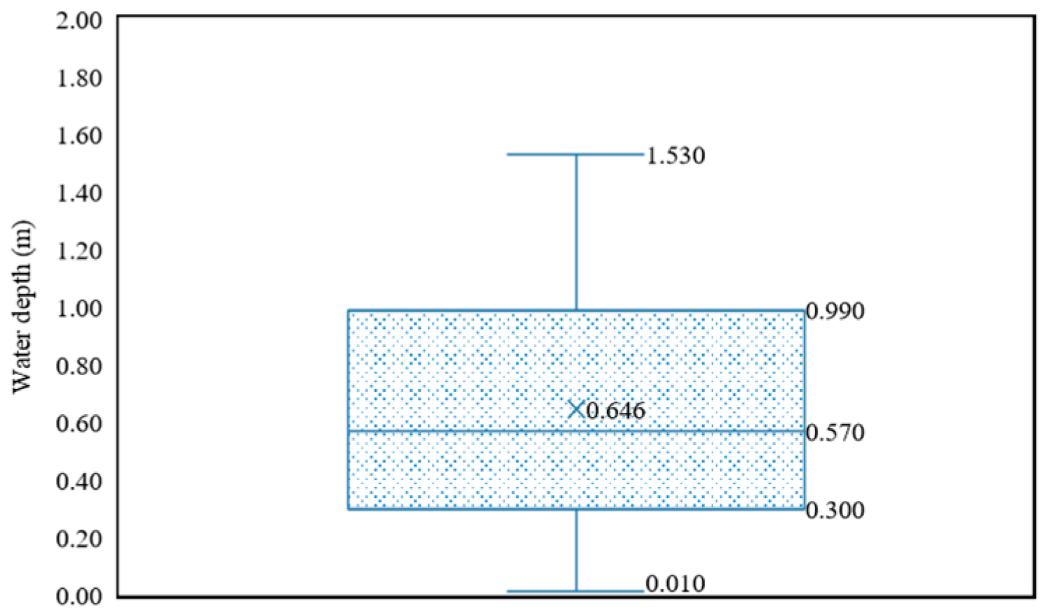
| Water Depth (m) | 0.646 | 0.633 | 0.701 | 0.386 | - |
| Model | R2 | MAE (m) | ME (m) | RMSE (m) | ||||
|---|---|---|---|---|---|---|---|---|
| Training | Testing | Training | Testing | Training | Testing | Training | Testing | |
| GEP | 0.632 | 0.801 | 0.188 | 0.154 | 0.003 | 0.012 | 0.242 | 0.195 |
| REG | 0.569 | 0.729 | 0.211 | 0.184 | <0.001 | −0.008 | 0.262 | 0.225 |
| Model | Observed Bathymetry (m) | |||
|---|---|---|---|---|
| <0.4 | 0.4–0.8 | 0.8–1.48 | 0–1.48 | |
| MAE (m) | ||||
| GEP | 0.194 | 0.110 | 0.163 | 0.154 |
| REG | 0.220 | 0.112 | 0.221 | 0.184 |
| Study | Tool | Factor | Value (m) | Range (m) | |
|---|---|---|---|---|---|
| Method | Remote/Contact 1 | ||||
| Kasvi et al. [16] | ADCP 2 | C | MAE | 0.030–0.070 (avg. 0.053) | 0.20–1.50 |
| Kasvi et al. [16] | REG | R | MAE | 0.050–0.170 (avg. 0.112) | 0.00–1.50 |
| This study | ML (GEP) | R | MAE | 0.154 | 0.01–1.53 |
| This study | REG | R | MAE | 0.184 | 0.01–1.53 |
| Kasvi et al. [16] | SfM | R | MAE | 0.180–2.980 (avg. 0.740) | 0.00–1.50 |
| This study | REG | R | ME | −0.008 | 0.01–1.53 |
| This study | ML (GEP) | R | ME | 0.012 | 0.01–1.53 |
| Kasvi et al. [16] | ADCP 2 | C | ME | −0.030–0.000 (avg. −0.015) | 0.20–1.50 |
| Kasvi et al. [16] | REG | R | ME | −0.170–0.020 (avg. −0.087) | 0.00–1.50 |
| Jérôme et al. [21] | REG | R | ME | 0.130 | 0.09–1.01 |
| Mandlburger et al. [39] | ML (DL) | R | ME | 0.150 | 0.00–12.00 |
| Kasvi et al. [16] | SfM | R | ME | −0.180–3.200 (avg. 0.357) | 0.00–1.50 |
| Sagawa et al. [40] | ML (RF) | R | ME | 0.250–1.370 (avg. 1.008) | 0.00–5.00 |
| This study | ML (GEP) | R | RMSE | 0.195 | 0.01–1.53 |
| This study | REG | R | RMSE | 0.225 | 0.01–1.53 |
| Lee et al. [23] | ML (NN) | R | RMSE | 0.310–0.400 (avg. 0.358) | 1.50–9.00 |
| Lee et al. [23] | MBVA | R | RMSE | 0.440 | 1.50–9.00 |
| Sandidge and Holyer [41] | ML (NN) | R | RMSE | 0.480 | 0.00–6.00 |
| Lee et al. [23] | ML (NN) | R | RMSE | 0.510–0.520 (avg. 0.515) | 1.00–11.00 |
| Lee et al. [23] | MBVA | R | RMSE | 0.540 | 1.00–11.00 |
| Lee et al. [23] | TBRA | R | RMSE | 1.020 | 1.50–9.00 |
| Lee et al. [23] | TBRA | R | RMSE | 1.250 | 1.00–11.00 |
| Hernandez and Armstrong [15] | REG | R | RMSE | 1.260 | 1.00–10.00 |
| Su et al. [34] | REG | R | RMSE | 1.340 | 0.00–5.00 |
| Sagawa et al. [40] | ML (RF) | R | RMSE | 0.830–1.910 (avg. 1.634) | 0.00–5.00 |
| Su et al. [34] | ML (LM) | R | RMSE | 2.070 | 0.00–5.00 |
Publisher’s Note: MDPI stays neutral with regard to jurisdictional claims in published maps and institutional affiliations. |
© 2022 by the authors. Licensee MDPI, Basel, Switzerland. This article is an open access article distributed under the terms and conditions of the Creative Commons Attribution (CC BY) license (https://creativecommons.org/licenses/by/4.0/).
Share and Cite
Lee, C.-H.; Liu, L.-W.; Wang, Y.-M.; Leu, J.-M.; Chen, C.-L. Drone-Based Bathymetry Modeling for Mountainous Shallow Rivers in Taiwan Using Machine Learning. Remote Sens. 2022, 14, 3343. https://doi.org/10.3390/rs14143343
Lee C-H, Liu L-W, Wang Y-M, Leu J-M, Chen C-L. Drone-Based Bathymetry Modeling for Mountainous Shallow Rivers in Taiwan Using Machine Learning. Remote Sensing. 2022; 14(14):3343. https://doi.org/10.3390/rs14143343
Chicago/Turabian StyleLee, Chih-Hung, Li-Wei Liu, Yu-Min Wang, Jan-Mou Leu, and Chung-Ling Chen. 2022. "Drone-Based Bathymetry Modeling for Mountainous Shallow Rivers in Taiwan Using Machine Learning" Remote Sensing 14, no. 14: 3343. https://doi.org/10.3390/rs14143343
APA StyleLee, C.-H., Liu, L.-W., Wang, Y.-M., Leu, J.-M., & Chen, C.-L. (2022). Drone-Based Bathymetry Modeling for Mountainous Shallow Rivers in Taiwan Using Machine Learning. Remote Sensing, 14(14), 3343. https://doi.org/10.3390/rs14143343