Assessing the Spatiotemporal Variability of SMAP Soil Moisture Accuracy in a Deciduous Forest Region

Abstract

The goal of this study is to assess the temporal variability of the performance of the Soil Moisture Active Passive, SMAP, soil moisture retrievals throughout the seasons as surface conditions change. In-situ soil moisture observations from a network deployed in Millbrook, New York, between 2019 and 2021 are used. The network comprises 25 stations distributed across a 33-km SMAP pixel with a predominantly forest land cover. The in-situ soil moisture observations were collected between 6 and 7 a.m., local time. This article covers the assessment of the temporal accuracy of SMAP soil moisture by incorporating various upscaling methods. Four upscaling methods are used in this study: arithmetic average, Voronoi diagram, topographic wetness index, and land cover weighted average. The agreement between SMAP soil moisture and the upscaled in-situ measurements was gauged using the root-mean-squared difference, the mean difference, and the unbiased root-mean-squared difference. The consistency of the temporal variability of SMAP soil moisture data resulting from the four upscaling methods was analyzed. The results revealed that SMAP retrievals (soil moisture data) are systematically higher than in situ observations during the different seasons. The results indicate that the highest performance of SMAP soil moisture retrievals is in September with an ubRMSD value of 0.03 m³.m⁻³ for the morning and evening overpasses, which can be attributed to a lower vegetation density during the seasonal transition. The agreement with in-situ observations degrades during March–April with ubRMSD values above 0.04 m³.m⁻³, reaching ~0.06 m³.m⁻³ in April, which can be attributed to the non-reliability of in-situ measurements due to freeze\thaw transition and the challenging determination of the soil effective temperature. The ubRMSD is also higher than 0.04 m³.m⁻³ in the months of May–June, which could be due to the introduced vegetation effect during the growth season. These findings are consistent across all the upscaling methods. The average ubRMSD over the study period is 0.055 m³.m⁻³, which falls short of meeting the mission’s performance target. This study proves the need to enhance SMAP retrieval over forest sites.

1. Introduction

Soil moisture plays a crucial role in the water and energy fluxes exchange between the different climate components [1,2]. It is vital to understand soil moisture spatio-temporal variability for several scientific studies and operational applications, including hydrological and meteorological modeling and agricultural applications [3]. For instance, understanding the patterns of soil moisture variability is useful for a variety of applications, including weather services and climate monitoring [4], agricultural production [5], soil conservation [6], and landscape management [7]. Thus, soil moisture plays a crucial role in many hydrological, biological, and ecological processes. Further, soil moisture influences the interactions between the land surface and the atmosphere, which in turn affects the climate and weather. Consequently, flood and drought forecasts, weather predictions, and crop growth models will be more accurate. In addition, decision-makers will have access to more effective tools. In-situ and remote sensing measurements, as well as land surface modeling, are the most common ways of obtaining soil moisture estimates. Soil moisture remote sensing at global and regional scales has evolved significantly in recent years. However, large uncertainties can be introduced in the retrieval of soil moisture due to the complexity of surface processes and measurement errors such as those resulting from the brightness temperature or radar backscatter [8,9]. It is, therefore, necessary to verify satellite-based soil moisture products using in situ measurements. The validation of satellite-based soil moisture observations throughout the seasons is vital to assess the accuracy and reliability of the product as surface conditions evolve and change seasonally [10]. The soil moisture retrieval can be influenced by several factors impacting the range of error, such as vegetation water content (VWC), vegetation-induced scattering, surface roughness, and temperature profile, which are all subjected to seasonal variabilities [11]. It is important to inform users on the evolve of the quality of soil moisture retrieval throughout the year. The mission requirements in terms of accuracy could be met on average over a long test period, but it is possible that the retrieved soil moisture overperforms and underperforms during specific months to maintain the overall average performance. It is important to depict the seasonal variability of the retrieval and identify the period during which the reliability of the product degrades so the users can proceed with caution.

Soil moisture remote sensing has been expanded since the launch of the SMAP mission on 31 January 2015. SMAP is an environmental research satellite, equipped with state-of-the-art instruments capable of mapping soil moisture and freeze/thaw state all over the globe [12]. SMAP provides valuable information for decision-makers and emergency managers by enabling the tracking of soil moisture and freeze/thaw variation over time. For this reason, several studies were carried out to validate SMAP soil moisture products [13,14,15,16,17,18].

The SMAP mission is tasked with achieving specific baseline standards for the accuracy of soil moisture retrieval. For land surfaces that are not covered with dense vegetation, frozen soil, snow cover, and complex topography, the targeted unbiased root-mean-square difference for SMAP retrievals is <0.04 m³.m⁻³ [3]. To ensure the quality and reliability of SMAP products, a rigorous validation process has been established. This process ensures conformity to mission requirements throughout the satellite’s operational lifetime. Therefore, information regarding the quality of the data can be communicated to users [19]. SMAP validation analyses have been updated annually and released in data product assessment reports, e.g., [14,15,20,21]. SMAP soil moisture products are generally evaluated using the Core Validation Sites (CVS), sparse network, and other satellite products [22]. CVS are an integral part of the SMAP calibration and validation process; they provide continuous soil moisture data measurements within a SMAP grid cell and provide confidence in the representativeness of a site [14]. In addition, the validation process is further reinforced by conducting field experiments in order to assess SMAP performance at sites with specific characteristics. In this context, the SMAP validation experiment 2016 (SMAPVEX16) evaluated the accuracy of SMAP retrievals in agricultural areas. Based on the findings of the study, the retrieval errors associated with SMAP were caused by the algorithm failing to adequately capture rapidly growing vegetation as well as early-season changes in surface conditions. Thus, field experiments can be helpful for investigating the source of SMAP soil moisture bias and for improving retrieval algorithms. The present study analyzes the performance of SMAP over forested areas at a 33-km spatial resolution.

The retrieval of soil moisture under heterogeneous land cover, forest, and high-latitude regions remains a challenge for the SMAP mission [17,19]. The SMAP mission has been in an extended phase since 2018. In the extended phase, one of the objectives is to validate soil moisture and vegetation optical depth retrievals in forested areas. Understanding the uncertainties that can be introduced in the retrieval of soil moisture in forested regions will contribute to the improvement of satellite-based soil moisture products in forested areas. Therefore, reliable information regarding the soil moisture status in a forested region contributes to a better understanding of the forested regions. This information assists in the development of research studies related to water supply, climate regulation, soil protection, and biodiversity conservation in forested ecosystems. Furthermore, forest resource managers rely on forest simulation models to estimate forest vegetation growth and dynamics [23]. The performance of such models can be enhanced by combining a reliable soil moisture dataset with wide spatial coverage.

A significant part of improving SMAP soil moisture retrievals can be addressed by conducting extensive field experiments, identifying the sources of the observed soil moisture biases, and improving the retrieval algorithms. SMAP products have been validated through upscaling of in situ observations with the assumption that in situ measurements have negligible errors compared to satellite estimates [24]. In situ observations are obtained from permanent networks or temporary measurements collected during field campaigns. To match satellite pixels with ground-based soil moisture measurements, several upscaling approaches were tested, and their results are reported in the literature. Arithmetic averaging of soil moisture values spatially within a satellite footprint is possible by aggregating multiple ground-based measurements that fall within the same spatial domain [25,26]. Alternatively, weighted averages based on Voronoi diagrams [27,28], soil type and land cover [17,29], and model-based scaling functions [30] have been used. Based on the SMAPVEX16-MB field campaign, Bhuiyan et al. (2018) investigated the spatial correlation between in-situ measurements and SMAP observations using four upscaling methods; similar discrepancies across all the methods were observed [17]. However, the assessed soil moisture time series was limited to SMAP descending overpasses during the months of June and July 2016.

The above-cited studies focused on the upscaling of SMAP performance over specific study sites and determined an average performance over the study period. Most of the studies demonstrated that the performance goals of the retrieval were met at various sites with different land cover conditions. However, it is important to monitor how the reliability of the retrieval of SMAP soil moisture varies in time and if it exhibits any seasonality due to climate and land surface variability. Moreover, as the performance depends on the used upscaling technique, investigating the sensitivity of the performance determination to the various upscaling methods and how it compounds with the temporal variability of the performance is essential.

This study examines SMAP retrieval performance and its sensitivity to seasonal changes in surface conditions using soil moisture observations collected during April 2019–April 2021 at a forest site in Millbrook, New York. To this end, various upscaling techniques of in situ soil moisture and their impact on the assessment of the performance of SMAP in areas with a temperate climate and deciduous broadleaf forest were investigated. The paper addresses soil moisture upscaling methods based on geostatistical interpolations and geophysical factors at the Millbrook, NY site in the United States [31,32]. Moreover, this study analyzes the temporal variability of the agreement between SMAP retrievals and in situ observations over the study area. It is expected to see changes in the performance of SMAP retrievals throughout the seasons as surface conditions evolve. This Millbrook site, a candidate core calibration/validation site for the SMAP mission and with a long record and prevailing forest land cover, is ideal to address the question.

2. Data and Methods

2.1. SMAPVEX19-22 Millbrook Temporary Soil Moisture Network

The SMAPVEX19-22 experiment has been on-going at two locations in central Massachusetts and the New York Hudson Valley [32]. This study is focused on the Millbrook (MB) site in upstate New York, which is located near the village of Millbrook. The candidate site is hosted by a consortium of the Cary Institute of Ecosystem Studies, the CUNY-CREST Institute, and the United States Department of Agricultural Research Service. 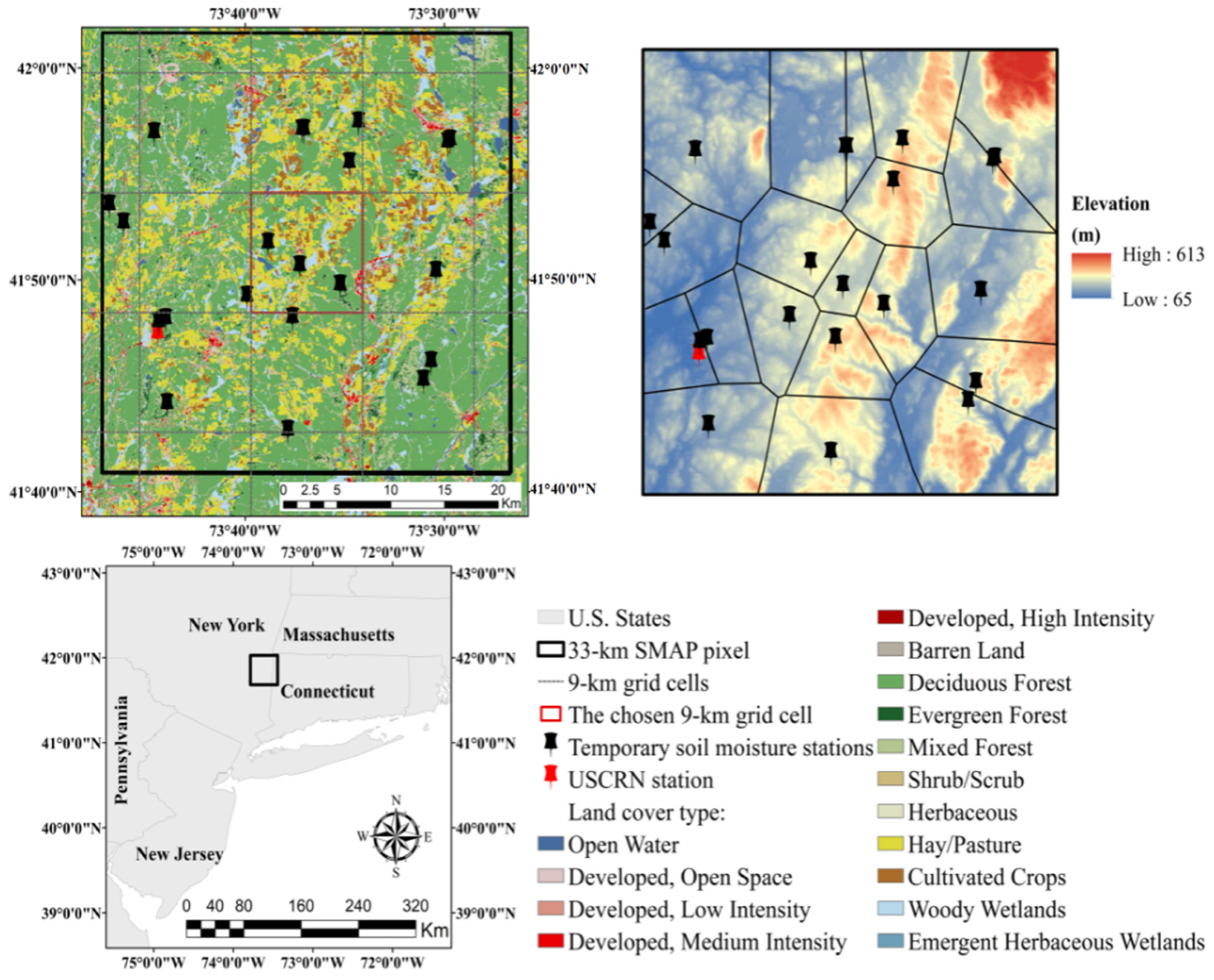The site covers an area of 30 km by 40 km [32]. The area of interest in this study is aligned with the 33-km SMAP grid cell (Figure 1). MB was selected as a representative site of the Northeastern US temperate forests since it is approximately 65% forested and 23% pasture or hay fields, as classified by the National Land Cover Database (NLCD). The forested sites fall under three main categories: deciduous forest, mixed forest, and evergreen forest, covering approximately 53%, 5%, and 2% of the total grid cell area, respectively, as mapped by NLCD. Within the SMAP 33-km grid cell, there are oak-hickory, beech-maple, and coniferous forests representing approximately 30%, 30%, and 4% of the total grid cell area, respectively [31,32]

The MB site has been equipped with a temporary soil moisture network containing 25 stations for the purpose of collecting ground-based soil moisture, soil temperature, and air temperature measurements starting in May 2019 [33]. Soil moisture measurements were collected at three different depths. The first layer of soil is measured from 0–5 cm in depth (the top layer), followed by a second layer of soil measuring from 3–7 cm and a third layer measuring from 8–12 cm. As for the top layer, the soil moisture sensor is top-down, while the sensors for the other two layers/depths are installed horizontally [33]. It is important to note that the sensors at the Millbrook site have not been site-specifically calibrated and the values are based on the generic factory calibration. Moreover, the soil moisture measurements collected when the soil temperatures were less than 4 °C were excluded due to potential errors introduced by the soil freeze\thaw fluctuations. Thus, data collected during December, January, and February were not used in the analysis.

This study is also interested in assessing soil moisture variability over a longer period compared to previous studies. Consequently, the upscaled soil moisture values were only calculated when data from all stations were available. Stations with significant gaps in coverage were excluded from the analysis. The analysis was carried out using the remaining 21 soil moisture stations.

2.2. SMAP Soil Moisture Data Product

SMAP data products include instrument measurements (Level 1), geophysical retrievals (Levels 2 and 3), and land surface models (Level 4). A series of 36-km, 9-km, and 3-km (nested) Equal-Area Scalable Earth version 2 (EASE-2) grids is used for these products. The radiometer-based products provide soil moisture information generated through three algorithms: single-channel vertical polarization (SCA-V), single-channel horizontal polarization (SCA-H), and dual-channel algorithms (DCA). The SMAP brightness temperature (TB) measurements have a 38-km resolution, and the measurements are filtered to eliminate radio frequency interference [34]. On the 9-km grid, soil moisture is sampled using the enhanced TB product. Due to the large spatial resolution of the TB measurement, TB from a 9-km grid cell is converted into soil moisture estimates using ancillary data for a 33-km aggregation domain centered on the 9-km grid cell, thereby approximating the spatial resolution of the TB measurement [35].

It is important to note that the SMAP soil moisture product is resampled to a fixed Earth grid that facilitates its use in applications. In this study, the 33-km SMAP enhanced level 2 soil moisture passive (L2SMP_E) product was used [35]. The assessment of the L2SMP_E product is performed for the nominal contributing domain (33-km) rather than the nesting grid cells (9-km). Colliander et al. (2018) investigated the differences between spatial resolution and grid size for the L2SMP_E under the assumption that the spatial resolution equals the 9-km grid size [36]. Results from their work showed that the impact of validating the 9-km grid product with in-situ data collected over a 9-km versus a 33-km domain was very small over homogenous sites. The current study investigates the accuracy of the L2SMP_E over a heterogeneous site, meaning that the soil moisture interpolated at the 9-km pixels may not properly represent the soil moisture measured within the satellite footprint. Thus, it is critical to use the native product resolution, i.e., 33 km, prior to its spatial smoothing to generate the 9-km product, especially over heterogeneous sites. Figure 1 illustrates the chosen 9-km cell location that corresponds to the depicted 33-km domain.

On the other hand, microwave instruments’ ability to detect soil moisture is dependent on the distribution and content of soil moisture. As a result, the mission decided to specify the products to provide a soil moisture estimate for the top 5 cm of the soil column to account for this effect in the data product.

In order to meet the mission requirement for surface soil moisture, the products must have an unbiased root mean square difference of 0.04 m³.m⁻³ within the retrieval area when the vegetation water content is less than 5 kg m⁻² [3]. The SMAP satellite is in a 6 AM/6 PM sun-synchronized high-inclination orbit and undertakes measurements in the mornings and evenings. The focus of this study is the assessment of SMAP AM observations, in accordance with the SMAP mission priority [12]. Nevertheless, PM overpasses are also considered, and a comparison was made between the accuracy of the SMAP AM and PM overpasses.

Note that SMAP soil moisture measurements in regions with canopy vegetation water content greater than 5 kg m⁻² are denoted as flagged data and are considered unreliable due to high vegetation water content [12]. However, this study intends to examine the accuracy of SMAP in forested regions. Accordingly, the SMAP quality flags were not applied in this study (similar to the study detailed in [37]).

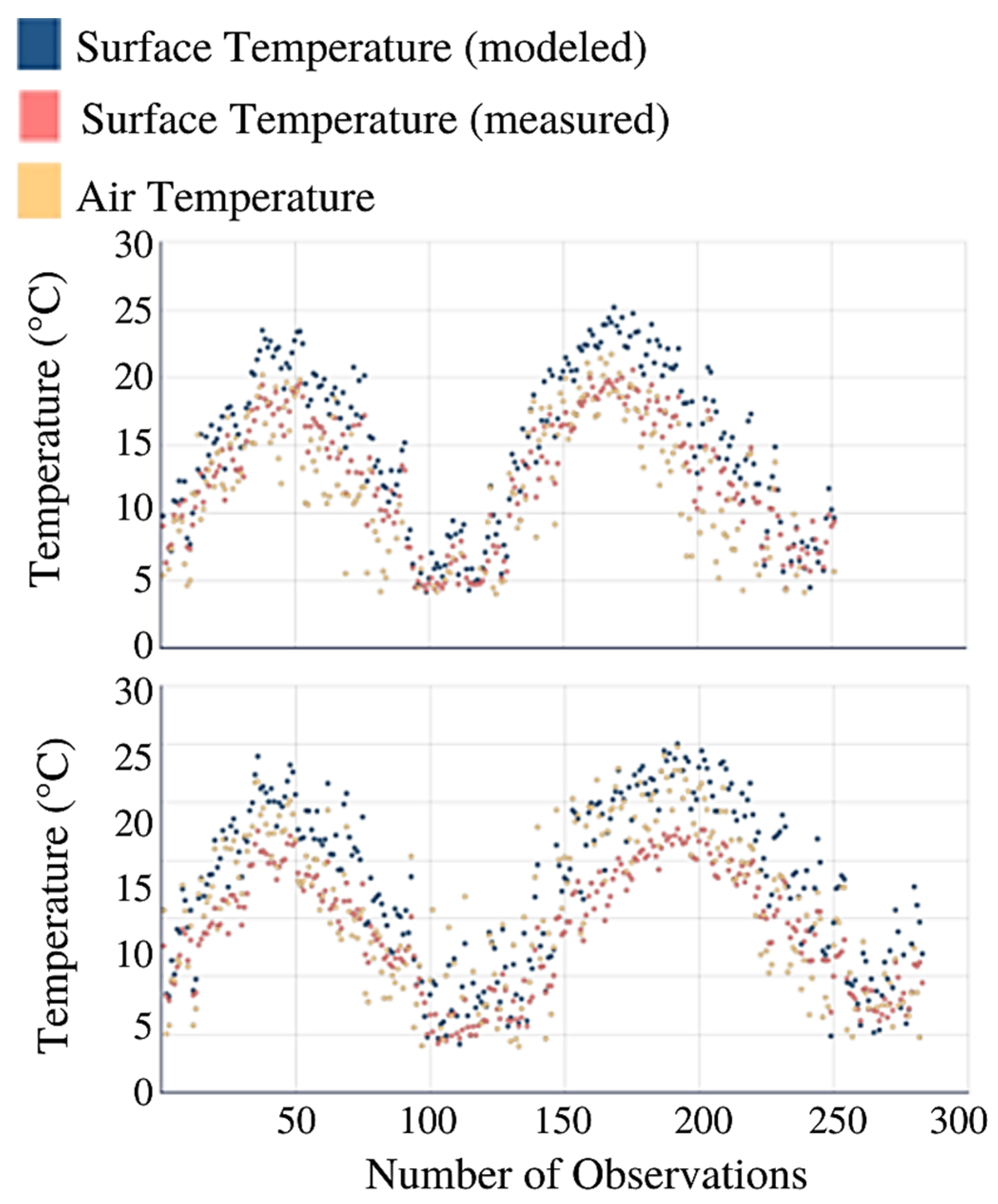
Along with the AM/PM soil moisture observations, the effective soil temperature used for the soil moisture retrievals was obtained from the SMAP SM product and compared to the measured soil and air temperatures (Figure 2). It is important to mention that the effective soil temperature is one of the dynamic ancillary data that is used in the soil moisture retrieval process.

Measurements of surface and air temperatures at the exact overpass (AM/PM) time were collected from the site stations and the arithmetic average of each variable was computed. It is important to mention that the considered temperature observations correspond to the filtered in situ soil moisture series. Thus, temperatures below 4 °C are not represented in Figure 2. The scatter plot shows that the modeled data used for SM retrieval at the AM and PM overpasses has substantial differences to the measured soil temperature depending on the season and overpass timing. During the summer AM overpasses, the modeled temperature is higher than the soil and air temperatures by up to 5 °C. The air and soil temperatures are overall similar, but there are also large day-to-day differences, and the differences increase towards fall. During the shoulder seasons, the differences tend to be overall smaller. During the summer PM overpasses, the modeled temperature is higher than the soil temperature by up to 10 °C. The modeled temperature is overall close to the measured air temperature. During the shoulder seasons, the differences tend to get smaller, similarly to the AM case.

2.3. Vegetation Data

The retrieval of soil moisture includes a wide range of static ancillary data, including permanent masks, topography, water fractions, surface roughness, soil types, and dynamic ancillary data, such as land cover precipitation, vegetation parameters, and effective soil temperatures [12]. The SMAP soil moisture retrieval algorithm involves the modeling of the vegetation effect using historical data of the NDVI. Specifically, the SMAP algorithm uses a vegetation optical depth value based on the NDVI information provided by MODIS.

For forested regions, it is challenging to determine the vegetation optical depth at L-band due to the dielectric properties of the branches and dense clusters of leaves. Previous studies have examined forest vegetation optical depth at the L-band frequency range from the perspective of spatial distribution [38,39,40,41,42]. Nevertheless, there is still a need for further research into the temporal variation of vegetation optical depth in forest ecosystems, especially during the wet and dry seasons. Further, the soil and canopy temperatures are assumed to be equal in the SMAP retrieval algorithm at the SMAP overpass time, but as Figure 2 shows, this assumption may not work well for forests. The issue is exacerbated by the large emissions caused by vegetation [43].

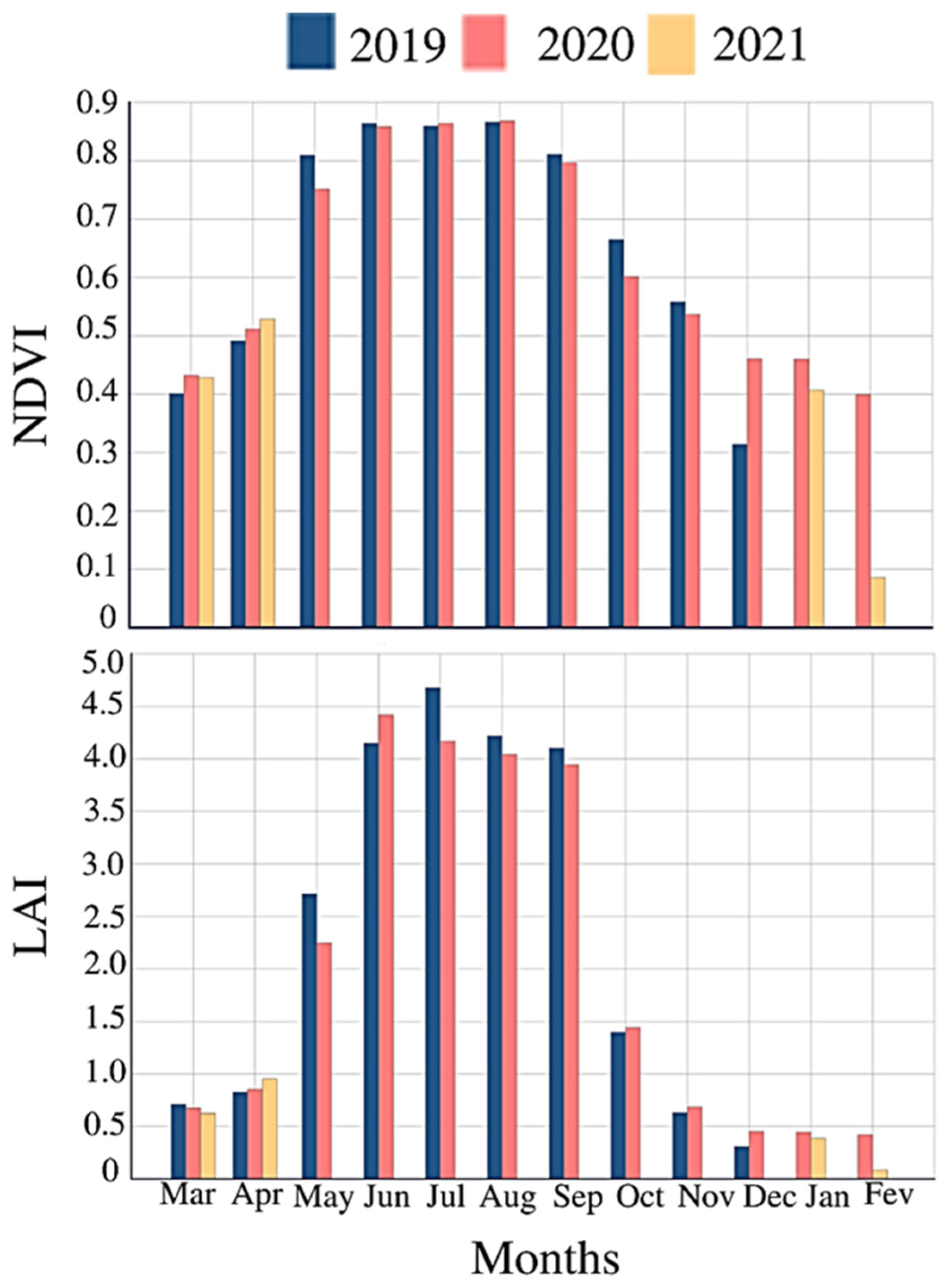
The SMAP soil moisture retrieval using passive microwave data use the τ-ω model in which the vegetation scattering effect is characterized by the scattering albedo (ω) whereas the attenuation effect is characterized by the vegetation optical depth (τ). The SMAP algorithm represents vegetation and surface emission, which are both impacted by the overlying canopy through attenuation and scattering losses characterized by the parameters τ and ω; therefore, the estimation of SM is sensitive to the values of τ and ω. In forested ecosystems, the seasonal variability of vegetation is expected to be reflected in its effect on the retrieval of soil moisture. This is critical, especially if the contribution of forests in the radiative transfer model is not properly accounted for. In this study, the potential impact of changes in vegetation cover on the performance of soil moisture retrieval is assessed. The variability of vegetation cover over the Millbrook site was studied by analyzing time series of the Normalized Difference Vegetation Index (NDVI), and Leaf Areal Index (LAI), spanning the period of 1 April 2019 to 30 April 2021, that were obtained from 16-day MODIS NDVI (MOD13A1) and 4-day MODIS LAI (MCD15A3H) imagery, respectively.

Figure 3 presents information about vegetation density and vitality at the Millbrook site during the experiment period. NDVI values revealed a significant seasonal change in the vegetation corresponding to an increase during the spring leaf development season and further maturation of the canopy, and correspondingly, a decrease during the autumn senescence season was observed. For instance, NDVI values peaked between the months of May and September within a range of 0.75 to 0.86. NDVI values declined throughout October and November due to leaf abscission, reaching their lowest values during January–February when all leaves had fallen from deciduous trees and were completely absent in the considered area (Figure 3). Similarly, LAI peaked during the months of June–September and dramatically declined during the months of October and November. In spring and summer, the LAI increased significantly, reached its peak value (greater than 4) in mid-summer, and then gradually decreased in autumn (Figure 3). In autumn, the canopy decreased, reflecting the trajectories of leaf abscission. Overall, LAI and NDVI exhibit the seasonal cycle of the tree phenology, but the relative magnitude of the cycle is larger for LAI, and its autumn decrease is steeper and occurs earlier than that of NDVI.

2.4. Soil Moisture Upscaling Methods

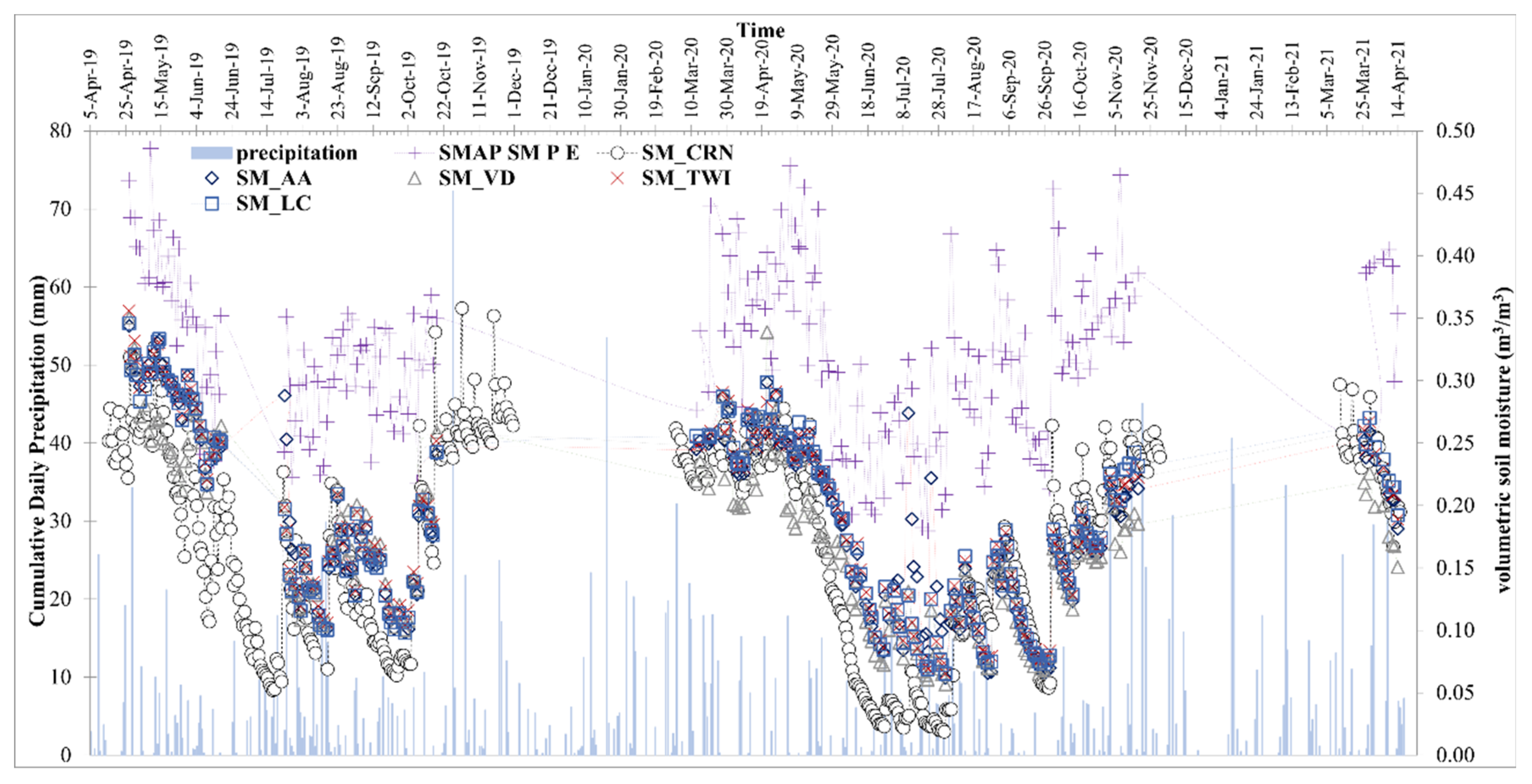
To assess SMAP soil moisture accuracy over the SMAP 33-km grid cell, data from the temporary stations were upscaled using four different upscaling methods. Prior to upscaling, in situ soil moisture observations from 21 stations were collected between 6:00 AM/PM and 7:00 AM/PM, local time, and the arithmetic mean soil moisture was calculated as a representative measurement that is close to the satellite overpass time. Nevertheless, it is not expected that soil moisture varies significantly within the one-hour window. Further, the collected measurements were checked for missing data and outliers (spikes, out-of-range values, and sudden drops) [44]. Based on a quality assessment of the measured soil moisture time series, 21 stations were selected as point-based measurements (see Section 2.1). The number and geographical distribution of sensors within the studied grid cell are in accordance with the recommendations concerning the validation process of SMAP products [14].

To spatially upscale the soil moisture in situ measurements, a weight is assigned to the soil moisture time series recorded by the soil moisture stations. Physical and geostatistical factors were incorporated into the upscaling process in order to account for the spatial variability of soil moisture. The study examines two upscaling approaches based on physical parameters (topo-graphic wetness index and land cover), a geostatistical approach based on the Voronoi diagram, and an arithmetic method.

In this study, four different upscaling methods are employed: arithmetic average, Voronoi diagram, topographic wetness index (TWI)-, and land cover-based weighted average. For the arithmetic average approach, the arithmetic mean is computed for stations within the 33-km pixel. For the Voronoi diagram approach, the area incorporating the measurement locations is divided into polygons so that the polygon around each location consists of an area that is as close as or closer to the location than any other measurement location in the area. Based on the surface areas of the polygons, weights are assigned to soil moisture stations.

For the TWI-based upscaling approach, the physical characteristics of the regions determine the weights of each station. The technique measures the topographic influence on hydrological processes by combining the local contributing area and slope. In this study, the TWI was computed based on a digital elevation model (DEM) of the site and calculations of the upslope area, creek cell representation, and slope were performed in accordance with the recommendations of Sorensen et al. (2006) to better estimate soil moisture spatial variability [45]. The TWI intervals within the 33-km pixel were calculated by using a histogram. Subsequently, each station was attributed to the corresponding interval based on its TWI value. Accordingly, each station was assigned a weight based on the weight of the interval to which it belonged.

For the land cover-based approach, the soil moisture stations were clustered according to the land cover features of their respective locations. The in situ soil moisture values for each cluster within the study area were weighted according to the percent area of the land cover type within the study area. Thus, the weight of each station is proportional to the percent area of each land cover type within the 33-km pixel.

2.5. Validation Metrics

The assessment of the temporal variability of SMAP soil moisture retrieval accuracy was conducted using the daily soil moisture time series. The upscaled soil moisture time series has been rearranged into 12 series, each representing daily soil moisture values for a particular month. In this study, the accuracy of SMAP products has been assessed via statistical metrics presented in [3]. The SMAP soil moisture data were compared to upscaled in situ measurements using MD, ubRMSD, and RMSD.

The MD represents the systematic difference between the satellite retrievals (S_s) and in situ measurements (S_m) and can effectively evaluate the overall level of bias between the considered variables. The MD is defined as:

$$\mathrm{MD}=\frac{{{\displaystyle \sum }}_{i=1}^N\left(S_s-S_m\right)}{N}$$

(1)

On the other hand, the RMSD measures the differences between the estimated SM values from SMAP and the ground based measured values. The RMSD represents the square root of the second sample moment of the differences between the estimated values and the upscaled soil moisture measurements. The RMSD can be calculated as follows:

$$\mathrm{RMSD}=\sqrt{\frac{{{\displaystyle \sum }}_{i=1}^N{\left(Ss-Sm\right)}^2}{N}}$$

(2)

The ubRMSD is an unbiased metric that evaluates the reliability of surface soil moisture. The ubRMSD can be calculated using the following formula:

$$\mathrm{ubRMSD}=\sqrt{{\left(\mathrm{RMSD}\right)}^2-{\left(\mathrm{MD}\right)}^2}$$

(3)

3. Results

3.1. Comparison between SMAP Observation and In Situ Measurements

A temporal analysis of the accuracy of SMAP soil moisture was conducted by comparing the soil moisture data acquired from satellite and ground-based observations between April 2019 and April 2021. The upscaled soil moisture values obtained from the temporary network were compared with soil moisture observations obtained from one U.S. Climate Reference Network (USCRN) station deployed within the 33-km SMAP pixel. Data from the USCRN are quality controlled, and observations from the site and the network, in general, are reliable. The purpose of the comparison was to understand the seasonality of soil moisture at the site and to verify the consistency of the upscaled soil moisture measurements from the temporary network with USCRN soil moisture. Figure 4 displays the upscaled and the USCRN soil moisture time series. It was determined that the temporal evolution of upscaled soil moisture from the temporal network agrees well with soil moisture records from the USCRN station as they both show the same seasonal variability. The records from the USCRN station are employed to comment on soil moisture variation and compare the general pattern of soil moisture variation from SMAP observations and the upscaled in-situ measurements. It is important to note that soil moisture records from USCRN stations during frozen conditions of soil are not considered.

Four distinct phases were observed in the soil moisture time series (Figure 4). Between March and April, one can observe a moist plateau phase distinguished by relatively high soil moisture values within a 0.18–0.34 m³.m⁻³ range and an average soil moisture value of ~0.25 m³.m⁻³. During the period between late May and June, there is a transitional drying phase characterized by a decrease in volumetric soil moisture values within a 0.10–0.31 m³.m⁻³ range and an average soil moisture value of 0.22 m³.m⁻³. A dry phase occurs from late June through early-August, and soil moisture values are within a 0.06–0.20 m³.m⁻³ range and average soil moisture value of 0.11 m³.m⁻³. Both the field and SMAP observations show a significant decrease in volumetric soil moisture values during this period. However, a fluctuation in soil moisture values is observed due to the occurrence of rainfall events. The surface soil moisture at the Millbrook site undergoes a recharge period from mid-September to late October. During the recharge period, soil moisture values varied within a 0.07–0.24 m³.m⁻³ range, and the average soil moisture value was around 0.14 m³.m⁻³.

It is essential to mention that the precipitation series shown in Figure 4 were obtained from the USCRN station located at the southwest corner of the grid cell (Figure 1). Therefore, using point-based rainfall measurements may result in a failure to capture the spatial variability of rainfall over the study area. Overall, the upscaled soil moisture time series and USCRN measurements are responsive to precipitation events as they both show a sharp increase right after the occurrence of a rainfall event. Nevertheless, Figure 4 shows a systematic overestimation of soil moisture in the SMAP values when compared to the upscaled values. The discrepancies, however, between SMAP soil moisture and ground observation seem to be season dependent. The gap during the summer months, from June to August, is the highest compared to the rest of the year, with a smaller gap in the winter and spring months, suggesting that the performance of SMAP retrievals is also subjected to seasonal variability, which could be attributed to changes in surface and vegetation conditions.

Figure 5 presents the SMAP AM/PM observations, the minimum and the maximum recorded soil moisture values from the site stations for the considered time steps. It is important to mention that approximately 90% of the maximum recorded soil moisture was obtained from a station located at the center of the grid cell where the deciduous forest land cover is dominant. The measured soil moisture values and the SMAP retrievals have the same patterns. The SMAP values are systematically close to the maximum recorded soil moisture from the site stations. This finding is valid for both the ascending and descending overpass observations.

Figure 6 shows the correlations between the upscaled in situ soil moisture (arithmetic average, Voronoi diagram, TWI-weighted, and land cover-weighted) and the SMAP soil moisture. The correlations are similar regardless of the upscaling method. The correlation values ranged from 0.68 to 0.71 and 0.71 to 0.74, for the AM and PM overpasses, respectively. The soil moisture series derived from the TWI showed marginally better correlation values for both the ascending and descending observations. The correlation values are generally lower than those obtained in the previous validation studies conducted using CVS [19]. This could be attributed to the low covariance between the SMAP and the in-situ soil moisture, especially during the spring–summer transition as the SMAP soil moisture fails to capture the short-term variation in soil moisture as reported in Figure 4.

Figure 6 shows that the normalized standard deviations of upscaled soil moisture time series are in close agreement with each other. Additionally, the normalized RMSD displayed similar patterns between the upscaled time series and the SMAP series. These results indicate that the upscaling methods result in very similar soil moisture values when applied to the Millbrook site. In part, the consistency among the upscaling approaches may be explained by the fact that the ground-based sensors were placed in forested and open areas and were well distributed in space [19]. Therefore, the spatial heterogeneity and covariance of soil moisture are well captured by the stations within the SMAP grid cell, and there is little additional value that the upscaling methods can provide.

3.2. Temporal Variation of the Retrieved Soil Moisture Accuracy

The assessment of the temporal variability of the performance of the SMAP L2SMP_E AM/PM retrievals was conducted by computing the monthly MD, ubRMSD, and RMSD throughout the study period. The evaluation metrics are presented as bar charts in Figure 7, Figure 8 and Figure 9, using soil moisture time series from the L2SMP_E product and the upscaled in situ measurements.

Figure 7 shows the L2SMP_E soil moisture assessment with the MD statistic. The MD results showed persistent positive values throughout the study period, indicating that the SMAP retrievals are systematically overestimating the in situ observations for the different seasons (Figure 4), corroborating the qualitative interpretation of the gap between the time series as displayed in Figure 4. During the various months of the year, errors associated with L2SMP_E varied greatly. Positive MD values were observed throughout the evaluation period, which is consistent with the graphical comparison of time series. In general, the error of the L2SMP_E data was greater during the period of July–October. For the month of August, L2SMP_E MD values ranged from 0.166 to 0.171 m³.m⁻³ for the AM overpass and 0.182 to 0.188 m³.m⁻³ for the PM overpass. During the months of March–June, more accurate soil moisture estimates were obtained with a substantial decrease in MD values. From the results of the different upscaling methods, the average MD values for the AM overpass for March, April, May, and June were 0.10 m³.m⁻³, 0.12 m³.m⁻³, 0.12 m³.m⁻³, and 0.09 respectively. On the other hand, the average MD values for the PM overpass for March, April, May, and June were 0.15 m³.m⁻³, 0.15 m³.m⁻³, 0.16 m³.m⁻³, and 0.11, respectively. The results showed that higher MD values are observed when the vegetation is fully developed (July–September from Figure 2), and gradually decrease during the late winter and early spring.

Figure 8 illustrates the temporal variation of ubRMSD computed for the L2SMP_E soil moisture product over the course of the study period. Figure 8 shows that L2SMP_E’s accuracy for an area with prevailing deciduous forest land cover type is significantly affected by the vegetation seasonal variations, which tend to degrade the retrieval. Most of the monthly ubRMSD values exceeded the SMAP mission requirement (ubRMSD 0.04 m³.m⁻³), particularly over the period from March to June and October–November for the AM overpass observations and March–May and November for the PM overpass observations.

In contrast, L2SMP_E data showed good performance for July, August, and September with an average ubRMSD of 0.03 m³.m⁻³ for both the ascending and descending observations, which does not exceed the SMAP mission requirements. Results indicated that the highest performance of SMAP soil moisture retrievals occurred during July, with an average ubRMSD value of 0.03 for both the AM and PM overpass. This finding is valid for the four upscaling methods. During March-June, the agreement with in situ observations in terms of ubRMSD degraded, with ubRMSD values reaching ~0.06 m³.m⁻³ in March. The differences between the different upscaling methods were not substantial. However, it is worth noting that the PM soil moisture series obtained from the TWI-based upscaling for the month of March is significantly lower with an ubRMSD value of 0.03 m³.m⁻³. An important factor lowering ubRMSD during the summer months is the overall lower soil moisture levels, which affect the ubRMSD values. The low ubRMSD values suggest that SMAP data could be reliably used for assessing the temporal variability of soil moisture in forested regions during part of the year. Retrievals that are conducted between the months of March–June should be used with more caution.

RMSD values (Figure 9) indicate that L2SMP_E performance is not stable and exhibits substantial variability throughout the various months of the year. In July, August, September, and October, we observed high RMSD values, ranging from 0.112 to 0.181 m³.m⁻³ and 0.181 to 0.202 m³.m⁻³ for the AM and PM overpasses, respectively. In July–October, there were no significant differences between the RMSD values obtained from the various upscaling methods. The L2SMP_E data is generally better from March through June, with the lowest RMSD values obtained during June. According to the results of the different upscaling methods for the AM and PM overpasses, the average RMSD value for June was 0.10 m³.m⁻³ and 0.16 m³.m⁻³, respectively. Overall, RMSD values were high during the summer season and gradually decreased during early spring. It is essential to mention that the different upscaling approaches exhibited similar RMSD patterns.

The ancillary data used for soil moisture retrievals have a significant impact on the accuracy of the estimated soil moisture. For instance, surface and vegetation temperatures play a critical role in estimating soil moisture, especially in forested sites. In the SMAP retrieval algorithm, both surface and vegetation temperatures are assumed to be equal. Thus, for forest vegetation characterized by dense canopy and leaf cover, a significant difference between soil and canopy temperatures may exist. A comparison between the modeled surface temperature used in SM retrievals and the surface and air temperature from the site stations was performed. The correlation, Mean Bias Error (MBE), and Root Square Error were computed, and the results are summarized in

Table 1. Comparison between the modeled surface temperature used for SM retrievals and the measured surface and air temperature.

			In Situ Surface Temperature			In Situ Air Temperature
			R	MBE (°C)	RMSE (°C)	R	MBE (°C)	RMSE (°C)
Effective Temperature	March	AM	0.79	−0.36	1.11	0.27	−5.25	6.18
		PM	0.87	−2.47	2.97	0.48	−1.54	3.134
	April	AM	0.85	−0.92	1.21	0.34	−4.46	5.48
		PM	0.85	−2.33	2.94	0.48	−2.43	3.90
	May	AM	0.97	−1.73	1.9	0.68	−2.29	3.33
		PM	0.96	−3.69	4.07	0.85	−0.92	2.31
	June	AM	0.93	−3.04	3.13	0.43	−2.54	3.35
		PM	0.89	−5.85	5.96	0.78	−0.95	1.71
	July	AM	0.89	−4.00	4.05	0.41	−3.77	4.01
		PM	0.82	−6.25	6.30	0.76	−2.01	2.38
	August	AM	0.85	−3.94	3.99	0.365	−5.43	5.83
		PM	0.83	−5.67	5.74	0.82	−3.47	3.66
	September	AM	0.94	−3.49	3.53	0.52	−6.45	7.03
		PM	0.78	−5.81	5.32	0.78	−4.87	5.16
	October	AM	0.92	−2.26	2.36	0.40	−6.28	6.76
		PM	0.85	−3.17	3.47	0.578	−4.58	5.04
	November	AM	0.97	−0.66	1.19	0.24	−5.39	7.1
		PM	0.83	−1.70	2.95	0.84	−2.35	3.138
	Overall	AM	0.99	−2.42	2.84	0.87	−4.67	5.64
		PM	0.98	−4.05	4.60	0.93	−3.06	3.69

.

The overall correlation results showed excellent agreement between the modeled and collected data. Thus, surface temperature is capable of detecting the temperature temporal variation in forested ecosystems. On the other hand, MBE and RMSE values showed a significant difference between the modeled and observed soil temperature data, especially for the PM overpass. In addition, the difference between air temperature and the modeled surface data is also significant, and assuming an equal temperature for the surface and canopy may increase the error of the SM product.

As shown in Table 1, negative MBE was obtained for effective temperature for the evaluated months. Negative MBE values are present for the morning and evening soil temperature measurements. The obtained results suggest that the model-based effective soil temperature is higher than the real soil temperature. However, it is important to mention that more significant MBE values are observed for the PM measurements. The highest MDE values were observed during the warm season (June–August) where MBE values varied between −3.04 and −4.00 °C, and −5.67 and −6.25 °C for the AM and PM date, respectively. Thus, such a discrepancy may affect the retrieved soil moisture and lead to a wet bias.

The modeled temperature demonstrates a strong correlation with in situ surface measurements with an R > 0.79. On the other hand, correlation results for the modeled temperature and in situ air temperature exhibit poor R results for the AM data. The poor correlation was primarily observed during March–May, when short-term variations in temperatures may be associated with the transition from the cold season to the warmer season.

The monthly RMSE values show that the performance of the modeled temperature data is relatively stable for the evaluated months. However, higher RMSE was observed for the PM surface temperature data. Overall, higher RMSE values were observed during June–September. The resulting discrepancy may contribute to the variation of the retrieved soil moisture accuracy.

4. Discussion

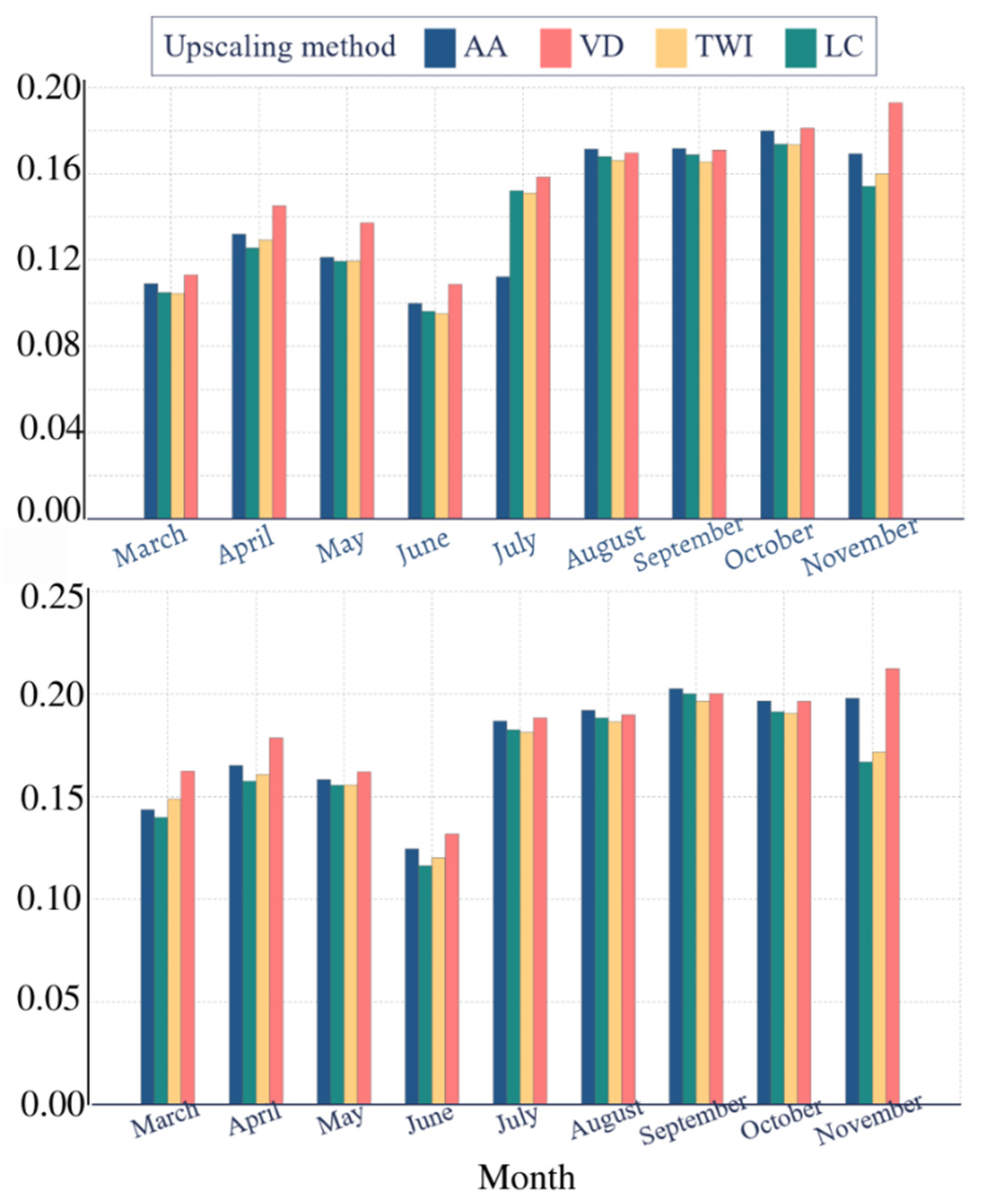
This study investigated the spatiotemporal accuracy of L2SMP_E, a remotely sensed soil moisture product, over a deciduous forest region. The error associated with the soil moisture retrievals was obtained by computing error metrics between the L2SMP_E series and in situ soil moisture measurements upscaled with four different methods. SMAP adopted the Voronoi Diagram method over most of the CVS to upscale in situ observations and assess the performance of satellite retrievals [19]. The results show that the method leads to a comparable outcome when compared to the other upscaling methods. Thus, no significant improvements in error statistics were obtained while validating the L2SMP_E product with alternative upscaling approaches. This can be explained by the uniform distribution of the network over the site and the dominance of the deciduous forest land cover type over the site (~65%). The similarities in the comparison among the upscaling methods can also be attributed to the uniformity of other landscape parameters, such as the dominance of high-rock-fraction soils over the experiment site. This finding is also in line with the outcomes of SMAPVEX16 that was conducted in Canada over one of the SMAP core validation sites that are dominated by annual cropping, which has a lower effect on the SMAP signal compared to the Millbrook forest land cover [17]. The consistency among the upscaling methods over the two sites with different land cover conditions suggests that the selection of the upscaling technique may not have a large effect on the assessment of the SMAP performance throughout the seasons. Other sites with different land cover conditions may be considered in future work to corroborate this finding.

The results are site-specific as the weights used in the upscaling methods depend on the locations of the sensors, the density of their spatial distribution within the grid cell, and their organization with respect to the different land cover types and changes in topography. Expanding the study, in future work, to other sites with different land cover classes and network densities is necessary to corroborate the findings. Nevertheless, this study underlines the importance of an optimal spatial sampling of soil moisture within heterogeneous grid cells, especially, in the presence of forests and dense vegetation where SMAP accuracy degrades due to the compounded effect of vegetation scattering and water content. This is particularly important in temperate weather regions like Millbrook, where the vegetation evolves in time and hence its effect on the SMAP performance. An optimal distribution of stations within the grid cell that accounts for land cover (i.e., vegetation) and topography may compensate for the degradation of the retrieval over vegetated areas and report a more representative value of upscaled soil moisture.

The heterogeneity of the study site is the main driver of the variability of the in situ observations within the grid cell. As illustrated in Figure 1, the network of in situ sensors captures the spatial variability of the relief and the land cover, two main factors which control the distribution of soil moisture. With respect to topography, it is well understood that the lowest points in the domain are more suitable to drain the surface water and, therefore, tend to have higher soil moisture values. In addition to their elevation, the orientation of the grid cells expressed in terms of their topographic aspect plays a key role in the control of soil moisture as well [46,47]. The orientation of the hillside determines the amount of net radiation at the surface and the duration of exposure to sunlight, and therefore determining the distribution of latent heat and soil moisture. At the macroscale, the radiative interactions between the existing hills and mountains within the study domain could also impact surface emissions, brightness temperatures, and soil moisture values. Land cover also has a strong influence on the distribution of soil moisture. In the case of the Millbrook site with the prevailing forest land cover type, the density of the canopy can control, with its shading effect, the amount of illumination that reaches the surface. The lower the amount of total irradiance at the surface, the higher the soil moisture. This could be reflected in the in situ observations but not necessarily the satellite ones as the signal may not reach the surface due to the opacity of the canopy. In addition, the heterogeneity of the land cover could introduce a variability in the surface emissivity in the thermal and microwave domains, which directly controls skin temperature and its relationship with brightness temperature, especially over bare soil areas.

The variability of the performance of SMAP retrievals throughout the seasons can be attributed to the change in the vegetation phenology and the soil and vegetation temperature profiles and their impact on the estimation of the vegetation optical depth and the effective temperature that are used in the retrieval of soil moisture. The effective temperature is the temperature of the soil moisture layer from which the passive microwave signature originates. The depth of the layer depends on the frequency used and the vertical moisture distribution. For the SMAP L-band frequency, the depth that is commonly used is 5 cm. Temimi et al. (2014) showed using in situ observations from a ground-based L-band radiometer that the penetration depth of the signal can reach 12 cm [31]. The temperature profile along that depth tends to vary seasonally and diurnally depending on the amount of radiation at the surface. With lower net radiation at the surface during winter, the temperature profile would tend to be more uniform. However, as net radiation increases during the summer months, one should expect a non-uniform temperature profile with a higher temperature at the upper part of the soil layer near the surface, which should rapidly decrease at the deeper part of the same soil layer. The non-uniform distribution of soil temperature along the profile makes the estimation of the effective temperature, which should be representative of the entire layer, more challenging during warm months than clod ones.

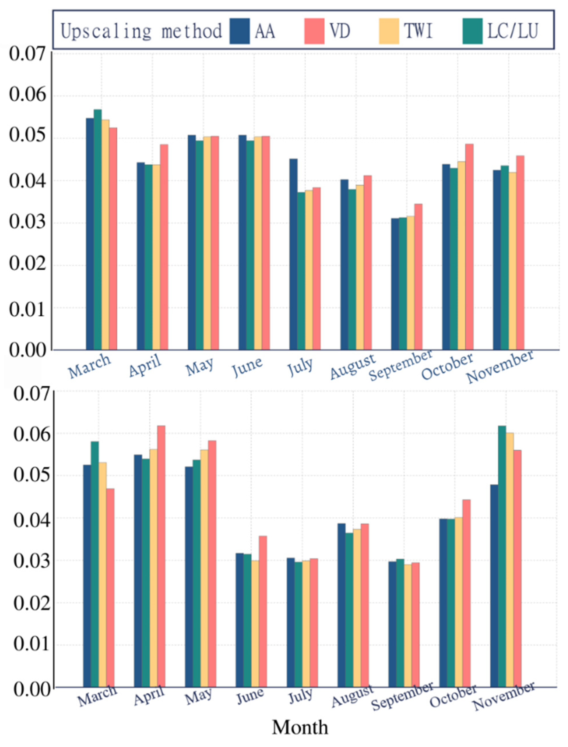
The analysis captured the seasonal variations of the SMAP performance. For instance, SMAP retrievals performed well during July-September in terms of ubRMSD, and poor performance with larger ubRMSD values was found during periods spanning March-June. Overall, the obtained ubRMSD values indicate that SMAP data can be used to assess the temporal variability (trend and seasonality) of soil moisture in forested regions. However, retrievals that are conducted between the months of March and June should be used with more caution. Therefore, a standardized soil moisture index can be derived from the SMAP data for drought monitoring and flood mitigation applications by identifying dry and wet periods of the year. It is noteworthy that the RMSD values obtained for the different months were higher than the ubRMSD values. Therefore, the monthly MD values were responsible for the total uncertainty (RMSD). SMAP accuracy in forested ecosystems may be improved by understanding the source and seasonality of MD. In addition, results indicated that the agreement between the in situ measurements and AM observations was higher than the PM observations. The sources of errors causing variations between the morning and evening soil moisture retrievals could be attributed to the assumption that the canopy temperature is equal to the air temperature and the computation of the effective soil temperature in a forested region.

Consequently, it is important to properly account for vegetation and its seasonality in the retrieval of soil moisture, which is in agreement with the recommendations provided by Colliander et al. (2020) [32]. By modeling the attenuation as a function of LAI instead of NDVI (as is done in the current SMAP algorithm), for example, the representation of the temporal variation of the attenuation in the τ-ω model can potentially be enhanced. An accurate characterization of the vegetation cover and its contribution to the microwave signal is essential to this endeavor, which can be accomplished by conducting intense field campaigns at forest sites such as Millbrook. To improve the retrieval of soil moisture under forest canopy, two intensive observation periods (IOP) are scheduled for April 2022 and July 2022 at Millbrook, and another site in Massachusetts, with a dominant forest cover [43].

5. Conclusions

It is important to accurately assess the performance of SMAP retrievals over forested regions, especially as the vegetation properties vary throughout the seasons. SMAPVEX19-22, which is being conducted in the region of Millbrook, New York, provided the opportunity to collect soil moisture measurements at deciduous forest sites. In this study, the level 2 enhanced soil moisture passive microwave product was compared to in situ soil moisture measurements collected from the network that is deployed in Millbrook. SMAP retrievals were evaluated using in situ soil moisture measurements, which were upscaled using four techniques, namely, arithmetic average, Voronoi diagram, TWI-weighted, and land cover-weighted. The difference between the various upscaling approaches was not significant, indicating that soil moisture conditions are sufficiently represented by the stations at the 33-km SMAP scale.

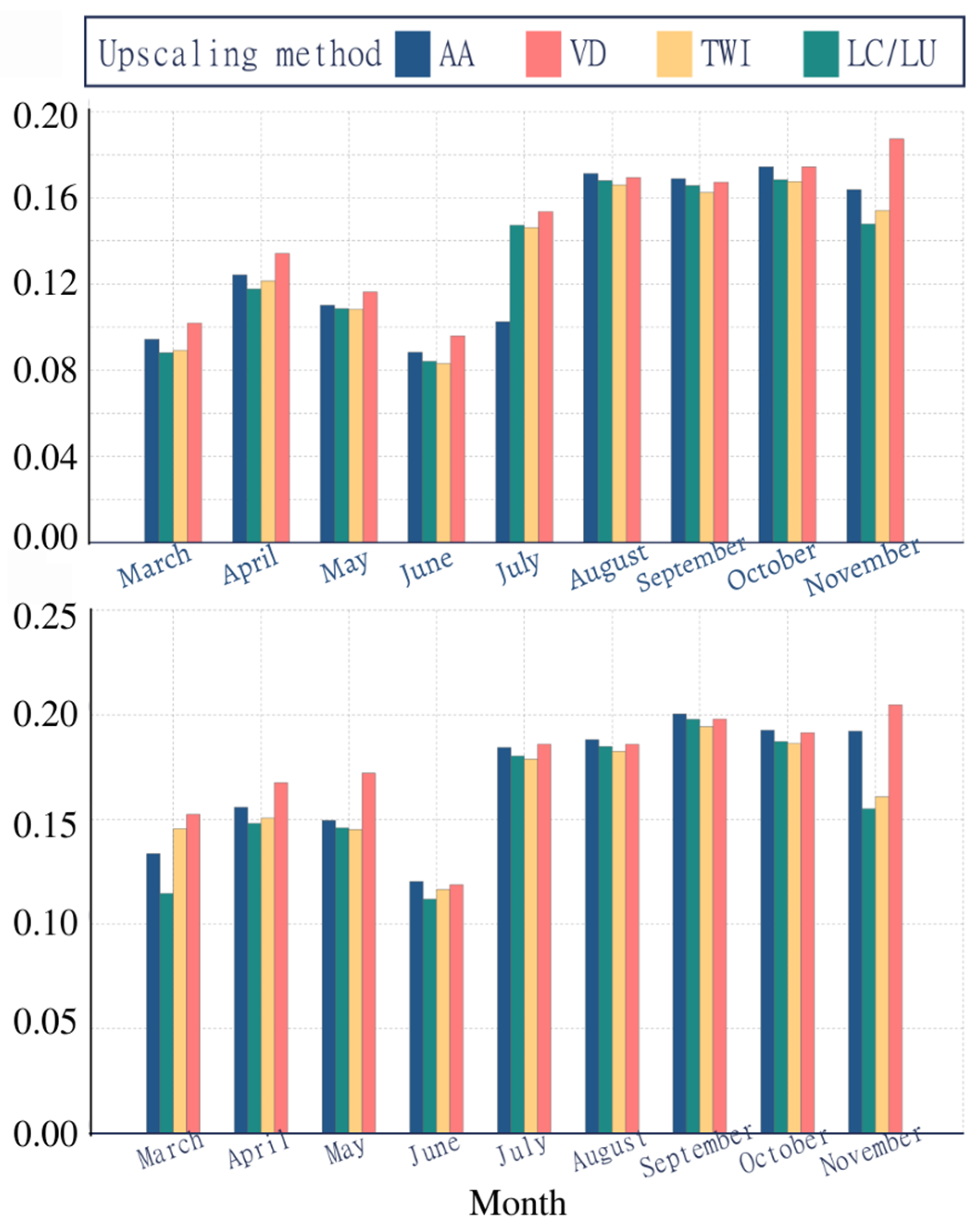
The temporal analysis revealed that SMAP retrievals achieved a reasonable level of sensitivity to changes in soil moisture during the different months of the year. Nevertheless, SMAP accuracy varied over time. During July–September, high-quality retrievals are obtained following bias removal (ubRMSD is generally less than 0.04 m³.m⁻³). During March–June, the agreement with in situ measurements decreased with ubRMSD values exceeding 0.04 m³.m⁻³, reaching a maximum of ~0.06 m³.m⁻³ in April. The MD, however, varied depending on the season in the range of 0.09–0.17 m³.m⁻³ for the AM overpasses and 0.12–0.20 m³.m⁻³ for the PM overpasses. The sources of errors that caused variation in the agreement between the soil moisture retrievals and ground-based measurements could be attributed to the challenging determination of the soil’s effective temperature. In the retrieval algorithm, the effective temperature of vegetation is assumed to equal the effective temperature of soil, which can introduce another source of error, particularly during the expansion and senescence of the canopy.

In this study, the possible sources of errors associated with SMAP retrievals over a forested area were discussed. Further studies are required to better understand the sensitivity of the TB measurements to seasonal variation in vegetation cover and to develop the characterization of the attenuation parameter in the τ-ω model.

References

1. Kumar, A.; Kumar, M.; Pandey, R.; ZhiGuo, Y.; Cabral-Pinto, M. Forest Soil Nutrient Stocks along Altitudinal Range of Uttarakhand Himalayas: An Aid to Nature Based Climate Solutions. CATENA 2021, 207, 105667. [Google Scholar] [CrossRef]
2. Humphrey, V.; Berg, A.; Ciais, P.; Gentine, P.; Jung, M.; Reichstein, M.; Seneviratne, S.I.; Frankenberg, C. Soil Moisture–Atmosphere Feedback Dominates Land Carbon Uptake Variability. Nature 2021, 592, 65–69. [Google Scholar] [CrossRef] [PubMed]
3. Entekhabi, D.; Reichle, R.H.; Koster, R.D.; Crow, W.T. Performance Metrics for Soil Moisture Retrievals and Application Requirements. J. Hydrometeorol. 2010, 11, 832–840. [Google Scholar] [CrossRef]
4. Douville, H.; Chauvin, F. Relevance of Soil Moisture for Seasonal Climate Predictions: A Preliminary Study. Clim. Dyn. 2000, 16, 719–736. [Google Scholar] [CrossRef]
5. Singh, G.; Das, N.N. A Data-Driven Approach Using the Remotely Sensed Soil Moisture Product to Identify Water-Demand in Agricultural Regions. Sci. Total Environ. 2022, 837, 155893. [Google Scholar] [CrossRef]
6. Hernández, A.J.; Lacasta, C.; Pastor, J. Effects of Different Management Practices on Soil Conservation and Soil Water in a Rainfed Olive Orchard. Agric. Water Manag. 2005, 77, 232–248. [Google Scholar] [CrossRef]
7. Dobriyal, P.; Qureshi, A.; Badola, R.; Hussain, S.A. A Review of the Methods Available for Estimating Soil Moisture and Its Implications for Water Resource Management. J. Hydrol. 2012, 458–459, 110–117. [Google Scholar] [CrossRef]
8. Ma, C.; Li, X.; Wang, S.; Wang, Z.; Che, T.; Jin, R.; Wang, W. Quantifying Uncertainties in Passive Microwave Remote Sensing of Soil Moisture via a Bayesian Probabilistic Inversion Method. IEEE Trans. Geosci. Remote Sens. 2022, 60, 1–18. [Google Scholar] [CrossRef]
9. Quets, J.; De Lannoy, G.J.M.; Al Yaari, A.; Chan, S.; Cosh, M.H.; Gruber, A.; Reichle, R.H.; Van der Schalie, R.; Wigneron, J.P. Uncertainty in Soil Moisture Retrievals: An Ensemble Approach Using SMOS L-Band Microwave Data. Remote Sens. Environ. 2019, 229, 133–147. [Google Scholar] [CrossRef]
10. Colliander, A.; Jackson, T.J.; Chan, S.K.; O’Neill, P.; Bindlish, R.; Cosh, M.H.; Caldwell, T.; Walker, J.P.; Berg, A.; McNairn, H.; et al. Seasonal Dependence of SMAP Radiometer-Based Soil Moisture Performance as Observed over Core Validation Sites. In Proceedings of the IGARSS 2019—2019 IEEE International Geoscience and Remote Sensing Symposium, Yokohama, Japan, 28 July–2 August 2019; pp. 5320–5323. [Google Scholar] [CrossRef]
11. Crow, W.T.; Berg, A.A.; Cosh, M.H.; Loew, A.; Mohanty, B.P.; Panciera, R.; De Rosnay, P.; Ryu, D.; Walker, J.P. Upscaling Sparse Ground-Based Soil Moisture Observations for the Validation of Coarse-Resolution Satellite Soil Moisture Products. Rev. Geophys. 2012, 50, 1–20. [Google Scholar] [CrossRef] [Green Version]
12. Entekhabi, D.; Njoku, E.G.; O’Neill, P.E.; Kellogg, K.H.; Crow, W.T.; Edelstein, W.N.; Entin, J.K.; Goodman, S.D.; Jackson, T.J.; Johnson, J.; et al. The Soil Moisture Active Passive (Smap) Mission. Proc. IEEE 2010, 98, 704–716. [Google Scholar] [CrossRef]
13. Reichle, R.H.; De Lannoy, G.J.M.; Liu, Q.; Ardizzone, J.V.; Colliander, A.; Conaty, A.; Crow, W.; Jackson, T.J.; Jones, L.A.; Kimball, J.S.; et al. Assessment of the SMAP Level-4 Surface and Root-Zone Soil Moisture Product Using In Situ Measurements. J. Hydrometeorol. 2017, 18, 2621–2645. [Google Scholar] [CrossRef]
14. Colliander, A.; Jackson, T.J.; Bindlish, R.; Chan, S.; Das, N.; Kim, S.B.; Cosh, M.H.; Dunbar, R.S.; Dang, L.; Pashaian, L.; et al. Validation of SMAP Surface Soil Moisture Products with Core Validation Sites. Remote Sens. Environ. 2017, 191, 215–231. [Google Scholar] [CrossRef]
15. Colliander, A.; Cosh, M.H.; Misra, S.; Jackson, T.J.; Crow, W.T.; Chan, S.; Bindlish, R.; Chae, C.; Holifield Collins, C.; Yueh, S.H. Validation and Scaling of Soil Moisture in a Semi-Arid Environment: SMAP Validation Experiment 2015 (SMAPVEX15). Remote Sens. Environ. 2017, 196, 101–112. [Google Scholar] [CrossRef]
16. Colliander, A.; Cosh, M.H.; Misra, S.; Jackson, T.J.; Crow, W.T.; Powers, J.; McNairn, H.; Bullock, P.; Berg, A.; Magagi, R.; et al. Comparison of High-Resolution Airborne Soil Moisture Retrievals to SMAP Soil Moisture during the SMAP Validation Experiment 2016 (SMAPVEX16). Remote Sens. Environ. 2019, 227, 137–150. [Google Scholar] [CrossRef]
17. Bhuiyan, H.A.K.M.; McNairn, H.; Powers, J.; Friesen, M.; Pacheco, A.; Jackson, T.J.; Cosh, M.H.; Colliander, A.; Berg, A.; Rowlandson, T.; et al. Assessing SMAP Soil Moisture Scaling and Retrieval in the Carman (Canada) Study Site. Vadose Zone J. 2018, 17, 180132. [Google Scholar] [CrossRef] [Green Version]
18. Xu, X. Evaluation of Smap Level 2, 3, and 4 Soil Moisture Datasets over the Great Lakes Region. Remote Sens. 2020, 12, 3785. [Google Scholar] [CrossRef]
19. Colliander, A.; Reichle, R.H.; Crow, W.T.; Cosh, M.H.; Chen, F.; Chan, S.; Das, N.N.; Bindlish, R.; Chaubell, J.; Kim, S.; et al. Validation of Soil Moisture Data Products from the NASA SMAP Mission. IEEE J. Sel. Top. Appl. Earth Obs. Remote Sens. 2022, 15, 364–392. [Google Scholar] [CrossRef]
20. Narendra, N.; Entekhabi, D.; Dunbar, S.; Kim, S.; Yueh, S.; Colliander, A.; Jackson, T.J.; Neill, P.E.O.; Cosh, M.; Caldwell, T.; et al. Soil Moisture Active Passive (SMAP) Project Assessment Report for the L2SMSP Version 3 Release Data Products. 2020, pp. 1–53. Available online: https://nsidc.org/data/smap/technical-references (accessed on 19 May 2022).
21. O’Neill, P.; Chan, S.; Bindlish, R.; Chaubell, M.; Colliander, A.; Chen, F.; Dunbar, S.; Jackson, T.; Peng, J.; Cosh, M.; et al. Soil Moisture Active Passive (SMAP) Project: Calibration and Validation for the L2/3_SM_P Version 5 and L2/3_SM_P_E Version 2 Data Products. 2020, pp. 1–44. Available online: https://nsidc.org/data/smap/technical-references (accessed on 19 May 2022).
22. Cal/Val Activities|Science–SMAP. Available online: https://smap.jpl.nasa.gov/science/validation/ (accessed on 29 May 2022).
23. Peng, C. Understanding the Role of Forest Simulation Models in Sustainable Forest Management. Environ. Impact Assess. Rev. 2000, 20, 481–501. [Google Scholar] [CrossRef]
24. Wang, J.; Ge, Y.; Heuvelink, G.B.M.; Zhou, C. UpscAling In Situ Soil Moisture Observations To Pixel Averages With Spatio-Temporal Geostatistics. Remote Sens. 2015, 7, 11372–11388. [Google Scholar] [CrossRef] [Green Version]
25. Smith, A.B.; Walker, J.P.; Western, A.W.; Young, R.I.; Ellett, K.M.; Pipunic, R.C.; Grayson, R.B.; Siriwardena, L.; Chiew, F.H.S.; Richter, H. The Murrumbidgee Soil Moisture Monitoring Network Data Set. Water Resour. Res. 2012, 48, 1–6. [Google Scholar] [CrossRef]
26. Wen, X.; Lu, H.; Li, C.; Koike, T.; Kaihotsu, I. Inter-Comparison of Soil Moisture Products from SMOS, AMSR-E, ECWMF and GLDAS over the Mongolia Plateau. Land Surf. Remote Sens. II 2014, 9260, 103–110. [Google Scholar] [CrossRef]
27. Cosh, M.H.; Jackson, T.J.; Starks, P.; Heathman, G. Temporal Stability of Surface Soil Moisture in the Little Washita River Watershed and Its Applications in Satellite Soil Moisture Product Validation. J. Hydrol. 2006, 323, 168–177. [Google Scholar] [CrossRef]
28. Keefer, T.O.; Moran, M.S.; Paige, G.B. Long-Term Meteorological and Soil Hydrology Database, Walnut Gulch Experimental Watershed, Arizona, United States. Water Resour. Res. 2008, 44, 1–8. [Google Scholar] [CrossRef] [Green Version]
29. McNairn, H.; Jackson, T.J.; Wiseman, G.; Bélair, S.; Berg, A.; Bullock, P.; Colliander, A.; Cosh, M.H.; Kim, S.B.; Magagi, R.; et al. The Soil Moisture Active Passive Validation Experiment 2012 (SMAPVEX12): Prelaunch Calibration and Validation of the SMAP Soil Moisture Algorithms. IEEE Trans. Geosci. Remote Sens. 2015, 53, 2784–2801. [Google Scholar] [CrossRef]
30. Dente, L.; Su, Z.; Wen, J. Validation of SMOS Soil Moisture Products over the Maqu and Twente Regions. Sensors 2012, 12, 9965–9986. [Google Scholar] [CrossRef]
31. Temimi, M.; Lakhankar, T.; Zhan, X.; Cosh, M.H.; Krakauer, N.; Fares, A.; Kelly, V.; Khanbilvardi, R.; Kumassi, L. Soil Moisture Retrieval Using Ground-Based L-Band Passive Microwave Observations in Northeastern USA. Vadose Zone J. 2014, 13, vzj2013.06.0101. [Google Scholar] [CrossRef]
32. Colliander, A.; Cosh, M.H.; Kelly, V.R.; Kraatz, S.; Bourgeau-Chavez, L.; Siqueira, P.; Roy, A.; Konings, A.G.; Holtzman, N.; Misra, S.; et al. SMAP Detects Soil Moisture Under Temperate Forest Canopies. Geophys. Res. Lett. 2020, 47, 1–10. [Google Scholar] [CrossRef]
33. Colliander, A.; Cosh, M.H.; Misra, S.; Bourgeau-Chavez, L.; Kelly, V.; Siqueira, P.; Roy, A.; Lakhankar, T.; Kraatz, S.; Konings, A.G.; et al. SMAP Validation Experiment 2019-2021 (SMAPVEX19-21): Detection of Soil Moisture under Forest Canopy. In Proceedings of the IGARSS 2020—2020 IEEE International Geoscience and Remote Sensing Symposium, Waikoloa, HI, USA, 26 September–2 October 2020; pp. 3338–3340. [Google Scholar] [CrossRef]
34. Piepmeier, J.R.; Focardi, P.; Horgan, K.A.; Knuble, J.; Ehsan, N.; Lucey, J.; Brambora, C.; Brown, P.R.; Hoffman, P.J.; French, R.T.; et al. SMAP L-Band Microwave Radiometer: Instrument Design and First Year on Orbit. IEEE Trans. Geosci. Remote Sens. 2017, 55, 1954–1966. [Google Scholar] [CrossRef] [Green Version]
35. Chan, S.K.; Bindlish, R.; O’Neill, P.; Jackson, T.; Njoku, E.; Dunbar, S.; Chaubell, J.; Piepmeier, J.; Yueh, S.; Entekhabi, D.; et al. Development and Assessment of the SMAP Enhanced Passive Soil Moisture Product. Remote Sens. Environ. 2018, 204, 931–941. [Google Scholar] [CrossRef] [Green Version]
36. Colliander, A.; Jackson, T.J.; Chan, S.K.; O’Neill, P.; Bindlish, R.; Cosh, M.H.; Caldwell, T.; Walker, J.P.; Berg, A.; McNairn, H.; et al. An Assessment of the Differences between Spatial Resolution and Grid Size for the SMAP Enhanced Soil Moisture Product over Homogeneous Sites. Remote Sens. Environ. 2018, 207, 65–70. [Google Scholar] [CrossRef]
37. Ayres, E.; Colliander, A.; Cosh, M.H.; Roberti, J.A.; Simkin, S.; Genazzio, M.A. Validation of SMAP Soil Moisture at Terrestrial National Ecological Observatory Network (NEON) Sites Show Potential for Soil Moisture Retrieval in Forested Areas. IEEE J. Sel. Top. Appl. Earth Obs. Remote Sens. 2021, 14, 10903–10918. [Google Scholar] [CrossRef]
38. Kurum, M.; O’Neill, P.E.; Lang, R.H.; Cosh, M.H.; Joseph, A.T.; Jackson, T.J. Impact of Conifer Forest Litter on Microwave Emission at L-Band. IEEE Trans. Geosci. Remote Sens. 2012, 50, 1071–1084. [Google Scholar] [CrossRef]
39. Konings, A.G.; Piles, M.; Rötzer, K.; McColl, K.A.; Chan, S.K.; Entekhabi, D. Vegetation Optical Depth and Scattering Albedo Retrieval Using Time Series of Dual-Polarized L-Band Radiometer Observations. Remote Sens. Environ. 2016, 172, 178–189. [Google Scholar] [CrossRef]
40. Vittucci, C.; Ferrazzoli, P.; Kerr, Y.; Richaume, P.; Guerriero, L.; Rahmoune, R.; Laurin, G.V. SMOS Retrieval over Forests: Exploitation of Optical Depth and Tests of Soil Moisture Estimates. Remote Sens. Environ. 2016, 180, 115–127. [Google Scholar] [CrossRef] [Green Version]
41. Vittucci, C.; Ferrazzoli, P.; Kerr, Y.H.; Richaume, P.; Laurin, G.V.; Guerriero, L. Analysis of Vegetation Optical Depth and Soil Moisture Retrieved by SMOS over Tropical Forests. IEEE Geosci. Remote Sens. Lett. 2019, 16, 504–508. [Google Scholar] [CrossRef]
42. Zhou, Y.; Lang, R.; Sharma, A.; O’Neill, P. Active/Passive Remote Sensing of a Mature Soybean Canopy at L-Band. In Proceedings of the 2021 34th General Assembly and Scientific Symposium of the International Union of Radio Science (URSI GASS), Rome, Italy, 28 August–4 September 2021; pp. 2–5. [Google Scholar] [CrossRef]
43. Teubner, I.E.; Forkel, M.; Jung, M.; Liu, Y.Y.; Miralles, D.G.; Parinussa, R.; van der Schalie, R.; Vreugdenhil, M.; Schwalm, C.R.; Tramontana, G.; et al. Assessing the Relationship between Microwave Vegetation Optical Depth and Gross Primary Production. Int. J. Appl. Earth Obs. Geoinf. 2018, 65, 79–91. [Google Scholar] [CrossRef]
44. Gruber, A.; De Lannoy, G.; Albergel, C.; Al-Yaari, A.; Brocca, L.; Calvet, J.C.; Colliander, A.; Cosh, M.; Crow, W.; Dorigo, W.; et al. Validation Practices for Satellite Soil Moisture Retrievals: What Are (the) Errors? Remote Sens. Environ. 2020, 244, 111806. [Google Scholar] [CrossRef]
45. Sørensen, R.; Zinko, U.; Seibert, J. On the Calculation of the Topographic Wetness Index: Evaluation of Different Methods Based on Field Observations. Hydrol. Earth Syst. Sci. 2006, 10, 101–112. [Google Scholar] [CrossRef] [Green Version]
46. Temimi, M.; Leconte, R.; Chaouch, N.; Sukumal, P.; Khanbilvardi, R.; Brissette, F. A Combination of Remote Sensing Data and Topographic Attributes for the Spatial and Temporal Monitoring of Soil Wetness. J. Hydrol. 2010, 388, 28–40. [Google Scholar] [CrossRef]
47. Flores, A.N.; Ivanov, V.Y.; Entekhabi, D.; Bras, R.L. Impact of Hillslope-Scale Organization of Topography, Soil Moisture, Soil Temperature, and Vegetation on Modeling Surface Microwave Radiation Emission. IEEE Trans. Geosci. Remote Sens. 2009, 47, 2557–2571. [Google Scholar] [CrossRef]
Figure 1. The land use cover, digital elevation model, and geographical location of the Millbrook site and temporary soil moisture network.
Remotesensing 14 03329 g001
Figure 2. Scatter plot of the temporal variation of the modeled surface temperature, measured surface temperature and air temperature. The upper and lower plots represent temperature values corresponding to the AM and PM overpasses, respectively.
Remotesensing 14 03329 g002
Figure 3. Monthly variation of NDVI (top) and LAI (bottom) over the Millbrook site during the SMAPVEX19-22 period.
Remotesensing 14 03329 g003
Figure 4. A comparison of the time series of upscaled soil moisture and soil moisture measured by the USCRN permanent station with the soil moisture obtained from the SMAP 33-km pixel. Precipitation records from the USCRN station are also presented. The following time series are illustrated in this figure: SMAP AM overpass observations (SMAP SM PE), soil moisture from USCRN station (SM_CRN), and upscaled soil moisture based on arithmetic average (SM_AA), Voronoi diagram (SM_VD), topographic wetness index (SM_TWI)-, and land cover-based (SM_LC) weighted average.
Remotesensing 14 03329 g004
Figure 5. Comparison between the range of the measured soil moisture and SMAP L2SMP_E AM overpass (top) and PM overpass (bottom).
Remotesensing 14 03329 g005
Figure 6. Taylor diagram comparing SMAP L2SMP_E AM/PM observations with soil moisture series derived from the upscaling techniques based on the Arithmetic Average (AA), Voronoi Diagram (VD), Topographic Wetness Index (T), and Land Cover (LC).
Remotesensing 14 03329 g006
Figure 7. Temporal variation of monthly MD values (in m3.m−3) for SMAP L2SMP_E AM overpass (top) and PM overpass (bottom) observations and in situ measurements derived from the upscaling techniques based on the Arithmetic Average (AA), Voronoi Diagram (VD), Topographic Wetness Index (T), and Land Cover (LC).
Remotesensing 14 03329 g007
Figure 8. Temporal variation of monthly ubRMSD values (in m3.m−3) for SMAP L2SMP_E AM overpass (top) and PM overpass (bottom) observations and in situ measurements derived from the upscaling techniques based on the Arithmetic Average (AA), Voronoi Diagram (VD), Topographic Wetness Index (T), and Land Cover (LC).
Remotesensing 14 03329 g008
Figure 9. Temporal variation of monthly RMSD values (in m3.m−3) for SMAP L2SMP_E AM overpass (top) and PM overpass (bottom) observations and in situ measurements derived from the upscaling techniques based on the Arithmetic Average (AA), Voronoi Diagram (VD), Topographic Wetness Index (T), and Land Cover (LC).
Remotesensing 14 03329 g009