
Relationship of Attributes of Soil and Topography with Land Cover Change in the Rift Valley Basin of Ethiopia

 ,
,  , , ,
, , ,  ,
,  , and
, and 
Abstract
:
1. Introduction
2. Materials and Methods
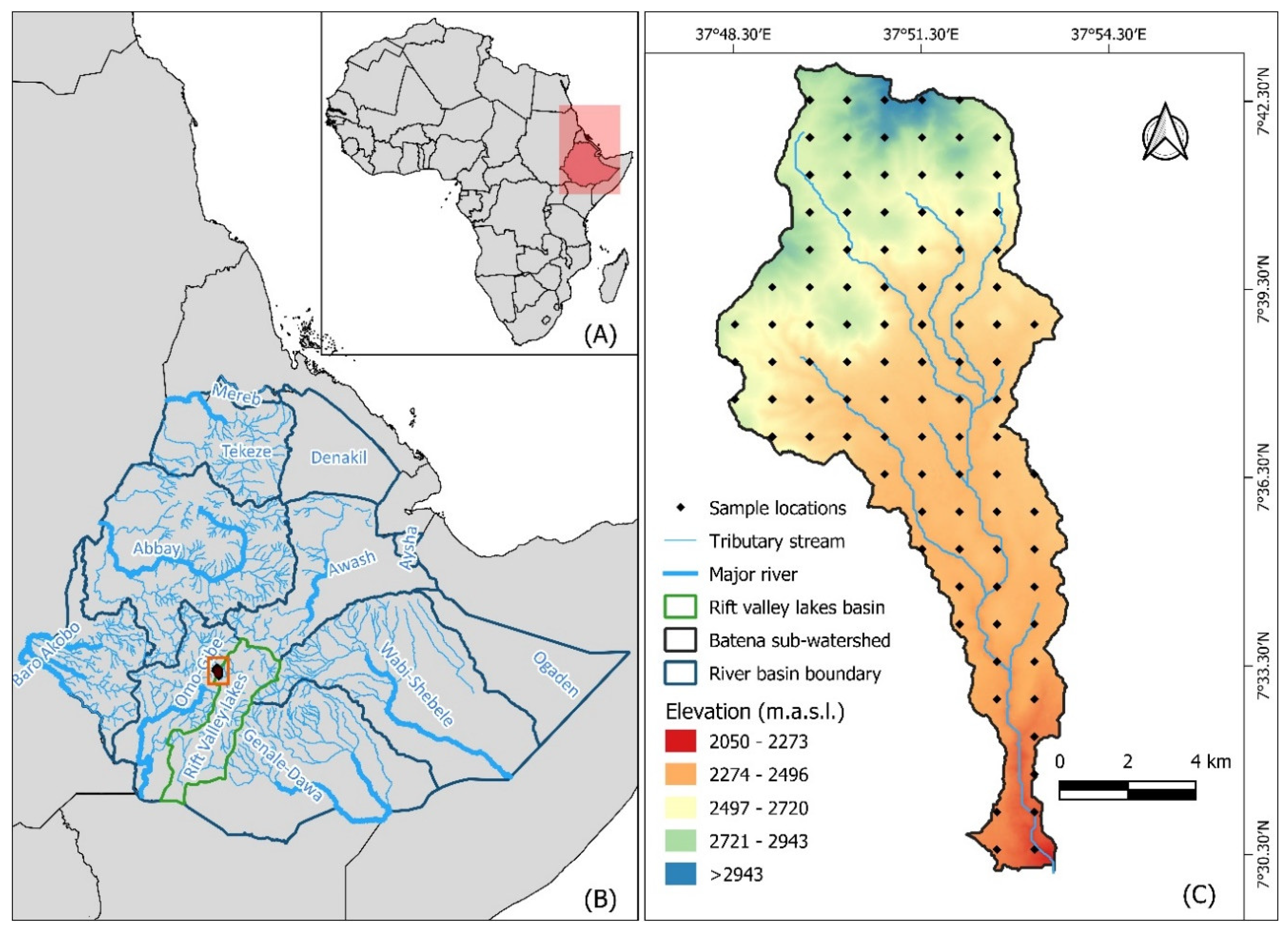
2.1. Study Area
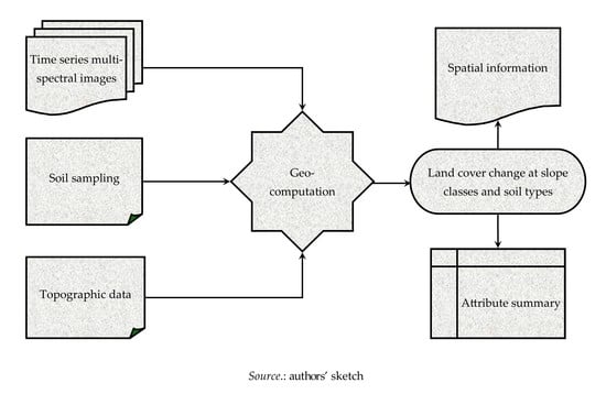
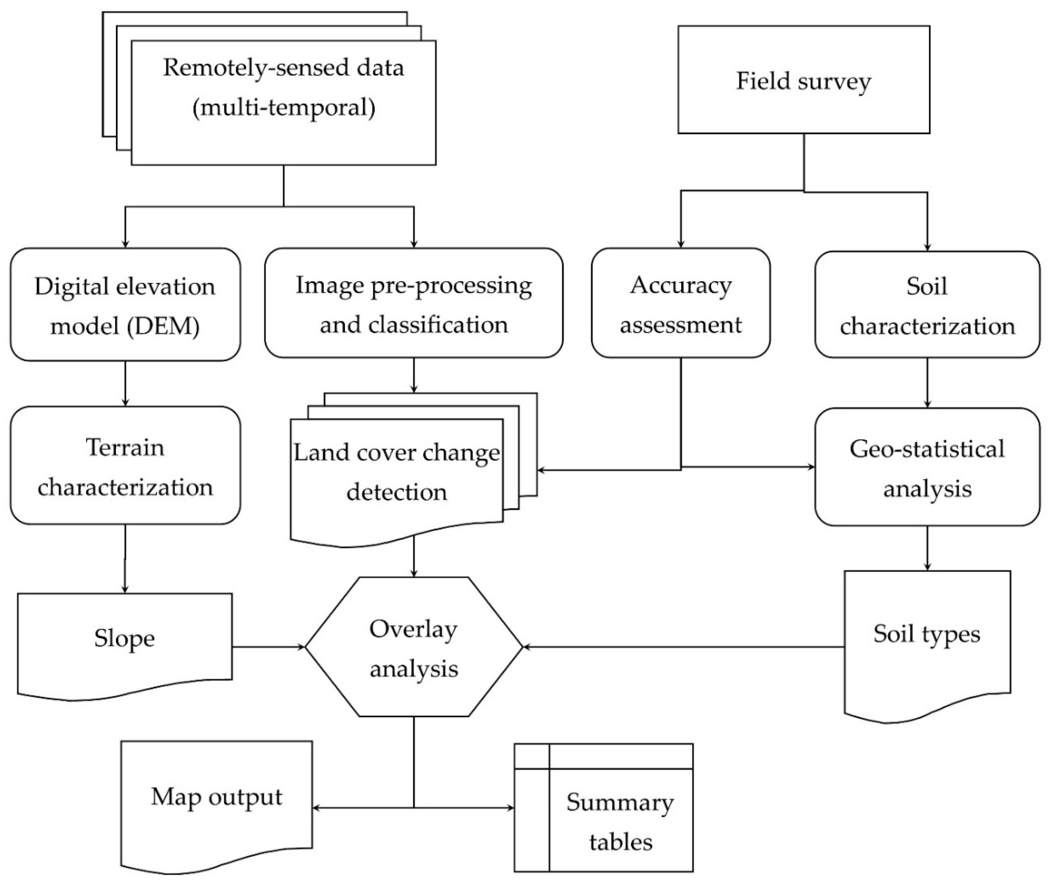
2.2. Methodology
2.2.1. Datasets
2.2.2. Image Processing
2.2.3. Land Cover Change Detection
2.3. Accuracy Assessment
2.4. Soil, Topography, and Land Cover Characterization
2.4.1. Soil Survey and Mapping
2.4.2. Relationship of Soil, Topography, and Land Cover
3. Results and Discussion
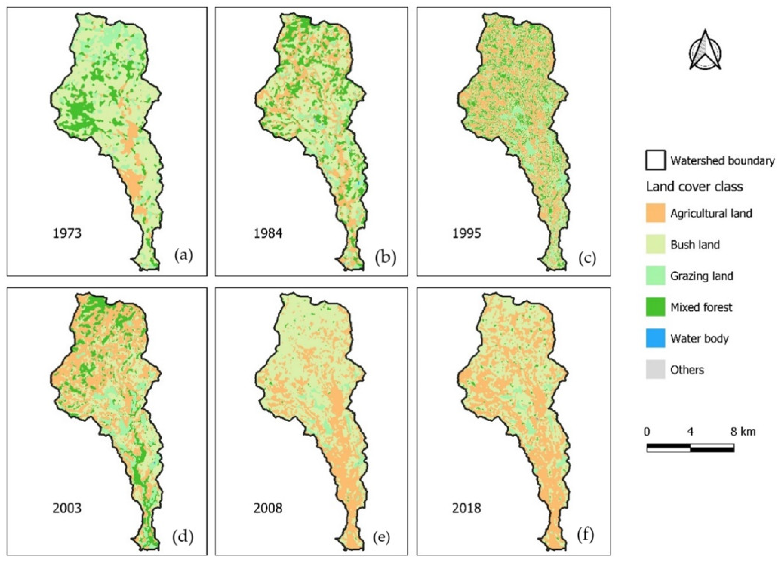
3.1. Land Cover Change
Land Cover Change Intensity
3.2. Relationship of Soil, Topography, and Land Cover
3.2.1. Soil Spatial Analysis, Classification, and Mapping
3.2.2. Terrain Effects on Soil Physicochemical Properties and Land Cover Distribution
3.3. Socioeconomic Impacts of Land Cover Change
4. Conclusions
Supplementary Materials
Author Contributions
Funding
Acknowledgments
Conflicts of Interest
References
- Pitman, A.; de Noblet-Ducoudré, N. Human Effects on Climate through Land-Use Induced Land Cover Change; Future of the World’s Climate/Elsevier: Amsterdam, The Netherlands, 2011; pp. 77–95. [Google Scholar] [CrossRef]
- Oliver, T.H.; Morecroft, M.D. Interactions between climate change and land use change on biodiversity: Attribution problems, risks, and opportunities. Wiley Interdiscip. Rev. Clim. Chang. 2014, 5, 317–335. [Google Scholar] [CrossRef] [Green Version]
- Ayele, G.T.; Tebeje, A.K.; Demissie, S.S.; Belete, M.A.; Jemberrie, M.A.; Teshome, W.M.; Mengistu, D.T.; Teshale, E.Z. Time series land cover mapping and change detection analysis using geographic information system and remote sensing, Northern Ethiopia. Air Soil Water Res. 2018, 11. [Google Scholar] [CrossRef] [Green Version]
- Sahana, M.; Hong, H.Y.; Sajjad, H. Analyzing urban spatial patterns and trend of urban growth using urban sprawl matrix: A study on Kolkata urban agglomeration, India. Sci. Total Environ. 2018, 629, 1557–1566. [Google Scholar] [CrossRef]
- Houet, T.; Loveland, T.R.; Hubert-Moy, L.; Gaucherel, C.; Napton, D.; Barnes, C.A.; Sayler, K. Exploring subtle land use and land cover changes: A framework for future landscape studies. Landsc. Ecol. 2010, 25, 249–266. [Google Scholar] [CrossRef] [Green Version]
- Rechkemmer, A.; von Falkenhayn, L. The human Dimensions of Global Environmental Change: Ecosystem Services, Resilience, and Governance. Erca: From the Human Dimensions of Global Environmental Change to the Observation of the Earth from Space. EPJ Web Conf. 2009, 8, 3–17. [Google Scholar] [CrossRef] [Green Version]
- Ayele, G.T.; Teshale, E.Z.; Yu, B.F.; Rutherfurd, I.D.; Jeong, J. Streamflow and sediment yield prediction for watershed prioritization in the upper blue nile river basin, ethiopia. Water 2017, 9, 782. [Google Scholar] [CrossRef] [Green Version]
- Getachew, H.E.; Melesse, A.M. The impact of land use change on the hydrology of the Angereb watershed, Ethiopia. Int. J. Water Sci. 2012, 1. [Google Scholar] [CrossRef]
- Mango, L.M.; Melesse, A.M.; Mc Clain, M.E.; Gann, D.; Setegn, S.G. Land use and climate change impacts on the hydrology of the upper Mara River Basin, Kenya: Results of a modeling study to support better resource management. Hydrol. Earth Syst. Sci. 2011, 15, 2245–2258. [Google Scholar] [CrossRef] [Green Version]
- Mango, L.M.; Melesse, A.M.; McClain, M.E.; Gann, D.; Setegn, S.G. Hydro-meteorology and water budget of the Mara River Basin under land use change scenarios. In Nile River Basin; Springer: Dordrecht, The Netherlands, 2011; pp. 39–68. [Google Scholar]
- Mohammed, H.; Alamirew, A.; Assen, M.; Melesse, A. Spatiotemporal Mapping of Land Cover in Lake Hardibo Drainage Basin, Northeast Ethiopia: 1957–Water Conservation: Practices, Challenges and Future Implications; Nova Publishers: New York, NY, USA, 2013. [Google Scholar]
- Wondie, M.; Schneider, W.; Melesse, A.M.; Teketay, D. Spatial and temporal land cover changes in the simen mountains national park, a world heritage site in northwestern ethiopia. Remote Sens. 2011, 3, 752–766. [Google Scholar] [CrossRef] [Green Version]
- Hurni, H.; Abate, S.; Bantider, A.; Debele, B.; Ludi, E.; Portner, B.; Yitaferu, B.; Zeleke, G. Land Degradation and Sustainable Land Management in the Highlands of Ethiopia. 2010, pp. 187–207. Available online: https://boris.unibe.ch/5959/1/Hurni_Land%20degradation.pdf (accessed on 4 May 2022).
- Elias, E.; Seifu, W.; Tesfaye, B.; Girmay, W. Impact of land use/cover changes on lake ecosystem of Ethiopia central rift valley. Cogent Food Agric. 2019, 5, 1595876. [Google Scholar] [CrossRef]
- Verburg, P.H.; Crossman, N.; Ellis, E.C.; Heinimann, A.; Hostert, P.; Mertz, O.; Nagendra, H.; Sikor, T.; Erb, K.H.; Golubiewski, N.; et al. Land system science and sustainable development of the earth system: A global land project perspective. Anthropocene 2015, 12, 29–41. [Google Scholar] [CrossRef] [Green Version]
- Gebreslassie, H. Land use-land cover dynamics of Huluka watershed, Central Rift Valley, Ethiopia. Int. Soil Water Conserv. Res. 2014, 2, 25–33. [Google Scholar] [CrossRef] [Green Version]
- Mengistu, K.T. Watershed Hydrological Responses to Changes in Land Use and Land Cover, and Management Practices at Hare Watershed, Ethiopia. Ph.D. Thesis, der Universität Siegen, Sigen, Germany, 2009. [Google Scholar]
- Ariti, A.T.; van Vliet, J.; Verburg, P.H. Land-use and land-cover changes in the Central Rift Valley of Ethiopia: Assessment of perception and adaptation of stakeholders. Appl. Geogr. 2015, 65, 28–37. [Google Scholar] [CrossRef]
- Asres, R.S.; Tilahun, S.A.; Ayele, G.T.; Melesse, A.M. Analyses of Land Use/Land Cover Change Dynamics in the Upland Watersheds of Upper Blue Nile Basin. In Landscape Dynamics, Soils and Hydrological Processes in Varied Climates; Springer: Cham, Switzerland, 2016; pp. 73–91. [Google Scholar]
- Betru, T.; Tolera, M.; Sahle, K.; Kassa, H. Trends and drivers of land use/land cover change in Western Ethiopia. Appl. Geogr. 2019, 104, 83–93. [Google Scholar] [CrossRef]
- Etefa, G.; Frankl, A.; Lanckriet, S.; Biadgilgn, D.; Gebreyohannes, Z.; Amanuel, Z.; Poesen, J.; Nyssen, J. Changes in land use/cover mapped over 80 years in the Highlands of Northern Ethiopia. J. Geogr. Sci. 2018, 28, 1538–1563. [Google Scholar] [CrossRef] [Green Version]
- Moges, D.M.; Bhat, H.G. An insight into land use and land cover changes and their impacts in Rib watershed, north-western highland Ethiopia. Land Degrad. Dev. 2018, 29, 3317–3330. [Google Scholar] [CrossRef]
- Dodgson, N.A. Image Resampling; University of Cambridge, Computer Laboratory: Cambridge, UK, 1992. [Google Scholar]
- Ceddia, M.B.; Vieira, S.R.; Villela, A.L.O.; Mota, L.D.S.; Anjos, L.H.C.D.; Carvalho, D.F.D. Topography and spatial variability of soil physical properties. Sci. Agric. 2009, 66, 338–352. [Google Scholar] [CrossRef] [Green Version]
- O’Geen, A. Soil water dynamics. Nat. Educ. Knowl. 2012, 3, 12. [Google Scholar]
- Luo, Y.; Yang, S.; Zhao, C.; Liu, X.; Liu, C.; Wu, L.; Zhao, H.; Zhang, Y. The effect of environmental factors on spatial variability in land use change in the high-sediment region of China’s Loess Plateau. J. Geogr. Sci. 2014, 24, 802–814. [Google Scholar] [CrossRef] [Green Version]
- Rawat, J.S.; Kumar, M. Monitoring land use/cover change using remote sensing and GIS techniques: A case study of Hawalbagh block, district Almora, Uttarakhand, India. Egypt. J. Remote Sens. Space Sci. 2015, 18, 77–84. [Google Scholar] [CrossRef] [Green Version]
- Otukei, J.R.; Blaschke, T. Land cover change assessment using decision trees, support vector machines and maximum likelihood classification algorithms. Int. J. Appl. Earth Obs. Geoinf. 2010, 12, S27–S31. [Google Scholar] [CrossRef]
- Li, G.; Lu, D.; Moran, E.; Sant’Anna, S.J. Comparative analysis of classification algorithms and multiple sensor data for land use/land cover classification in the Brazilian Amazon. J. Appl. Remote Sens. 2012, 6, 061706. [Google Scholar] [CrossRef]
- Blaschke, T. Object based image analysis for remote sensing. ISPRS J. Photogramm. Remote Sens. 2010, 65, 2–16. [Google Scholar] [CrossRef] [Green Version]
- Suleiman, Y.; Saidu, S.; Abdulrazaq, S.; Hassan, A.; Abubakar, A. The dynamics of land use land cover change: Using geospatial techniques to promote sustainable urban development in Ilorin Metropolis, Nigeria. Asian Rev. Environ. Earth Sci. 2014, 1, 8–15. [Google Scholar]
- Xu, W.X.; Gu, S.; Zhao, X.Q.; Xiao, J.S.; Tang, Y.H.; Fang, J.Y.; Zhang, J.; Jiang, S. High positive correlation between soil temperature and NDVI from 1982 to 2006 in alpine meadow of the Three-River Source Region on the Qinghai-Tibetan Plateau. Int. J. Appl. Earth Obs. Geoinf. 2011, 13, 528–535. [Google Scholar] [CrossRef]
- Sexton, J.O.; Urban, D.L.; Donohue, M.J.; Song, C.H. Long-term land cover dynamics by multi-temporal classification across the Landsat-5 record. Remote Sens. Environ. 2013, 128, 246–258. [Google Scholar] [CrossRef]
- Ahmad, A.; Quegan, S. Analysis of Maximum Likelihood Classification Technique on Landsat 5 TM Satellite Data of Tropical Land Covers. In Proceedings of the 2012 IEEE International Conference on Control, System, Computing and Engineering (ICCSCE 2012), Penang, Malaysia, 23–25 November 2012; pp. 280–285. [Google Scholar]
- Li, M.; Zang, S.Y.; Zhang, B.; Li, S.S.; Wu, C.S. A Review of Remote Sensing Image Classification Techniques: The Role of Spatio-contextual Information. Eur. J. Remote Sens. 2014, 47, 389–411. [Google Scholar] [CrossRef]
- Singh, A. Review article digital change detection techniques using remotely-sensed data. Int. J. Remote Sens. 1989, 10, 989–1003. [Google Scholar] [CrossRef] [Green Version]
- Benito-Calvo, A.; De la Torre, I.; Mora, R.; Tibebu, D.; Morán, N.; Martínez-Moreno, J. Geoarchaeological Potential of the Western Bank of the Bilate River (Ethiopia); Analele Universitatii din Oradea XVIISeria Geographie: Madrid, Spain, 2007; pp. 99–104. [Google Scholar]
- Roy, D.P.; Ju, J.C.; Kline, K.; Scaramuzza, P.L.; Kovalskyy, V.; Hansen, M.; Loveland, T.R.; Vermote, E.; Zhang, C.S. Web-enabled Landsat Data (WELD): Landsat ETM plus composited mosaics of the conterminous United States. Remote Sens. Environ. 2010, 114, 35–49. [Google Scholar] [CrossRef]
- Crippen, R.E. A simple spatial filtering routine for the cosmetic removal of scan-line noise from Landsat TM P-tape imagery. Photogramm. Eng. Remote Sens. 1989, 55, 327–331. [Google Scholar]
- Richards John, A.; Xiuping, J. Remote Sensing Digital Image Analysis: An Introduction; Springer: Berlin, Germany, 1999. [Google Scholar]
- Ju, J.C.; Roy, D.P.; Vermote, E.; Masek, J.; Kovalskyy, V. Continental-scale validation of MODIS-based and LEDAPS Landsat ETM plus atmospheric correction methods. Remote Sens. Environ. 2012, 122, 175–184. [Google Scholar] [CrossRef] [Green Version]
- Bakker, W.H.; Grabmaier, K.; Hunmeman, G.; Van Der Meer, F.; Prakash, A.; Tempfli, K.; Gieske, A.; Hecker, C.; Janseen, L.; Parodi, G. Principles of Remote Sensing, An Introductory Textbook; The International Institute for Geo-Informational Science and Earth Observation (ITC): Enschede, The Netherlands, 2004. [Google Scholar]
- Serra, P.; Pons, X.; Sauri, D. Post-classification change detection with data from different sensors: Some accuracy considerations. Int. J. Remote Sens. 2003, 24, 4975–4976. [Google Scholar] [CrossRef]
- Sabins, F.F., Jr.; Ellis, J.M. Remote Sensing: Principles, Interpretation, and Applications; Waveland Press: Long Grove, IL, USA, 2020. [Google Scholar]
- Mesfin, D.; Simane, B.; Belay, A.; Recha, J.W.; Taddese, H. Woodland cover change in the Central Rift Valley of Ethiopia. Forests 2020, 11, 916. [Google Scholar] [CrossRef]
- Lu, D.; Mausel, P.; Batistella, M.; Moran, E. Land-cover binary change detection methods for use in the moist tropical region of the Amazon: A comparative study. Int. J. Remote Sens. 2005, 26, 101–114. [Google Scholar] [CrossRef]
- World Reference Base for Soil Resources. A Framework for International Classification, Correlation and Communication; World Soil Resources Reports; Resources: Rome, Italy, 2006; Volume 103. [Google Scholar]
- Sachez-Reyes, U.J.; Nino-Maldonado, S.; Barrientos-Lozano, L.; Trevino-Carreon, J. Assessment of Land Use-Cover Changes and Successional Stages of Vegetation in the Natural Protected Area Altas Cumbres, Northeastern Mexico, Using Landsat Satellite Imagery. Remote Sens. 2017, 9, 712. [Google Scholar] [CrossRef] [Green Version]
- Mas, J.-F. Monitoring land-cover changes: A comparison of change detection techniques. Int. J. Remote Sens. 1999, 20, 139–152. [Google Scholar] [CrossRef]
- Congalton, R.G.; Green, K. Assessing the Accuracy of Remotely Sensed Data: Principles and Practices; CRC Press: Boca Raton, FL, USA, 2002. [Google Scholar]
- Anderson, J.R. A Land Use and Land Cover Classification System for Use with Remote Sensor Data; US Government Printing Office: Washington, WA, USA, 1976; Volume 964.
- Congalton, R.G. Accuracy assessment: A critical component of land cover mapping. Gap Anal. 1996. [Google Scholar] [CrossRef] [Green Version]
- United States Department of Agriculture, Soil Taxonomy. A Basic System of Soil Classification for Making and Interpreting Soil Surveys; USDA: Pittsburgh, PA, USA, 1999; Volume 436, pp. 96–105.
- Webster, R. Is soil variation random? Geoderma 2000, 97, 149–163. [Google Scholar] [CrossRef]
- Isaaks, E.; Srivastava, R. Applied Geostatistics. An Introduction to Applied Geoestatistics; Oxford University Press: Oxford, UK, 1989. [Google Scholar]
- Ayele, G.T.; Demissie, S.S.; Jemberrie, M.A.; Jeong, J.; Hamilton, D.P. Terrain Effects on the Spatial Variability of Soil Physical and Chemical Properties. Soil Syst. 2019, 4, 1. [Google Scholar] [CrossRef] [Green Version]
- Morgan, C.J. Theoretical and Practical Aspects of Variography: In Particular, Estimation and Modelling of Semi-Variograms over Areas of Limited and Clustered or Widely Spaced Data in a Two-Dimensional South African Gold Mining Context. Ph.D. Thesis, University of the Witwatersrand, Johannesburg, South Africa, 2011. [Google Scholar]
- Mcbratney, A.B.; Webster, R. Choosing Functions for Semi-Variograms of Soil Properties and Fitting Them to Sampling Estimates. J. Soil Sci. 1986, 37, 617–639. [Google Scholar] [CrossRef]
- Warrick, A. Spatial variability of soil physical properties in the field. Appl. Soil Phys. 1980, 319–344. Available online: https://www.researchgate.net/publication/300071023_Spatial_Variability_of_Soil_Physical_Properties_in_a_Cultivated_Field (accessed on 4 May 2022).
- Assefa, F.; Elias, E.; Soromessa, T.; Ayele, G.T. Effect of changes in land-use management practices on soil physicochemical properties in Kabe Watershed, Ethiopia. Air Soil Water Res. 2020, 13. [Google Scholar] [CrossRef]
- Kumar, A.; Padbhushan, R.; Singh, Y.K.; Kohli, A.; Ghosh, M. Soil organic carbon under various land uses in alfisols of Eastern India. Indian J. Agril. Sci. 2021, 91, 975–979. [Google Scholar]
- Coburn, T.C. Geostatistics for Natural Resources Evaluation; Taylor & Francis: Milton Park, UK, 2000. [Google Scholar]
- Girmay, W.; Tesfaye, B.; Seifu, W.; Elias, E. Effect of Land Use/Cover Changes on Ecological Landscapes of the Four Lakes of Central Rift Valley Ethiopia. J. Environ. Earth Sci. 2017, 7, 12. [Google Scholar]
- Muzein, B.S. Remote Sensing & GIS for Land Cover, Land Use Change Detection and Analysis in the Semi-Natural Ecosystems and Agriculture Landscapes of the Central Ethiopian Rift Valley. 2006. Available online: http://www.vinr.ir/sites/default/files/Muzein2006.pdf (accessed on 4 May 2022).
- How Jin Aik, D.; Ismail, M.H.; Muharam, F.M.; Alias, M.A. Evaluating the impacts of land use/land cover changes across topography against land surface temperature in Cameron Highlands. PLoS ONE 2021, 16, e0252111. [Google Scholar] [CrossRef] [PubMed]
- Mengistu, D.K.; Woldetsadik, M. Detection and analysis of land-use and land-cover changes in the Midwest escarpment of the Ethiopian Rift Valley. J. Land Use Sci. 2012, 7, 239–260. [Google Scholar] [CrossRef]
- Spaargaren, O.C.; Deckers, J. The world reference base for soil resources. In Soils of Tropical Forest Ecosystems; Springer: Berlin, Germany, 1998; pp. 21–28. [Google Scholar]
- de Valenca, A.W.; Vanek, S.J.; Meza, K.; Ccanto, R.; Olivera, E.; Scurrah, M.; Lantinga, E.A.; Fonte, S.J. Land use as a driver of soil fertility and biodiversity across an agricultural landscape in the Central Peruvian Andes. Ecol. Appl. 2017, 27, 1138–1154. [Google Scholar] [CrossRef]
- Jemberie, M.A.; Awass, A.A.; Melesse, A.M.; Ayele, G.T.; Demissie, S.S. Seasonal Rainfall-Runoff Variability Analysis, Lake Tana Sub-Basin, Upper Blue Nile Basin, Ethiopia. In Landscape Dynamics, Soils and Hydrological Processes in Varied Climates; Springer: Cham, Switzerland, 2016. [Google Scholar] [CrossRef]
- Seka, A.M.; Awass, A.A.; Melesse, A.M.; Ayele, G.T.; Demissie, S.S. Evaluation of the Effects of Water Harvesting on Downstream Water Availability Using SWAT. In Landscape Dynamics, Soils and Hydrological Processes in Varied Climates; Springer: Cham, Switzerland, 2016. [Google Scholar] [CrossRef]
- Conforti, M.; Buttafuoco, G. Assessing space–time variations of denudation processes and related soil loss from 1955 to 2016 in southern Italy (Calabria region). Environ. Earth Sci. 2017, 76, 457. [Google Scholar] [CrossRef]
- Balba, A.M. Management of Problem Soils in Arid Ecosystems; CRC Press: Boca Raton, FL, USA, 2018. [Google Scholar]
- Abate, N.; Kibret, K. Effects of land use, soil depth and topography on soil physicochemical properties along the toposequence at the Wadla Delanta Massif, Northcentral Highlands of Ethiopia. Environ. Pollut 2016, 5, 57–71. [Google Scholar] [CrossRef] [Green Version]
- Griffiths, R.P.; Madritch, M.D.; Swanson, A.K. The effects of topography on forest soil characteristics in the Oregon Cascade Mountains (USA): Implications for the effects of climate change on soil properties. For. Ecol. Manag. 2009, 257, 1–7. [Google Scholar] [CrossRef]
- Hu, H.; Ma, H.; Wang, Y.; Xu, H. Influence of land use types to nutrients, organic carbon and organic nitrogen of soil. Soill Water Conserv. China 2010, 11, 40–42. [Google Scholar]
- Gashaw, T.; Tulu, T.; Argaw, M.; Worqlul, A.W. Evaluation and prediction of land use/land cover changes in the Andassa watershed, Blue Nile Basin, Ethiopia. Environ. Syst. Res. 2017, 6, 17. [Google Scholar] [CrossRef] [Green Version]
- Gebru, B.M.; Lee, W.K.; Khamzina, A.; Lee, S.G.; Negash, E. Hydrological Response of Dry Afromontane Forest to Changes in Land Use and Land Cover in Northern Ethiopia. Remote Sens. 2019, 11, 1905. [Google Scholar] [CrossRef] [Green Version]
- Miheretu, B.A.; Yimer, A.A. Determinants of farmers’ adoption of land management practices in Gelana sub-watershed of Northern highlands of Ethiopia. Ecol. Processes 2017, 6, 19. [Google Scholar] [CrossRef] [Green Version]
- Wubie, M.A.; Assen, M.; Nicolau, M.D. Patterns, causes and consequences of land use/cover dynamics in the Gumara watershed of lake Tana basin, Northwestern Ethiopia. Environ. Syst. Res. 2016, 5, 8. [Google Scholar] [CrossRef] [Green Version]
- Li, S.C.; Bing, Z.L.; Jin, G. Spatially Explicit Mapping of Soil Conservation Service in Monetary Units Due to Land Use/Cover Change for the Three Gorges Reservoir Area, China. Remote Sens. 2019, 11, 468. [Google Scholar] [CrossRef] [Green Version]
- Wolka, K.; Tadesse, H.; Garedew, E.; Yimer, F. Soil erosion risk assessment in the Chaleleka wetland watershed, Central Rift Valley of Ethiopia. Environ. Syst. Res. 2015, 4, 5. [Google Scholar] [CrossRef] [Green Version]
- Wijitkosum, S. Impacts of land use changes on soil erosion in Pa Deng sub-district, adjacent area of Kaeng Krachan National Park, Thailand. Soil Water Res. 2012, 7, 10–17. [Google Scholar] [CrossRef] [Green Version]
- Valentin, C.; Agus, F.; Alamban, R.; Boosaner, A.; Bricquet, J.-P.; Chaplot, V.; De Guzman, T.; De Rouw, A.; Janeau, J.-L.; Orange, D. Runoff and sediment losses from 27 upland catchments in Southeast Asia: Impact of rapid land use changes and conservation practices. Agric. Ecosyst. Environ. 2008, 128, 225–238. [Google Scholar] [CrossRef]
- Mekonnen, Z.; Berie, H.T.; Woldeamanuel, T.; Asfaw, Z.; Kassa, H. Land use and land cover changes and the link to land degradation in Arsi Negele district, Central Rift Valley, Ethiopia. Remote Sens. Appl. Soc. Environ. 2018, 12, 1–9. [Google Scholar] [CrossRef]


| Sensor Type | Date of Acquisition | Path | Row | Spatial Resolution (m) | Temporal Resolution (Days) |
|---|---|---|---|---|---|
| MSS | 31 January 1973 | 181 | 55 | 60 | 18 |
| TM | 22 November 1984 | 169 | 55 | 30 | 16 |
| TM | 21 January 1995 | 169 | 55 | 30 | 16 |
| ETM+ | 24 November 2003 | 169 | 55 | 30 | 16 |
| ETM+ | 27 November 2008 | 169 | 55 | 30 | 16 |
| OLI | 20 November 2018 | 169 | 55 | 30 | 16 |
| Years | ||||||||||||
|---|---|---|---|---|---|---|---|---|---|---|---|---|
| LC Type | 1973 | 1984 | 1995 | 2003 | 2008 | 2018 | ||||||
| km2 | % | km2 | % | km2 | % | km2 | % | km2 | % | km2 | % | |
| Agriculture | 11.7 | 10.0 | 31.0 | 26.6 | 46.0 | 39.5 | 48.3 | 41.4 | 50.2 | 43.0 | 56.5 | 48.4 |
| Bushland | 69.7 | 59.7 | 51.4 | 44.2 | 43.6 | 37.4 | 34.9 | 29.9 | 54.1 | 46.4 | 52.8 | 45.2 |
| Grazing land | 15.8 | 13.5 | 10.2 | 8.8 | 8.6 | 7.3 | 12.2 | 10.5 | 5.8 | 5.0 | 4.8 | 4.1 |
| Mixed forest | 19.5 | 16.7 | 23.9 | 20.5 | 18.4 | 15.8 | 21.2 | 18.2 | 6.6 | 5.6 | 2.7 | 2.3 |
| Total area | 116.7 | 116.7 | 116.7 | 116.7 | 116.7 | 116.7 | ||||||
| Overall acc. | 95.1 | 99.2 | 95.2 | 96.2 | 98.2 | 90.4 | ||||||
| 92.3 | 98.4 | 93.3 | 97.8 | 97.1 | 93.2 | |||||||
| Initial State | Final State (2018) | ||||||
|---|---|---|---|---|---|---|---|
| AL | BL | GL | MF | RT | Gain | ||
| 1973 | AL | 8.3 | 31.4 | 8.0 | 8.8 | 56.5 | 48.2 |
| BL | 2.6 | 33.3 | 6.8 | 9.9 | 52.8 | 19.4 | |
| GL | 0.6 | 3.4 | 0.6 | 0.1 | 4.8 | 4.1 | |
| MF | 0.1 | 1.5 | 0.3 | 0.7 | 2.7 | 1.9 | |
| CT | 11.7 | 69.7 | 15.8 | 19.5 | 116.7 | ||
| CC | 3.4 | 36.3 | 15.1 | 18.8 | |||
| ID | 44.8 | −16.9 | −11.0 | −16.9 | |||
| 1984 | AL | 21.0 | 27.2 | 4.3 | 3.9 | 56.5 | 35.4 |
| BL | 9.2 | 22.9 | 2.0 | 18.6 | 52.8 | 29.9 | |
| GL | 0.4 | 0.4 | 3.9 | 0.03 | 4.8 | 0.9 | |
| MF | 0.3 | 1.0 | 0.02 | 1.4 | 2.7 | 1.3 | |
| CT | 31.0 | 51.4 | 10.2 | 23.9 | 116.7 | ||
| CC | 9.9 | 28.5 | 6.3 | 22.5 | |||
| ID | 25.5 | 1.3 | −5.4 | −21.2 | |||
| 1995 | AL | 34.2 | 17.2 | 3.1 | 2.0 | 56.5 | 22.2 |
| BL | 11.5 | 24.1 | 2.1 | 15.1 | 52.8 | 28.7 | |
| GL | 0.2 | 1.1 | 3.4 | 0.02 | 4.8 | 1.4 | |
| MF | 0.1 | 1.2 | 0.04 | 1.3 | 2.7 | 1.3 | |
| CT | 46.0 | 43.6 | 8.6 | 18.4 | 116.7 | ||
| CC | 11.8 | 19.6 | 5.2 | 17.1 | |||
| ID | 10.4 | 9.1 | −3.8 | −15.8 | |||
| 2003 | AL | 29.7 | 11.9 | 5.6 | 9.3 | 56.5 | 26.8 |
| BL | 17.8 | 21.4 | 2.5 | 11.1 | 52.8 | 31.4 | |
| GL | 0.4 | 0.2 | 4.1 | 0.1 | 4.8 | 0.7 | |
| MF | 0.45 | 1.40 | 0.03 | 0.77 | 2.7 | 1.9 | |
| CT | 48.3 | 34.9 | 12.2 | 21.2 | 116.7 | ||
| CC | 18.6 | 13.6 | 8.1 | 20.4 | |||
| ID | 8.2 | 17.8 | −7.5 | −18.5 | |||
| 2008 | AL | 46.0 | 7.3 | 0.6 | 2.6 | 56.5 | 10.5 |
| BL | 3.3 | 43.9 | 2.4 | 3.2 | 52.8 | 8.9 | |
| GL | 0.9 | 1.6 | 2.3 | 0.0 | 4.8 | 2.5 | |
| MF | 1.3 | 0.5 | 0.8 | 2.7 | 1.8 | ||
| CT | 50.2 | 54.1 | 5.8 | 6.6 | 116.7 | ||
| CC | 4.2 | 10.2 | 3.5 | 5.8 | |||
| ID | 6.3 | −1.3 | −1.0 | −3.9 | |||
Publisher’s Note: MDPI stays neutral with regard to jurisdictional claims in published maps and institutional affiliations. |
© 2022 by the authors. Licensee MDPI, Basel, Switzerland. This article is an open access article distributed under the terms and conditions of the Creative Commons Attribution (CC BY) license (https://creativecommons.org/licenses/by/4.0/).
Share and Cite
Ayele, G.T.; Seka, A.M.; Taddese, H.; Jemberrie, M.A.; Ndehedehe, C.E.; Demissie, S.S.; Awange, J.L.; Jeong, J.; Hamilton, D.P.; Melesse, A.M. Relationship of Attributes of Soil and Topography with Land Cover Change in the Rift Valley Basin of Ethiopia. Remote Sens. 2022, 14, 3257. https://doi.org/10.3390/rs14143257
Ayele GT, Seka AM, Taddese H, Jemberrie MA, Ndehedehe CE, Demissie SS, Awange JL, Jeong J, Hamilton DP, Melesse AM. Relationship of Attributes of Soil and Topography with Land Cover Change in the Rift Valley Basin of Ethiopia. Remote Sensing. 2022; 14(14):3257. https://doi.org/10.3390/rs14143257
Chicago/Turabian StyleAyele, Gebiaw T., Ayalkibet M. Seka, Habitamu Taddese, Mengistu A. Jemberrie, Christopher E. Ndehedehe, Solomon S. Demissie, Joseph L. Awange, Jaehak Jeong, David P. Hamilton, and Assefa M. Melesse. 2022. "Relationship of Attributes of Soil and Topography with Land Cover Change in the Rift Valley Basin of Ethiopia" Remote Sensing 14, no. 14: 3257. https://doi.org/10.3390/rs14143257
APA StyleAyele, G. T., Seka, A. M., Taddese, H., Jemberrie, M. A., Ndehedehe, C. E., Demissie, S. S., Awange, J. L., Jeong, J., Hamilton, D. P., & Melesse, A. M. (2022). Relationship of Attributes of Soil and Topography with Land Cover Change in the Rift Valley Basin of Ethiopia. Remote Sensing, 14(14), 3257. https://doi.org/10.3390/rs14143257