A Discriminative Spectral-Spatial-Semantic Feature Network Based on Shuffle and Frequency Attention Mechanisms for Hyperspectral Image Classification

Abstract

Due to end-to-end optimization characteristics and fine generalization ability, convolutional neural networks have been widely applied to hyperspectral image (HSI) classification, playing an irreplaceable role. However, previous studies struggle with two major challenges: (1) HSI contains complex topographic features, the number of labeled samples in different categories is unbalanced, resulting in poor classification for categories with few labeled samples; (2) With the deepening of neural network models, it is difficult to extract more discriminative spectral-spatial features. To address the issues mentioned above, we propose a discriminative spectral-spatial-semantic feature network based on shuffle and frequency attention mechanisms for HSI classification. There are four main parts of our approach: spectral-spatial shuffle attention module (SSAM), context-aware high-level spectral-spatial feature extraction module (CHSFEM), spectral-spatial frequency attention module (SFAM), and cross-connected semantic feature extraction module (CSFEM). First, to fully excavate the category attribute information, SSAM based on a “Deconstruction-Reconstruction” structure is designed, solving the problem of poor classification performance caused by an unbalanced number of label samples. Considering that deep spectral-spatial features are difficult to extract, CHSFEM and SFAM are constructed. The former is based on the “Horizontal-Vertical” structure to capture context-aware high-level multiscale features. The latter introduces multiple frequency components to compress channels to obtain more multifarious features. Finally, towards suppressing noisy boundaries efficiently and capturing abundant semantic information, CSFEM is devised. Numerous experiments are implemented on four public datasets: the evaluation indexes of OA, AA and Kappa on four datasets all exceed 99%, demonstrating that our method can achieve satisfactory performance and is superior to other contrasting methods.

1. Introduction

A hyperspectral image (HSI) can be captured by hyperspectral remote sensing sensors, which contain abundant spatial and spectral information, covering a wide range of wavelengths. HSI classification aims to assign a pinpoint land-cover label to each hyper-spectral pixel, which has been widely applied in environmental monitoring [1], mineral exploitation [2], object detection [3], defense and security [4], etc.

Although remarkable progress has been achieved, HSI classification still struggles with great challenges, which are described as follows: (1) Spectral variability. The spectral information of HSI is influenced by many external factors, such as atmospheric effects, natural spectrum, and incident illumination [5,6,7], which result in difficulty in identifying a given category due to the high intraclass spectral variability. (2) Spatial variability. The spatial distributions of disparate objects in HSI are complicated, and the ground feature regions contain mixed pixels [8]. There is a phenomenon where different ground targets include the same spectral information and the same ground targets contain different spectral information [9]. (3) The lack of labeled samples. Labeling HSI samples is very inconvenient and time-consuming. Meanwhile, the amount of labeled data is too small, which brings about the Hughes phenomenon [10], meaning that the classification accuracy severely decreases with increasing dimensionality [11]. Therefore, scholars pay more attention to settling the above problems [12,13,14,15,16,17].

In the initial phase, traditional machine learning methods have mainly been com-posed of two steps: feature extraction and classifier training [18]. First, traditional feature extraction methods, including linear discriminant analysis (LDA) [19], minimum noise fraction (MNF) [20], spectral angle mapper (SAM) [21], and principal component analysis (PCA) [22] are utilized to capture spectral features. Then, these obtained spectral features are sent into the classifiers, which include support vector machine (SVM) [23], multinomial logistic regression (MLR) [24], k-nearest neighbor (KNN) [25], random forest (RF) [26], etc. However, these traditional classification methods based on spectral features do not take full advantage of the spatial information of HSI. Therefore, traditional HSI classification methods based on spectral-spatial features are proposed. Some successful statistical methods are used to extract spectral and spatial data from HSI, such as the Markov random field (MRF) [27] and the conditional random field (CRF) [28]. Paul et al. proposed a particle swarm optimization-based unsupervised dimensionality reduction method for HSI classification, where spectral and spatial information is utilized to select informative bands [29]. Sparse representation-based classifiers (SRCs) [30], adaptive nonlocal spatial-spectral kernels (ANSSKs) [31], and SVMs with composite kernels (SVMCKs) [32] introduced spatial features into HSI classification to effectively explore the spatial information with spectral features. Yu et al. developed a semisupervised band selection (BS) approach based on dual-constrained low-rank representation BS for HSI classification [33]. Nevertheless, traditional HSI classification methods, whether they are based on spectral information or spectral-spatial information, all rely on handcrafted features with limited represented ability, which results in poor generalization ability.

With the development of computer vision, numerous effective HSI classification methods based on deep learning have been presented. Typical deep learning methods include deep belief networks (DBNs), convolutional neural networks (CNNs), recurrent neural networks (RNNs), and stacked auto-encoders (SAEs). CNNs have the power to extract nonlinear and hierarchical features, which have prompted much attention for remote sensing processing. For example, Hu et al. presented a deep CNN with five 1-D convolutional layers that received pixel vectors as input data, classifying HSI data cubes only in the spectral domain [34]. Mei et al. trained the model by considering the mean and standard deviation per spectral band of the neighboring pixels, the spectrum of the pixel, and the spectral mean of neighboring pixels, introducing several improvements into the CNN1D architecture [35]. However, the input of these classification methods based on 1-D CNN must be flattened into 1-D vectors, resulting in the underutilization of the spatial information.

Recently, deep learning classification methods utilizing spectral and spatial information have been gradually developed to effectively learn discriminative representations and hierarchical features. For instance, Slavkovikj et al. integrated spectral and spatial information into a 1-D kernel by reconstructing the spectral-spatial neighbourhood window [36]. He et al. used covariance matrices to train the 2-D CNN, which encoded the spectral-spatial information of diverse size neighborhoods of 20 principal components and obtained multiscale covariance maps [37]. Lee et al. introduced a context deep CNN to explore local contextual interactions, where 2-D CNN was utilized to capture spectral and spatial separate features [38]. Chen et al. introduced a supervised 2-D CNN and a 3-D CNN for classification; here, the 2-D CNN was composed of three 2-D convolutional layers and the 3-D CNN consisted of three 3-D convolutional layers [39]. Although these HSI classification methods can make use of the spatial context information, the spectral-spatial joint features achieved are separated into two independent parts. Therefore, some spectral-spatial classification methods are proposed to learn the joint spectral-spatial information. To effectively investigate the spectral-spatial information, Xi et al. presented a deep prototypical network with hybrid residual attention [40]. To maximize the exploitation of the global and multiscale information of HIS, Yu et al. presented a dual-channel convolutional network for HSI classification [41]. Zhu et al. constructed a novel deformable CNN-based HSI classification method, where the deformable convolutional sampling locations were introduced to adaptively adjust the HSI spatial context [42]. Rao et al. designed a Siamese CNN with a 3-D adaptive spatial spectrum pyramid pooling layer, whose input was 3D sample pairs of different sizes, regardless of the number of spectral bands [43]. To fully explore the discriminant features, Zhan et al. innovated a three-direction spectral-spatial convolution neural network to improve the accuracy of change detection [44]. To eliminate redundant information and interclass interference, Ge et al. designed an adaptive hash attention and lower triangular network for HSI classification [45]. Although these classification methods can extract deep joint spectral-spatial features, it is still inconvenient for them to focus more on discriminated feature regions and restrain the unnecessary information from plentiful spectral-spatial features.

Inspired by the attention mechanisms of human visual perception, many researchers introduce the attention mechanism into HSI classification to focus on the most valuable information parts. For example, Gao et al. explicitly modeled independencies between channels to adaptively recalibrate channel feature responses by introducing the squeeze-and-excitation network [46]. To solve the problem of large amounts of initial information being lost in CNN pipelines, Lin et al. proposed an attention-aware pseudo-3-D (AP3D) convolutional network for HSI classification [47]. Yang et al. designed an end-to-end residual spectral-spatial attention network to accelerate the training process and avoid overfitting [48]. Hang et al. constructed a spectral attention subnetwork and a spatial attention subnetwork for spectral and spatial features classification [49]. To improve feature processing for HSI classification, Paoletti et al. devised multiple attention-guided capsule networks [50]. Although these classification methods based on the attention mechanisms can achieve good classification accuracy, their attention modules are too simple and only optimize in a spectral or spatial dimension. In addition, due to the simple concatenate operation between spectral and spatial features, it may have lost a large amount of important information and be difficult to capture high-level semantic features.

To solve the aforementioned problems, we propose a discriminative spectral-spatial-semantic feature network based on shuffle and frequency attention mechanisms for HSI classification, where multiple functional modules are constructed based on CNNs. First, we design a spectral-spatial shuffle attention module, which can not only capture local and global spectral and spatial separate features, but also integrate the large short-range correlation between spectral and spatial features, while modeling the large long-range interdependency of spectral and spatial data. With these network units, the category attribute information of HSI can be fully excavated. Second, a context-aware high-level spectral-spatial feature extraction module is constructed to extract the multiscale high-level context features of scale invariance, further enriching category semantic information, and outputting more abstract and robust high-resolution representations. Then, to compress the spectral channels and obtain more manifold spectral-spatial features, we utilize a spectral-spatial frequency attention module, which introduces multiple frequency components and enriches high-level semantic information for classification. Sequentially, we present a cross-connected semantic feature extraction module, which not only extracts the global context of high-level semantic features, but also suppresses noisy boundaries. Finally, dropout and batch normalization (BN) optimization methods are introduced into the proposed method to ameliorate the classification performance.

The main contributions of this work can be summarized as follows:

(1)

To fully excavate the category attribute information of HSI, we design a spectral-spatial shuffle attention module (SSAM). First, SSAM extracts local and global spectral and spatial independent features. Second, SSAM aggregates the large short-range close relationship between spectral and spatial features and updates the large long-range interdependency of spectral and spatial data.

(2)

We construct a context-aware high-level spectral-spatial feature extraction module (CHSFEM) to capture the multiscale high-level spectral-spatial features of scale invariance. The CHSFEM can not only enrich discriminative spectral-spatial multiscale features for limited labeled data, but also maintain high-resolution representations throughout the process and repeatedly fuse multiscale subnet features.

(3)

We utilize a spectral-spatial frequency attention module (SFAM) to adaptively compress the spectral channels and introduce multiple frequency components, which achieves manifold spectral-spatial features and enriches high-level semantic features for classification.

(4)

To obtain the global context semantic features, we develop a cross-connected semantic feature extraction module (CSFEM) between the encoder part and the decoder part. The CSFEM can effectually suppress noisy boundaries. Meanwhile, the spectral-spatial shuffle attention features from the encoder phase can be weighted by the diverse high-level frequency attention features and select shuffle attention features that are more valuable to HSI classification, sequentially contributing to high-level frequency attention features, restoring the boundaries of categories in the decoder phase.

The rest of this article is organized as follows: In Section 2, the proposed methods are introduced in detail. In Section 3, the experiments and results are analyzed and discussed. Finally, in Section 4, we conclude this article and describe our future work.

2. The Proposed Hyperspectral Image Classification Method

This paper proposes a discriminative spectral-spatial-semantic feature network based on shuffle and frequency attention mechanisms for HSI classification (DSFNet). The detailed structure of DSFNet is provided in Figure 1. The DSFNet consists of four main parts: the initial module, the encoder phase, the decoder stage, and the classification module. In proposed DSFNet, 3-D image cube of size $23\times 23\times 10$ is chosen from the raw hyperspectral dataset using PCA as a sample. First, we employ the initial module to capture the general spectral-spatial features of the training samples. Next, the encoder phase is designed to capture more abstract and discriminative joint spectral-spatial features, while learning the large short-range and long-range interdependency of spectral and spatial data. Then, we construct a decoder stage, which can not only obtain the high-level global cross-connected semantic features for classification but also take full advantage of the spectral-spatial shuffle and frequency attention features to suppress the noisy boundaries and restore the boundaries of categories. Finally, to enhance the classification performance, we introduce dropout and BN optimization methods into the DSFNet.

2.1. Encoder and Decoder

2.1.1. Encoder Part

As shown in Figure 1, in the encoder stage, we use different network units to acquire more expressive and heterogeneous joint spectral-spatial features, adequately exploring the category attribute information of HSI. The encoder stage involves three dominant parts: the spectral-spatial shuffle attention module (SSAM), the context-aware high-level spectral-spatial feature extraction module (CHSFEM), and the spectral-spatial frequency attention module (SFAM). First, the general feature maps obtained from the initial module are transmitted to two SSAMs. The SSAM is constructed based on a “Deconstruction-Reconstruction” structure, which can not only extract local and global spectral and spatial features separately but also aggregate the large short-range correlation between spectral and spatial information, further modelling the large long-range interdependency of spectral and spatial data. SSAM can not only capture abundant topographic information but also balance the poor classification problem caused by unbalanced samples. The spectral-spatial shuffle attention features obtained from two SSAMs are considered low-level features. Subsequently, the spectral-spatial shuffle attention features are fed into the CHSFEM. The CHSFEM including three subnets, can extract more nonobjective multiscale spectral-spatial features of scale invariance, where we consider the information achieved as high-level features. Furthermore, the high-level spectral-spatial features are sent to three SAFMs. The SAFM introduces multiple frequency components to compress the spectral channels to acquire diversified spectral-spatial features, which complement the reaped high-level features. CHSFEM and SFAM can solve the problem that it is difficult to extract more discriminative spectral-spatial features the deepening of neural network models.

2.1.2. Decoder Part

As expressed in Figure 1, in the decoder stage, several functional modules are employed to output high-level cross-connected spectral-spatial-semantic features for classification. The decoder stage is composed of four CSFEMs. On the one hand, the CSFEM captures global context cross-connected spectral-spatial-semantic features via global average pooling and global max pooling operations for the classification task. On the other hand, the CSFEM can take full advantage of the spectral-spatial shuffle attention features to guide high-level spectral-spatial frequency attention features to suppress the noisy boundaries and restore the boundaries of categories in the decoder phase.

2.2. Spectral-Spatial Shuffle Attention Module

In HSI classification, due to the insufficient receptive field of convolution, it is difficult to extract spectral and spatial global independent information. In addition, different convolution layers extract different level features from HSI. The shallow layers can only capture low-level spectral-spatial features, and HSI lack the ability to learn large short-range and long-range interdependency of spectral and spatial features. To solve the above problems, we design the spectral-spatial shuffle attention module.

The network structure of SSAM is shown in Figure 2. The SSAM is performed based on a “Deconstruction-Reconstruction” structure. First, the SSAM divides the input general spectral-spatial features into multiple groups. Next, each group is split into two branches, i.e., channel attention and spectral-spatial attention. Then, we employ a simple concatenate operation and a shuffle unit [51] to integrate the two branches into one new group. Finally, the spectral-spatial features of each new group are aggregated, and we utilize the channel shuffle operation similar to ShuffleNet V2 [51] to enable information representation between any two new groups.

2.2.1. Feature Grouping

The input general features of SSAM are denoted as $X^{H\times W\times C}$, where $H$ and $W$ represent the height and width of the spatial dimension, respectively, and $C$ refers to the number of channels. First, the SSAM splits $X$ into $g$ groups along the spectral dimension. While $X=[x_1,x_2,\dots ,x_m,\dots ,x_g],x_m\in R^{H\times W\times (C/g)}$, each $x_m$ can not only extract local spectral-spatial joint features but also capture the large short-range interdependency of spectral and spatial features. Then, each group $x_m$ is divided into channel attention and spectral-spatial attention, which are represented by $x_{m1}$ and $x_{m2}\in R^{H\times W\times (C/2g)}$, respectively. The former can emphasize the important informative features and suppress the unnecessary ones by controlling the weight of each channel. The latter can obtain the local spectral attention, the local spatial attention, and the local attention distribution, meanwhile, can also learn the close relationship of local spectral and spatial features by generating the attention mask.

2.2.2. Channel Attention

As shown in Figure 2, to enhance the discriminative spectral bands and restrain the unimportant spectral bands, we introduce the squeeze-and-excitation (SE) block into the SSAM [46]. The SE consists of a squeeze process and an excitation process. First, 2D global average pooling (GAP) is used to realize the squeeze process, which averages the spatial dimension of features with a size of $H\times W\times (C/2g)$ to form $1\times 1\times (C/2g)$ features and obtains the important feature channels. Then, the extraction process includes two fully connected layers (FCs). The first FC is used to compress $C/2g$ channels into $(\frac{C}{2g})/r$ channels and the second FC restores the compressed channels to $C/2g$ channels. Finally, the original output features are multiplied by the weight coefficients which are limited to the $[0,1]$ range by a sigmoid function, to guarantee that the input features of the next layer are optimal.

2.2.3. Spectral-Spatial Attention

As exhibited in Figure 2, the spectral-spatial attention can be split into three streams, namely the spatial attention stream, the spectral attention stream, and the attention distribution stream. Compared with channel attention, spectral-spatial attention can focus on “what” and “where”. Next, we introduce the three streams in detail.

Spatial Attention Stream: The spatial attention stream is constructed to extract more complex category attribute information in the spatial domain, whose input features of the spatial attention stream are defined as $X=\{x_s\in R^{C/2g}\}$, where $x_s$ represents the spectral vector of the $mth$ spatial location. First, we employ two $1\times 1$ 2D convolution layers to transform the input features into $f(X)\in R^{H\times W\times (C/2g_h)}$ and $g(X)\in R^{H\times W\times (C/2g_h)}$, which can reduce the number of input channels and relieve computational stress. The equation of $f(X)$ can be summarized as follows:

$$f(X)=\sigma ({\omega }_f\ast X+b_f)$$

(1)

where ${\omega }_f$ and $b_f$ refer to the weight and bias of the 2D convolution layer. The equation of $g(X)$ is analogous to the $f(X)$. Next, $f(X)$ and $g(X)$ are reshaped to $HW/(C/2g_h)$. Then, we obtain the relationship $R$ of different spatial pixels by calculating the product of $f(X)$ and $g{(X)}^T$ as follows:

$$R=f(X)\mathrm{g}{(X)}^T$$

(2)

Finally, softmax is utilized to compute the similarity score $s_{ij}$ of any two spatial pixels via the equation as follows:

$$s_{ij}=e^{R(i,j)}/{\displaystyle \sum _{i=1}^{HW\times HW}{e}^{R(i,j)}}$$

(3)

Spectral Attention Stream: The spectral attention stream is proposed to capture the intimate interdependency of bands in the spectral domain. $X={\{x_n\in R^{H\times W}\}}_{n=1}^{C/2g}$ represents the input features of spectral attention stream, where $x_n$ is the feature map of the $nth$ channel. First, to reduce the number of parameters and calculation cost in the training process, two $3\times 3$ depth-wise convolution layers are used to transform the input features into $h(X)\in R^{H\times W\times (C/2g_h)}$ and $k(X)\in R^{H\times W\times (C/2g_h)}$. The equation of $h(X)$ can be described as follows:

$$h(X)=\sigma ({\omega }_h\ast X+b_h)$$

(4)

where ${\omega }_h$ and $b_h$ refer to the weight and bias of the depth-wise convolution layer, respectively. The equation of $k(X)$ is analogous to the $h(X)$. Second, $h(X)$ and $k(X)$ are reshaped to $HW/(C/2g_h)$. Therefore, we obtain the relationship $Q$ of different channels by calculating the product of $h{(X)}^T$ and $k(X)$ as follows:

$$Q=h{(X)}^{T}k(X)$$

(5)

Finally, softmax is utilized to compute the similarity score $q_{ij}$ of any two channels via the equation as follows:

$$q_{ij}=e^{Q(i,j)}/{\displaystyle \sum _{i=1}^{(C/2g_h)\times (C/2g_h)}{e}^{Q(i,j)}}$$

(6)

Attention Distribution Stream: To guarantee the flexibility of attention matrices, we adaptively distribute the above two similarity matrices to all locations and bands. The input features of attention distribution stream are referred to $X\in R^{H\times W\times (C/2g)}$. As illustrated in Figure 2, a $3\times 3$ 2D convolution layer is used to transform the input features into $p(X)\in R^{H\times W\times (C/2g_h)}$. The equation of $p(X)$ can be written as follows:

$$p(X)=\sigma ({\omega }_p\ast X+b_p)$$

(7)

where ${\omega }_p$ and $b_p$ refer to the weight and bias of the 2D convolution layer. Next, the attention mask $M$ is captured by matrix multiplication via the equation as follows:

$$M=R\times P\times Q$$

(8)

Finally, we convert $M$ to $M^{\prime }\in R^{H\times W\times (C/2g)}$ to obtain the final attention mask.

2.2.4. Aggregation

All the sub-features from channel attention and spectral-spatial attention are integrated, which not only obtains more expressive local spectral attention, local spatial attention, and local attention distribution, but also captures the close relationship of local spectral and spatial features. After that, we aggregate local spectral-spatial joint features from all new groups, which can obtain more detailed and comprehensive spectral and spatial global independent features, while merging the large short-range interdependency of spatial and spectral features, further modelling the large long-range close correlation of spectral and spatial data. Finally, the channel shuffle operator is utilized to enable cross-group information flow along the channel dimension. The final output of SSAM is the same size of $X$, making SSAM quite easy to integrate with the proposed DSFNet.

2.3. Context-Aware High-Level Spectral-Spatial Feature Extraction Module

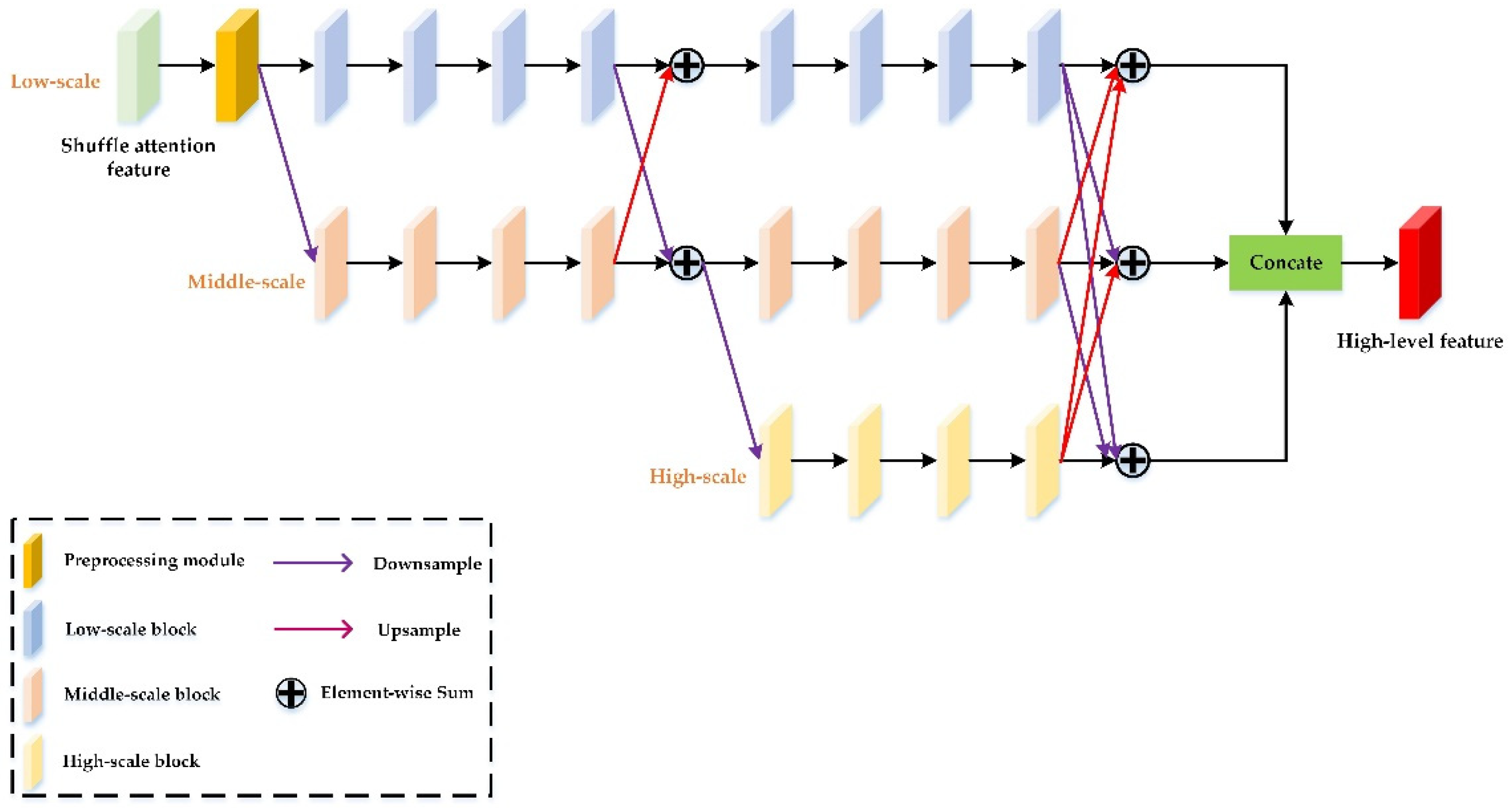
As the number of convolutional layers increases, different convolutional layers can capture features from fine to coarse. However, traditional CNNs simply pass the feature maps from one convolutional layer to the next convolutional layer, resulting in CNNs not making full use of the multiscale information to train networks. Therefore, we construct a context-aware spectral-spatial feature extraction module to achieve the utmost multiscale spectral-spatial features of scale invariance. The network structure of CHSFEM is displayed in Figure 3.

Here, the CHSFEM employs a “Horizontal-Vertical” sampling structure, which can capture the uniform scale spectral-spatial features from shallow to deep, as well as repeatedly fuse low, middle, and high three-scale features from different scale subnets to obtain multi-scale features. The CHSEFM realizes multiscale spectral-spatial feature of scale invariance in two dimensions. In the horizontal direction, the CHSFEM obtains the expressive depth spectral-spatial features at the same scale with dense connections. The dense connections can reuse spectral-spatial features, effectively increase the information flow, and lessen the negative effects of overfitting. In the vertical direction, we use downsampling and upsampling operations to generate low, middle, and high three-scale spectral-spatial feature maps, which can make the feature maps change between detailed and abstract. In addition, to ensure the integrity of spectral-spatial features, we design a communication mechanism between fine and coarse features, which complements the different information corresponding to low-scale, middle-scale, and high-scale parts. The CHSFEM is introduced in detail as follows.

First, we adopt a pre-processing module consisting of several bottleneck blocks to reduce training parameters and be conducive to extract more representative spectral-spatial features. Second, we start from a low-scale subnetwork as the first stage and gradually connect low-to-middle-to-high subnetworks in parallel one by one, forming new stages. Each subnetwork implements feature extraction in two dimensions. In the horizontal direction, the spectral-spatial features are captured by repeated $3\times 3$ convolution with dense connections at the same scale. The horizontal connections can reserve high-resolution HSI information and acquire scale invariant features. In the vertical direction, we employ downsampling and upsampling operations to generate different scale features. Then, multiscale spectral-spatial features at diverse levels are fused using elementwise summation to ensure that each network can tautologically obtain the information from other parallel networks. The vertical connects facilitate the HSI classification by producing more abstract features. Subsequently, we obtain three different scale features with context-aware information, and two of the smaller features are upsampled to the largest feature. Finally, we combine them by a concatenate operation to obtain the output of the CHSFEM.

2.4. Spectral-Spatial Frequency Attention Module

High-level spectral-spatial features usually contain more abundant and more abstract information, which is helpful for HSI classification. To compress the spectral channels and further achieve more discriminant and more plentiful features, we present the spectral-spatial frequency attention module, which can commendably complement the spectral-spatial features obtained from CHSFEM by introducing multiple frequency components. The network structure of SFAM is shown in Figure 4. The SFAM is described in detail in later sections.

2.4.1. Discrete Cosine Transform (DCT)

Specifically, the equation of two-dimensional (2D) DCT is indicated as follows:

$$B_{h,w}^{i,j}=\cos (\frac{\pi h}{H}(i+\frac{1}{2}))\cos (\frac{\pi w}{W}(j+\frac{1}{2}))$$

(9)

Next, the 2D DCT can be written as follows:

$$f_{h,w}^{2d}={\displaystyle \sum _{i=0}^{H-1}{\displaystyle \sum _{j=0}^{W-1}{x}_{i,j}^{2d}}}{B}_{h,w}^{i,j}$$

(10)

where $h\in \{0,1,2,\dots ,H-1\}$ and $w\in \{0,1,2,\dots ,W-1\}$. The 2D DCT frequency spectrum is represented by $f\in R^{H\times W}$. $x^{2d}\in R^{H\times W}$ is the input, $H$ refers to the height of the input, and $W$ denotes the width of the input. Then, the inverse 2D DCT can be expressed as follows:

$$x_{i,j}^{2d}={\displaystyle \sum _{h=0}^{H-1}{\displaystyle \sum _{w=0}^{W-1}{f}_{h,w}^{2d}}}{B}_{h,w}^{i,j}$$

(11)

where $i\in \{0,1,2,\dots ,H-1\}$ and $j\in \{0,1,2,\dots ,W-1\}$.

2.4.2. Multispectral Frequency Attention

First, we divide the input $X$ into many parts along the spectral dimension and use $[X^0,X^1,\dots ,X^{n-1}]$ to represent them, where $X\in R^{H\times W\times C^{\prime }},i\in \{0,1,2,\dots ,n-1\}$, $C^{\prime }=\frac{C}{n}$ and $C$ should be divisible by $n$. Second, each part is assigned a corresponding 2D DCT frequency component, and the output of 2D DCT can be used as the compressed results of SFAM as follows:

$$\begin{array}{cc}\hfill Fre{q}^i& =2DDC{T}^{u_i,v_i}(X^i)\hfill \\ & ={\displaystyle \sum _{h-0}^{H-1}{\displaystyle \sum _{w=0}^{W-1}{X}_{h_i,w_i}^i}}{B}_{h,w}^{u_i,v_i}\hfill \end{array}$$

(12)

where $[u_i,v_i]$ are the 2D DCT frequency component indices corresponding to $X^i$. The compressed vector is denoted by $Freq\in R^{C^{\prime }}$. Then, we use the concatenate operation to obtain the whole compressed vector as follows:

$$\begin{array}{cc}\hfill Freq& =compress(X)\hfill \\ & =([Fre{q}^0,Fre{q}^1,\dots ,Fre{q}^{n-1}])\hfill \end{array}$$

(13)

where $Freq\in R^C$ is the obtained multispectral vector. Additionally, the output of SFAM can be defined as follows:

$$output=sigmoid(FC(Freq))$$

(14)

2.4.3. Criteria for Choosing Frequency Components

It is vital to choose suitable frequency component indices $[u_i,v_i]$ for each $X^i$. To fulfil the SFAM, we adopt a two-step selection scheme to select frequency components. First, the importance of each frequency component is determined, and then we capture the effects of employing diverse numbers of frequency components. Sequentially, the results of each frequency component are evaluated. Finally, we choose the Top-k highest performance frequency components based on the evaluation results [52].

2.5. Cross-Connected Semantic Feature Extraction Module

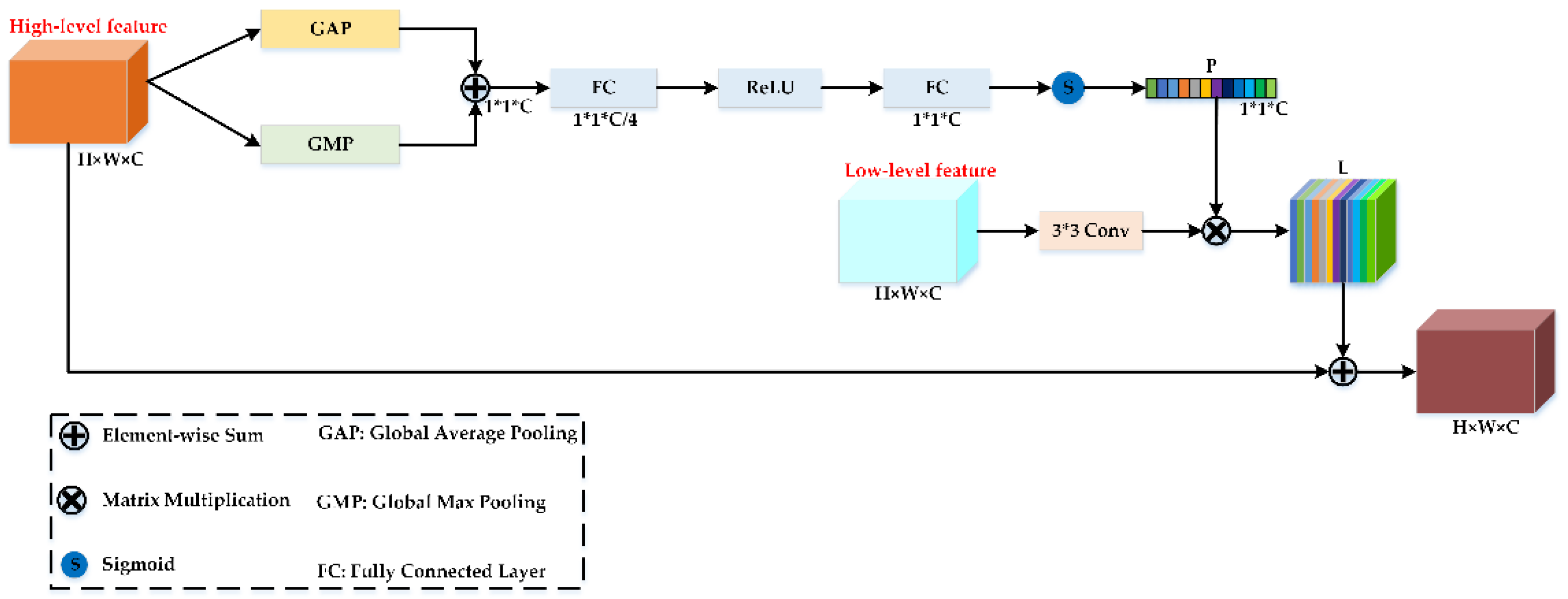
During the process of HSI classification, if the boundary of each category is not clearly defined, it may damage the classification accuracy. In addition, category information of HSI has a texture similar to that of its surrounding adjacent regions, which may aggravate the difficulty of HSI classification. To solve the above issues, we build the cross-connected semantic feature extraction module. The CSFEM can obtain high-level context cross-connected semantic features and fully exploit spectral-spatial shuffle attention features from the encoder phase to better guide more the diversified spectral-spatial frequency attention features, suppress noisy boundaries and restore category boundaries, while further strengthening the classification performance. Figure 5 exhibits the schematic diagram of the CSFEM.

First, we employ global average pooling and global max pooling to generate two different spectral-spatial descriptors, which are denoted by $F_{gap}$ and $F_{gmp}$. Second, two descriptors are aggregated using elementwise summation, which can learn the global context features and help to obtain more refined features. The gating module composed of two fully connected layers (FCs) and one ReLU activation function is adopted to reduce the complexity of the proposed DSFNet and aid generalization. After the sigmoid operation, we obtain the global context attention features $p\in R^{1\times 1\times C}$. The equation of $C$ can be provided as follows:

$$p=\sigma (W_1(\delta (W_0(F_{gap}+F_{gmp}))))$$

(15)

where $W_0\in R^{1\times 1\times (C/4)}$ and $W_1\in R^{1\times 1\times C}$ represent convolutional kernels of FCs. $\sigma$ refers to the sigmoid function. $\delta$ denotes the ReLU activation function. Subsequently, $3\times 3$ convolution is performed on the low-level feature to obtain $T\in R^{H\times W\times C}$. Next, matrix multiplication is performed between $P$ and $T$ to acquire $L\in R^{H\times W\times C}$. Finally, an elementwise summation is used between the high-level feature and $L$ to achieve the final output.

3. Experiments and Results

To qualitatively and quantitatively analyze the classification performance of the proposed method, we compare it with some state-of-the-art HSI classification methods on four public HSI datasets. We discuss several main factors influencing the classification performance of the proposed method, e.g., the number of training samples and the spatial size of input cube. In addition, to verify the effectiveness of the proposed method framework, we perform three ablation experiments on the four HSI datasets.

3.1. Experimental Datasets Description

To demonstrate the superiority of the proposed DSFNet, four benchmark datasets are used for the experiments.

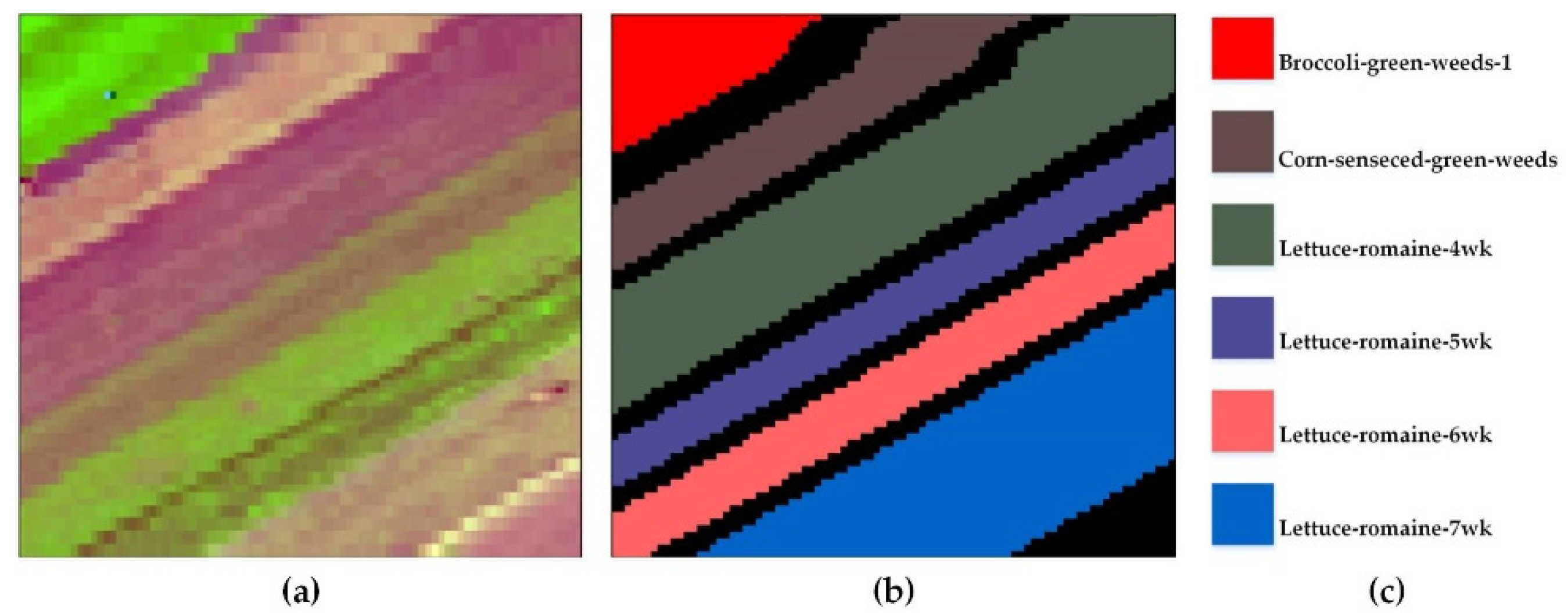
The Salinas-A Scene (SAC) dataset [53] is a small subscene of Salinas scene, gathered by an airborne visible infrared imaging spectrometer (AVIRIS) sensor over the Salinas Valley of California. It consists of 6 ground-truth categories and a spatial resolution of 3.7 m per pixel. The original SAC dataset is $83\times 86\times 224$, and its wavelength ranges from 0.4 to 2.5 µm. Since 20 bands with high moisture absorption are removed, the remaining 204 spectral bands can be used for HSI experiments.

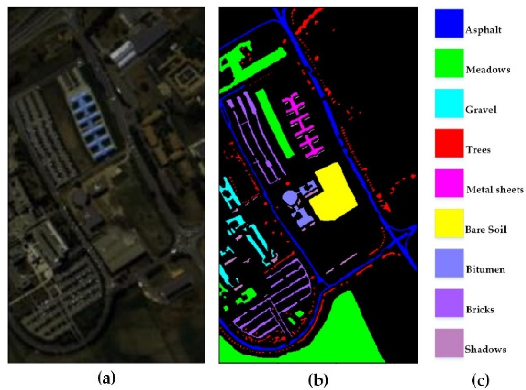
The University of Pavia (UP) [10] is acquired by a reflective optics system imaging spectrometer (ROSIS-03) sensor over the campus of the University of Pavia, Italy. It is composed of 9 ground-truth categories and a spatial resolution of 1.3 m per pixel. The original UP dataset is $610\times 340\times 105$, and its wavelength ranges from 0.43 to 0.86 µm. Due to the existence of a high amount of noise, the corrected UP dataset includes 103 bands.

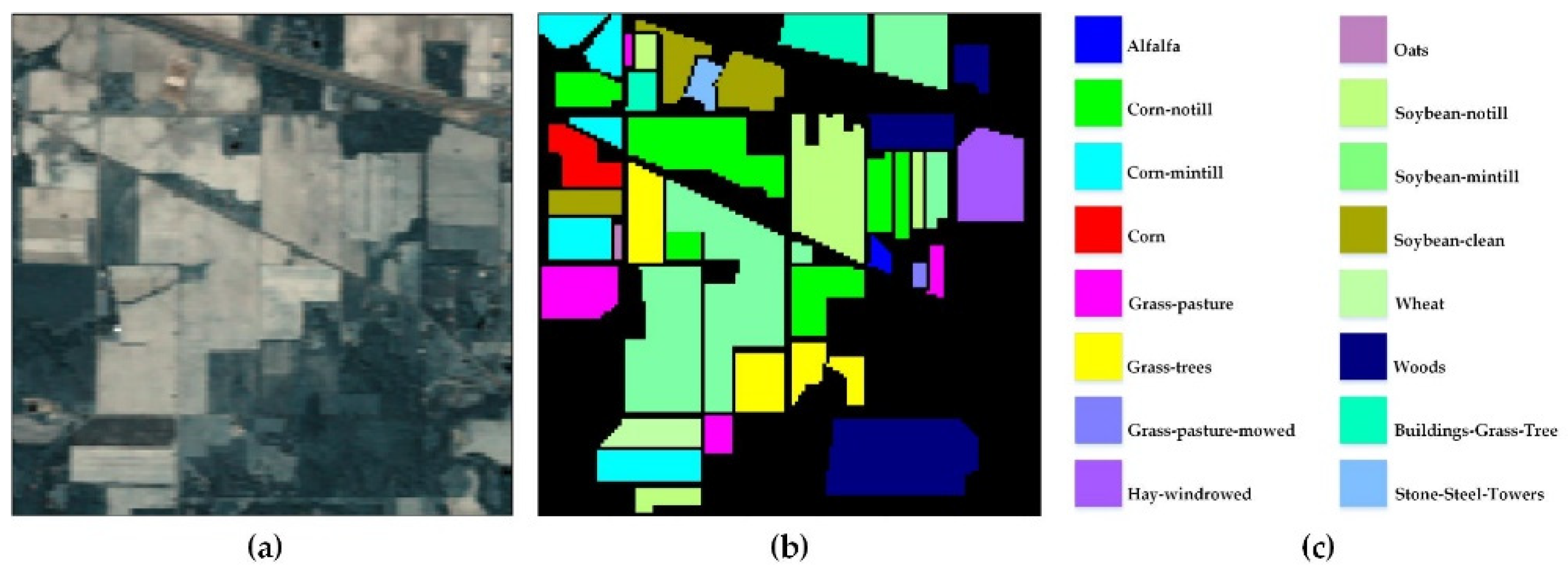
The India Pines (IP) dataset [10] is acquired by an airborne visible infrared imaging spectrometer (AVIRIS) sensor over the India Pine Forest pilot area of north-western Indiana. It consists of 16 ground-truth categories and a spatial resolution of 20 m per pixel. The original IP dataset is $145\times 145\times 224$, and its wavelength ranges from 0.2 to 2.4 µm. Because some spectral bands cannot be reflected by water, the corrected IP dataset includes 200 bands.

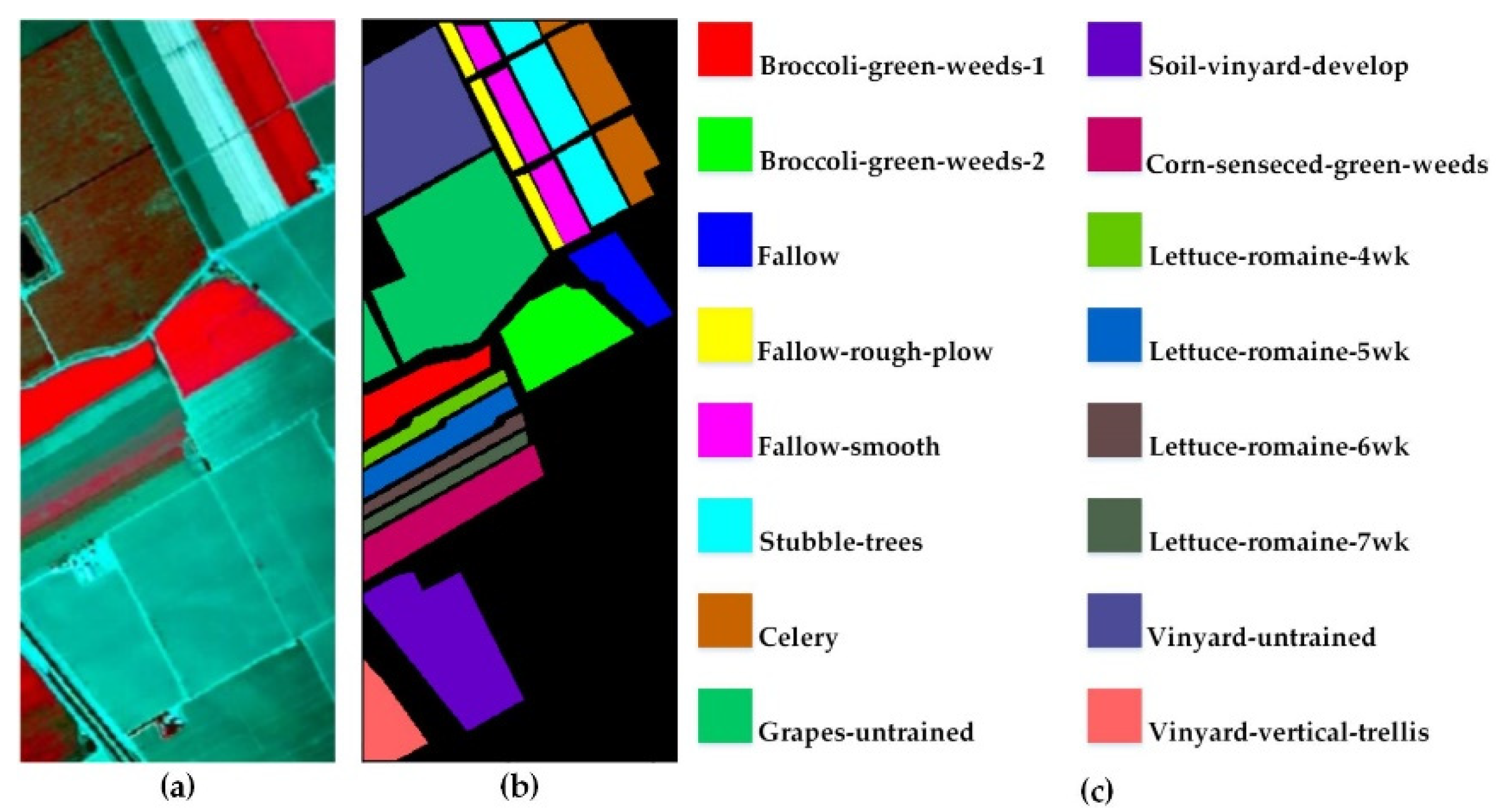
The Salinas (SA) dataset [54] is acquired by AVIRIS sensor over the Salinas Valley of California. It has 16 ground-truth categories and a spatial resolution of 3.7 m per pixel. The original SA dataset is $512\times 217\times 224$, and its wavelength ranges from 0.4 to 2.5 µm. After removing some spectral bands cannot be reflected by water, the corrected SA dataset includes 204 bands.

Table 1. Land cover class information for the SAC dataset.

No.	Class	Train	Test
1	Broccoli-green-weeds-1	40	351
2	Corn-senseced-green-weeds	135	1208
3	Lettuce-romaine-4wk	62	554
4	Lettuce-romaine-5wk	153	1372
5	Lettuce-romaine-6wk	68	606
6	Lettuce-romaine-7wk	80	719
Total		538	4810

,

Table 2. Land cover class information for the UP dataset.

No.	Class	Train	Test
1	Asphalt	664	5967
2	Meadows	1865	16,784
3	Gravel	210	1889
4	Trees	307	2757
5	Metal sheets	135	1210
6	Bare Soil	503	4526
7	Bitumen	133	1197
8	Bricks	369	3313
9	Shadows	95	852
Total		4281	38,495

,

Table 3. Land cover class information for the IP dataset.

No.	Class	Train	Test
1	Alfalfa	10	36
2	Corn-notill	286	1142
3	Corn-mintill	166	664
4	Corn	48	189
5	Grass-pasture	97	386
6	Grass-trees	146	584
7	Grass-pasture-mowed	6	22
8	Hay-windrowed	96	382
9	Oats	4	16
10	Soybean-notill	195	777
11	Soybean-mintill	491	1964
12	Soybean-clean	119	474
13	Wheat	41	164
14	Woods	253	1012
15	Buildings-Grass-Tree	78	308
16	Stone-Steel-Towers	19	74
Total		2055	8194

and

Table 4. Land cover class information for the SA dataset.

No.	Class	Train	Test
1	Broccoli-green-weeds-1	201	2825
2	Broccoli-green-weeds-2	373	3353
3	Fallow	198	1178
4	Fallow-rough-plow	140	154
5	Fallow-smooth	268	2410
6	Stubble-trees	396	3563
7	Celery	358	3221
8	Grapes-untrained	1128	10,143
9	Soil-vinyard-develop	621	5582
10	Corn-senseced-green-weeds	328	2950
11	Lettuce-romaine-4wk	107	961
12	Lettuce-romaine-5wk	193	1734
13	Lettuce-romaine-6wk	92	824
14	Lettuce-romaine-7wk	107	963
15	Vinyard-untrained	727	6541
16	Vinyard-vertical-trellis	181	1626
Total		5418	48,711

show the total number of samples of each category for each HSI dataset, and Figure 6, Figure 7, Figure 8 and Figure 9 list false-color images and ground-truths of the four datasets.

3.2. Experimental Evaluation Indications

We employ the OA, AA and Kappa coefficient as the evaluation indexes to evaluate the classification performance of the proposed DSFNet.

The confusion matrix (CM) can reflect the classification results, which is the basis for people to understand other classification evaluation indexes of HSI. Assuming that there are $n$ kinds of ground objects, and the equation of the CM with the size of $n\times n$ is as follows:

$$C=\left[\begin{array}{llll}{c}_{11}& c_{12}& \dots & c_{1n}\\ c_{21}& c_{22}& \dots & c_{21}\\ \dots & \dots & \dots & \dots \\ c_{n1}& c_{n2}& \dots & c_{nn}\end{array}\right]$$

(16)

where element $c_{ij}$ represents that the number of samples in category $i$ has been classified as class $j$. ${\displaystyle \sum _i^n{c}_{ij}}$ and ${\displaystyle \sum _j^n{c}_{ij}}$ denote the number of samples in category $i$ and the number of samples in category $j$ respectively.

The overall accuracy (OA) is the proportion of correctly classified samples in the total samples. The OA is defined as follows:

$$OA=\frac{{\displaystyle \sum _{i=1}^n{c}_{ii}}}{{\displaystyle \sum _{j=1}^n{\displaystyle \sum _{i=1}^n{c}_{ij}}}}$$

(17)

The average accuracy (AA) represents the ratio between the total sample numbers of each category and the correctly classified sample numbers. The AA is defined as follows:

$$AA=\frac{1}{n}\times {\displaystyle \sum _{i=1}^n\frac{c_{ii}}{c_{ij}}}$$

(18)

The Kappa coefficient measures the consistency between the ground-truth and the classification results. The Kappa is defined as follows:

$$Kappa=\frac{N{\displaystyle \sum _{i=1}^n{c}_{ii}}-{\displaystyle \sum _{i=1}^n({\displaystyle \sum _{j=1}^n{c}_{ij}\times {\displaystyle \sum _{i=1}^n{c}_{ij}}})}}{N^2-{\displaystyle \sum _{i=1}^n({\displaystyle \sum _{j=1}^n{c}_{ij}\times {\displaystyle \sum _{i=1}^n{c}_{ij}}})}}$$

(19)

3.3. Experimental Settings

For the IP dataset, we randomly choose 20% of the samples as the training set, and the remaining 80% of the samples are utilized as the test set. For other three experimental datasets, we randomly choose 10% of the samples as the training set, and the remaining 90% of the samples are utilized as the test set. Due to the sample numbers in the different datasets are diverse, different batch sizes are set for the four datasets. The batch sizes of the SAC dataset, the UP dataset, the IP dataset, and the SA dataset are 16, 64, 16, and 128, respectively. In addition, the training epochs of the SAC dataset, the UP dataset, the IP dataset, and the SA dataset are 100, 25, 200, and 50, respectively. Adopting Adam as the optimizer to make the model converge rapidly, the learning rates of the SAC dataset, the UP dataset, the IP dataset, and the SA dataset are 0.0005, 0.0005, 0.0001, and 0.0005, respectively.

The hardware environment of the experiments is a server with an NVIDIA GeForce RTX 2060 SUPER GPU and Intel i-7 9700F CPU. In addition, the software platform is based on TensorFlow 2.3.0, Keras 2.4.3, CUDA 10.1 and Python 3.6.

3.4. Framework Parameter Settings

In the proposed DSFNet, five vital parameters affect the performance of HSI classification, i.e., the number of training samples, the spatial size of image cube, the number of principal components, the number of groups for SSAM, and the number of frequency components for SFAM. In this part, we discuss the influences of these five parameters on HSI classification when setting different values.

3.4.1. Sensitivity to the Number of Training Samples

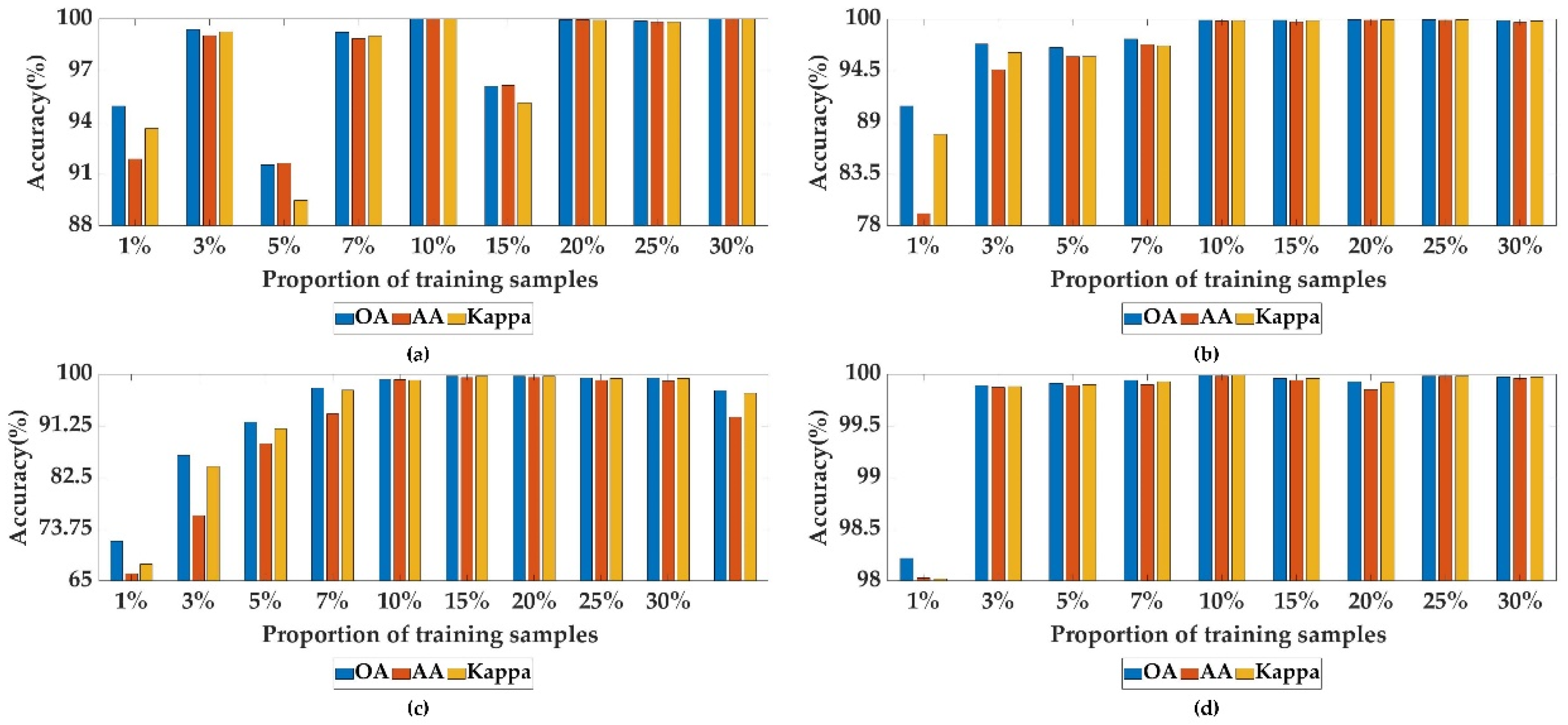
To explore the sensitivity of the proposed DSFNet to different numbers of training samples, we randomly select 1%, 3%, 5%, 7%, 10%, 15%, 20%, 25% and 30% of the samples as the training set, and the corresponding remaining samples as the test set. Figure 10 shows the corresponding classification results of diverse training sample numbers on the SAC, UP, IP and SA datasets. In general, as the proportion of training samples increases, the OA, AA and Kappa of the DSFNet also gradually increase on the four datasets. Specifically, for SAC, UP and IP datasets, when the proportion of training samples is 1%, 3%, 5% or 7%, for SA dataset, when the proportion of training samples is 1%, we can clearly see that the classification performance is not good, because random selection of samples results in some sample categories not being selected. When the proportion of training samples is 10%, 15% or 20%, the OA, AA and Kappa of the DSFNet on the four datasets are almost all more than 96%. When the proportion of training samples is 25% or 30%, the OA, AA and Kappa of the DSFNet on the four datasets are all over 99%. Because the SAC and IP datasets have relatively few labeled samples, the proportion of training samples greatly influences the classification performance of the two datasets. In contrast, the UP and SA datasets have a mass of labeled samples, which can obtain fine classification performance for small labeled samples. Therefore, to obtain the unexceptionable classification results of the DSFNet, we randomly choose 20% of the samples as the training set, and the remaining 80% of the samples as the test set for the IP dataset. For the other three experimental datasets, we randomly choose 10% of the samples as the training set, and the remaining 90% of the samples are utilized as the test set.

3.4.2. Sensitivity to the Spatial Size of Input Cube

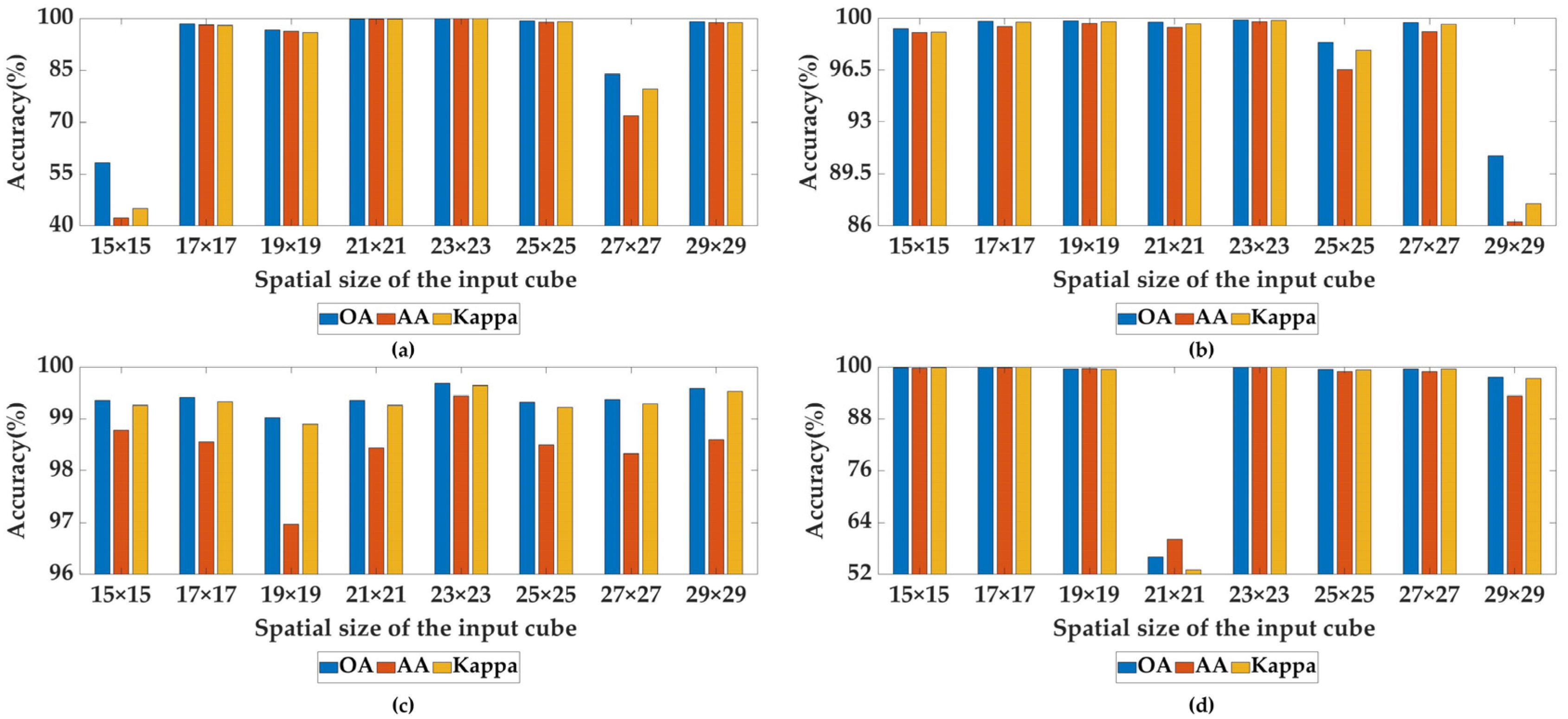
The classification performance of the proposed DSFNet is sensitive to the spatial size of image cube. Although the larger spatial size of input cube contains richer contextual information, the information proportion of the center pixel among pixels in the input cube is lower. The smaller spatial size of input cube can reduce computational complexity and include less noise, but an inadequate receptive field leads to the loss of information and damage to the classification ability. Therefore, we utilize eight different spatial sizes of image cube to find the optimal cube, which are set $15\times 15$, $17\times 17$, $19\times 19$, $21\times 21$, $23\times 23$ $25\times 25$, $27\times 27$ and $29\times 29$. Figure 11 shows the influences of diverse patch spatial sizes on the four HSI datasets. We can clearly see that when the spatial size of image cube is $23\times 23$, the evaluation indexes reach the optimal values on the IP and UP datasets. Therefore, the spatial size of $23\times 23$ is regarded as the most suitable spatial size of the DSFNet’s input cube for the IP and UP datasets. When the spatial size of image cube is $21\times 21$ or $23\times 23$, the SAC dataset achieves much better classification performance. Because the OA, AA and Kappa of latter all reach to 100%, which are superior to the former, hence the spatial size of $23\times 23$ is decided as the most suitable spatial size of the DSFNet’s input cube for the SAC dataset. For the SA dataset, when the spatial size of image cube is $21\times 21$, we can find that compared with other conditions, the evaluation indexes of OA, AA and Kappa of our proposed DSFNet are very low. The situation may be the spatial size of $21\times 21$ contains too much background information and less contextual information. As shown in Figure 11d, it is evident that when the spatial size of input cube is $23\times 23$, the OA, AA and Kappa of the DSFNet are superior to the others, which are all over 99.98%, we choose the spatial size of $23\times 23$ as the most suitable spatial size of the DSFNet’s input cube on the SA dataset.

3.4.3. Sensitivity to the Number of Principal Components

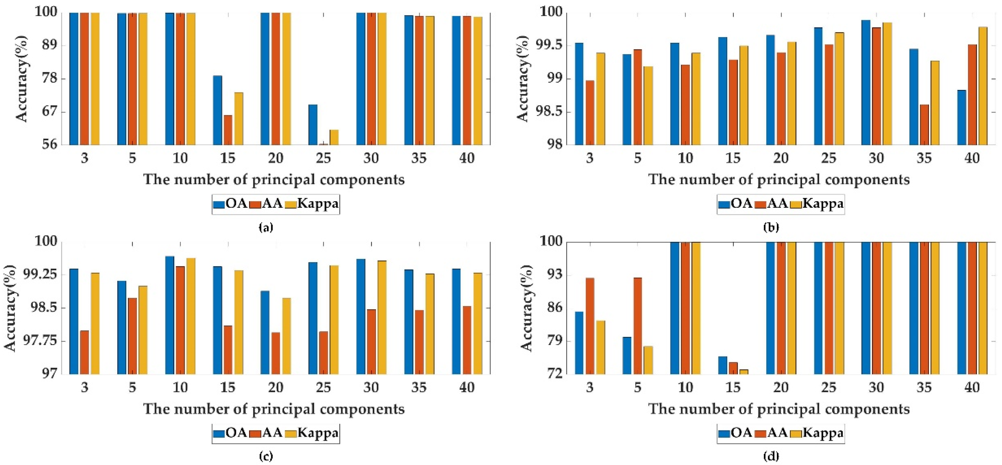
We set the different numbers of principal components to analyze its effect on the three HSI datasets, i.e., {3, 5, 10, 15, 20, 25, 30, 35, 40}. From Figure 12b,c, we can clearly see that, when the number of principal components is 30, the UP dataset possesses the best evaluation indexes, when the number of principal components is 10, the IP dataset obtain the optimal classification performance. Therefore, we set the number of principal components to 30 for the UP dataset and 10 for the IP dataset. As shown in Figure 12a, it is obvious that 20 or 30 principal components show the best classification performance, of which all the evaluation indications reach 100%. Considering the training time and parameters, the number of principal components set to 20 is utilized for the SAC dataset. As shown in Figure 12d, when the number of principal components is 15, we can find that compared with other conditions, the evaluation indexes of OA, AA and Kappa on SA dataset are very low. This may be because although the 15 bands retained by PCA contain a large amount of important information of HSI, there is a strong correlation between these bands, so there is redundancy among them, which reduces the classification performance of our proposed method. From Figure 12d, it is obvious that the SA dataset achieves good evaluation indications in many cases. when the number of principal components is 30, the OA, AA and Kappa of the DSFNet are superior to the others, which are all over 99.98%, the number of principal components to 30 is chosen for the SA dataset.

3.4.4. Sensitivity to the Number of Groups for SSAM

The SSAM can not only extract local and global spectral and spatial features separately but can aggregate the large short-range correlation between spectral and spatial information, as well as further modeling the large long-range interdependency of spectral and spatial data. The number of groups for SSAM has a large impact on the classification accuracy of the three HSI datasets. If the number of groups is too small, the spectral-spatial extraction is not sufficient and results in the loss of important information. If the number of groups is too large, the model needs more training parameters and longer training time, resulting in the aggravated computational burden and the degradation of the model. Therefore, the classification performance is analyzed to find the optimal number of groups for SSAM. 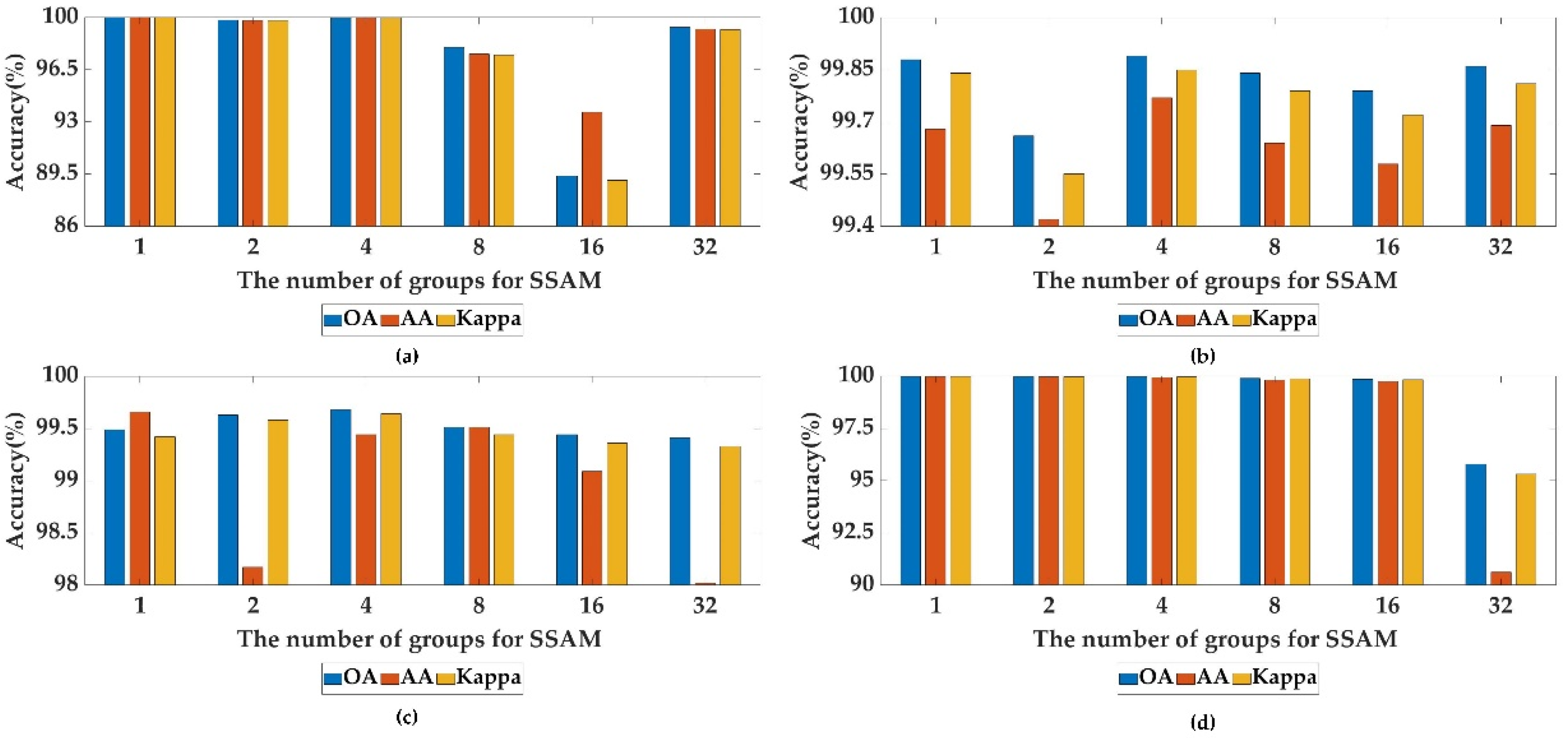Figure 13 shows the results when the number of groups is 1, 2, 4, 8, 16 and 32 on the four HSI datasets. As shown in Figure 13b,c, we can clearly see that when the number of groups is 4, the UP and IP datasets achieve much better classification accuracy. As shown in Figure 13a, it is evident that when the number of groups is 1, the OA, AA and kappa all reach 100. Therefore, the most appropriate number of groups is 1, 4 and 4 for the SAC, UP and IP datasets, respectively. As shown in Figure 13d, we can obviously find that all evaluation indexes of other conditions exceed 99.5%, except for the case where the number of groups is 32. Considering the cost and training time, we set the number of groups to 1 for the SA dataset.

3.4.5. Sensitivity to the Number of Frequency Components for SFAM

To investigate the effects of different numbers of frequency components for SFAM, eight various numbers of frequency components are adopted to find the optimal one, i.e., {1, 2, 4, 8, 16, 32, 64, 128}. Figure 14 shows the influences of different frequency components on the four HSI datasets. From Figure 14b,c, it is obvious that when the number of frequency components is 16, the UP dataset and IP dataset have a notable classification performance gain compared with the others. As shown in Figure 14a, when the number of frequency components is 16, the OA, AA and Kappa are the beat, all attaining 100%. From Figure 14d, it is obviously seen that all evaluation indexes of other conditions exceed 99%, except for the case where the number of frequency components is 64. In terms of the training time and computational expense, the frequency components of 2 is more proper choice for SA dataset. The experimental results demonstrate that it is necessary to adopt the appropriate number of frequency components to refine the captured high-level spectral-spatial features. Therefore, we set the number of frequency components to 16, 16, 16, and 2 for the SAC dataset, UP dataset, IP dataset, and SA dataset, respectively.

3.5. Comparisons with the State-of-the-Art Method

To evaluate the effectiveness of the proposed DSFNet, several classical and advanced classification methods are selected, including: support vector machine (SVM), random forest (RF), multinomial logistic regression (MLR), deep convolutional neural networks (1DCNN) [34], semi-supervised convolutional neural network (2DCNN) [55], image classification and band selection (3DCNN) [56], context deep CNN (2D_3D_CNN) [57], residual spectral-spatial attention network (RSSAN) [48], spectral-spatial attention network (SSAN) [58], multiattention fusion network (MAFN) [59], dual-channel residual network (DCRN) [60], dimension reduction on hybrid CNN (DRCNN) [61], 3-D–2-D CNN feature hierarchy (HybridSN) [62], and two-stream convolutional neural network (TSCNN) [63]. To achieve fair comparison results, our proposed DSFNet and compared methods adopt the same number of training samples: 10%, 10%, 20%, and 10% for the SAC dataset, the UP dataset, the IP dataset, and the SA dataset. The classification results of the DSFNet and the compared methods on the four experimental datasets are shown in

Table 5. Classification results on the SAC dataset.

No.	SVM	RF	MLR	1D_CNN	2D_CNN	3D_CNN	2D_3D_CNN	RSSAN	SSAN	MAFN	DCRN	DRCNN	HybridSN	TSCNN	DSFNet
1	100.00	100.00	100.00	61.78	23.60	99.15	100.00	100.00	96.16	100.00	100.00	100.00	100.00	100.00	100.00
2	69.02	73.75	99.75	84.52	100.00	97.66	98.45	97.26	100.00	100.00	99.65	99.18	100.00	99.83	100.00
3	100.00	0.00	99.80	97.52	95.92	100.00	99.82	100.00	100.00	99.45	91.18	100.00	100.00	100.00	100.00
4	99.62	92.44	69.51	97.93	100.00	99.93	99.56	98.99	99.27	99.02	79.95	96.67	96.42	95.21	100.00
5	100.00	96.18	100.00	99.37	100.00	97.85	100.00	100.00	99.33	61.66	76.88	100.00	100.00	100.00	100.00
6	100.00	98.74	99.72	100.00	99.86	100.00	100.00	96.51	97.82	89.99	100.00	100.00	100.00	100.00	100.00
OA (%)	88.70	87.95	87.45	90.19	75.90	99.04	99.46	98.46	99.09	90.96	88.52	98.84	98.94	98.52	100.00
AA (%)	82.63	82.39	83.29	90.40	77.14	98.99	99.38	96.50	99.03	93.67	82.55	97.82	98.60	98.05	100.00
Kappa (%)	85.61	84.56	83.89	87.76	70.99	98.80	99.32	98.09	98.86	88.84	85.43	98.54	99.67	98.15	100.00

The red font highlights which mechanic works best. The blue font does contrast test, our proposed method achieves the highest classification accuracy.

,

Table 6. Classification results on the UP dataset.

No.	SVM	RF	MLR	1D_CNN	2D_CNN	3D_CNN	2D_3D_CNN	RSSAN	SSAN	MAFN	DCRN	DRCNN	HybridSN	TSCNN	DSFNet
1	82.51	61.02	51.83	91.15	99.92	94.53	98.55	95.36	99.00	99.98	98.46	99.24	98.54	99.67	99.75
2	6.09	70.21	69.97	97.54	99.80	99.57	98.20	97.17	99.58	97.95	99.15	100.00	99.99	98.23	99.96
3	53.39	0.00	0.00	93.11	99.39	96.39	94.10	90.81	98.22	72.75	99.14	98.43	94.26	99.95	99.95
4	84.41	95.21	98.59	95.29	99.23	98.69	98.20	95.87	99.12	100.00	89.04	98.70	99.32	99.81	99.96
5	100.00	0.00	100.00	98.85	100.00	99.51	99.82	97.82	100.00	70.64	85.88	98.37	96.26	99.90	99.92
6	46.01	67.55	68.8	97.21	100.00	99.58	100.00	98.82	99.93	96.09	100.00	99.96	99.56	99.93	99.96
7	59.87	0.00	0.00	99.24	99.83	97.95	90.82	85.20	94.55	99.45	96.30	98.68	99.44	99.67	99.42
8	65.22	55.57	45.55	88.64	86.50	95.69	97.01	88.16	97.98	77.47	98.85	94.30	88.25	97.93	99.73
9	100.00	0.00	0.00	91.43	97.60	99.33	96.70	96.02	99.61	99.40	93.09	99.75	98.08	100.00	100.00
OA (%)	62.96	67.50	66.41	95.36	98.42	98.16	97.92	95.67	99.14	93.63	98.46	99.10	98.09	98.94	99.89
AA (%)	41.33	34.26	39.88	91.64	96.46	96.28	97.19	94.03	98.25	92.43	94.30	97.97	95.10	96.84	99.77
Kappa (%)	45.12	52.43	50.45	93.81	97.91	97.55	97.23	96.78	98.63	91.58	96.94	98.81	97.47	98.59	99.85

The red font highlights which mechanic works best. The blue font does contrast test, our proposed method achieves the highest classification accuracy.

,

Table 7. Classification results on the IP dataset.

No.	SVM	RF	MLR	1D_CNN	2D_CNN	3D_CNN	2D_3D_CNN	RSSAN	SSAN	MAFN	DCRN	DRCNN	HybridSN	TSCNN	DSFNet
1	92.31	100.00	57.14	92.86	100.00	97.06	90.00	89.74	87.80	100.00	100.00	97.22	100.00	100.00	100.00
2	64.25	63.13	61.06	73.51	72.96	93.36	95.95	97.94	98.33	81.75	86.99	98.59	98.69	95.72	99.48
3	67.11	68.09	65.84	95.19	100.00	97.63	95.94	97.92	99.53	87.14	58.16	98.04	99.85	98.66	99.25
4	52.50	55.00	45.70	98.94	100.00	91.46	90.72	99.47	100.00	88.24	97.06	95.29	99.47	97.47	98.95
5	84.63	86.67	67.27	93.70	98.42	97.70	98.71	99.48	99.47	98.21	89.57	96.98	98.46	93.67	98.72
6	90.58	89.44	87.30	97.93	99.62	99.14	97.82	97.64	99.83	98.63	95.69	99.13	100.00	98.48	100.00
7	85.71	90.00	89.47	100.00	100.00	100.00	100.00	100.00	100.00	100.00	0.00	100.00	100.00	0.00	100.00
8	95.14	88.22	91.39	100.00	100.00	99.74	98.71	100.00	100.00	91.83	100.00	100.00	98.71	100.00	100.00
9	28.57	0.00	0.00	100.00	100.00	100.00	100.00	100.00	77.78	0.00	0.00	100.00	100.00	0.00	100.00
10	71.99	71.21	65.93	96.11	100.00	98.57	99.46	99.87	99.87	95.19	68.45	98.44	99.74	100.00	100.00
11	69.86	72.01	63.44	95.39	94.18	97.50	99.37	98.57	98.00	89.22	93.56	98.93	99.04	99.90	99.85
12	67.05	54.93	47.94	92.96	97.50	98.29	94.51	93.71	98.30	88.32	77.42	96.13	97.23	92.40	98.96
13	90.45	91.41	92.86	100.00	100.00	100.00	100.00	100.00	95.91	96.47	65.60	99.39	100.00	100.00	100.00
14	86.16	84.26	86.82	99.00	100.00	99.50	98.81	99.90	100.00	94.49	97.56	99.12	99.80	99.90	100.00
15	71.36	66.53	68.80	87.18	100.00	98.98	91.59	89.02	98.40	94.97	89.23	99.34	99.68	100.00	100.00
16	100.00	100.00	95.53	95.52	93.42	92.21	91.36	95.65	86.50	93.42	0.00	97.33	91.30	100.00	100.00
OA (%)	74.67	73.92	70.04	91.92	93.10	97.46	97.45	98.05	98.69	92.87	84.28	98.51	99.13	98.28	99.68
AA (%)	69.18	61.06	62.13	82.84	87.24	93.24	95.57	98.11	97.77	77.65	63.34	97.58	98.12	84.09	99.44
Kappa (%)	70.86	70.16	65.41	90.75	92.09	97.10	97.10	97.78	98.51	91.83	82.10	98.30	99.01	98.04	99.64

The red font highlights which mechanic works best. The blue font does contrast test, our proposed method achieves the highest classification accuracy.

and

Table 8. Classification results on the SA dataset.

No.	SVM	RF	MLR	1D_CNN	2D_CNN	3D_CNN	2D_3D_CNN	RSSAN	SSAN	MAFN	DCRN	DRCNN	HybridSN	TSCNN	DSFNet
1	100.00	92.48	0.00	100.00	100.00	100.00	100.00	99.94	100.00	99.83	100.00	99.94	100.00	100.00	100.00
2	99.73	98.01	64.66	96.54	100.00	100.00	100.00	98.76	100.00	100.00	100.00	100.00	100.00	100.00	100.00
3	78.28	56.51	83.35	98.73	100.00	100.00	99.94	98.12	100.00	100.00	99.94	99.83	100.00	100.00	100.00
4	99.78	97.86	100.00	98.46	99.20	98.43	99.76	98.92	78.77	99.21	97.88	99.84	95.58	71.05	100.00
5	96.43	60.66	51.92	83.33	100.00	99.42	99.75	99.48	99.38	99.89	9946	99.71	100.00	100.00	100.00
6	100.00	100.00	99.97	99.72	99.92	100.00	99.55	99.64	100.00	86.44	99.89	100.00	99.89	100.00	100.00
7	100.00	99.65	64.53	100.00	100.00	100.00	100.00	99.05	100.00	99.75	100.00	100.00	100.00	100.00	100.00
8	30.39	41.40	59.21	88.71	78.81	86.03	100.00	99.99	99.99	99.22	100.00	99.96	99.97	99.15	99.99
9	99.40	90.16	54.31	100.00	100.00	99.96	100.00	99.66	99.96	100.00	100.00	98.95	100.00	90.18	100.00
10	92.85	0.00	54.87	99.97	100.00	96.75	99.86	99.53	100.00	100.00	99.93	99.86	97.97	100.00	99.97
11	99.25	0.00	0.00	100.00	100.00	99.90	100.00	99.90	100.00	99.79	100.00	98.26	100.00	100.0	100.00
12	98.82	0.00	0.00	92.70	99.88	100.00	100.00	98.34	100.00	100.00	98.30	100.00	66.74	100.00	100.00
13	100.00	0.00	0.00	96.68	100.00	98.68	100.00	98.05	99.76	94.50	98.68	99.40	0.00	100.00	99.52
14	100.00	0.00	0.00	81.53	100.00	100.00	100.00	99.90	99.07	100.00	100.00	98.06	88.60	94.46	100.00
15	50.72	0.00	0.01	90.95	99.61	100.00	91.89	81.15	99.35	100.00	90.50	99.94	99.47	99.68	100.00
16	100.00	0.00	0.00	100.00	100.00	99.88	99.63	99.08	100.00	96.67	100.00	100.00	100.00	100.00	100.00
OA (%)	58.64	64.34	61.20	94.29	94.34	96.32	98.74	96.38	99.18	98.43	98.41	99.74	97.64	97.37	99.99
AA (%)	4782	49.53	42.15	93.78	96.54	97.87	99.55	98.78	98.94	97.93	98.97	99.56	92.05	93.08	99.98
Kappa (%)	51.51	58.50	55.64	93.64	93.66	95.89	98.60	95.98	99.08	98.25	98.23	99.71	97.37	97.07	99.99

The red font highlights which mechanic works best. The blue font does contrast test, our proposed method achieves the highest classification accuracy.

, respectively. In addition, by comparing the proposed DSFNet with the diverse classification methods, we can obtain the following conclusions from four different perspectives.

(1)

SVM, RF and MLR are the traditional classification methods, whereas 1D_CNN, 2D_CNN, 3D_CNN, 2D_3D_CNN, RSSAN, SSAN, MAFN, DCRN, DRCNN, HybridSN, TSCNN and our proposed DSFNet are based on deep learning. From Table 5, Table 6, Table 7 and Table 8, we can find that compared with the traditional classification methods, the classification methods utilizing deep learning obtain better performances, except the classification results of the 2D_CNN on the SAC dataset. This is because traditional classification methods rely on manual feature extraction with limited represent ability. Nevertheless, deep learning methods can automatically capture high-level hierarchical spectral-spatial features from HSI. In addition, our proposed DSFNet achieves admirable classification accuracy compared with the traditional classification methods and the other deep learning classification methods. For instance, the proposed method obtains 100% OA, 100% AA, and 100% Kappa on the SAC dataset, which are 11.30%, 17.37% and 14.39% higher than SVM.

(2)

The TSCNN classification method incorporates the SE concept into the model to improve the spectral-spatial feature extraction ability by emphasizing automatically informative features and suppressing the less useful ones. However, the method only considers the mutual attention dependence between different channels and does not consider the spatial attention relation between any two pixels. The MAFN employs a spatial attention module and band attention module to reduce the influence of interfering pixels and redundant bands. The RSSAN designs a spectral attention module for spectral band selection and a spatial module to select spatial information. The SSAN builds a spectral–spatial attention network to obtain discriminative spectral and spectral information. Although the MAFN extracts multiattention spectral and spatial features, and the RSSAN achieve meaningful spectral-spatial information and the SSAN can suppress the effects of interfering pixels, the large long-term interdependence relationship between spatial and spectral features dose is not captured. Compared with the TSCNN, MAFN, RSSAN and SSAN, our proposed method extracts local and global spectral and spatial independent features, while also aggregating the large short-range interdependency of spectral and spatial features, further modelling the large long-range correlation between spectral and spatial data. For example, our proposed DSFNet achieves 99.99% OA, 99.98% AA, and 99.99% Kappa on the SA dataset, which are 2.62%, 6.90% and 2.92% higher than TSCNN, 4.56%, 2.05% and 1.74% higher than MAFN, 3.61%, 1.20% and 4.01% higher than RSSAN, 3.61%, 0.81% and 0.91% higher than SSAN. Compared with other deep learning classification methods without the attention module, our proposed method shows superiority for HSI classification. These results also demonstrate that our proposed spectral-spatial shuffle attention module and spectral-spatial frequency attention module are very helpful and extremely effective for HSI classification.

(3)

The TSCNN, MAFN and DCRN deep learning classification methods use a two-stream CNN architecture for HSI analysis, i.e., the spectral feature extraction stream and spatial feature extraction stream. The former captures spectral information, and the latter extracts spatial information. The final joint spectral-spatial features are obtained by a fusion scheme. Although these methods achieve good classification performance, they only employ simple concatenation operations or elementwise summation to fuse independent spectral and spatial features, neglecting the close correlations between spectral and spatial information. Our proposed method is highly competitive with the above methods, which utilizes two SSAMs, one CHSFEM, three SFAMs and four CSFEMs to directly capture high-level spectral-spatial-semantic joint features and model the large long-range interdependency of spectral and spatial joint information. In addition, the results show that our proposed method has better performance than deep learning methods using a simple fusion scheme because the DSFNet contains more expressive joint spectral-spatial features and further updates the interdependency of spectral and spatial data.

(4)

The DSFNet has a strong ability to execute HSI classification with limited labeled samples. As shown in Table 5, Table 6, Table 7 and Table 8, the OA, AA and Kappa of the proposed method exhibit much better classification accuracy compared with other classification methods. In addition, on the UP dataset IP dataset and SA dataset, the evaluation indexes exceed 99%; on the SAC dataset, the evaluation indexes reach 100%. With insufficient labeled samples, our proposed method can still fully extract the joint spectral-spatial features and improve the classification performance. 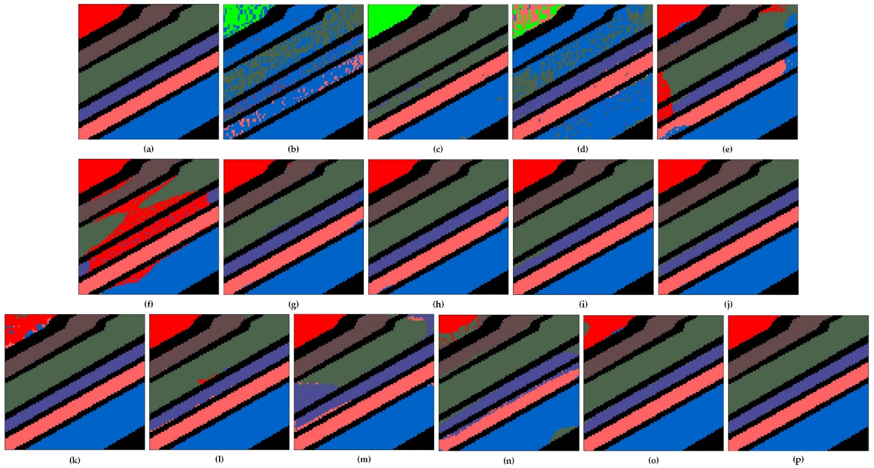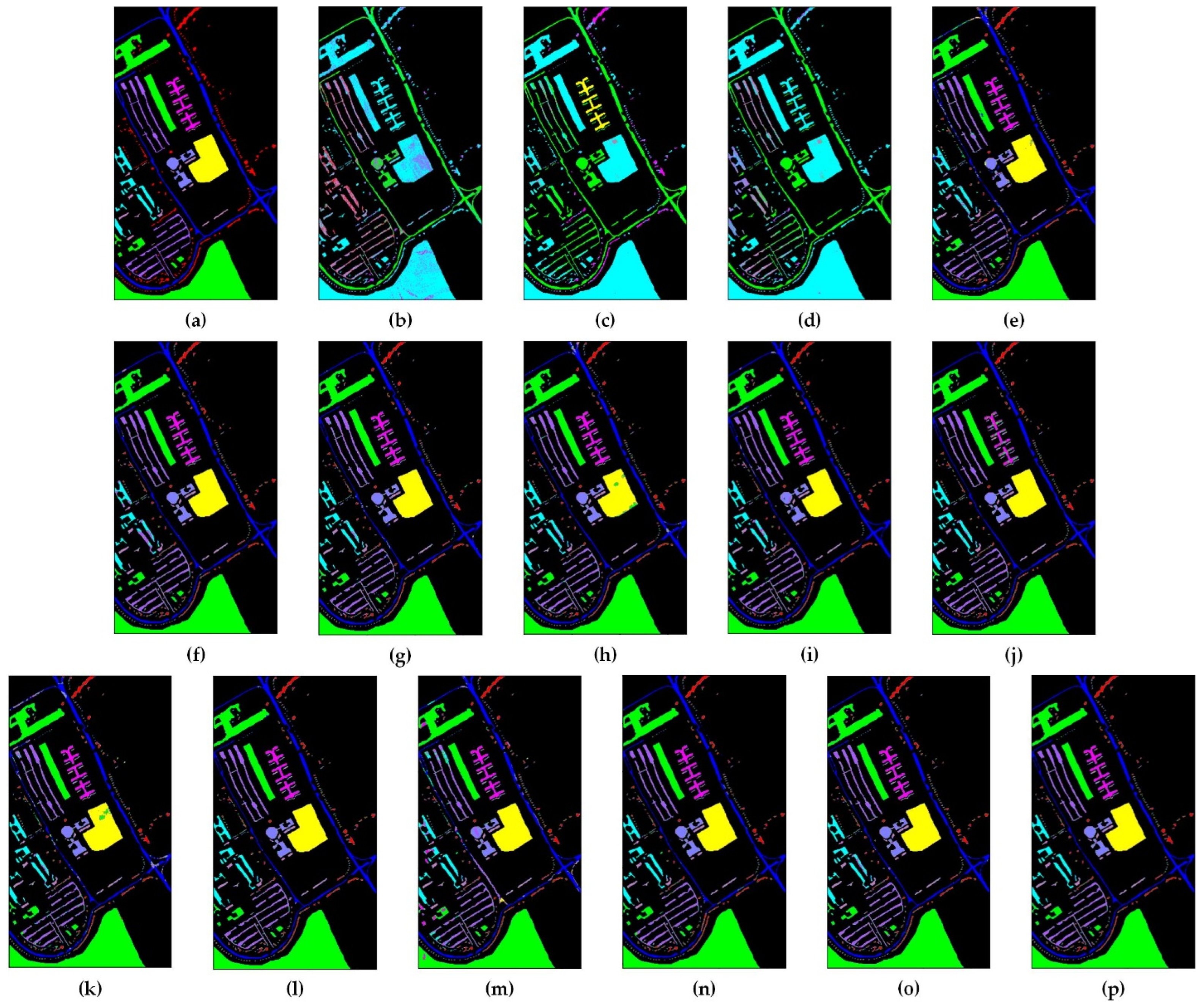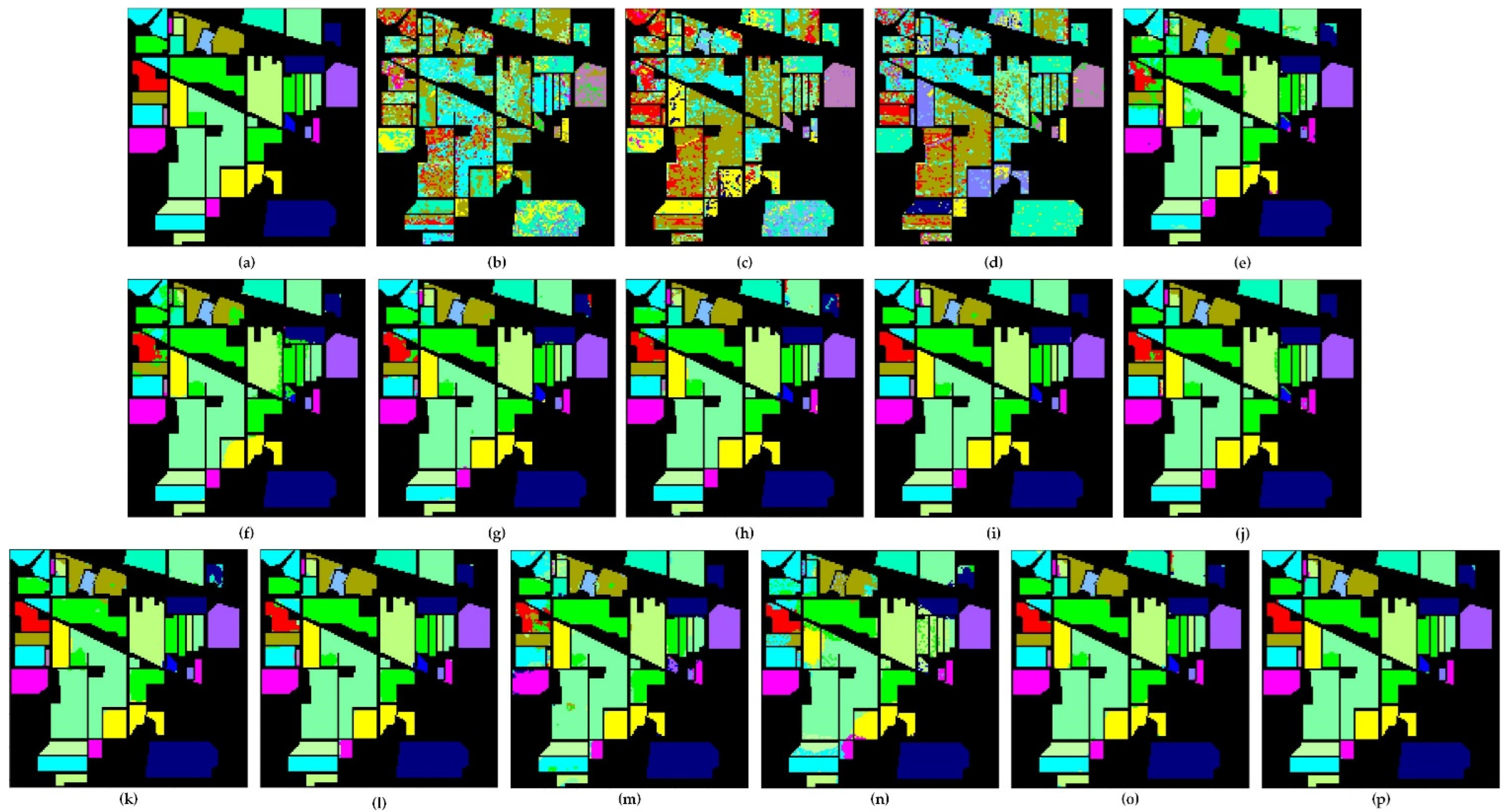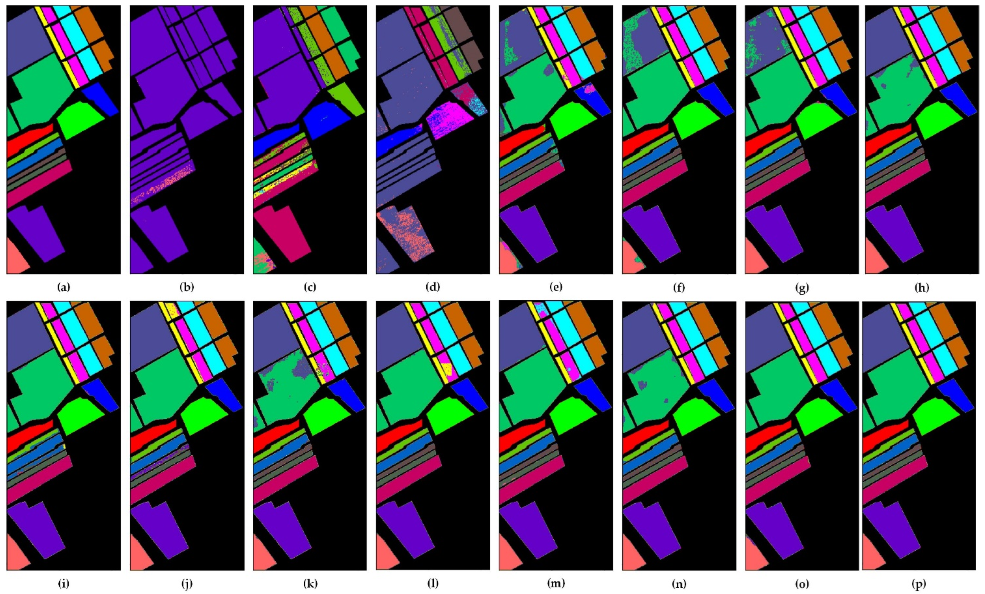Moreover, Figure 15, Figure 16, Figure 17 and Figure 18 show the classification maps of the various methods on the four datasets. Compared with other classification methods, the classification maps of the DSFNet not only have clearer edges, but also contain fewer noisy points. Our proposed method has smoother classification maps and higher classification accuracy. Because of the idiosyncratic structure of the proposed method, it can fully extract the spectral-spatial joint features of HIS, further suppress the noisy boundaries of categories, and simultaneously take advantage of the shuffle attention features from the encoder and high-level cross-connected semantic features to restore the category boundaries in the decoder phase.

3.6. Generalization Performance

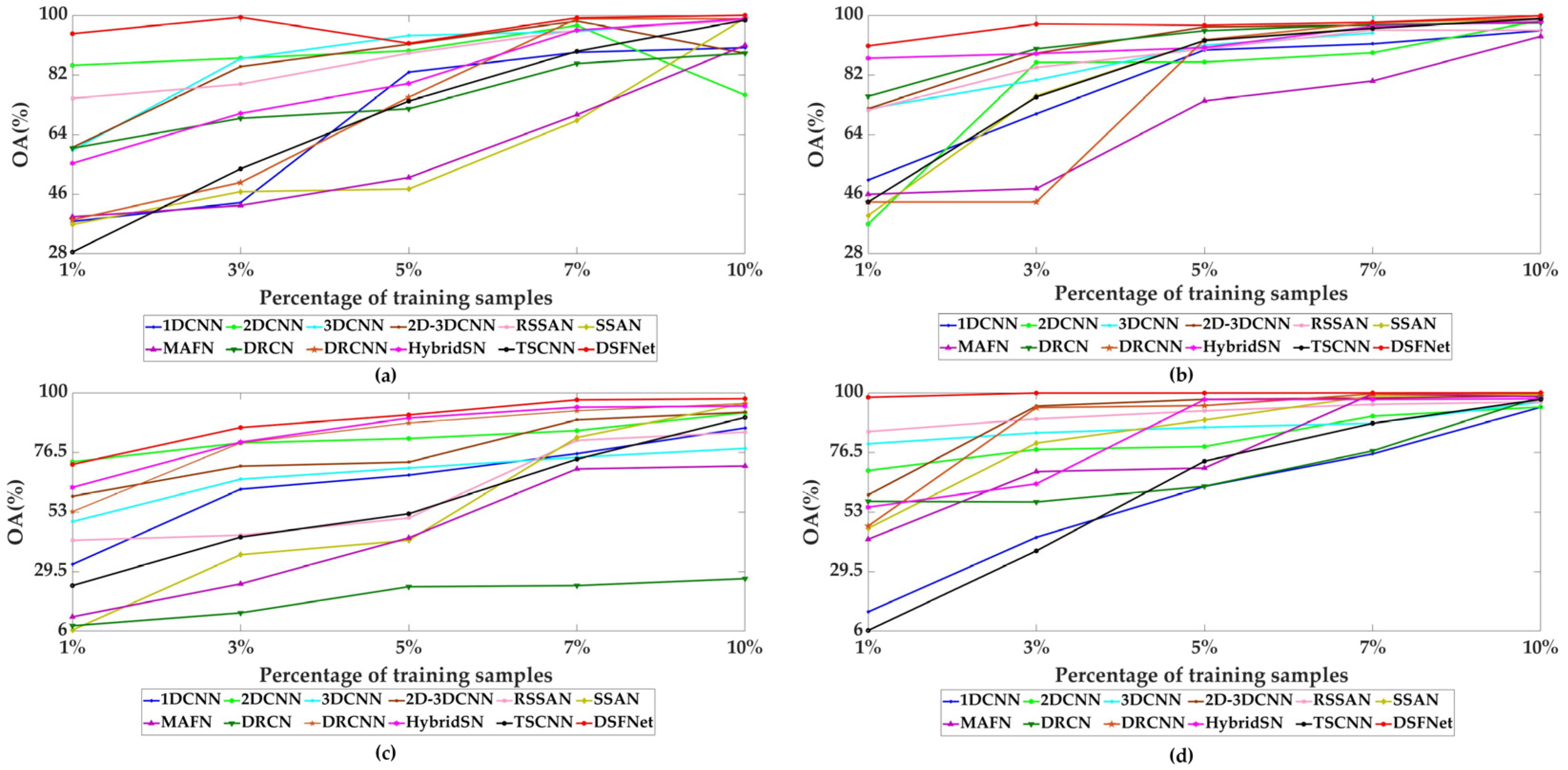
To further demonstrate the generalization performance and robustness of our proposed DSFNet under different numbers of training samples, we perform a great number of experiments among 1D_CNN, 2D_CNN, 3D_CNN, 2D_3D_CNN, RSSAN, SSAN, MAFN, DCRN, DRCNN, HybridSN, TSCNN and our DSFNet on different numbers of training samples, i.e., [1%, 3%, 5%, 7%, 10%]. Figure 19 shows the classification indication

OAs of different methods with various numbers of training samples on the SAC, UP, IP and SA datasets. As shown in Figure 19, we can clearly see that the classification performance of each method improves substantially with the increase of the number of training samples. Compared with other deep learning methods, our proposed DSFNet achieves superior classification accuracy on the four experimental datasets. For example, from Figure 19a, when the number of training samples is 1%, our method obtains 94.95% OA on the SAC dataset, which is 57.19% higher than 1D_CNN, 20.06% higher than RSSAN, and 39.05% higher than HybridSN. From Figure 19c, when the number of training samples is 10%, our method obtains 97.66% OA on the IP dataset, which is 5.54% higher than 2D_CNN, 26.53% higher than MAFN, and 7.41% higher than TSCNN. These experimental results demonstrate that our proposed DSFNet has stronger robustness and generalizability than other deep learning methods.

3.7. Ablation Experiments

3.7.1. Effectiveness Analysis of the SSAM

To fully validate the effectiveness of SSAM, ablation experiments are performed on the four HSI datasets, i.e., our proposed SSAM, eliminating channel attention (spectral-spatial), and eliminating spectral-spatial attention (channel).

Table 9. Effectiveness analysis of SSAM on the four experimental datasets.

Datasets	Schemes	Channel	Spectral-Spatial	SSAM
	Indexes
SAC	OA (%)	99.92	92.98	100
	AA (%)	99.93	86.09	100
	Kappa (%)	99.90	91.19	100
UP	OA (%)	92.97	91.62	99.89
	AA (%)	84.97	78.21	99.77
	Kappa (%)	90.65	88.87	99.85
IP	OA (%)	97.42	90.14	99.68
	AA (%)	91.81	75.22	99.44
	Kappa (%)	97.06	88.78	99.64
SA	OA (%)	96.86	94.19	99.99
	AA (%)	95.52	86.98	99.98
	Kappa (%)	96.51	93.53	99.99

The red font highlights which mechanic works best.

provide the classification results of different schemes on the four datasets, respectively. Compared with the spectral-spatial, the OA, AA and Kappa of channel are almost higher. This is because the network structure of spectral-spatial is relatively complex, and it needs more training parameters and labeled samples. From Table 9, we can explicitly see that our proposed SSAM obtains much better classification performance compared with the channel and spectral-spatial, whose evaluation indexes almost exceed 99%. Although the network structure of our proposed SSAM is more complicated, the SSAM can fully capture local and global spectral-spatial features separately and learn the interdependency of spectral and spatial information. These experimental results further prove that our proposed SSAM is beneficial for improving HSI classification performance.

3.7.2. Effectiveness Analysis of the CSFEM

The CSFEM can adequately extract global information of high-level cross-connected spectral-spatial features utilizing global average pooling and global max pooling. Different ablation structures are adopted for comparison to prove the effectiveness of the CSFEM, i.e., our proposed CSFEM, using the global average pooling (GAPM) and using the global max pooling (GMPM), as given in

Table 10. Effectiveness analysis of CSFEM on the four experimental datasets.

Datasets	Schemes	GAPM	GMPM	CSFEM
	Indexes
SAC	OA (%)	99.67	97.57	100
	AA (%)	99.55	98.23	100
	Kappa (%)	99.61	96.97	100
UP	OA (%)	95.14	98.07	99.89
	AA (%)	90.12	97.45	99.77
	Kappa (%)	93.55	97.44	99.85
IP	OA (%)	98.58	98.41	99.68
	AA (%)	98.19	95.85	99.44
	Kappa (%)	98.39	98.19	99.64
SA	OA (%)	97.63	99.02	99.99
	AA (%)	96.05	98.79	99.98
	Kappa (%)	97.36	98.91	99.99

The red font highlights which mechanic works best.

. We find that the global average pooling spectral-spatial features are as noteworthy as the global max pooling spectral-spatial features in terms of HSI classification. Although the GAPM and the GMPM achieve good classification performance, they only consider global average pooling or global max pooling spectral-spatial features and ignore the complementary relationship between them. In contrast, our proposed CSFEM employs both global average pooling and max pooling and integrates them by elementwise summation. From Table 10, it is evident that our proposed CSFEM obtains much better classification accuracy than the GAPM and GMPM. For instance, our method achieves 99.89% OA, 99.77% AA, and 99.85% Kappa on the UP dataset, which are 4.75%, 9.65% and 6.3% higher than GAPM and 1.82%, 2.32% and 2.41% higher than GMPM. This is because the average-pooled features that encode global statistics and the max-pooled features encoding the most important part can compensate for each other to capture more comprehensive and specific spectral-spatial features.

3.7.3. Effectiveness Analysis of the Proposed DSFNet

To validate the effectiveness of the SSAM, SFAM, CHSFEM and CSFEM of our proposed method, we compare the DSFNet with three other methods: using SSAM (case1), the combination of SSAM and CSFEM (case2) and the combination of SSAM, CHSFEM and SFAM (case3). The classification results of the DSFNet on the SAC dataset, UP dataset, IP dataset and SA dataset are compared with different ablation methods, as explained in

Table 11. Effectiveness analysis of the proposed DSFNet on the four experimental datasets.

Datasets	Indexes	SSAM	CHSFEM	SFAM	CSFEM	OA (%)	AA (%)	Kappa (%)
	Schemes
SAC	case1	√				94.62	94.05	93.28
	case2	√	√			98.98	99.36	98.73
	case3	√	√	√		99.75	99.68	99.69
	DSFNet	√	√	√	√	100	100	100
UP	case1	√				77.66	54.96	69.71
	case2	√	√			85.92	76.69	81.59
	case3	√	√	√		95.12	87.75	93.53
	DSFNet	√	√	√	√	99.89	99.77	99.85
IP	case1	√				84.51	60.74	82.28
	case2	√	√			87.64	70.36	85.98
	case3	√	√	√		98.44	94.01	98.22
	DSFNet	√	√	√	√	99.68	99.44	99.64
SA	case1	√				77.84	67.63	75.39
	case2	√	√			92.46	86.48	91.62
	case3	√	√	√		97.80	97.50	97.55
	DSFNet	√	√	√	√	99.99	99.98	99.99

The red font highlights which mechanic works best.

, respectively.

We introduce the CHSFEM to case2 to capture high-level spectral-spatial features. According to the Table 11, compared with case1, case2 achieves better classification accuracy. For instance, case2 obtains 77.66% OA, 54.96% AA, and 69.71% Kappa on the UP dataset, which are 22.33%, 44.81% and 30.14% higher than case1. This is because the introduced CHSFEM can not only enrich discriminative spectral-spatial multiscale features for limited labeled data but also maintain high-resolution representations throughout the process and repeatedly fuse multiscale subnet features.

We also introduce the SFAM to case3 to adaptively compress the spectral channels and introduce multiple frequency components. From Table 11, we can clearly see that case3 obtains superior classification accuracy, which demonstrate the SFAM is effective. For instance, case3 achieves 98.44% OA, 94.01% AA, and 98.22% Kappa on the IP dataset, which are 10.8%, 23.65% and 12.24% higher than case2.

The CSFEM is introduced to our proposed DSFNet to obtain the global context semantic features and restore the boundaries of categories. According to the classification results on the four hyperspectral datasets, we confirmed the effectiveness of CSFEM. For instance, our proposed DSFNet opposes 99.99% OA, 99.98% AA, and 99.99% Kappa on the SA dataset, which are 2.19%, 2.48% and 2.44% higher than case3. Our proposed method has preferable classification accuracy. This finding is owing to the unique structure of DSFNet, which makes the spectral-spatial features of HSI be fully captured.

4. Discussion and Conclusions

In this paper, we propose a discriminative spectral-spatial-semantic feature network based on shuffle and frequency attention mechanisms for HSI classification, which consists of an encoder and a decoder. In the encoder and decoder stages, the SSAMs and SFAMs can capture richer and more multifarious joint spectral-spatial features, and further improve the expression of features. The high-level context-aware multiscale spectral-spatial features are extracted by the CHSFEM, which are scale-invariant and solve the problem that deep networks cannot extract features of small-sized samples. The CSFEMs can suppress noisy boundaries with similar topographic structures and utilize the utmost out of the spectral-spatial shuffle attention features from the encoder to better guide the high-level spectral-spatial attention features to restore category boundaries in the decoder part. Finally, we also introduce dropout and BN optimization methods to boost the classification accuracy.

The classification performance of our proposed DSFNet is affected by five vital parameters. To obtain the best classification results, we discuss the influences of these five framework parameters on HSI classification when setting different values. Moreover, to prove the superiority of our proposed DSFNet, lots of comparison experiments including three traditional classification methods and eleven classification methods based on deep learning are conducted on four common datasets. The evaluation indexes of OA, AA and Kappa on four datasets all exceed 99%. Meanwhile, by comparing with the diverse classification methods, we analyze the advantages of our proposed method from four different perspectives. In addition, the above ablation experiments also adequately demonstrate the effectiveness of SSAM, CHSFEM, SFAM and CSFEM.

HSI classification methods have achieved satisfactory results, but they often need numerous training parameters, longer training time and enormous computational cost. Therefore, our feature research direction will focus on how to reduce the computational. In addition, HSI classification has been widely used in many computer fields. In the future, we will also try to apply the proposed method to some computer vision tasks, such as tumor recognition.