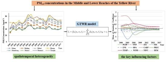
Identifying Spatiotemporal Heterogeneity of PM_2.5 Concentrations and the Key Influencing Factors in the Middle and Lower Reaches of the Yellow River

Abstract

Fine particulate matter (PM_2.5) is a harmful air pollutant that seriously affects public health and sustainable urban development. Previous studies analyzed the spatial pattern and driving factors of PM_2.5 concentrations in different regions. However, the spatiotemporal heterogeneity of various influencing factors on PM_2.5 was ignored. This study applies the geographically and temporally weighted regression (GTWR) model and geographic information system (GIS) analysis methods to investigate the spatiotemporal heterogeneity of PM_2.5 concentrations and the influencing factors in the middle and lower reaches of the Yellow River from 2000 to 2017. The findings indicate that: (1) the annual average of PM_2.5 concentrations in the middle and lower reaches of the Yellow River show an overall trend of first rising and then decreasing from 2000 to 2017. In addition, there are significant differences in inter-province PM_2.5 pollution in the study area, the PM_2.5 concentrations of Tianjin City, Shandong Province, and Henan Province were far higher than the overall mean value of the study area. (2) PM_2.5 concentrations in western cities showed a declining trend, while it had a gradually rising trend in the middle and eastern cities of the study area. Meanwhile, the PM_2.5 pollution showed the characteristics of path dependence and region locking. (3) the PM_2.5 concentrations had significant spatial agglomeration characteristics from 2000 to 2017. The “High-High (H-H)” clusters were mainly concentrated in the southern Hebei Province and the northern Henan Province, and the “Low-Low (L-L)” clusters were concentrated in northwest marginal cities in the study area. (4) The influencing factors of PM_2.5 have significant spatiotemporal non-stationary characteristics, and there are obvious differences in the direction and intensity of socio-economic and natural factors. Overall, the variable of temperature is one of the most important natural conditions to play a positive impact on PM_2.5, while elevation makes a strong negative impact on PM_2.5. Car ownership and population density are the main socio-economic influencing factors which make a positive effect on PM_2.5, while the variable of foreign direct investment (FDI) plays a strong negative effect on PM_2.5. The results of this study are useful for understanding the spatiotemporal distribution characteristics of PM_2.5 concentrations and formulating policies to alleviate haze pollution by policymakers in the Yellow River Basin.

1. Introduction

With rapid urbanization and industrialization in recent years, high concentrations of PM_2.5 (Fine particles with a diameter ≤2.5 µm) are one of the main causes of air pollution, which has become the most urgent and prominent environmental problem in China [1,2]. Some existing research on air pollution showed that PM_2.5 exposure generates not only respiratory and cardiovascular diseases and threatens the physical and mental health of residents seriously [3,4] but also hinders economic growth and social stability. Recent studies showed that PM_2.5 pollution is relevant to about 1.2 million people premature deaths per year between 1999 and 2010 [5]. In China, about 40% of premature deaths are associated with air pollution [6]. Consequently, in order to deal with the problem of poor air pollution, the Chinese government has introduced a series of strict measures to improve air quality [7,8]. As an important ecological security barrier in China, the Yellow River Basin plays a significant role in air pollution management in China. However, this region, especially the middle and lower reaches, has experienced serious air pollution due to drastic population activities and economic development in recent years [9,10]. It is urgent to study the spatial and temporal characteristics to influence factors of PM_2.5 pollution and to provide a scientific basis for PM_2.5 pollution governance in the middle and lower reaches of the Yellow River Basin.

The existing literature on PM_2.5 pollution is mainly carried out from the aspects of spatiotemporal distribution, influencing factors, and research methods [11,12,13]. In terms of the spatiotemporal pattern of PM_2.5 concentrations, previous researchers examined the spatiotemporal distribution of PM_2.5 concentrations at different spatial scales, such as the national scales [14], the provincial scales [15,16], or the urban agglomerations scales [17,18]. Based on the analysis results of different spatial scales, numerous research found that the distribution of PM_2.5 concentrations had significant spatial differentiation characteristics. However, few previous studies paid attention to PM_2.5 pollution in the middle and lower reaches of the Yellow River Basin, which constitutes an important part of China’s economic development and environmental protection.

On the surface, PM_2.5 pollution comes from meteorological factors, while actual emissions always are human activities, including automobile exhaust and industrial waste gas, etc. [19,20,21]. Therefore, its influencing factors are multifaceted and complex. From the perspective of the impacts of human activities, existing studies mainly focus on social and economic development [22,23], population distribution [24], traffic emission [25], industrial structure [26], land-use changes [27], and natural conditions [28,29]. For example, some scholars pointed out that urbanization had a positive impact on the increase in PM_2.5 concentrations by studying the relationship between PM_2.5 concentrations and urbanization in China [30,31]. Other studies found that cities with high population density and heavy traffic had higher concentrations of PM_2.5 [32]. There are also previous studies confirming that regional natural conditions such as wind speed, annual precipitation, and temperature are the main influencing factors of PM_2.5 concentrations [33,34]. Briefly, the factors that impact PM_2.5 concentrations involve socio-economic and natural conditions. However, most previous studies concentrated separately on either natural conditions or socio-economic factors. The PM_2.5 concentrations in any area are the result of the interaction between nature and human activities [35]. Obviously, using only a single perspective may lead to inaccurate analysis results, so it is necessary to consider the comprehensive influence of both natural and socio-economic conditions on PM_2.5 into account together.

Various research methods were used to investigate the influencing factors of PM_2.5 concentrations, such as the linear regression model [36] and econometric models [37,38]. Some researchers analyzed the factors for the PM_2.5 distribution in China by applying the nonparametric additive regression model [39]. In fact, the spatial distribution of different influencing factors is heterogeneous, and the influencing factors of different geographical locations have different effects on PM_2.5, so the analysis results of traditional econometric models were always biased because the spatial effects of factors were neglected [40]. Gradually, spatial statistical models were utilized in the investigation of PM_2.5 pollution driving factors. Based on the spatial Durbin model, spatial lag model (SLM), and spatial error model (SEM), some studies used these methods to investigate the spatial spillover effects of PM_2.5 and its influencing factors [41,42,43].

In addition, the geographically weighted regression (GWR) model that considers spatial non-stationarity features was conducted to analyze the relationship between PM_2.5 and driving factors. Wang et al. [44] used the GWR model to detect the spatial heterogeneity of the influencing factors of PM_2.5 concentrations in Chinese cities and found that there were significant differences in the intensity of spatial heterogeneity. Compared with the GWR model, which can only treat spatial variations in multivariate data, the Geographically and temporally weighted regression (GTWR) model, which integrates spatial and temporal variations in PM_2.5 and influencing factors relationship, gained more and more attention in the current research [45,46]. These documents are helpful in accurately understanding the causes of PM_2.5 and promoting its governance.

Although more and more literature studies the spatiotemporal characteristics of PM_2.5 and its influencing factors by applying spatial statistical models, few studies comprehensively utilized spatial autocorrelation analysis and the GTWR model to explore the characteristics of PM_2.5 and its driving factors in river regions. In addition, most of the previous studies only focus on the spatial difference of the influencing factors, then the temporal variation effects of factors are ignored. Therefore, the GTWR model is more accurate and effective by considering the non-stationarity of spatial and temporal dimensions [47]. This study aims to investigate the spatial-temporal dynamics of PM_2.5 concentrations and explore its influencing factors from two aspects of natural and socio-economic conditions by using the GTWR model. The main contributions of this study are summarized as follows: (1) the spatiotemporal characteristic of PM_2.5 concentrations was analyzed in the middle and lower reaches of the Yellow River Basin from 2000 to 2017; (2) the spatial agglomeration features of PM_2.5 was investigated based on spatial autocorrelation model; (3) the spatiotemporal heterogeneity of natural and socio-economic factors influencing PM_2.5 were examined by applying GTWR model. The results of this study can enrich the content of PM_2.5 distribution in the watershed. Meanwhile, they also provide reference evidence for PM_2.5 control policies in the middle and lower reaches of the Yellow River Basin.

The above-mentioned research rarely starts from the perspective of the river basin, especially the Yellow River basin. Since the ecological protection and high-quality development of the Yellow River basin became a national strategy in 2019, the improvement of the atmospheric environment in the Yellow River basin has become an urgent task, and the problem of air pollution in the middle and lower reaches of the Yellow River is particularly acute; therefore, it is more important to explore the spatial distribution difference and the spatial and temporal heterogeneity of the influencing factors, to carry out regional governance and regional joint defense linkage. Spatiotemporal geographical weighting models were originally used to detect spatiotemporal variations in factors affecting house prices, and then the GTWR model is verified and compared with other models, respectively, and the kernel function selection method and non-stationary test method are defined to verify the effectiveness of the method. It was proved that the GTWR model is significantly higher than the goodness of fit of the ordinary least squares (OLS) model and GWR model and is more reliable [48,49,50].

This paper selects the middle and lower reaches of the Yellow River with high pollution as the research area and uses the geographically and temporally weighted model to explore the impact intensity of five natural environmental factors and seven socio-economic indicators on PM_2.5 pollution from two scales of time and space and their interaction. In the environment of environmental protection, the research results of this paper are of great significance for pollution prevention and control as well as refined and differentiated governance.

2. Material and Data Sources

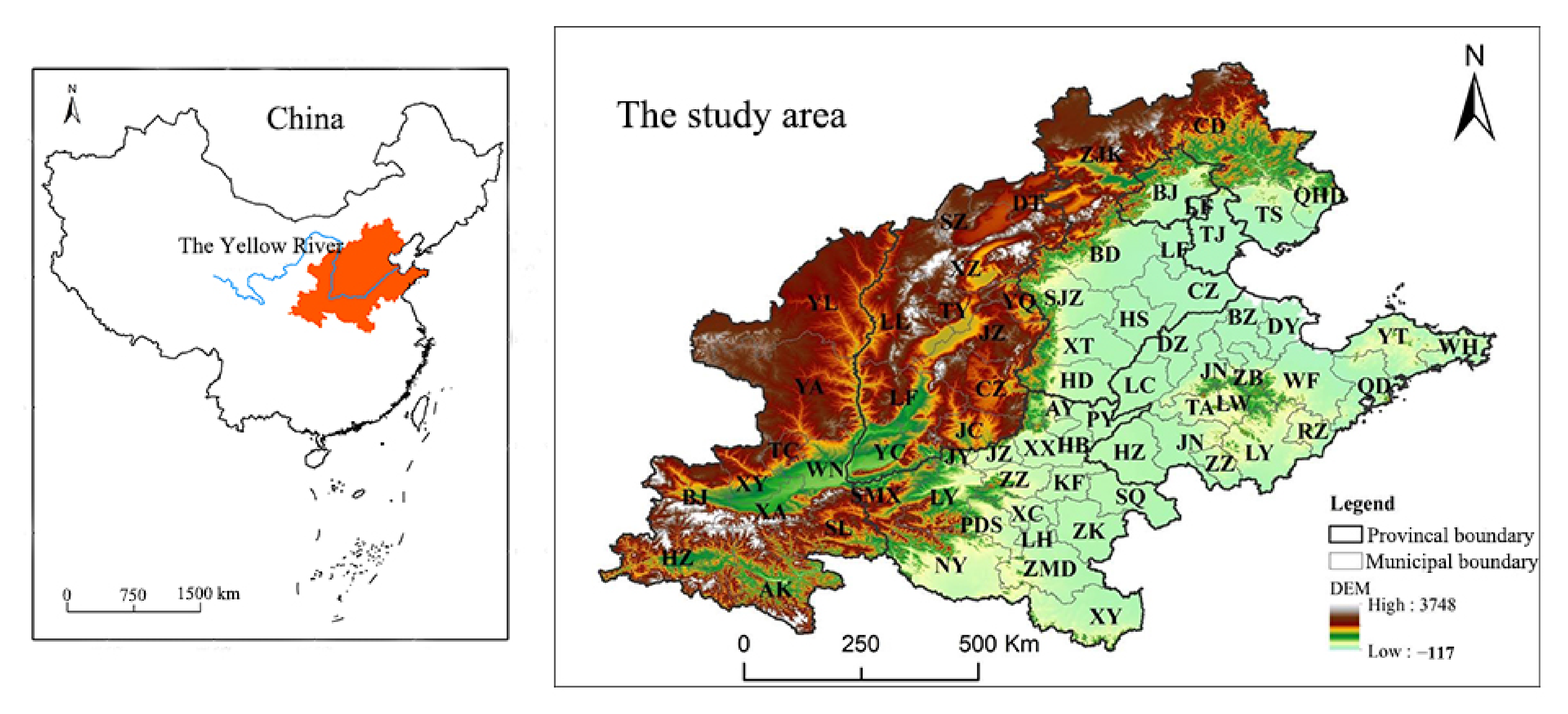
2.1. Study Area

In recent years, the improvement of the air quality in China has become an urgent task, and the problem of PM_2.5 pollution in the middle and lower reaches of the Yellow River is particularly acute. Based on the current situation of PM_2.5 concentrations in the middle and lower reaches of the Yellow River, the scope of the study area was expanded to the Loess Plateau and the Huang-Huai-Hai Plain (Figure 1). There are 67 prefecture-level cities located in five provinces (17 prefecture-level cities located in Shandong Province, 18 prefecture-level cities located in Henan Province, 10 prefecture-level cities located in Shaanxi Province, 11 prefecture-level cities located in Shanxi Province, and 11 prefecture-level cities located in Hebei Province), and includes two municipalities (Beijing and Tianjin). In this paper, the spatiotemporal variation characteristics of PM_2.5 concentrations were discussed at the urban scale, and the main influencing factors were revealed from the dimensions of socio-economic factors and natural conditions.

2.2. Data Sources and Preprocessing

2.2.1. PM_2.5 Concentrations Data

PM_2.5 concentrations data are derived from the Atmospheric Composition Analysis Group at Washington University in St. Louis (https://sites.wustl.edu/acag/datasets/surface-pm2-5/, accessed on 10 April 2022), which provides a published global dataset of PM_2.5 concentrations. This dataset has a high spatial resolution (the raw data 0.1° × 0.1°), good accuracy with a cross-validated R² of 0.81 [51], and has been widely applied in many previous studies [52,53]. In this study, the regional statistical tool ArcGIS was used to extract the annual average value of PM_2.5 concentrations in the middle and lower reaches of the Yellow River from 2000 to 2017. According to the Ambient Air Quality Standard of China (GB3095-2012) and the related literature [8,54,55], PM_2.5 concentrations were divided into seven categories as follows: ultra-low concentrations (<15 µg/m³), lower concentrations (15–25 µg/m³), low concentrations (25–35 µg/m³), medium concentrations (35–50 µg/m³), high concentrations (50–70 µg/m³), higher concentrations (70–100 µg/m³), ultra-high concentrations (>100 µg/m³).

2.2.2. Socio-Economic Data

As shown in the above existing literature, socio-economic factors are an important part of PM_2.5 pollution [22]. Previous studies confirmed that GDP, population density, industrial structure, and other human activity factors have a certain impact on air pollution [24,26]. Based on the socio-economic situation of the middle and lower reaches of the Yellow River Basin, the effect of human activities and economic development on PM_2.5 concentrations were investigated using seven socio-economic indicators, including GDP per capita (PGDP), population density (POP), the proportion of secondary industry (SEC), foreign direct investment (FDI), proportion of built-up area (BPA), car ownership per 10,000 people (CARP), and energy consumption index (ENE). These socio-economic data were mainly from China City Statistical Yearbook (2001–2018) and the provincial statistical yearbook on the China National Knowledge Infrastructure (CNKI: http://www.cnki.net/, accessed on 20 April 2020) to obtain prefecture-level city data. In order to ensure continuity of socio-economic data, the interpolation method was adopted for calculating a small number of missing values in some years (Figure 2).

2.2.3. Natural Conditions Data

Given that the natural factors, including climate and environment, were associated with aspects of diffusion and secondary influences of PM_2.5 pollution [33,34], based on the climate conditions and environmental characteristics of the middle and lower reaches of the Yellow River Basin, five natural factors were selected to explore the impact on PM_2.5 in this study (Figure 3), including temperature (TEMP), precipitation (PREC), wind speed (WIND), Normalized Difference Vegetation Index (NDVI), and Digital Elevation Model (DEM). Among them, The NDVI is a commonly applied factor in analyzing the impact of green vegetation on air pollution and has a certain correlation with PM_2.5. Meteorological data (including temperature, precipitation, and wind speed) are obtained from the National Tibetan Plateau/Third Pole Environment Data Center (https://data.tpdc.ac.cn, accessed on 30 April 2022). This dataset has high spatial resolution and long time series, and its accuracy is better than the international reanalysis data [56,57]. The NDVI and DEM data are derived from the Resources and Environment Science and Data Center of the Chinese Academy of Science (https://www.resdc.cn/DOI/doi.aspx?DOIid=49, accessed on 30 April 2022).

3. Methodology

3.1. Spatial Autocorrelation Models

3.1.1. Global Spatial Autocorrelation Analysis

Global spatial autocorrelation analysis is mainly used to measure the spatial correlation degree of PM_2.5 and analyze the spatial distribution feature in adjacent locations of PM_2.5 overall, to judge whether PM_2.5 concentrations have spatial aggregation [58]. The global spatial autocorrelation is represented by Moran’s I index, and the calculation formula is as follows:

$$Moran\prime s^{} I=\frac{{\displaystyle \sum _{i=1}^n{\displaystyle \sum _{j=1}^n{W}_{ij}(X_i-\overline{X})(X_j-\overline{X})}}}{s^2{\displaystyle \sum _{i=1}^n{\displaystyle \sum _{j=1}^n{W}_{ij}}}}$$

(1)

where n is the number of research units (prefecture-level cities), $X_i$ and $X_j$ are the average annual concentrations of PM_2.5 in city $i$ and city $j$, $\overline{X}$ is the average annual concentrations of PM_2.5 in all cities, and $W_{ij}$ is the space weight matrix. The value range of Moran’s I is generally [−1, 1]. $0<I\le 1$ means there is a positive spatial correlation between regions, while $-1\le I<0$ means there is a negative spatial correlation between regions, $I=0$ indicates that the spatial data are randomly distributed or do not have a spatial correlation. The Z score can be used to test the correlation between the values:

$$Z(I)=\frac{I-E(I)}{\sqrt{Var(I)}}$$

(2)

$E(I)$ and $Var(I)$ are the value of mathematical expectation and the variance. The significance level is 0.05.

3.1.2. Local Spatial Autocorrelation Analysis

Anselin pointed out that Global spatial autocorrelation analysis can only reflect the overall distribution characteristics [59] but cannot calculate and analyze the local differences of spatial objects. Therefore, it is necessary to further explore the spatial aggregation and dispersion between the local unit and its neighboring units. The local spatial autocorrelation model can be calculated as follows:

$$Local Moran\prime s I_i=\frac{n(X_i-\overline{X}){\displaystyle {\sum }_{j=1}^m{W}_{ij}(X_j-\overline{X})}}{{{\displaystyle {\sum }_{j=1}^n(X_j-\overline{X})}}^2}$$

(3)

$$S^2=\frac{1}{n}{\displaystyle \sum _{i=1}^n{(X_i-\overline{X})}^2}$$

(4)

In the Formula (3), n represents the number of prefecture-level cities, X_i and X_j represent the average annual concentrations of PM_2.5 in cities i and j. $\overline{X}$ is the average annual concentrations in all cities and $W_{ij}$ is the spatial weight matrix. m represents the number of cities that are adjacent to city i. The Z score for the standardized statistics are as follows:

$$Z(I_i)=\frac{|1-E\left(I_i\right)|}{\sqrt{Var(I_i)}}$$

(5)

The local spatial autocorrelation can be classified into four types: (1) High–High (H-H) type represents that the high PM_2.5 value area is adjacent to the high PM_2.5 value area; (2) High–Low (H-L) type represents that the high PM_2.5 value area is adjacent to the low PM_2.5 value area; (3) Low–High (L-H)type represents that the low PM_2.5 value area is adjacent to the high PM_2.5 value area; (4) Low–Low (L-L) type represents that the low PM_2.5 value area is adjacent to the low PM_2.5 value area.

3.1.3. Geographically and Temporally Weighted Regression Model

Compared with the traditional linear regression model, such as the ordinary least squares (OLS) model, the geographically weighted regression model (GWR) quantifies spatial heterogeneity of variables by calculating locally weighted regression for location [60]. Since the GWR model only pays attention to spatial heterogeneity and ignores the changes caused by temporal dimensions, the GTWR model was established by Huang et al. [47] and further introduced the temporal dimension based on the GWR model. GTWR model can better reveal the spatial and temporal heterogeneity and detect non-stationary spatiotemporal characteristics of explanatory variables. In this study, the GTWR model can be calculated as follows:

$$Y_i={\beta }_0\left({\mu }_i,{\upsilon }_i,t_i\right)+{\displaystyle \sum _{k=1}^n{\beta }_k\left({\mu }_i,{\upsilon }_i,t_i\right)}{x}_{ik}+{\epsilon }_i$$

(6)

In the Formula (6), $Y_i$ denotes the average annual value of PM_2.5 concentrations of the city i, t denotes the year studied, $x_{ik}$(k = 1,2,…, m) denotes the value of the explanatory variable k of the city i; $\left({\mu }_i,{\upsilon }_i,t_i\right)$ is the space-time dimension of the city i; ${\mu }_i$ and ${\upsilon }_i$ denote the longitude and latitude of the city i, $t_i$ denotes the time coordinates of the city i; ${\beta }_0\left({\mu }_i,{\upsilon }_i,t_i\right)$ denotes the intercept value, ${\beta }_k\left({\mu }_i,{\upsilon }_i,t_i\right)$ (k = 1,2,…, m) denotes the regression coefficient and ${\epsilon }_i$ is the error term for city i representing the difference between the observed value and estimated value

The essential question of the GTWR model is to estimate ${\beta }_k\left({\mu }_i,{\upsilon }_i,t_i\right)$, and the estimation equation can be calculated as follows:

$$\stackrel{⌢}{\beta }\left({\mu }_i,{\upsilon }_i,t_i\right)=[X^{T}W({\mu }_i,{\upsilon }_i,t_i{)X]}^{-1}{X}^{T}W({\mu }_i,{\upsilon }_i,t_i)Y$$

(7)

In Formula (7), $W({\mu }_i,{\upsilon }_i,t_i)=\mathrm{diag}({\alpha }_{i1},{\alpha }_{i2},\dots ,{\alpha }_{in})$, n denotes the number of cities. The diagonal elements ${\alpha }_{ij}(1\le j\le n)$ denote space–time distance functions of $(\mu ,\upsilon ,t)$ corresponding to the weights when calibrating a weighted regression near city i, and X denotes a vector expressing the parameters.

4. Results and Discussion

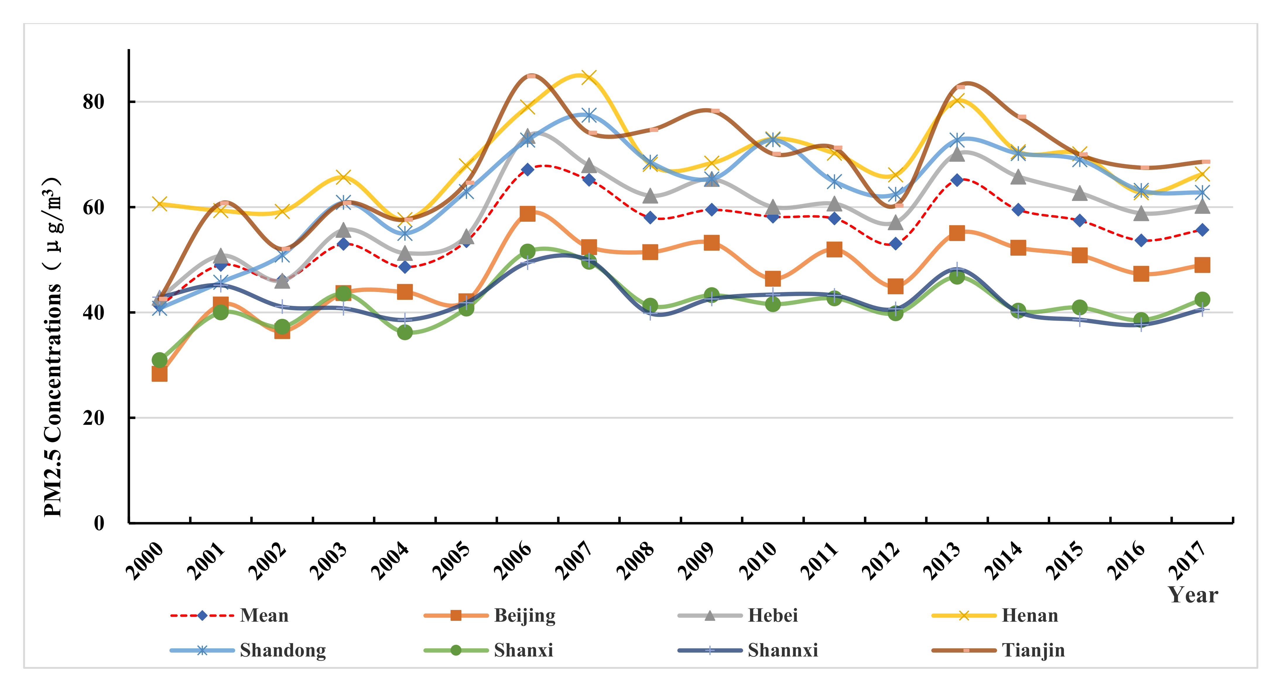
4.1. Temporal Variation Characteristics of PM_2.5 Concentrations

The proportion of 69 cities with different PM_2.5 concentrations grades was used to reflect the trend of temporal variation from 2000 to 2017 (Figure 4). the annual average PM_2.5 concentrations in the middle and lower reaches of the Yellow River showed an overall trend of increasing first and then decreasing. The annual average PM_2.5 concentrations increased significantly from 41.28 µg/m³ to 67.12 µg/m³ from 2000 to 2006; then, the value decreased from 67.12 µg/m³ to 55.69 µg/m³ from 2006 to 2017 (

Table 1. The annual average PM_2.5 concentrations of the study area (unit: μg/m³).

Year	2000	2003	2006	2009	2012	2015	2017
Average of the whole study area	41.28	53.00	67.12	59.48	53.06	57.45	55.69
Beijing Municipality	28.37	43.66	58.73	53.25	44.97	50.85	48.98
Hebei Province	42.81	55.66	73.52	65.32	57.11	62.69	60.21
Henan Province	60.60	65.65	78.99	68.35	66.12	70.10	66.26
Shandong Province	40.78	60.88	72.75	65.34	62.45	68.99	62.77
Shanxi Province	30.94	43.57	51.54	43.27	39.84	40.94	42.45
Shannxi Province	42.90	40.77	49.46	42.57	40.66	38.62	40.59
Tianjin Municipality	42.54	60.78	84.83	78.29	60.28	69.97	68.59

). In terms of the proportion of each PM_2.5 concentration grade, the ultra-high regions where the annual average PM_2.5 concentration is higher than 100 µg/m³ appeared in 2006, 2007, and 2013, respectively. Overall, the PM_2.5 pollution was still very serious. The annual average of PM_2.5 in 2017 (55.69 µg/m³) was higher than its value in 2000 (41.28 µg/m³); this indicates that it is a very urgent problem to improve the air quality through effective governance.

In order to better investigate the regional variations in PM_2.5 concentrations in the study area, the five provinces and two municipalities with an annual average of PM_2.5 were analyzed from 2000 to 2017 (Figure 5). It was found that, although the increase in annual average PM_2.5 concentrations is fluctuant during the study period, there are still obvious differences between five provinces and two municipalities (Figure 5).

The annual average PM_2.5 concentrations of Tianjin, Shandong Province, and Henan Province has been far higher than the overall mean value in the middle and lower reaches of the Yellow River from 2000 to 2017. The annual average PM_2.5 concentrations of Tianjin increased significantly from 42.54 µg/m³ (2000) to 68.59 µg/m³ (2017). The variation trends of Hebei Province were basically consistent with the overall variation trend of the study area. Different from other provinces, the annual average of PM_2.5 concentrations in Shaanxi Province decreased in a fluctuation way from 42.90 µg/m³ (2000) to 40.59 µg/m³ (2017). This shows that the pollution degree of PM_2.5 concentrations in the study area was obviously different from 2000 to 2017.

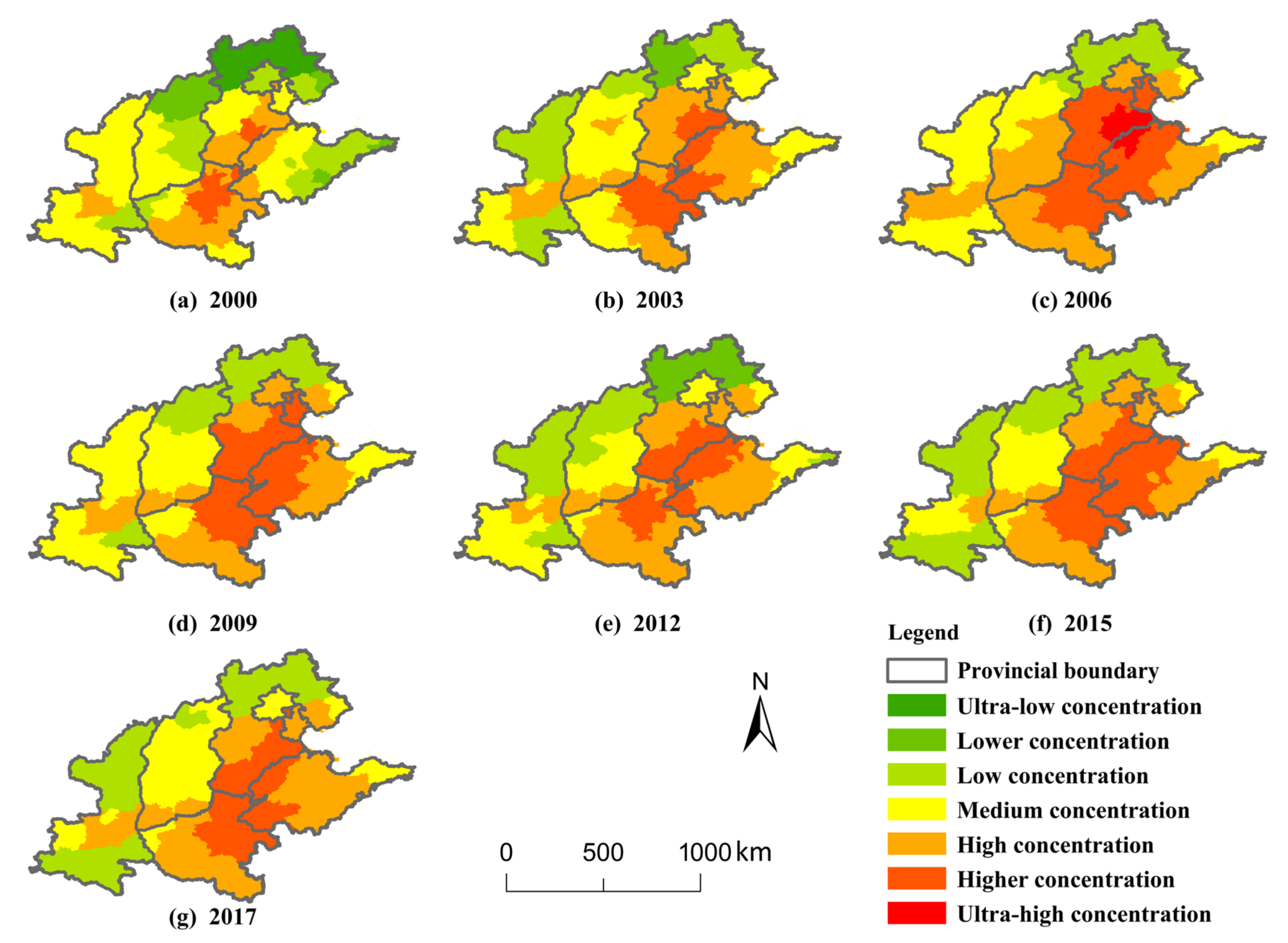
4.2. Spatial Distribution Characteristics of PM_2.5 Concentrations

The spatial evolution feature of annual average PM_2.5 concentrations in the middle and lower reaches of the Yellow River was investigated by using GIS spatial analysis methods from 2000 to 2017 (Figure 6). Overall, the PM_2.5 pollution exhibited obvious spatial differentiation features. The annual average of PM_2.5 in western cities showed a declining trend, while it had a gradually rising trend in middle and eastern cities of the study area. Specifically, in 2006, the values of eastern cities, such as Cangzhou City, Hengshui Ctiy, and Dezhou City, were significantly higher than that of the surrounding areas. Because these cities are important energy bases in China, the industrial structure dominated by the petrochemical industry increases the possibility of PM_2.5 pollution. The extensive economic development mode dominated by resources made these cities face serious air quality problems. The PM_2.5 concentrations of eastern cities increased from north to south, and the cities in the north part of the study area had undergone a decrease during the study period. However, most middle and eastern cities had experienced an increase at first and then a decrease from 2000 to 2017. It is noteworthy that the PM_2.5 pollution showed the characteristics of path dependence and region locking. Cities with high PM_2.5 values are always located in northern Henan Province, western Shandong Province, and southern Hebei Province. It shows that these cities are facing serious air pollution challenges and control pressures.

4.3. Spatial Autocorrelation Analysis of PM_2.5 Concentrations

4.3.1. Global Spatial Autocorrelation Features

The global spatial autocorrelation results (Moran’s I index) were calculated based on the annual average PM_2.5 concentrations on the prefecture-level city scale from 2000 to 2017 (

Table 2. Results of Global spatial autocorrelation Moran’s I index from 2000 to 2017.

Year	Moran’s I	Z-Score	p-Value	Year	Moran’s I	Z-Score	p-Value
2000	0.71	8.61	0.00	2009	0.71	8.55	0.00
2001	0.63	7.62	0.00	2010	0.76	9.12	0.00
2002	0.63	7.63	0.00	2011	0.70	8.38	0.00
2003	0.68	8.17	0.00	2012	0.73	8.77	0.00
2004	0.65	7.90	0.00	2013	0.72	8.64	0.00
2005	0.71	8.55	0.00	2014	0.74	8.85	0.00
2006	0.67	8.14	0.00	2015	0.75	8.99	0.00
2007	0.73	8.80	0.00	2016	0.71	8.57	0.00
2008	0.72	8.69	0.00	2017	0.72	8.61	0.00

). All the values of global Moran’s I were >0.6, and the p-value was 0.00, indicating that the 1% significance level test passed (Z = 1.96). This suggests that the spatial distribution of PM_2.5 concentrations has a positive spatial correlation in the study area, and the spatial agglomeration phenomenon is obvious. It can be proved that urban PM_2.5 concentrations in the study area were impacted not only by their own emission but also by surrounding cities. The variation in Moran’s I first presented a fluctuating rise trend, increasing from 0.63 to 0.76 from 2001 to 2010, followed by a decrease to 0.72 in 2017. These results indicated that the spatial correlation of PM_2.5 concentrations between cities was still strong in the study area.

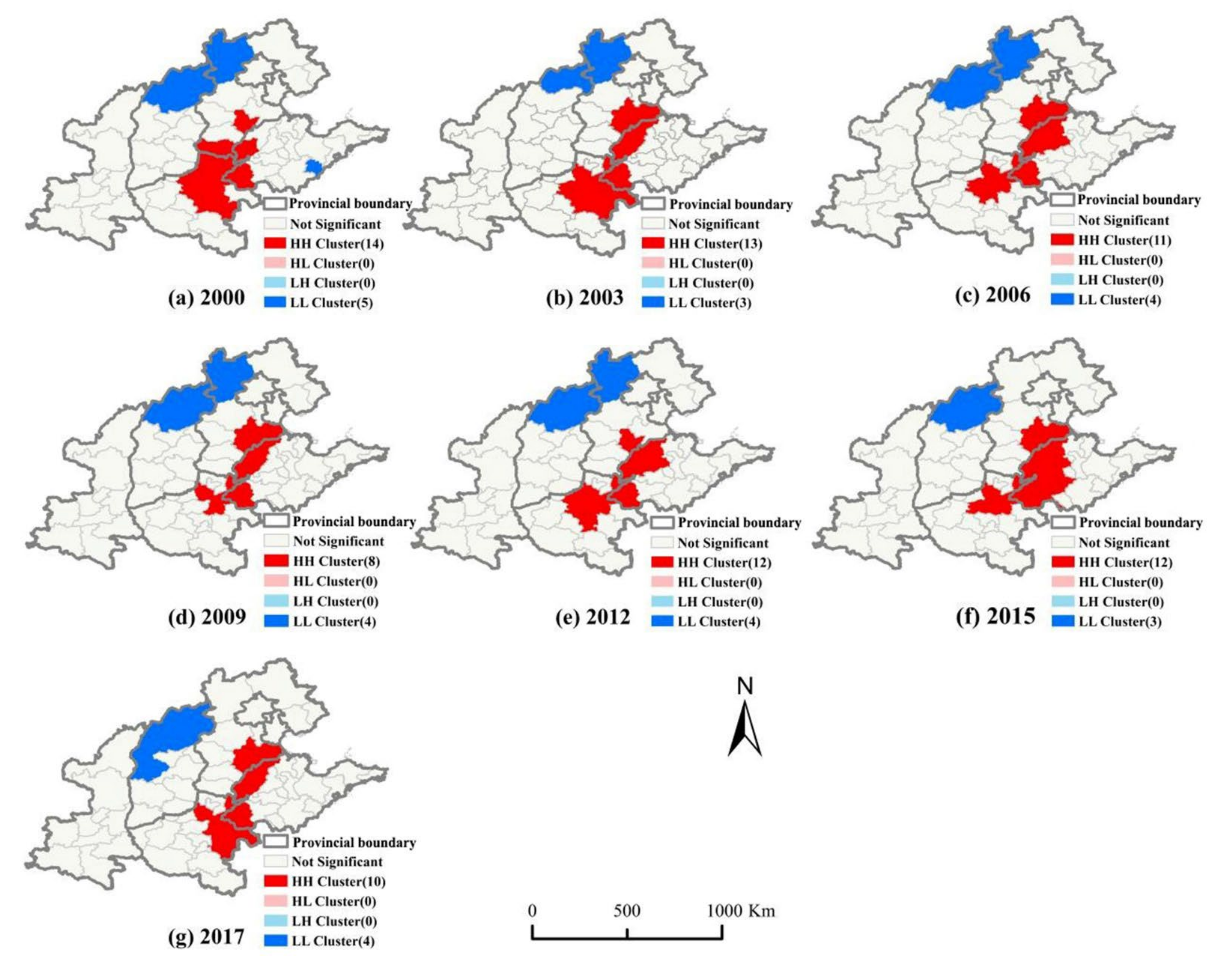
4.3.2. Local Spatial Autocorrelation Features

Based on the results of local spatial autocorrelation analysis, the local agglomeration maps were drawn in ArcGIS 10.2 software (Redlands, CA, USA) (Figure 7). The High–High (H-H) clusters were concentrated in the southern Hebei Province and the northern Henan Province. The number of cities with H-H types changed from 14 to 10 from 2000 to 2017, indicating a fluctuating downward trend. Regarding these cities with high PM_2.5 values (

Table 3. Local spatial autocorrelation statistics of cities in study area.

Types	Number of Cities (Units)
	2000	2003	2006	2009	2012	2015	2017
HH	14	13	11	8	12	12	10
LL	5	3	4	4	4	3	4

), it is necessary to take regional joint control measures to deal with air pollution on an urban scale. The Low–Low (L-L) clusters were concentrated in northwest marginal cities in the study area, such as northern Shanxi Province and northwestern Hebei Province. The number of cities with L-L types changed from five to four between 2000 and 2017. Other types, including High–Low (H-L) clusters and Low–High (L-H) clusters, had not been seen in the study area during the study period, mainly because PM_2.5 has strong spatial dispersion, and it is difficult to have independent areas with high or low value. These results demonstrated that the PM_2.5 concentrations had an obvious local spatial autocorrelation feature.

4.4. Determination of the Best Model

In this study, seven socio-economic factors and five natural conditions were selected as explanatory variables to construct an index system. The multicollinearity test was carried out on all indicators, and the results showed that the variance inflation factor of all indicators was less than 7.5, indicating no multicollinearity. Therefore, the influencing factors of PM_2.5 concentrations in the study area can be analyzed by using quantitative regression models.

According to the data characteristics, OLS, GWR, temporally weighted regression (TWR), and GTWR models were analyzed, respectively, and the performance of the four models was compared through R²-adjusted (

Table 4. Comparison of regression results of OLS, GWR, TWR, and GTWR model.

Model	R2	R2-Adjusted	AICc	Residual Squares
OLS	0.692246	0.684388	−753.33726	5.5991
TWR	0.803587	0.798573	−881.816	3.58083
GWR	0.878789	0.875694	−997.256	2.20983
GTWR	0.953621	0.952437	−1149.7	0.845549

). The results showed that the R²-adjusted increased from 0.684 (OLS model), 0.798 (TWR model), and 0.875 (GWR model) to 0.952 (GTWR model). The magnitude of the residuals squared is also OLS (5.599) > TWR (3.580) > GWR (2.209) > GTWR (0.845). Compared with the other three models, the explanatory power of the GTWR model is significantly improved, and considering the spatiotemporal heterogeneity at the same time, it can better reflect the influence degree of each factor on PM_2.5 concentrations.

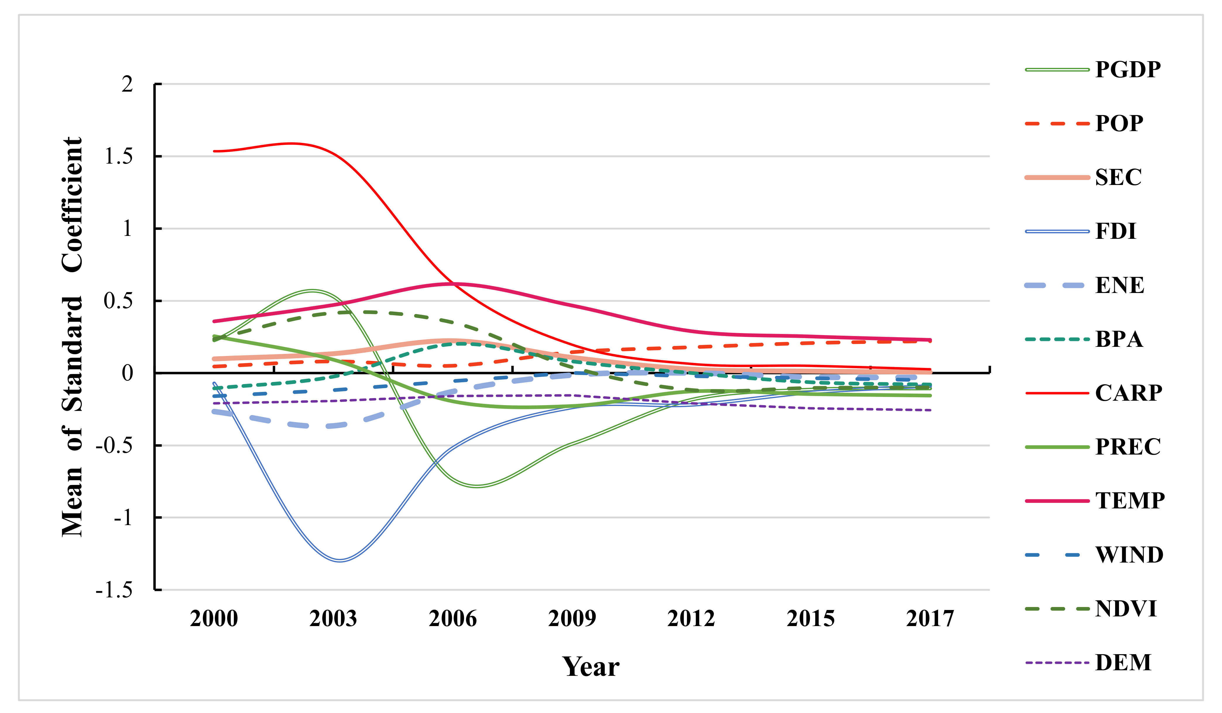
4.5. The Temporal and Spatial Variation in the Standard Coefficients of Explanatory Variables in GTWR Model

4.5.1. Influence of Independent Variables on PM_2.5 Concentrations on a Global Perspective

From a global perspective, the regression coefficients of the GTWR model showed that various variables have significant differences in the impact on PM_2.5 concentrations (

Table 5. Descriptive statistics of the GTWR standard coefficient of the independent variable.

	Mean	Min	Max	Std
Intercept	0.160	−1.441	0.886	0.506
PGDP	−0.125	−2.459	2.970	0.772
POP	0.132	−0.933	0.821	0.378
SEC	0.087	−0.266	0.531	0.135
FDI	−0.366	−5.180	5.496	1.106
ENE	−0.119	−1.220	0.628	0.281
BPA	0.001	−0.972	0.724	0.288
CARP	0.573	−1.032	5.125	0.899
PREC	−0.072	−0.397	0.663	0.214
TEMP	0.383	−0.543	2.384	0.462
WIND	−0.063	−0.700	0.306	0.151
NDVI	0.103	−0.815	1.467	0.410
DEM	−0.204	−1.867	1.398	0.368
Residual	0.005	−0.151	0.203	0.042
R2	0.954

). It was found that population density, industrial structure, car ownership, average annual temperature, green vegetation index, and urban built-up area have positive effects on PM_2.5 concentrations. However, foreign direct investment, energy consumption, GDP per capita, average annual precipitation, wind speed, and altitude have negative effects on PM_2.5 concentrations.

From the results of regression coefficients, PM_2.5 concentrations are affected by both socio-economic and natural factors. Car ownership and population density are the main socio-economic driving factors of PM_2.5 pollution, while the temperature is the most important meteorological condition that impacts PM_2.5 concentrations. At the same time, the negative effect of altitude, rainfall, and wind speed on PM_2.5 is also different.

The regression coefficient can be used to indicate the influence degree of the explanatory variable on PM_2.5. From the perspective of the temporal dimension (Figure 8), all explanatory variables except population density had a consistent influence on PM_2.5 concentrations, which standard coefficients gradually approached 0 from 2000 to 2017, indicating that the influence degree of these variables on PM_2.5 concentrations was gradually stabilizing, while the influence of population density was gradually increasing. During the study period, car ownership, the proportion of the secondary industry, population density, and average annual temperature had positive effects on PM_2.5 concentrations, and these factors were the main influencing factors. On the contrary, foreign direct investment, energy consumption, wind speed, and elevation (DEM) had negative effects on PM_2.5 concentrations. However, the regression coefficients of urban built-up area proportion, green vegetation, average annual rainfall, and GDP per capita fluctuated, indicating that the influence degree of these factors on PM_2.5 concentrations was complex. For the NDVI factor, the regression coefficient decreased from 0.235 to 0.039 between 2000 and 2009, then the coefficient changed from −0.117 to −0.099 after 2012, indicating the green vegetation factor had gradually changed from a positive effect to a negative effect on PM_2.5 with the evolution of time.

4.5.2. Spatial Heterogeneity Characteristics of Regression Coefficients

One of the most significant features of the GTWR model is to investigate the spatial heterogeneity of influencing factors by using the regression coefficient, which is mainly used to prove the local variation in the influence degree of driving factors on PM_2.5. Therefore, from the results of the regression coefficients of influencing factors, we found the positive and negative correlation effects of influencing factors on PM_2.5 concentrations were confirmed, and these factors had spatial instability characteristics (Figure 9).

Overall, the impact of GDP per capita (PGDP) on PM_2.5 pollution has significant spatial differences from 2000 to 2017. The positive role of PGDP was taken in all regions of Shanxi Province and southern Shaanxi Province, indicating that it promoted the rise of PM_2.5. However, there was a negative effect in all regions of Shandong Province, as well as in the north of the Henan Province and Shaanxi provinces (Figure 9a). Apparently, this phenomenon is related to the economic development stage and mode in different regions. Resource-based industries are the main driving force of economic growth in Shanxi provinces and a few areas in Shaanxi provinces, which seriously affect the improvement of air quality.

The POP (Population density) has a significant positive effect on PM_2.5 concentrations in 65.22% of the study area (Figure 9b), which is mainly located in Shaanxi Province, Shanxi Province, and Henan Province. There is a negative effect in Shandong Province and central Hebei Province. Usually, the growth of population density can bring about an increase in energy consumption demand, which leads to an increase in the emissions of PM_2.5 pollutants.

The proportion of secondary industry (SEC) has a significant positive correlation effect on PM_2.5 in 89.86% of the study area. The strong positive effect is mainly located in Shandong Province and Hebei Province, and the weak positive effect is mostly distributed in Henan Province and Shaanxi Province. However, the negative effect on northern Shanxi Province was pronounced (Figure 9c). This result indicates that the high proportion of mining and manufacturing industries in the study area has become one of the driving factors in PM_2.5 emissions.

Foreign direct investment (FDI) has a negative correlation effect on PM_2.5 pollution in most areas of Henan, Shandong, and Shanxi provinces (Figure 9d). During the study period, these regions were using foreign capital to promote economic development. Therefore, strict PM_2.5 pollution emission policies must be established to attract more foreign investment projects. The energy consumption (ENE) has a negative effect on PM_2.5 in most regions (79.71%), and the positive impact of ENE in Shandong Province is very noticeable (Figure 9e). This result shows that Shandong Province has a high level of energy consumption and plays an important role in the process of economic development and industrial structure adjustment.

The impact of urban built-up area proportion (BPA) on PM_2.5 presents characteristics of spatial agglomeration. There is a positive effect in eastern regions, and the western regions have a negative effect (Figure 9f). This is because the process of urbanization in the eastern regions is faster than that in the western regions. The more urban population, the more pollutants are discharged, which affects the air quality in the study area.

The car ownership per 10,000 people (CARP) variable has a strong positive correlation with PM_2.5 concentrations in 97.1% of the study area (Figure 9g). This indicates that vehicle exhaust emission is one of the important sources of PM_2.5 pollution, and vehicle emission is still a major problem in air quality improvement. The spatial distribution of the regression coefficient shows that the value of the regression coefficient increases from west to east, and the high-value area is concentrated in Shandong Province, while the influence of CARP in western cities is relatively weak.

The influence of precipitation (PREC) on PM_2.5 concentrations showed a negative correlation effect in 82.61% of cities, and other cities (17.39%) had positive correlation effects. The areas with positive influence were mainly concentrated in Shandong Province, Hebei Province, and northern Shanxi Province (Figure 9h). These results indicate that the increase in rainfall in most cities can effectively alleviate the degree of PM_2.5 pollution.

Temperature (TEMP) plays a positive effect on PM_2.5 concentrations in 78.26% of cities (Figure 9i). Regarding the results of the regression coefficient, there is a strong positive effect in the Beijing–Tianjin–Hebei region and Shandong Province. Due to the long winter, human activities become more frequent after the temperature rises, which induces an increase in energy consumption and causes regional PM_2.5 pollution. However, the high temperature in most cities of Henan Province has a significant effect on the PM_2.5 concentrations.

In the study area, the results of the regression coefficient of wind speed (WIND) on PM_2.5 concentrations increase significantly from north to south, and 63.77% of the areas show a negative correlation effect (Figure 9j). Combined with the spatial distribution of the average wind speed (Figure 3c), it can be found that the wind speed in the north is greater than that in the south, and the negative correlation effect is also stronger. This indicates that the increase in wind speed accelerates the flow of air, which is conducive to the spatial diffusion of haze in the north of the study area.

NDVI has a positive effect on PM_2.5 concentrations in 73.94% of cities, which are mainly concentrated in Henan Province, Shanxi Province, and Beijing–Tianjin–Hebei regions (Figure 9k). Generally, vegetation coverage can provide ecosystem services for the region. Because the severe haze weather always occurs in winter, the vegetation in this period is just in the withering period, and the regulation effect on haze is not obvious in the north of the study area.

DEM has a negative correlation effect on PM_2.5 concentrations in 76.81% of the study area; this indicates that the higher the elevation of the area, the more conducive to alleviating PM_2.5 pollution (Figure 9m). The positive effects of DEM are mainly distributed in the southern part of Shaanxi Province and the north of Beijing–Tianjin–Hebei regions. The altitude of these areas is relatively high, which is not conducive to the spatial diffusion of haze pollution.

4.6. Policy Implications

According to the above analysis, we put forward the following policies to control PM_2.5 pollution: (1) PM_2.5 pollution in the study area has strong spatial autocorrelation and spatial agglomeration characteristics, so regional joint prevention and control measures can be implemented to alleviate PM_2.5 pollution. Some heavily polluted cities, such as Beijing–Tianjin–Hebei region, need to jointly set regional haze pollution control targets and set up integrated management organizations to control PM_2.5 pollution. (2) According to the spatial heterogeneity of influencing factors in different regions, it is suggested to implement differentiated regional governance. For example, the secondary industry and automobiles bring more haze pollution to Shandong Province, so it is necessary to adjust the industrial structure, optimize the spatial distribution of polluting enterprises, and reduce automobile exhaust emissions. However, reducing urban population density and increasing green space coverage has become the main ways to control PM_2.5 in Henan Province. (3) The control of haze pollution in the middle and lower reaches of the Yellow River is facing the problem of economic development mode. Therefore, it is necessary to reduce the use of coal fossil energy, promote the popularization of clean energy, and realize green economic development.

5. Conclusions

This study investigated the spatial-temporal heterogeneity of PM_2.5 concentrations in the middle and lower reaches of the Yellow River from 2000 to 2017, and its influencing factors were analyzed by using the GTWR model. The major findings are as follows:

(1)

The annual average PM_2.5 concentrations in the middle and lower reaches of the Yellow River showed a trend of increasing first and then decreasing from 2000 to 2017, and the annual average PM_2.5 concentrations are higher than 100 µg/m³ appeared in 2006, 2007 and 2013, respectively. Overall, the PM_2.5 pollution was still very serious. The pollution degree of PM_2.5 concentrations was an obvious difference among five provinces and two municipalities. The PM_2.5 concentrations of Tianjin, Shandong Province, and Henan Province were far higher than the overall mean value of the study area, while Shaanxi Province decreased in a fluctuation way from 42.12 µg/m³ (2000) to 36.69 µg/m³ (2017);

(2)

From the spatial distribution characteristics of PM_2.5 concentrations, the annual average of PM_2.5 in western cities showed a declining trend, while it had a gradually rising trend in the middle and eastern cities of the study area. Meanwhile, the PM_2.5 pollution showed the characteristics of path dependence and region locking. Cities with high PM_2.5 values are always located in northern Henan Province, western Shandong Province, and southern Hebei Province;

(3)

All the global Moran’s I indexes were >0.6, indicating that the PM_2.5 concentrations had significant spatial agglomeration characteristics in the study area. In addition, the PM_2.5 concentrations had an obvious local spatial autocorrelation feature. The H-H clusters were mainly concentrated in the southern Hebei Province and the northern Henan Province, and the L-L clusters were concentrated in northwest marginal cities in the study area;

(4)

The influencing factors of PM_2.5 have significant temporal and spatial non-stationary characteristics, and there are obvious differences in the direction and intensity of socio-economic and natural factors. Overall, car ownership and population density are the main socio-economic driving factors that have positive effects on PM_2.5, while FDI plays a strong negative effect on PM_2.5. Temperature is one of the most important natural conditions to play a positive impact on PM_2.5, while DEM makes a strong negative impact on PM_2.5. In addition, each influencing factor has positive and negative effects on different regional PM_2.5, and these factors have spatial instability characteristics.

References

1. Ji, G.; Tian, L.; Zhao, J.; Yue, Y.; Wang, Z. Detecting spatiotemporal dynamics of PM 2.5 emission data in China using DMSP-OLS nighttime stable light data. J. Clean. Prod. 2018, 209, 363–370. [Google Scholar] [CrossRef]
2. Li, S.; Yang, L.; Chen, L.; Zhao, F.; Sun, L. Spatial distribution of heavy metal concentrations in peri-urban soils in eastern China. Environ. Sci. Pollut. Res. Int. 2018, 26, 1615–1627. [Google Scholar] [CrossRef]
3. Guo, B.; Wang, Y.; Pei, L.; Yu, Y.; Liu, F.; Zhang, D.; Wang, X.; Su, Y.; Zhang, D.; Zhang, B.; et al. Determining the effects of socioeconomic and environmental determinants on chronic obstructive pulmonary disease (COPD) mortality using geographically and temporally weighted regression model across Xi’an during 2014–2016. Sci. Total Environ. 2021, 756, 143869. [Google Scholar] [CrossRef] [PubMed]
4. Delfino, R.J.; Sioutas, C.; Malik, S. Potential Role of Ultrafine Particles in Associations between Airborne Particle Mass and Cardiovascular Health. Environ. Health Persp. 2005, 11, 934–946. [Google Scholar] [CrossRef] [Green Version]
5. Peng, J.; Chen, S.; Lü, H.; Liu, Y.; Wu, J. Spatiotemporal patterns of remotelysensed PM2.5 concentrations in China from 1999 to 2011. Remote Sens. Environ. 2016, 174, 109–121. [Google Scholar] [CrossRef]
6. Lim, S.S.; Vos, T.; Flaxman, A.D.; Danaei, G.; Shibuya, K.; Adair-Rohani, H.; Amann, M.; Anderson, H.R.; Andrews, K.G.; Aryee, M.; et al. A comparative risk assessment of burden of disease and injury attributable to 67 risk factors and risk factor clusters in 21 regions, 1990–2010: A systematic analysis for the Global Burden of Disease Study 2010. Lancet 2012, 380, 2224–2260. [Google Scholar] [CrossRef] [Green Version]
7. Zeng, Y.; Cao, Y.; Qiao, X.; Seyler, B.C.; Tang, Y. Air pollution reduction in China: Recent success but great challenge for the future. Sci. Total Environ. 2019, 663, 329–337. [Google Scholar] [CrossRef]
8. CPGPRC. A Circular on “Action Plan on Prevention and Control of Air Pollution”Issued by the the State Council in China. t.S.C.o. Available online: http://www.gov.cn/zwgk/2013-09/12/content_2486773.htm (accessed on 20 April 2022).
9. Jiang, W.; Gao, W.; Gao, X.; Ma, M.; Zhou, M.; Du, K.; Ma, X. Spatio-temporal heterogeneity of air pollution and its key influencing factors in the Yellow River Economic Belt of China from 2014 to 2019. J. Environ. Manage. 2021, 296, 113172. [Google Scholar] [CrossRef]
10. Mi, Y.; Sun, K.; Li, L.; Lei, Y.; Yang, J. Spatiotemporal pattern analysis of PM2.5 and the driving factors in the Middle Yellow River Urban Agglomerations. J. Clean. Prod. 2021, 29, 126904. [Google Scholar] [CrossRef]
11. Kloog, I.; Nordio, F.; Coull, B.A.; Schwartz, J. Incorporating Local Land Use Regression And Satellite Aerosol Optical Depth In A Hybrid Model Of Spatiotemporal PM2.5 Exposures In The Mid-Atlantic States. Environ. Sci. Technol. 2012, 46, 11913. [Google Scholar] [CrossRef] [Green Version]
12. Ma, X.; Jia, H.; Sha, T.; An, J.; Tian, R. Spatial and seasonal characteristics of particulate matter and gaseous pollution in China: Implications for control policy. Environ. Pollut. 2019, 248, 421–428. [Google Scholar] [CrossRef] [PubMed]
13. Zhang, L.; An, J.; Liu, M.; Li, Z.; Luo, Y. Spatiotemporal variations and influencing factors of PM2.5 concentrations in Beijing, China. Environ. Pollut. 2020, 262, 114276. [Google Scholar] [CrossRef]
14. Querol, X.; Alastuey, A.; Ruiz, C.R.; Arti Ano, B.; Hansson, H.C.; Harrison, R.M.; Buringh, E.; Brink, H.; Lutz, M.; Bruckmann, P. Speciation and origin of PM10 and PM2.5 in selected European cities. Atmos. Environ. 2004, 38, 6547–6555. [Google Scholar] [CrossRef]
15. Liang, Z.; Zhou, C.; Fan, Y.; Lei, C.; Sun, D. Spatio-temporal evolution and the influencing factors of PM2.5 in China between 2000 and 2015. J. Geogr. Sci. 2019, 29, 253–270. [Google Scholar]
16. Wang, Y.; Duan, X.; Wang, L. Spatial-Temporal Evolution of PM2.5 Concentration and its Socioeconomic Influence Factors in Chinese Cities in 2014–2017. Int. J. Environ. Res. Public Health 2019, 16, 985. [Google Scholar] [CrossRef] [PubMed] [Green Version]
17. Ye, W.F.; Ma, Z.Y.; Ha, X.Z.; Yang, H.C.; Weng, Z.X. Spatiotemporal patterns and spatial clustering characteristics of air quality in China: A city level analysis. Ecol. Indic. 2018, 91, 523–530. [Google Scholar] [CrossRef]
18. Fang, X.; Fan, Q.; Liao, Z.; Xie, J.; Xu, X.; Fan, S. Spatial-temporal characteristics of the air quality in the GuangdongHong KongMacau Greater Bay Area of China during 2015–2017. Atmos. Environ. 2019, 210, 14–34. [Google Scholar] [CrossRef]
19. Van Donkelaar, A.; Martin, R.V.; Brauer, M.; Boys, B.L. Use of Satellite Observations for Long-Term Exposure Assessment of Global Concentrations of Fine Particulate Matter. Environ. Health Persp. 2015, 123, 135–143. [Google Scholar] [CrossRef] [Green Version]
20. Heimann, I.; Bright, V.B.; Mcleod, M.W.; Mead, M.I.; Popoola, O.; Stewart, G.B.; Jones, R.L. Source attribution of air pollution by spatial scale separation using high spatial density networks of low cost air quality sensors. Atmos. Environ. 2015, 113, 10–19. [Google Scholar] [CrossRef] [Green Version]
21. Xu, J.; Jia, C.; Yu, H.; Xu, H.; Ji, D.; Wang, C.; Xiao, H.; He, J. Characteristics, sources, and health risks of PM2.5-bound trace elements in representative areas of Northern Zhejiang Province, China. Chemosphere 2021, 272, 129632. [Google Scholar] [CrossRef]
22. Chang, Z.; Deng, C.; Long, F.; Zheng, L. High-speed rail, firm agglomeration, and PM2.5: Evidence from China. Transp. Res. Part D Transp. Environ. 2021, 96, 102886. [Google Scholar] [CrossRef]
23. Gummeneni, S.; Yusup, Y.B.; Chavali, M.; Samadi, S.Z. Source apportionment of particulate matter in the ambient air of Hyderabad city, India. Atmos. Res. 2011, 101, 752–764. [Google Scholar] [CrossRef]
24. Han, L.; Zhou, W.; Li, W.; Li, L. Impact of urbanization level on urban air quality: A case of fine particles (PM2.5) in Chinese cities. Environ. Pollut. 2014, 194, 163–170. [Google Scholar] [CrossRef] [PubMed]
25. Poon, J.P.H.; Casas, I.; He, C. The Impact of Energy, Transport, and Trade on Air Pollution in China. Eurasian Geogr. Econ. 2006, 5, 568–584. [Google Scholar] [CrossRef]
26. Liu, X.J.; Xia, S.Y.; Yang, Y.; Wu, J.F.; Ren, Y.W. Spatiotemporal dynamics and impacts of socioeconomic and natural conditions on PM2.5 in the Yangtze River Economic Belt. Environ. Pollut. 2020, 263, 114569. [Google Scholar] [CrossRef] [PubMed]
27. Wang, Z.; Fang, C. Spatial-temporal characteristics and determinants of PM 2.5 in the Bohai Rim Urban Agglomeration. Chemosphere 2016, 148, 148–162. [Google Scholar] [CrossRef] [PubMed]
28. Tao, M.; Chen, L.; Xiong, X.; Zhang, M.; Ma, P.; Tao, J.; Wang, Z. Formation process of the widespread extreme haze pollution over northern China in January 2013: Implications for regional air quality and climate. Atmos. Environ. 2014, 98, 417–425. [Google Scholar] [CrossRef]
29. Pant, P.; Shukla, A.; Kohl, S.D.; Chow, J.C.; Harrison, R.M. Characterization of ambient PM 2.5 at a pollution hotspot in New Delhi, India and inference of sources. Atmos. Environ. 2015, 109, 178–189. [Google Scholar] [CrossRef]
30. Li, G.; Fang, C.; Wang, S.; Sun, S. The Effect of Economic Growth, Urbanization, and Industrialization on Fine Particulate Matter (PM2.5) Concentrations in China. Environ. Sci. Technol. 2016, 50, 11452–11459. [Google Scholar] [CrossRef]
31. Wang, X.; Tian, G.; Yang, D.; Zhang, W.; Lu, D.; Liu, Z. Responses of PM2.5 pollution to urbanization in China. Energ. Policy 2018, 123, 602–610. [Google Scholar] [CrossRef]
32. Chang, F.; Chang, L.; Kang, C.; Wang, Y.; Huang, A. Explore spatio-temporal PM2.5 features in northern Taiwan using machine learning techniques. Sci. Total Environ. 2020, 736, 139656. [Google Scholar] [CrossRef] [PubMed]
33. Nowak, D.J.; Hirabayashi, S.; Bodine, A.; Greenfield, E. Tree and forest effects on air quality and human health in the United States. Environ. Pollut. 2014, 193, 119–129. [Google Scholar] [CrossRef] [PubMed] [Green Version]
34. Timmermans, R.; Kranenburg, R.; Manders, A.; Hendriks, C.; Segers, A.; Dammers, E.; Zhang, Q.; Wang, L.; Liu, Z.; Zeng, L.; et al. Source apportionment of PM2.5 across China using LOTOS-EUROS. Atmos. Environ. 2017, 164, 370–386. [Google Scholar] [CrossRef]
35. Zhou, C.; Chen, J.; Wang, S. Examining the effects of socioeconomic development on fine particulate matter (PM2.5) in China’s cities using spatial regression and the geographical detector technique. Sci. Total Environ. 2018, 619, 436–445. [Google Scholar] [CrossRef]
36. Thongthammachart, T.; Jinsart, W. Estimating PM 2.5 concentrations with statistical distribution techniques for health risk assessment in Bangkok. Hum. Ecol. Risk Assess. 2019, 26, 1843–1868. [Google Scholar]
37. Ma, Z.; Hu, X.; Sayer, A.M.; Levy, R.; Liu, Y. Satellite-Based Spatiotemporal Trends in PM2.5 Concentrations: China, 2004–2013. Environ. Health Perspect. 2016, 124, 184–192. [Google Scholar] [CrossRef] [Green Version]
38. Xie, Y.; Wang, Y.; Zhang, K.; Dong, W.; Lv, B.; Bai, Y. Daily estimation of ground-level PM2.5 concentrations over Beijing using 3 km resolution MODIS AOD. Environ. Sci. Technol. 2015, 49, 12280–12288. [Google Scholar] [CrossRef] [Green Version]
39. Xu, B.; Luo, L.; Lin, B. A dynamic analysis of air pollution emissions in China: Evidence from nonparametric additive regression models. Ecol. Indic. 2016, 63, 346–358. [Google Scholar] [CrossRef]
40. Cheng, Z. The spatial correlation and interaction between manufacturing agglomeration and environmental pollution. Ecol. Indic. 2016, 61, 1024–1032. [Google Scholar] [CrossRef]
41. Zhang, W.W.; Sharp, B.; Xu, S.C. Does economic growth and energy consumption drive environmental degradation in China’s 31 provinces? New evidence from a spatial econometric perspective. Appl. Econ. 2019, 51, 4658–4671. [Google Scholar] [CrossRef]
42. Liu, X.; Li, L.; Ge, J.; Tang, D.; Zhao, S. Spatial Spillover Effects of Environmental Regulations on China’s Haze Pollution Based on Static and Dynamic Spatial Panel Data Models. Pol. J. Environ. Stud. 2019, 28, 2231–2241. [Google Scholar] [CrossRef]
43. Liao, S.; Wang, D.; Liang, Z.; Xia, C.; Zhao, W. Spatial Spillover Effect and Sources of City-Level Haze Pollution in China: A Case Study of Guangdong Provinces. Pol. J. Environ. Stud. 2020, 29, 3213–3223. [Google Scholar] [CrossRef]
44. Wang, J.; Wang, S.; Li, S. Examining the spatially varying effects of factors on PM_(2.5) concentrations in Chinese cities using geographically weighted regression modeling. Environ. Pollut. 2019, 248, 792–803. [Google Scholar] [CrossRef] [PubMed]
45. Sun, X.; Luo, X.; Xu, J.; Zhao, Z.; Chen, Y.; Wu, L.; Chen, Q.; Zhang, D. Spatio-temporal variations and factors of a provincial PM2.5 pollution in eastern China during 2013-2017 by geostatistics. Sci. Rep. 2019, 9, 3613–3622. [Google Scholar] [CrossRef] [Green Version]
46. Li, R.; Wang, Z.; Cui, L.; Fu, H.; Zhang, L.; Kong, L.; Chen, W.; Chen, J. Air pollution characteristics in China during 2015–2016: Spatiotemporal variations and key meteorological factors. Sci. Total Environ. 2018, 648, 902–915. [Google Scholar] [CrossRef]
47. Huang, B.; Wu, B.; Barry, M. Geographically and temporally weighted regression for modeling spatio-temporal variation in house prices. Int. J. Geogr. Inf. Sci. 2010, 24, 383–401. [Google Scholar] [CrossRef]
48. Bai, Y.; Wu, L.; Qin, K.; Zhang, Y.; Shen, Y.; Zhou, Y. A Geographically and Temporally Weighted Regression Model for Ground-Level PM2.5 Estimation from Satellite-Derived 500 m Resolution AOD. Remote Sens. 2016, 8, 262. [Google Scholar] [CrossRef] [Green Version]
49. Chen, Y.; Tian, W.; Zhou, Q.; Shi, T. Spatiotemporal and Driving Forces of Ecological Carrying Capacity for High-Quality Development of 286 Cities in China. J. Clean. Prod. 2021, 293, 126186. [Google Scholar] [CrossRef]
50. Fotheringham, A.S.; Crespo, R.; Yao, J. Geographical and Temporal Weighted Regression (GTWR). Geogr. Anal. 2015, 47, 431–452. [Google Scholar] [CrossRef] [Green Version]
51. Van Donkelaar, A.; Martin, R.V.; Brauer, M.; Hsu, N.C.; Kahn, R.A.; Levy, R.C. Global Estimates of Fine Particulate Matter using a Combined Geophysical-Statistical Method with Information from Satellites, Models, and Monitors. Environ. Sci. Technol. 2016, 50, 3762–3772. [Google Scholar] [CrossRef]
52. Mcguinn, L.A.; Ward-Caviness, C.; Neas, L.M.; Schneider, A.; Qian, D.; Chudnovsky, A.; Schwartz, J.; Koutrakis, P.; Russell, A.G.; Garcia, V. Fine Particulate Matter and Cardiovascular Disease: Comparison of Assessment Methods for Long-term Exposure. Environ. Res. 2017, 159, 16–23. [Google Scholar] [CrossRef] [PubMed]
53. Lu, D.; Xu, J.; Yang, D.; Zhao, J. Spatio-temporal variation and influence factors of PM2.5 concentrations in China from 1998 to 2014. Atmos. Pollut. Res. 2017, 8, 1151–1159. [Google Scholar] [CrossRef]
54. Luo, Y.; Deng, Q.F.; Yang, K.; Yang, Y.; Shang, C.X.; Yu, Z.Y. Spatial-Temporal Change Evolution of PM2.5 in Typical Regions of China in Recent 20 Years. Environ. Sci. 2018, 39, 3003–3013. [Google Scholar]
55. Yang, J.; Ren, J.Y.; Sun, D.Q.; Xiao, X.M.; Xia, J.H.; Jin, C.; Li, X.M. Understanding land surface temperature impact factors based on local climate zones. Sustain. Cities Soc. 2021, 69, 102818. [Google Scholar] [CrossRef]
56. Yang, K.; Jie, H.; Tang, W.; Qin, J.; Cheng, C. On downward shortwave and longwave radiations over high altitude regions: Observation and modeling in the Tibetan Plateau. Agric. For. Meteorol. 2010, 150, 38–46. [Google Scholar] [CrossRef]
57. He, J.; Yang, K.; Tang, W.; Lu, H.; Qin, J.; Chen, Y.; Li, X. The first high-resolution meteorological forcing dataset for land process studies over China. Sci. Data 2020, 7, 25–35. [Google Scholar] [CrossRef] [Green Version]
58. Anselin, L. Specification tests on the structure of interaction in spatial econometric models. Pap. Reg. Sci. 1984, 54, 165–182. [Google Scholar] [CrossRef]
59. Anselin, L. Local indicator of spatial association-lisa. Geogr. Anal. 1995, 27, 91–115. [Google Scholar] [CrossRef]
60. Lu, B.; Harris, P.; Charlton, M.; Brunsdon, C. Calibrating a Geographically Weighted Regression Model with Parameter-specific Distance Metrics. Procedia Environ. Sci. 2015, 26, 109–114. [Google Scholar] [CrossRef] [Green Version]
Figure 1. Location map of the study area.
Remotesensing 14 02643 g001
Figure 2. Spatial distribution of average values every three years of socio-economic factors from 2000 to 2017.
Remotesensing 14 02643 g002
Figure 3. Spatial distribution of average values every three years of natural conditions from 2000 to 2017.
Remotesensing 14 02643 g003
Figure 4. The proportion of different PM2.5 concentration grades in 69 cities in the study area from 2000 to 2017.
Remotesensing 14 02643 g004
Figure 5. Temporal variation in annual average PM2.5 in different provinces and municipalities.
Remotesensing 14 02643 g005
Figure 6. Spatial distribution features of PM2.5 concentrations in major years (3a).
Remotesensing 14 02643 g006
Figure 7. Local spatial autocorrelation distribution.
Remotesensing 14 02643 g007
Figure 8. Temporal variation in regression coefficients of PM2.5 concentrations explanatory variables from 2000 to 2017 based on GTWR model.
Remotesensing 14 02643 g008
Figure 9. Spatial distribution of regression coefficients of influencing factors in the GTWR model.
Remotesensing 14 02643 g009