Semi-Supervised Cloud Detection in Satellite Images by Considering the Domain Shift Problem

Abstract

In terms of semi-supervised cloud detection work, efforts are being made to learn a promising cloud detection model via a limited number of pixel-wise labeled images and a large number of unlabeled ones. However, remote sensing images obtained from the same satellite sensor often show a data distribution drift problem due to the different cloud shapes and land-cover types on the Earth’s surface. Therefore, there are domain distribution gaps between labeled and unlabeled satellite images. To solve this problem, we take the domain shift problem into account for the semi-supervised learning (SSL) network. Feature-level and output-level domain adaptations are applied to reduce the domain distribution gaps between labeled and unlabeled images, thus improving predicted results accuracy of the SSL network. Experimental results on Landsat-8 OLI and GF-1 WFV multispectral images demonstrate that the proposed semi-supervised cloud detection network (SSCDnet) is able to achieve promising cloud detection performance when using a limited number of labeled samples and outperforms several state-of-the-art SSL methods.

1. Introduction

With the development of the Earth observation technology, an increasing number of optical satellites are launched for Earth observation missions. Remote sensing images acquired from the optical satellites can serve environment protection [1], global climate change [2], hydrology [3], agriculture [4], urban development [5], and military reconnaissance [6]. However, since 60% earth’s surface is covered by clouds, the acquired optical remote sensing (RS) images are often contaminated by clouds [7]. In the field of meteorological, cloud information of RS images is useful in weather forecast [8], while, for earth surface observation missions, cloud coverage degrades the quality of satellite imagery. Therefore, it is important to improve RS images quality through cloud detection.

Over the past few decades, cloud detection from RS imagery has attracted much attention. Many advanced cloud detection technologies have been proposed. In this paper, we broadly categorize these methods into rule-based methods and machine learning-based methods. The rule-based methods are mostly developed from spectral/spatial domain [9,10,11,12]. These methods distinguish clouds from clear sky pixels by exploiting reflectance variations in visible, shortwave-infrared, and thermal bands. Rule-based methods have obvious flaws, i.e., they strongly depend on particular sensor models and have poor generalization performance. For example, Fmask algorithms [9,10,11] are developed for Sentinel-2 and Landsat 4/5/7/8 satellite images, while the multifeature combined (MFC) method [12] is developed for GF-1 wide field view (WFV) satellite images only. In addition, machine learning-based cloud detection methods have also attracted much attention due to their powerful data adaptability. The most representative machine learning-based cloud detection methods are maximum likelihood [13,14], support vector machine (SVM) [15,16], and neural network [17,18]. However, these methods heavily rely on hand-crafted features, such as color, texture, and morphological features, to distinguish clouds from clear sky pixels.

Recent years, with the development of deep learning, deep convolutional neural network (DCNN) methods have been rapidly developed and widely used for cloud detection from RS images. For example, U-Net and SegNet variants cloud detection frameworks [19,20,21,22,23], and multi-scale/level feature fusion cloud detection frameworks [24,25,26,27,28]. In addition, advanced convolutional neural network (CNN) models, such as CDnetV2 [7] and ACDnet [29], are developed for cloud detection from RS imagery with cloud–snow coexistence. To achieve real-time and onboard processing, lightweight neural networks, such as [30,31,32], are proposed for pixelwise cloud detection from RS images. However, most of the previous CNN-based cloud detection methods are based on supervised learning frameworks. Although these CNN-based cloud detection methods have achieved impressive performance, they heavily rely on a large number of training data with strong pixel-wise annotations. Some recent cloud detection works, such as unsupervised domain adaptation (UDA) [33,34] and domain translation strategy [35], have begun to explore how to avoid using pixel-wise annotations for cloud detection network training. However, these pixel-wise annotations free methods are not real label-free ones because they rely on other labeled datasets.

Obtaining data label is an expensive and time-consuming task, especially pixel-wise annotation. As illustrated in cityscapes dataset annotation work [36], it usually takes 1.5 h to label a pixel-wise annotation from a high-resolution urban scene image with pixel size of 1024 × 2048. For a remote sensing image with pixel size of 8 k × 8 k, it may take more hours to label a whole scene RS image according to such experience. Although it is easier to label the cloud pixel-wise samples individually, it may still take three to four hours for a tough case that contains a large number of tiny and thin clouds, which increases the heavy cost of manual labeling undoubtedly. In contrast, unlabeled RS images can be far more easily acquired than labeled ones [37]. Therefore, it desperately needs to exploit how to utilize a large number of unlabeled data to enhance the performance of cloud detection model.

In this paper, we proposed to use a semi-supervised learning (SSL) method [38,39] to train a cloud detection network. Because the SSL method is able to reduce the heavy cost of manual dataset labeling. In a semi-supervised segmentation framework, such as DAN [37] and s4GAN [40], the segmentation network (cloud detection network) is able to simultaneously take advantage of a large amount of unlabeled samples and a limited number of labeled examples for network’s parameter learning. The core of SSL method is a self-training [41] strategy, which is able to leverage pseudo-label generated from a large amount of unlabeled samples to supervise the segmentation network training [42]. This also means that accurate pseudo-label labeling is the key of self-training. Therefore, most advanced SSL methods, such as [40,43], focus on improving pseudo-labels of unlabeled samples to improve the performance of the SSL network.

SSL networks developed for tradition natural image segmentation, such as [38,39,40,43], may not achieve a promising performance for satellite images cloud detection due to RS images are different from traditional camera natural images. In addition, the data drift problem may appear between a limited number of labeled examples and a large number of unlabeled samples due to different cloud shapes and land-cover types on different satellite images. The SSL network trained with labeled samples is difficult to generalize to unlabeled samples due to the data drift problem. During training, the SSL network may produce prediction results with lower certainty when the network input with unlabeled data [40]. The prediction results of unlabeled samples has shown lower certainty and cannot generate accurate pseudo-labels, which makes self-training unfavorable for providing supervision signals of network training.

To solve this problem, we take the domain shift problem into account for the SSL framework. In this paper, inspired by unsupervised domain adaptation (UDA) method [44], we apply domain adaptation at the feature-level [45] and output-level [46,47] in the proposed semi-supervised cloud detection network (SSCDnet) to solve the data drift problem. In this paper, we use two available cloud cover validation datasets, i.e., Landsat-8 OLI (Operational Land Imager) [48] cloud cover validation dataset (https://landsat.usgs.gov/landsat-8-cloud-cover-assessment-validation-data, accessed on 24 April 2022) and GF-1 WFV [12] cloud and cloud shadow cover validation dataset (http://sendimage.whu.edu.cn/en/mfc-validation-data/, accessed on 24 April 2022), to comprehensively evaluate the proposed SSCDnet. These two datasets have been widely used for evaluating the performance of supervised CNN-based cloud detection methods [19,20,21,22,23,27].

In summary, the main contributions of this work are summarized as follows:

(i)

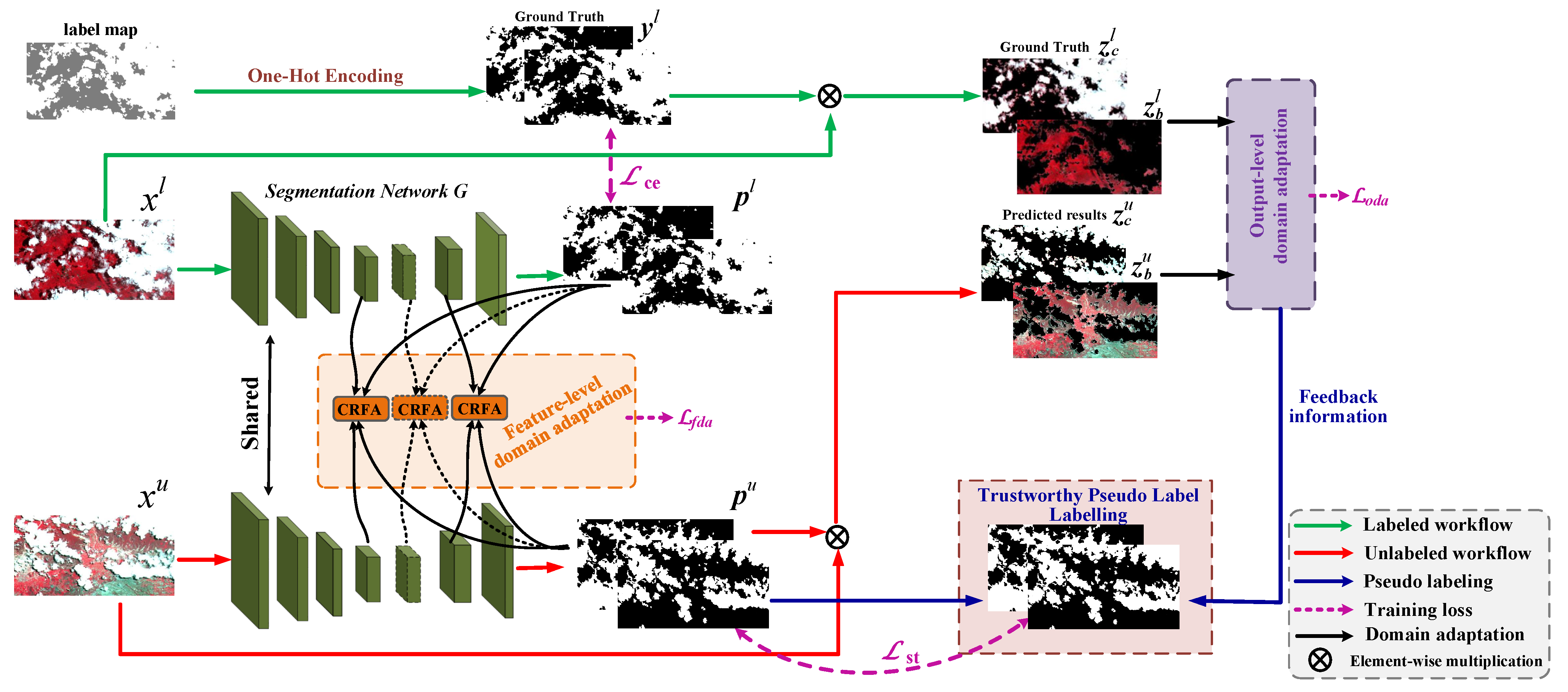
We propose a semi-supervised cloud detection framework, named SSCDnet, which learns knowledge from a limited number of pixel-wise labeled examples and a large number of unlabeled samples for cloud detection.

(ii)

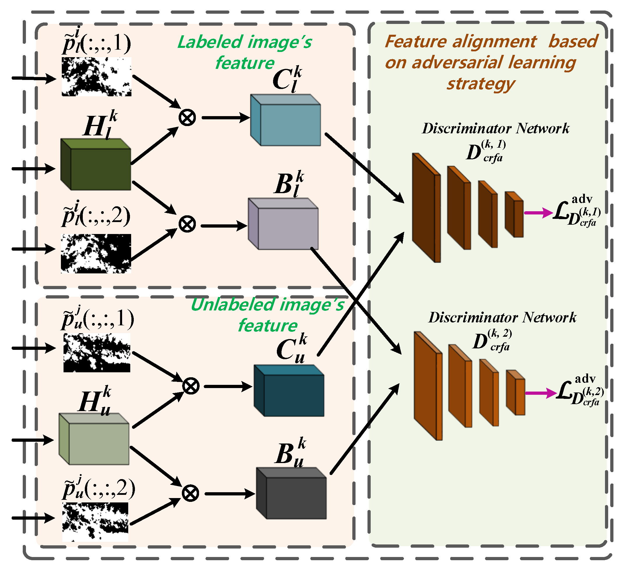
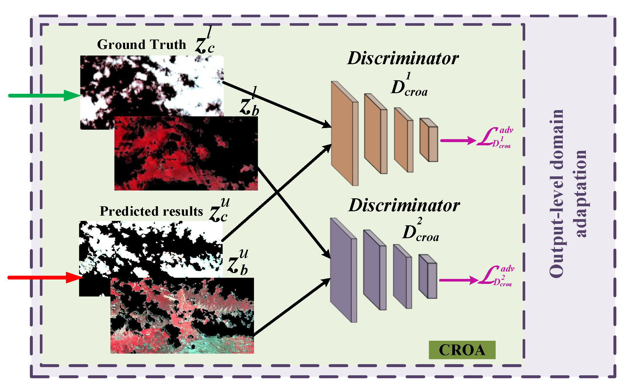
We take the domain shift problem into account between labeled and unlabeled images and propose the feature-level and output-level domain adaptation method to reduce domain distribution gaps.

(iii)

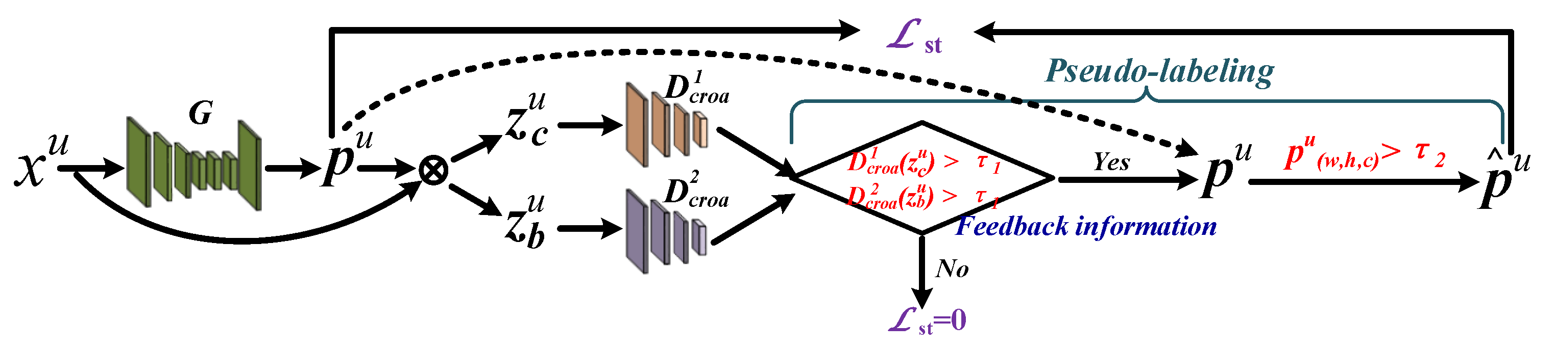
We propose a double threshold pseudo-labeling method to obtain trustworthy pseudo label, which helps to avoid the effects of noise labels for self-training as much as possible and to further enhance the performance of SSCDnet.

This paper is organized as follows: in Section 2, we present the proposed SSCDnet in detail. Experimental datasets and networks training details are presented in Section 4. The experimental results and discussions are presented in Section 4 and Section 5, respectively, followed by conclusions in Section 6.

2. The Proposed Method

In this section, we provide a detailed introduction of the proposed SSCDnet, including the traditional semi-supervised segmentation framework, the proposed overall workflow of SSCDnet, feature/out-level domain adaptation, trustworthy pseudo label labelling, cloud detection network, and discriminator network structures.

2.1. Traditional Semi-Supervised Segmentation Framework

In a traditional semi-supervised segmentation framework [37,38,39,40], as shown in Figure 1, the segmentation network G simultaneously takes advantage of a large number of unlabeled samples and a limited number of labeled examples for a network’s parameter training. In this framework, there are two datasets, i.e., labeled dataset $M^l=\{x^l,y^l\}$ and unlabeled dataset $M^u=\left\{x^u\right\}$, where $x^l$ and $x^u$ are the input data of the segmentation network G and $y^l$ is a pixel-wise label of $x^l$. $p^l$ and $p^u$ represent predicted results of $x^l$ and $x^u$, respectively. ${\widehat{p}}^u$ represents a pseudo label of $p^u$.

During training, given an input labeled image $x^l$, the segmentation network G is supervised by a standard cross-entropy loss ${\mathcal{L}}_{ce}$. When using the unlabeled data $x^u$, the segmentation network is further supervised by a self-training loss ${\mathcal{L}}_{st}$. That is, we use pseudo label ${\widehat{p}}^u$ that generated from predicted result $p^u$ as the “ground truth” for self-training to enhance the semantic segmentation network G. Therefore, total training objective ${\mathcal{L}}_G$ of the segmentation network G is defined as follows:

$${\mathcal{L}}_G={\mathcal{L}}_{ce}+{\lambda }_{st}{\mathcal{L}}_{st},$$

(1)

where ${\lambda }_{st}$ is weight used for minimizing the objective ${\mathcal{L}}_G$.

As shown in Figure 2, remote sensing images obtained from different places show large domain distribution gaps between each other due to different cloud shapes and land-cover types on Earth’s surface. Therefore, there is data drift between labeled samples and unlabeled ones in training dataset of SSL. In SSL framework, segmentation network G trained with labeled samples is hard to generalize to unlabeled ones due to data drift problems. It is difficult to produce a highly certain prediction result $p^u$ for unlabeled sample $x^u$. Predicted results with low certainty leads to low quality pseudo-labels, thus affecting the supervision signal provided from the self-training loss ${\mathcal{L}}_{st}$, and further affecting the performance of segmentation network G. Therefore, improving certainty of predicted results of unlabeled samples is the key to a semi-supervised learning framework.

2.2. Proposed Semi-Supervised Cloud Detection Framework

In this paper, we take the domain shift problem into account for the semi-supervised learning (SSL) framework to improve generalization of the segmentation network to generate trustworthy pseudo-label for self training. We improve a standard SSL network with the unsupervised domain adaptation (UDA) strategy and propose an improved semi-supervised cloud detection network as shown in Figure 3. UDA methods are able to help semantic segmentation networks to learn domain-invariant features at different representation layers, such as input-level (pixel-level) [49], feature-level [45], or output-level [46,47].

Different from the traditional SSL framework, we apply feature-level and output-level domain adaptations at the intermediate layers and the end layer of network, respectively, to reduce domain distribution gaps and improve the generalization performance of SSCDnet. The highly generalized network is able to generate highly certain predicted results for unlabeled samples. To further improve the quality of pseudo-label, instead of directly using the predicted results of unlabeled samples for network training, we proposed a trustworthy pseudo label labelling method to obtain a high-quality pseudo label. To be specific, similar to [40,43], we take advantage of the feedback information from output-level domain adaptation to obtain high-quality candidate labels. Then, we use a threshold strategy to obtain trustworthy regions from the high-quality candidate labels. Finally, trustworthy regions are considered as the ground-truth labels for network training through the self-training loss.

During training, given an input labeled image $x^l$ and its corresponding predicted result is $p^l$, the cloud detection network is supervised by a standard cross-entropy loss ${\mathcal{L}}_{ce}$ [27]. When inputting unlabeled data $x^u$, segmentation network G predicts its corresponding result $p^u$. Then, we generate the pseudo label ${\widehat{p}}^u$ from predicted result $p^u$ by using proposed trustworthy pseudo label labelling method. Pseudo label ${\widehat{p}}^u$ as the “ground truth” for self-training to enhance the semantic segmentation network G. Therefore, the semantic segmentation network is further supervised by self-training loss ${\mathcal{L}}_{st}$ and feature-level domain adaptation loss ${\mathcal{L}}_{fda}$ as well as output-level domain adaptation loss ${\mathcal{L}}_{oda}$ when inputting unlabeled data. The total loss of the semi-supervised cloud detection network, named SSCDnet, is defined as follows:

$${\mathcal{L}}_G={\mathcal{L}}_{ce}+{\lambda }_{st}{\mathcal{L}}_{st}+{\lambda }_{oda}{\mathcal{L}}_{oda}+{\lambda }_{fda}{\mathcal{L}}_{fda},$$

(2)

where ${\lambda }_{st}$, ${\lambda }_{oda}$, and ${\lambda }_{fda}$ are three regulation parameters used for minimizing the objective ${\mathcal{L}}_G$.

During training, we minimize ${\mathcal{L}}_G$ for updating parameters of segmentation network G. The detailed information of the proposed feature/output-level domain adaptation strategies and trustworthy pseudo label labelling method will be introduced in following subsections.

2.3. Reducing Domain Distribution Gaps

2.3.1. Feature-Level Domain Adaptation

To reduce domain distribution gaps at the feature-level, we propose a class-relevant feature alignment (CRFA) strategy. As shown in Figure 4, we use predicted score maps of each class (i.e., cloud and background classes) as the attention maps to obtain class-relevant features. Then, we design a standard binary classification network as the discriminator to help segmentation network $\mathit{G}$ to generate domain-invariant feature representations, thus helping to reduce domain distribution gaps between labeled samples and unlabeled ones at feature level. Therefore, the proposed CRFA domain adaptation consists of two stages: (i) class-relevant feature selection and (ii) class-relevant feature alignment.

To be specific, let ${\mathit{H}}_l^k\in {\mathbb{R}}^{W\times H\times C}$ and ${\mathit{H}}_u^k\in {\mathbb{R}}^{W\times H\times C}$ denote labeled and unlabeled samples’ features extracted from the k-th intermediate hidden layer of network $\mathit{G}$, respectively. Let ${\tilde{p}}_l^i(:,:,1)$ and ${\tilde{p}}_l^i(:,:,2)$ denote the spatial attention maps of cloud and background areas of labeled samples, respectively. Then, cloud-relevant feature ${\mathit{C}}_l^k\in {\mathbb{R}}^{W\times H\times C}$ and background-relevant feature ${\mathit{B}}_l^k\in {\mathbb{R}}^{W\times H\times C}$ of the labeled samples’ feature ${\mathit{H}}_l^k\in {\mathbb{R}}^{W\times H\times C}$ are defined as follows:

$${\mathit{C}}_l^k={\mathit{H}}_l^k\otimes \mathcal{F}\left({\tilde{p}}_l^i(:,:,1)\right),$$

(3)

and

$${\mathit{B}}_l^k={\mathit{H}}_l^k\otimes \mathcal{F}\left({\tilde{p}}_l^i(:,:,2)\right),$$

(4)

where $\mathcal{F}(·)$ represents sampling operator, which includes down-sampling or up-sampling operators. Similarly, we are able to obtain cloud-relevant feature ${\mathit{C}}_u^k\in {\mathbb{R}}^{W\times H\times C}$ and background-relevant feature ${\mathit{B}}_u^k\in {\mathbb{R}}^{W\times H\times C}$ of unlabeled samples’ feature ${\mathit{H}}_u^k\in {\mathbb{R}}^{W\times H\times C}$.

After obtaining these class-relevant features, we input these features into discriminators as shown in Figure 4. For discriminator training, both discriminators ${\mathit{D}}_{\mathrm{crfa}}^{(k,1)}$ and ${\mathit{D}}_{\mathrm{crfa}}^{(k,2)}$ use cross-entropy domain classification loss [44] as the objective function. They are defined as follows:

$$\begin{array}{c}\hfill {\mathcal{L}}_{{\mathit{D}}_{\mathrm{crfa}}^{(k,1)}}=-\mathbb{E}[log\left({\mathit{D}}_{\mathrm{crfa}}^{(k,1)}\left({\mathit{C}}_l^k\right)\right)]-\mathbb{E}[log(1-{\mathit{D}}_{\mathrm{crfa}}^{(k,1)}\left({\mathit{C}}_u^k\right))]\end{array}$$

(5)

and

$$\begin{array}{c}\hfill {\mathcal{L}}_{{\mathit{D}}_{\mathrm{crfa}}^{(k,2)}}=-\mathbb{E}[log\left({\mathit{D}}_{\mathrm{crfa}}^{(k,2)}\left({\mathit{B}}_l^k\right)\right)]-\mathbb{E}[log(1-{\mathit{D}}_{\mathrm{crfa}}^{(k,2)}\left({\mathit{B}}_u^k\right))].\end{array}$$

(6)

For segmentation network training, the adversarial objectives provided by discriminators (${\mathit{D}}_{\mathrm{crfa}}^{(k,1)}$ and ${\mathit{D}}_{\mathrm{crfa}}^{(k,2)}$) are defined as follows:

$${\mathcal{L}}_{{\mathit{D}}_{\mathrm{crfa}}^{(k,1)}}^{adv}=-\mathbb{E}[log{\mathit{D}}_{\mathrm{crfa}}^{(k,1)}\left({\mathit{C}}_u^k\right)]$$

(7)

and

$${\mathcal{L}}_{{\mathit{D}}_{\mathrm{crfa}}^{(k,2)}}^{adv}=-\mathbb{E}[log{\mathit{D}}_{\mathrm{crfa}}^{(k,2)}\left({\mathit{B}}_u^k\right)].$$

(8)

Therefore, the class-relevant feature alignment loss ${\mathcal{L}}_{crfa}^k$ of the k-th intermediate hidden feature is defined as follows:

$${\mathcal{L}}_{crfa}^k={\mathcal{L}}_{{\mathit{D}}_{\mathrm{crfa}}^{(k,1)}}^{adv}+{\mathcal{L}}_{{\mathit{D}}_{\mathrm{crfa}}^{(k,2)}}^{adv}.$$

(9)

Since the proposed feature-level domain adaptation is performed at multiple intermediate layers, the feature-level domain adaptation loss ${\mathcal{L}}_{fda}$ is provided from all intermediate layers’ CRFA losses ${\left\{{\mathcal{L}}_{crfa}^k\right\}}_{k=1}^K$, i.e.,

$${\mathcal{L}}_{fda}=\sum _{k=1}^K{\mathcal{L}}_{crfa}^k.$$

(10)

where ${\mathcal{L}}_{fda}^k$ is the feature domain adaptation loss of the k-th intermediate hidden feature.

2.3.2. Output-Level Domain Adaptation

Instead of directly aligning the predicted results, we align cloud and background objects images extracted from labeled and unlabeled samples, respectively, via a proposed class-relevant outputs alignment (CROA) method. Similar to the CRFA method, the CROA method is built on the standard adversarial learning framework. CROA consists of two discriminators, which are used to align cloud and background images, respectively. As shown in Figure 5, we use two standard binary classification networks as discriminators to reduce the domain distributions gaps between labeled and unlabeled datasets at the output level and improve the certainty of predicted results $z^u$ for unlabeled sample $x^u$.

As shown in Figure 5, we use the cloud and background objects extracted from original images as the input data of different discriminators. To be specific, let $z_c^u=p^u(:,:,1)\otimes x^u$ and $z_b^u=p^u(:,:,2)\otimes x^u$ denote extracted cloud and background objects of unlabeled sample. Similarly, let $z_c^l=p^l(:,:,1)\otimes x^l$ and $z_b^l=p^l(:,:,2)\otimes x^l$ denote extracted cloud and background objects of the labeled sample, where ⊗ represents element-wise multiplication. For discriminator training, both discriminators ${\mathit{D}}_{\mathrm{croa}}^1$ and ${\mathit{D}}_{\mathrm{croa}}^2$ use cross-entropy domain classification loss [44] as the objective function. They are defined as follows:

$$\begin{array}{c}\hfill {\mathcal{L}}_{{\mathit{D}}_{\mathrm{croa}}^1}=-\mathbb{E}[log\left({\mathit{D}}_{\mathrm{croa}}^1\left(z_c^l\right)\right]-\mathbb{E}[log(1-{\mathit{D}}_{\mathrm{croa}}^1\left(z_c^u\right))],\end{array}$$

(11)

and

$$\begin{array}{c}\hfill {\mathcal{L}}_{{\mathit{D}}_{\mathrm{croa}}^2}=-\mathbb{E}[log\left({\mathit{D}}_{\mathrm{croa}}^1\left(z_b^l\right)\right]-\mathbb{E}[log(1-{\mathit{D}}_{\mathrm{croa}}^1\left(z_b^u\right))].\end{array}$$

(12)

For segmentation network training, adversarial objectives provided by these discriminators are defined as follows:

$${\mathcal{L}}_{{\mathit{D}}_{croa}^1}^{adv}=-\mathbb{E}[log{\mathit{D}}_{croa}^1\left(x_c^u\right)],$$

(13)

and

$${\mathcal{L}}_{{\mathit{D}}_{croa}^2}^{adv}=-\mathbb{E}[log{\mathit{D}}_{croa}^2\left(x_b^u\right)].$$

(14)

Therefore, the output-level domain adaptation objective $L_{oda}$ is defined as follows:

$${\mathcal{L}}_{oda}={\mathcal{L}}_{{\mathit{D}}_{croa}^1}^{adv}+{\mathcal{L}}_{{\mathit{D}}_{croa}^2}^{adv}.$$

(15)

As shown in Figure 6, we present the visualized experiment results on a GF-1 WFV image with or without applied domain adaptation. Results show that applying domain adaptation is able to improve the segmentation network to produce high certainly predicted results for unlabeled samples as shown in Figure 6c. High certainly predicted results ensure that we can obtain trustworthy pseudo label for self-training, thus improving the network’s cloud detection performance. More detailed information can be found in Section 4.1 (Ablation Study).

2.4. Trustworthy Pseudo Label Labelling

Pseudo label labelling is the main work for self-training in an SSL framework [38,39,40,43,50]. During self-training, pseudo labels predicted from the segmentation model serve as the “ground truth” to provide additional supervisory signals for network training, which makes the segmentation network able to leverage the unlabeled data. In this paper, we propose a double threshold pseudo-labelling method to efficiently obtain trustworthy regions from pseudo label. We use trustworthy regions as the ground truth for network training.

2.4.1. Candidate Labels Selection

As shown in Figure 7, we sample an unlabeled image $x^u$ into the segmentation network G, obtaining its corresponding predicted probability maps $p^u=\mathit{G}\left(x^u\right)$ as well as extracted cloud and background objects $z_c^u$ and $z_b^u$, respectively. We first use feedback information from the output-level domain adaptation to obtain candidate labels. Specifically, we select high-quality pseudo labels online based on two discriminator scores of output-level domain adaptation, i.e.,

$${\mathit{D}}_{croa}\left(z_c^u\right)>{\tau }_1,{\mathit{D}}_{croa}\left(z_b^u\right)>{\tau }_1,$$

(16)

where ${\tau }_1$ is the threshold. Equation (16) is feedback information from the output-level domain adaptation. We treat these predicted labels satisfied Equation (16) as candidate labels. If not satisfied, we directly set self-training loss ${\mathcal{L}}_{st}=0$.

2.4.2. Trustworthy Regions Selection from Candidate Labels

After we obtained the candidate labels, we set a confidence threshold ${\tau }_2$ to discover trustworthy regions from the selected candidate labels, i.e.,

$${\mathit{D}}_{croa}^1\left(z_c^u\right)>{\tau }_1,{\mathit{D}}_{croa}^2\left(z_b^u\right)>{\tau }_1,and{p}_{(w,h,c)}^u>{\tau }_2.$$

(17)

Equation (17) indicates that, if predicted probability of these regions is greater than ${\tau }_2$, we use these trustworthy regions as the ground-truth for self-training.

2.4.3. Self-Training Loss ${\mathcal{L}}_{st}$

According to the above mentioned method, the self-training loss ${\mathcal{L}}_{st}$ is defined as:

$${\mathcal{L}}_{st}=\left\{\begin{array}{cc}-\sum {\widehat{p}}_{(w,h,c)}^{u}log{p}_{(w,h,c)}^u,& {\mathit{D}}_{croa}^1\left(z_c^u\right)>{\tau }_1,{\mathit{D}}_{croa}^2\left(z_b^u\right)>{\tau }_1,\\ & and{p}_{(w,h,c)}^u>{\tau }_2\\ & \\ 0& \mathrm{otherwise}.\end{array}\right.$$

(18)

where ${\widehat{p}}^u$ is the pseudo label generated from the prediction map $p^u$ by using a one-hot encoding scheme. $p_{(w,h,c)}^u$ represents the predicted probability at the location (h,w) of the C-channel.

2.5. Network Architecture

2.5.1. Cloud Detection Network

Similar to most SSL approaches [40,43], we use DeepLabv2 [51] as our main cloud detection framework and resort to ResNet-101 [52] as the backbone to extract semantic segmentation information. DeepLabv2 uses atrous spatial pyramid pooling (ASPP) module [51], which incorporates multiple parallel dilated convolutional layers [53] with different sampling rates, to capture multi-scale features for robustness clouds detection. In this paper, we set the resolution of predicted probability map as 1/8 × 1/8 size of input image for fair comparison with previous semi-supervised works based on DeepLabv2, such as [37,40]. Then, we directly up-sample the predicted probability maps to the same size as the input images to obtain final predicted results.

2.5.2. Discriminator Network

In this paper, we design a standard binary classification network as the discriminator for both CRFA and CROA modules. Figure 8 illustrates the detailed structure of the designed discriminator. This discriminator contains four convolutional layers, a global average pooling layer, and a fully-connected layer. To be specific, there are four convolutional layers with 4 × 4 kernels. Four convolutional layers have $\{256,192,128,64\}$ and $\{64,128,256,512\}$ channels for CRFA and CROA modules, respectively. Each convolutional layer shares the same stride (stride = 2) and simultaneously followed by a Leaky-ReLU activation (slope = 0.2) and a dropout layer (dropout-rate = 0.5). After these convolution operations, a global average pooling layer and a fully-connected layer are designed to obtain confidence score for each input image.

3. Dataset and Experimental Settings

3.1. Experimental Dataset

In this paper, we use two available cloud cover validation datasets, i.e., Landsat-8 OLI cloud cover validation dataset [48] and GF-1 WFV cloud and cloud shadow cover validation dataset [12], to comprehensively evaluate the proposed SSCDnet.

Table 1. The detailed information of Landsat-8 OLI and GF1-WFV multispectral images.

Sensor	Spectral Band	Wavelength Range ($\mathsf{\mu }$m)	Spatial Resolution (m)
Landsat-8 OLI	Band 1 (coastal)	0.433–0.453	30
	Band 2 (blue)	0.450–0.515	30
	Band 3 (green)	0.525–0.600	30
	Band 4 (red)	0.630–0.680	30
	Band 5 (NIR)	0.845–0.885	30
	Band 6 (SWIR1)	1.560–1.660	30
	Band 7 (SWIR2)	2.100–2.300	30
	Band 8 (Pan)	0.500–0.680	15
	Band 9 (Cirrus)	1.360–1.390	30
GF-1 WFV	Band 1 (blue)	0.450–0.520	16
	Band 2 (green)	0.520–0.590	16
	Band 3 (red)	0.630–0.690	16
	Band 4 (NIR)	0.770–0.890	16

shows the detailed information of Landsat-8 OLI and GF1-WFV multispectral images. Similar to [27], we follow the idea that the number of subimages with and without cloud in the training data should be balanced. Otherwise, the detection results would bias towards the majority. Therefore, we exclude some cloud-free and full cloud covered scenes. In addition, current cloud detection accuracy measurement is not robust when the cloud percentage is quite low [10]. A low cloud cover percentage in a scene may cause an apparent reduction in the cloud’s producer accuracy and user accuracy. Therefore, original large size images with cloud percentage less than 5% are usually removed in training and testing. Finally, we select 40 and 20 scenes images from both Landsat-8 and Gaofen-1 WFV dataset for network training and evaluation, respectively.

As illustrated in [54], CNNs are strongly biased towards recognizing textures for object classification. Therefore, we can select a limited number of channels data of multispectral data to evaluate the proposed SSCDnet. In this paper, we select channels 3 (green), 4 (red), and 5 (near-infrared) of Landsat-8 OLI data and channels 2 (green), 3 (red), and 4 (near-infrared) of Gaofen-1 WFV data for segmentation network training and testing. During training, all training data are cropped into subimages of pixel size 321 × 321. There are about 30 k and 75 k annotated sub-images in Landsat-8 OLI and GF-1 WFV training dataset, respectively. We select a portion of the data set for network supervised training and the remaining de-annotated portion for network self-training (unsupervised training). During testing, we divide the whole RS image into a series of sub-images with image size of 1200 × 1200 for network evaluation. The final detection result is obtained by merging results of sub-images.

3.2. Network Training Details and Parameters Setting

SSCDnet is trained under PyTorch framework (https://pytorch.org/, accessed on 24 April 2022). The operating system is Ubuntu 14.04 equipped with NVIDIA GTX 1080 Ti GPU. We optimize the segmentation (generator) and discriminator networks by using SGD algorithm [55] and Adam optimizer [56], respectively. During training, these two datasets share the following parameters settings. That is, learning rates for generator and discriminator network are 2.5 ×${10}^{-4}$ and 1 ×${10}^{-4}$, respectively. Training decay policy is “poly” [57]. The number of mini-batch size, momentum, and weight decay are 4, 0.9, and 5 × ${10}^{-4}$, respectively. SSCDnet is trained for 20 and 15 epochs on Landsat-8 OLI and GF-1 WFV dataset, respectively.

In addition, in order to improve the performance, we use the model pre-trained on the ImageNet dataset [58] to fine-tune the parameters of the backbone network (ResNet-101). We conduct feature-level domain adaptation tasks at the end of $Conv4\_x$ and $Conv5\_x$ residual blocks, i.e., $K=2$. We empirically set weight-parameters ${\lambda }_{st}=1.0$, ${\lambda }_{fda}=0.001$, and ${\lambda }_{oda}=0.1$ for GF-1 dataset, set ${\lambda }_{st}=1.0$, ${\lambda }_{fda}=0.001$, and ${\lambda }_{oda}=0.01$ for Landsat-8 OLI dataset. In addition, we empirically set threshold-parameters ${\tau }_1=0.6$ and ${\tau }_2=0.55$ to accurately generate trustworthy pseudo labels for both GF-1 and Landsat-8 OLI datasets.

4. Experimental Results

4.1. Ablation Study

To investigate the effectiveness of SSCDnet, we conduct a series of ablation studies on it. Five widely used quantitative metrics of RS images, i.e., mean intersection over union (MIoU), kappa coefficient (Kappa), overall accuracy (OA), producer accuracy (PA), and user accuracy (UA), are used to comprehensively measure the cloud detection results. All experiment results are obtained from the GF-1 WFV dataset.

4.1.1. Ablation Study on Loss Function

In this paper, the proposed SSCDnet is supervised by four loss functions, i.e., a standard cross-entropy loss $L_{ce}$, self-training loss $L_{st}$, output-level domain adaptation loss $L_{oda}$, and feature-level domain adaptation loss $L_{fda}$. In

Table 2. Cloud extraction accuracy (%) of different ablation networks on GF-1 WFV data.

Proportions	${\mathcal{L}}_{\mathit{c}\mathit{e}}$	√	√	√	√
	${\mathcal{L}}_{st}$	×	√	√	√
	${\mathcal{L}}_{oda}$	×	×	√	√
	${\mathcal{L}}_{fda}$	×	×	×	√
$\frac{1}{200}$	OA	90.22	93.56	95.30	95.51
	MIoU	71.77	83.22	86.95	87.54
	Kappa	68.21	78.15	82.07	82.69
	PA	67.03	73.67	80.02	81.28
	UA	95.51	96.40	94.57	93.55
$\frac{1}{100}$	OA	91.34	93.89	95.73	95.85
	MIoU	74.10	84.11	88.05	88.90
	Kappa	71.51	78.90	83.34	83.92
	PA	69.71	74.32	81.52	82.34
	UA	94.93	95.99	94.28	93.36
$\frac{1}{40}$	OA	92.23	94.52	96.02	96.24
	MIoU	76.02	86.03	89.01	89.30
	Kappa	73.58	80.85	84.77	85.01
	PA	75.08	80.18	84.40	85.49
	UA	93.43	93.30	91.59	92.24
$\frac{1}{20}$	OA	93.19	95.11	96.55	96.90
	MIoU	79.88	87.16	90.46	90.93
	Kappa	75.75	83.77	86.25	86.97
	PA	80.69	82.22	84.87	85.89
	UA	92.30	92.10	92.72	92.24
Full	OA	96.91	97.11	97.17	97.19
	MIoU	90.15	91.50	91.67	91.71
	Kappa	88.64	89.49	89.35	89.37
	PA	87.28	88.67	88.84	88.90
	UA	92.05	92.33	92.51	92.32

where $\frac{1}{200}$, $\frac{1}{100}$, $\frac{1}{40}$, and $\frac{1}{20}$ are the fractions of the total training images in the dataset that are used as labeled data, and the rest of the data was used without labels. Bold indicates maximum value in this paper.

, we list ablation results under different proportion of labeled samples ($\frac{1}{200}$, $\frac{1}{100}$, $\frac{1}{40}$, $\frac{1}{20}$, and full labeled samples) to demonstrate the effects of each component loss.

Results in Table 2 show that the best performance is achieved by a combination of all optimal loss terms (we use $\{{\mathcal{L}}_{ce},{\mathcal{L}}_{st},{\mathcal{L}}_{oda},{\mathcal{L}}_{fda}\}$ to represent this combination.), while the baseline framework supervised only by the standard cross-entropy loss ${\mathcal{L}}_{ce}$ shows the worst performance. To be specific, a combination of ${\mathcal{L}}_{ce}$ and ${\mathcal{L}}_{st}$ (i.e., $\{{\mathcal{L}}_{ce},{\mathcal{L}}_{st}\}$) and combination of ${\mathcal{L}}_{ce}$, ${\mathcal{L}}_{st}$, and ${\mathcal{L}}_{oda}$ (i.e., $\{{\mathcal{L}}_{ce},{\mathcal{L}}_{st},{\mathcal{L}}_{oda}\}$) obtain significant improvement of +9.44% and +13.86% in Kappa, respectively, compared with only ${\mathcal{L}}_{ce}$ loss when labeled sample proportion is $\frac{1}{200}$. In addition, $\{{\mathcal{L}}_{ce},{\mathcal{L}}_{st}\}$ and $\{{\mathcal{L}}_{ce},{\mathcal{L}}_{st},{\mathcal{L}}_{oda}\}$ also outperform ${\mathcal{L}}_{ce}$ under other proportions of labeled sample settings, which shows that output-level domain adaptation and self-training strategies are able to improve the performance of segmentation network.

Based on $\{{\mathcal{L}}_{ce},{\mathcal{L}}_{st},{\mathcal{L}}_{oda}\}$, we further introduce feature domain adaptation loss ${\mathcal{L}}_{fda}$ to reduce feature-level domain distribution gaps between labeled and unlabeled datasets. Results in Table 2 show that $\{{\mathcal{L}}_{ce},{\mathcal{L}}_{st},{\mathcal{L}}_{oda},{\mathcal{L}}_{fda}\}$ performs better than $\{{\mathcal{L}}_{ce},{\mathcal{L}}_{st},{\mathcal{L}}_{oda}\}$. In addition, it can be seen that the performance of $\{{\mathcal{L}}_{ce},{\mathcal{L}}_{st},{\mathcal{L}}_{oda},{\mathcal{L}}_{fda}\}$ consistently outperforms those of other combinations under different proportions of labeled sample ($\{\frac{1}{200},\frac{1}{100},\frac{1}{40},\frac{1}{20}\}$), which shows that the proposed $\{{\mathcal{L}}_{ce},{\mathcal{L}}_{st},{\mathcal{L}}_{oda},{\mathcal{L}}_{fda}\}$ is a promising strategy for semi-supervised segmentation network.

In summary, results in Table 2 demonstrate that standard cross-entropy loss ${\mathcal{L}}_{ce}$, self-training loss ${\mathcal{L}}_{st}$, output-level domain adaptation loss ${\mathcal{L}}_{oda}$, and feature-level domain adaptation loss ${\mathcal{L}}_{fda}$ are beneficial for semi-supervised cloud detection work. Because applying domain adaptation strategy is able to reduce distribution gaps between labeled and unlabeled datasets and improve SSCDnet to generate trustworthy pseudo-labels for self-training, thus providing positive supervised signals for segmentation network learning. Combination of all these loss terms is able to achieve a state-of-the-art cloud detection performance when using a limited number of labeled samples.

4.1.2. Ablation Study on Feature-Level Domain Adaptation

In this paper, we use ResNet-101 [52] as the backbone network to extract feature maps and conduct domain adaptation study on the end features of $Conv4\_x$, $Conv5\_x$, $Conv3\_x$, and $Conv2\_x$ residual blocks. In

Table 3. Ablation study of domain adaptation on different intermediate layers (proportion = $\frac{1}{200}$).

Methods	OA	MIoU	Kappa	PA	UA
FDA_5	95.40	87.11	82.53	80.28	94.68
FDA_45	95.51	87.54	82.69	81.28	93.55
FDA_345	95.13	86.17	81.64	79.19	94.89
FDA_2345	95.41	87.06	82.93	81.73	93.54

, we list the experiment results of ablation study on different intermediate layers. Experiment results show that applying feature domain adaptation on the end of $Conv4\_x$ and $Conv5\_x$ residual blocks, i.e., FDA_45, achieves the best performance. In contrast, applying feature domain adaptation on other layers’ features always shows worse performance than on $Conv4\_x$ and $Conv5\_x$ layers. Hence, we conduct the domain adaptation tasks at the end of $Conv4\_x$ and $Conv5\_x$ residual blocks (two intermediate layers $K=2$ in feature-level domain adaptation). Furthermore, we find that applying domain adaptation tasks at above mentioned intermediate layers is able to achieve promising performance on the Landsat-8 OLI dataset.

4.1.3. Ablation Study on Self-Training’s Double Threshold

In this paper, we proposed a double threshold method to obtain trustworthy pseudo labels for network self-training. In

Table 4. Ablation study on double threshold (proportion = $\frac{1}{200}$).

Methods	OA	MIoU	Kappa	PA	UA
${\mathcal{L}}_{st}{}_{(N/A,N/A)}$	94.12	85.02	81.43	79.38	94.74
${\mathcal{L}}_{st}{}_{({\tau }_1,N/A)}$	95.02	86.33	81.95	80.11	93.30
${\mathcal{L}}_{st}{}_{({\tau }_1,{\tau }_2)}$	95.30	86.95	82.07	80.02	94.57

, we investigate effectiveness of the proposed pseudo-labeling method.

In Table 4, we list the experiment results under different pseudo-labeling strategies, i.e., pseudo-labeling directly transforms from probability maps ${\mathcal{L}}_{st}{}_{(N/A,N/A)}$, pseudo-labeling based on a discriminator score of output-level domain adaptation ${\mathcal{L}}_{st}{}_{({\tau }_1,N/A)}$, and pseudo-labeling based on both discriminator score of output-level domain adaptation and trustworthy regions selection ${\mathcal{L}}_{st}{}_{({\tau }_1,{\tau }_2)}$, where ${\tau }_1$ and ${\tau }_2$ are used to obtain candidate labels and trustworthy regions, respectively. Results in Table 4 show that performance of the loss term ${\mathcal{L}}_{st}{}_{({\tau }_1,{\tau }_2)}$ is better than those of ${\mathcal{L}}_{st}{}_{({\tau }_1,N/A)}$ and ${\mathcal{L}}_{st}{}_{(N/A,N/A)}$, which demonstrates that trustworthy regions selection based on high confidence candidate label is a promising strategy for pseudo label selecting.

4.1.4. Hyper-Parameter Analysis

The proposed training objective ${\mathcal{L}}_G$ has three balance weights, i.e., ${\lambda }_{st}$, ${\lambda }_{oda}$, and ${\lambda }_{fda}$. In this paper, since we use all the trustworthy regions’ pseudo labels for self-training, we directly set ${\lambda }_{st}=1.0$. Then, ${\lambda }_{oda}$ and ${\lambda }_{fda}$ are two important hyper-parameters that affect cloud detection results. In

Table 5. The study on hyper-parameter ${\lambda }_{st}$, ${\lambda }_{oda}$, and ${\lambda }_{fda}$ (proportion = $\frac{1}{200}$).

${\mathit{\lambda }}_{\mathit{st}}$	${\mathit{\lambda }}_{\mathit{oda}}$	${\mathit{\lambda }}_{\mathit{fda}}$	OA	MIoU	Kappa	PA	UA
1.0	0.05	N/A	93.05	83.66	80.80	77.90	94.51
1.0	0.10	N/A	93.48	84.74	81.51	79.02	93.61
1.0	0.15	N/A	93.12	84.10	81.18	78.60	94.19
1.0	0.10	0.10	92.26	81.12	72.61	68.53	94.79
1.0	0.10	0.01	94.96	85.86	81.43	80.06	93.48
1.0	0.10	0.001	95.51	87.54	82.69	81.28	93.55
1.0	0.10	0.005	95.40	87.11	82.68	80.35	94.86

, we list a series of validation experimental results to investigate the impact of these hyper-parameters. As illustrated in Table 5, we first obtain the promising ${\lambda }_{oda}$ by setting ${\lambda }_{fda}=N/A$ (N/A means Not Applicable). Then, we obtain the promising ${\lambda }_{fda}$ based on obtained promising ${\lambda }_{oda}$. Experimental results in Table 5 show that setting ${\lambda }_{oda}=0.10$ and ${\lambda }_{fda}=0.001$ is able to achieve promising performance. Similarly, we can obtain the promising hyper-parameter setting based on above mentioned methods on Landsat-8 OLI data cloud detection task.

4.2. Comparisons with State-of-the-Art Methods

4.2.1. Comparison Methods

For comprehensive evaluation, we compare deep adversarial network DAN [37], which focuses on training with both un-labeled and labeled images simultaneously to improve segmentation performance. Moreover, we compare two semi-supervised CNN-based semantic segmentation methods, i.e., Hung et al. [43] and s4GAN [40]. These two SSL methods are based on an adversarial network and achieve promising performance on PASCAL VOC 2012 [59] and Cityscapes datasets [36]. For fair comparison with the proposed SSCDnet, we use DeepLabv2 [51] and ResNet-101 [52] as a segmentation network and backbone of above-mentioned competing methods, respectively. In addition, baseline network DeepLabv2 [51] is also used as the competing method. During training, we retrain these CNN-based methods under their optimal parameter settings on Landast-8 OLI and GF-1 WFV datasets.

4.2.2. Results on GF-1 WFV Data

Table 6. Cloud extraction accuracy (%) of different comparison networks on GF-1 WFV data. All results are the averaging results on all testing images.

Proportion	Methods	OA	MIoU	Kappa	PA	UA
$\frac{1}{200}$	DeepLabV2 [51]	90.22	71.77	68.21	67.03	95.51
	DAN [37]	92.59	79.93	74.65	72.08	94.59
	Hung et al. [43]	93.01	81.20	75.11	76.59	94.02
	s4GAN [40]	93.44	81.79	75.62	77.31	93.38
	SSCDnet	95.51	87.54	82.69	81.28	93.55
$\frac{1}{100}$	DeepLabV2 [51]	91.34	74.10	71.51	69.71	94.93
	DAN [37]	93.13	82.41	77.56	75.84	93.66
	Hung et al. [43]	94.20	83.88	78.56	76.11	93.02
	s4GAN [40]	94.60	84.91	79.14	76.47	92.63
	SSCDnet	95.85	88.90	83.92	82.34	93.36
$\frac{1}{40}$	DeepLabV2 [51]	92.23	76.02	73.58	75.08	93.43
	DAN [37]	93.89	83.63	80.15	81.29	92.53
	Hung et al. [43]	94.41	85.05	81.59	81.80	92.76
	s4GAN [40]	95.30	86.80	82.47	82.20	93.00
	SSCDnet	96.24	89.30	85.01	85.49	92.24
$\frac{1}{20}$	DeepLabV2 [51]	93.19	79.88	75.75	80.69	92.30
	DAN [37]	94.32	85.05	81.52	82.21	92.93
	Hung et al. [43]	94.94	86.12	82.53	82.44	93.09
	s4GAN [40]	95.61	87.18	83.63	82.96	93.37
	SSCDnet	96.90	90.93	86.97	85.89	92.24
Full	DeepLabV2 [51]	96.11	90.15	87.64	87.28	92.15
	DAN [37]	97.09	90.37	88.72	88.19	92.43
	Hung et al. [43]	97.12	90.57	88.79	88.50	92.71
	s4GAN [40]	97.16	90.88	88.83	88.57	92.60
	SSCDnet	97.19	91.71	89.37	88.90	92.32

where $\frac{1}{200}$, $\frac{1}{100}$, $\frac{1}{40}$, and $\frac{1}{20}$ are the fractions of the total training images in the dataset that are used as labeled data, and the rest of the data are used without labels.

shows the quantitative results in terms of average OA, MIoU, Kappa, PA, and UA on the GF-1 WFV testing dataset. We show these comparison results on four different proportions of labeled samples ($\frac{1}{200}$, $\frac{1}{100}$, $\frac{1}{40}$, and $\frac{1}{20}$). Meanwhile, we also give comparison results on fully labeled samples. Experiment results show that our proposed SSCDnet consistently outperforms these competing methods at different proportions of labeled samples. Notably, SSCDnet achieves 83.08% Kappa and 86.96% MIoU using only 0.5% (1/200) training data with pixel-wise annotation. Results of SSCDnet significantly outperform those of competing methods. SSCDnet also achieves the best performance on fully labeled data and shows a larger gain in terms of OA, MIoU, Kappa, PA, and UA than competing methods.

It can be seen that the baseline network, DeepLabV2 [51], trained with only labeled data, shows the worst results. DAN [37] shows better results than DeepLabV2 [51] due to it being able to effectively utilize unlabeled data for training. These semi-supervised methods, Hung et al. [43] and s4GAN [40] show better results than DeepLabV2 [51] and DAN [37] due to being able to learn knowledge from a limited number of labeled examples and a large number of additional unlabeled samples. Although these two methods show competitive cloud detection performance, there is still a gap in performance between them and the proposed SSCDnet. In addition, it also can be seen that all of the methods show promising cloud detection performance on GF-1 WFV data when using fully labeled data for network training. Even the worst baseline method DeepLabV2 [51] achieves 90.15% mIoU and 88.64% Kappa.

In Figure 9, we show qualitative results when labeled samples proportion is $\frac{1}{200}$. These images contain typical land-cover types, i.e., Figure 9a includes mountains, wetlands, farmland, and grass/crops, Figure 9b includes village, forest and ice/snow, Figure 9c includes water. Experiment results show that detection results of SSCDnet show more consistency with the ground-truth than those of other competing methods. Results of competing methods show a lot of misclassification pixels in thin cloud areas, while SSCDnet shows less misclassification pixels, which indicates that SSCDnet is able to achieve more promising performance on these imageries when using a limited number of labeled images.

4.2.3. Results on Landsat-8 OLI Data

In addition to the experiment results on the GF-1 data, we also conduct experiments on Landsat8 OLI data. In Table 7, we list quantitative results on the Landsat8 OLI testing dataset. Compared to other methods, the proposed SSCDnet also performs best on Landsat8 OLI data. For the low labeled sample’s proportion, such as $\frac{1}{200}$, SSCDnet is still able to achieve satisfactory results (90.77% MIoU and 88.72% Kappa). These results show consistency with the ground-truth. In contrast, performance of these competing methods is less than that of SSCDnet. When increasing the proportion of labeled samples, competing methods can improve their performance, but they are still inferior to SSCDnet. From Table 7, we find that the performance of SSCDnet at a labeled sample proportion of $\frac{1}{20}$ approaches that of its full supervision and outperforms fully supervised DeepLabV2 [51] and DAN [37]. For fully labeled data, with the help of adversarial training and self-training strategies, SSCDnet still shows the best performance compared with other competing methods.

In Figure 10, we show qualitative results on three whole scene landsat-8 OLI images. These images contain typical land-cover types, i.e., Figure 10a includes mountains, forest, ice/snow, water, and wetlands areas. Figure 10b includes water, floating ice, urban, mountains, and forest areas. Figure 10c includes barren and desert areas. Experiment results are obtained when labeled sample proportion is $\frac{1}{200}$. Experiment results show that SSCDnet trained with a limited number of labeled samples can yield very competitive performance on Landsat-8 OLI data. It can be seen that results of these competing methods show a large number of misclassified pixels (red areas), especially in Figure 10c. There are a large number of misclassified pixels displayed in the thin cloud area. In contrast, SSCDnet works well on these images. Results of SSCDnet shows better consistency with the ground-truth and fewer misclassified pixels than competing methods. Overall, experiment results in Table 7 and Figure 10 show that the proposed SSCDnet is able to achieve promising cloud detection performance on Landsat-8 OLI data.

Table 7. Cloud extraction accuracy (%) of different comparison networks on Landsat-8 OLI data. All results are the averaged results on all the testing images.

Proportions	Method	OA	MIoU	Kappa	PA	UA
$\frac{1}{200}$	DeepLabV2 [51]	91.24	84.16	81.77	82.12	94.53
	DAN [37]	92.68	86.97	82.83	90.47	88.78
	Hung et al. [43]	93.14	87.02	84.49	91.55	90.13
	s4GAN [40]	93.88	88.76	85.91	93.38	91.05
	SSCDnet	95.48	91.28	88.87	95.60	90.62
$\frac{1}{100}$	DeepLabV2 [51]	92.54	88.76	85.06	88.30	89.41
	DAN [37]	93.99	89.32	85.75	91.11	89.45
	Hung et al. [43]	94.58	90.71	87.89	93.80	90.33
	s4GAN [40]	95.40	91.30	89.02	94.17	91.08
	SSCDnet	95.63	91.75	89.38	93.81	92.01
$\frac{1}{40}$	DeepLabV2 [51]	93.15	89.06	85.67	90.16	89.90
	DAN [37]	94.37	89.26	86.78	92.38	89.77
	Hung et al. [43]	94.79	90.93	88.11	93.22	91.05
	s4GAN [40]	95.54	91.33	89.19	93.15	92.00
	SSCDnet	95.82	92.03	89.61	93.18	92.31
$\frac{1}{20}$	DeepLabV2 [51]	94.12	89.33	86.45	91.85	90.36
	DAN [37]	95.29	89.61	86.99	92.67	90.14
	Hung et al. [43]	95.83	91.06	88.20	92.11	91.82
	s4GAN [40]	96.16	91.96	89.69	92.04	92.84
	SSCDnet	96.67	92.19	90.13	92.50	93.26
Full	DeepLabV2 [51]	96.56	91.03	89.25	91.10	91.26
	DAN [37]	96.60	92.09	89.53	91.62	93.11
	Hung et al. [43]	96.57	92.11	89.77	92.28	92.03
	s4GAN [40]	96.63	92.06	89.82	92.16	92.41
	SSCDnet	97.19	92.65	90.34	92.75	93.36

Table 7. Cloud extraction accuracy (%) of different comparison networks on Landsat-8 OLI data. All results are the averaged results on all the testing images.

Proportions	Method	OA	MIoU	Kappa	PA	UA
$\frac{1}{200}$	DeepLabV2 [51]	91.24	84.16	81.77	82.12	94.53
	DAN [37]	92.68	86.97	82.83	90.47	88.78
	Hung et al. [43]	93.14	87.02	84.49	91.55	90.13
	s4GAN [40]	93.88	88.76	85.91	93.38	91.05
	SSCDnet	95.48	91.28	88.87	95.60	90.62
$\frac{1}{100}$	DeepLabV2 [51]	92.54	88.76	85.06	88.30	89.41
	DAN [37]	93.99	89.32	85.75	91.11	89.45
	Hung et al. [43]	94.58	90.71	87.89	93.80	90.33
	s4GAN [40]	95.40	91.30	89.02	94.17	91.08
	SSCDnet	95.63	91.75	89.38	93.81	92.01
$\frac{1}{40}$	DeepLabV2 [51]	93.15	89.06	85.67	90.16	89.90
	DAN [37]	94.37	89.26	86.78	92.38	89.77
	Hung et al. [43]	94.79	90.93	88.11	93.22	91.05
	s4GAN [40]	95.54	91.33	89.19	93.15	92.00
	SSCDnet	95.82	92.03	89.61	93.18	92.31
$\frac{1}{20}$	DeepLabV2 [51]	94.12	89.33	86.45	91.85	90.36
	DAN [37]	95.29	89.61	86.99	92.67	90.14
	Hung et al. [43]	95.83	91.06	88.20	92.11	91.82
	s4GAN [40]	96.16	91.96	89.69	92.04	92.84
	SSCDnet	96.67	92.19	90.13	92.50	93.26
Full	DeepLabV2 [51]	96.56	91.03	89.25	91.10	91.26
	DAN [37]	96.60	92.09	89.53	91.62	93.11
	Hung et al. [43]	96.57	92.11	89.77	92.28	92.03
	s4GAN [40]	96.63	92.06	89.82	92.16	92.41
	SSCDnet	97.19	92.65	90.34	92.75	93.36

5. Discussion and Analysis

5.1. Robustness Analysis

To evaluate the robustness of the proposed method, we conducted a series of experiments as follows: (1) experiment results on the same area under different seasons and (2) experiment results on different land cover types.

5.1.1. Results on the Same Area under Different Seasons

In Figure 11, we present the cloud detection results on the same area under different seasons, i.e., Spring, Summer, Autumn, and Winter. Satellite images obtained from this area include different land cover types, such as mountain, village, urban, water, ocean, plant, and farmland areas. In Figure 11, overall accuracy (OA) of Spring, Summer, Autumn, and Winter images are 98.21%, 97.70%, 95.79%, and 96.03%, respectively. Experiment results show that the proposed semi-supervised cloud detection method SSCDnet is able to achieve a promising performance under different radiance (i.e., same area and different seasons). However, there is still a large number of misclassified pixels in the experiment results. These misclassified pixels are located mostly near the cloud object boundaries and thin cloud areas, which is also a difficult problem for most CNN-based cloud detection works, such as [7,19,27,33,34,35].

5.1.2. Results on Different Land Cover Types

In Figure 12, we present the experiment results on twelve sub images with different land cover types. Results show that these corresponding cloud detection results obtained by SSCDnet show consistency with the ground truth when our CNN model is trained with a limited number of labeled dataset (labeled proportion is $\frac{1}{10}$), except for some misclassified pixels located near cloud object boundaries and thin cloud areas.

To be specific, for tough cases, such as barren/desert areas (Figure 12a,b) and urban areas (Figure 12g,h), SSCDnet is able to achieve a promising performance on these land cover types. In addition, SSCDnet also shows promising performance on water areas, such as lake (Figure 12i,j), river (Figure 12h), and ocean (Figure 12k,l) areas. Except for snow, buildings, and some white objects, few ground objects affect cloud detection, and SSCDnet can easily obtain promising results in some general cases, such as mountain/plant (Figure 12e,f) and farmland/village (Figure 12g,h) areas. In general, results in Figure 12 demonstrate that SSCDnet has a robust cloud detection performance on different land cover types.

5.2. Computational Complexity Analysis

To analyze the computational complexity of SSCDnet, we evaluate computational complexity of these networks with six evaluation criterions, which are floating point operations (FLOPs), number of trainable parameters, training time, training GPU memory usage, testing time, and testing GPU memory usage. In Table 8, we list results of different competing methods. FLOPs are calculated from input data with image size of 321 × 321. Training times of all methods are obtained from 5000 iterations. Training GPU memory size is obtained by setting batch size of 4 and image size of 321 × 321. Testing time is obtained by testing 20 scene Landsat-8 OLI satellite images with image size of 8 k × 8 k. Training GPU memory size is obtained by setting batch size of 1 and image size of 1200 × 1200.

During training, both the segmentation network and discriminator network are trained simultaneously. Discriminators of different SSL methods have different raw input data channels, which results in these models having different model parameters, different computational complexity and training times, and different GPU memory requirements. In Table 8, we can see that FLOPs, number of parameters, and training GUP memory usage of SSCDnet are higher than those of competing methods. This is because SSCDnet performs intermediate feature map domain adaptation alignments, while competing methods have no such operation. Feature map alignment requires more computations and GPU memories. In addition, the discriminator network for feature alignment further increases the number of training parameters. Luckily, the longest training time is not the SSCDnet but Hung et al. [43].

During testing, we only need to use the segmentation network to detect clouds instead of the discriminator network. Since all the methods use the same baseline segmentation network, i.e., DeepLabV2 [51], all these methods share the same testing times and GPU memory usage. In Table 8, we can see that it takes about 400 s to detect 20 scenes Landsat 8-OLI satellite images with image size of 8 k × 8 k. In other words, it takes 20 s to detect an image. 2849 MB GPU memory is required to process an image with size of 1200 × 1200.

Table 8. Computational complexity analysis of different semi-supervised methods and the baseline method (DeepLabV2 [51]).

Methods	GFLOPs	Parameters	Training Time	Training GPU	Testing Time	Testing GPU
DeepLabV2 [51]	74.03	43.94 M	1118.9906 s	10,079 MB	400.7494 s	2849 MB
DAN [37]	76.67	46.70 M	2129.5402 s	10,297 MB	400.7494 s	2849 MB
Hung et al. [43]	76.61	46.70 M	10,178.0476 s	10,297 MB	400.7494 s	2849 MB
s4GAN [40]	76.68	46.70 M	2224.8972 s	10,341 MB	400.7494 s	2849 MB
SSCDnet	410.56	61.91 M	2771.0219 s	10,435 MB	400.7494 s	2849 MB

The code for computational complexity is available from https://github.com/sovrasov/flops-counter.pytorch (accessed on 24 April 2022). 1 GFLOPs = 1 × 10⁹ FLOPs. 1 M = 1 × 10⁶. 1 MB = 1 × 10⁶ bytes.

Table 8. Computational complexity analysis of different semi-supervised methods and the baseline method (DeepLabV2 [51]).

Methods	GFLOPs	Parameters	Training Time	Training GPU	Testing Time	Testing GPU
DeepLabV2 [51]	74.03	43.94 M	1118.9906 s	10,079 MB	400.7494 s	2849 MB
DAN [37]	76.67	46.70 M	2129.5402 s	10,297 MB	400.7494 s	2849 MB
Hung et al. [43]	76.61	46.70 M	10,178.0476 s	10,297 MB	400.7494 s	2849 MB
s4GAN [40]	76.68	46.70 M	2224.8972 s	10,341 MB	400.7494 s	2849 MB
SSCDnet	410.56	61.91 M	2771.0219 s	10,435 MB	400.7494 s	2849 MB

The code for computational complexity is available from https://github.com/sovrasov/flops-counter.pytorch (accessed on 24 April 2022). 1 GFLOPs = 1 × 10⁹ FLOPs. 1 M = 1 × 10⁶. 1 MB = 1 × 10⁶ bytes.

5.3. Limitations

Although SSCDnet achieves a promising cloud detection performance on both GF-1 WFV and Landsat-8 OLI data, there is still a large number of misclassified pixels in tough cases when using a limited number of labeled samples. Since urban and floating ice areas show the similar color or texture with the clouds, and thin cloud objects show few differences with underground objects, it is difficult for SSCDnet to handle these areas when using a limited number of labeled samples as shown in Figure 13, where Figure 13a,b are the results of GF-1 WFV data (GF1_WFV2_W70.8_N19.2_20140801_L2A0000292230), while Figure 13c,d are the results of Landsat-8 OLI dat (LC81180382014244LGN00).

Experiment results in Figure 13a,b show that there are many misclassified pixels at urban and floating ice areas when labeled sample proportion is $\frac{1}{200}$ and $\frac{1}{100}$. When labeled sample proportion is more than $\frac{1}{40}$, the qualitative results remain basically stable and show consistency with the ground-truth. Results in Figure 13c,d indicate that capturing sharp and detailed object boundaries in thin cloud areas is still very difficult even trained with fully labeled samples. Adding a sufficient of thin cloud samples for network training may obtain good detection performance. In future work, we will focus on this point to further improve this work.

6. Conclusions

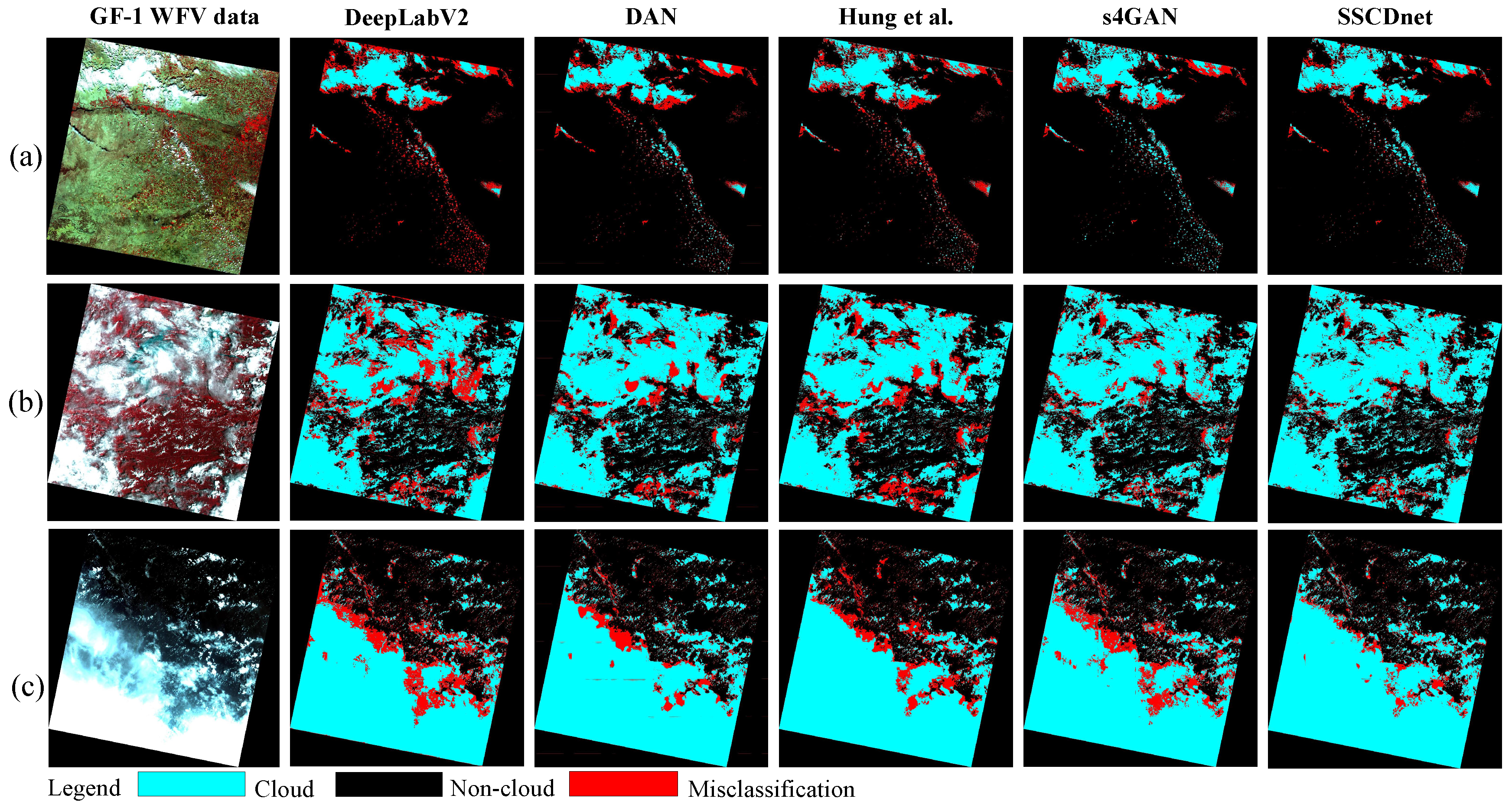
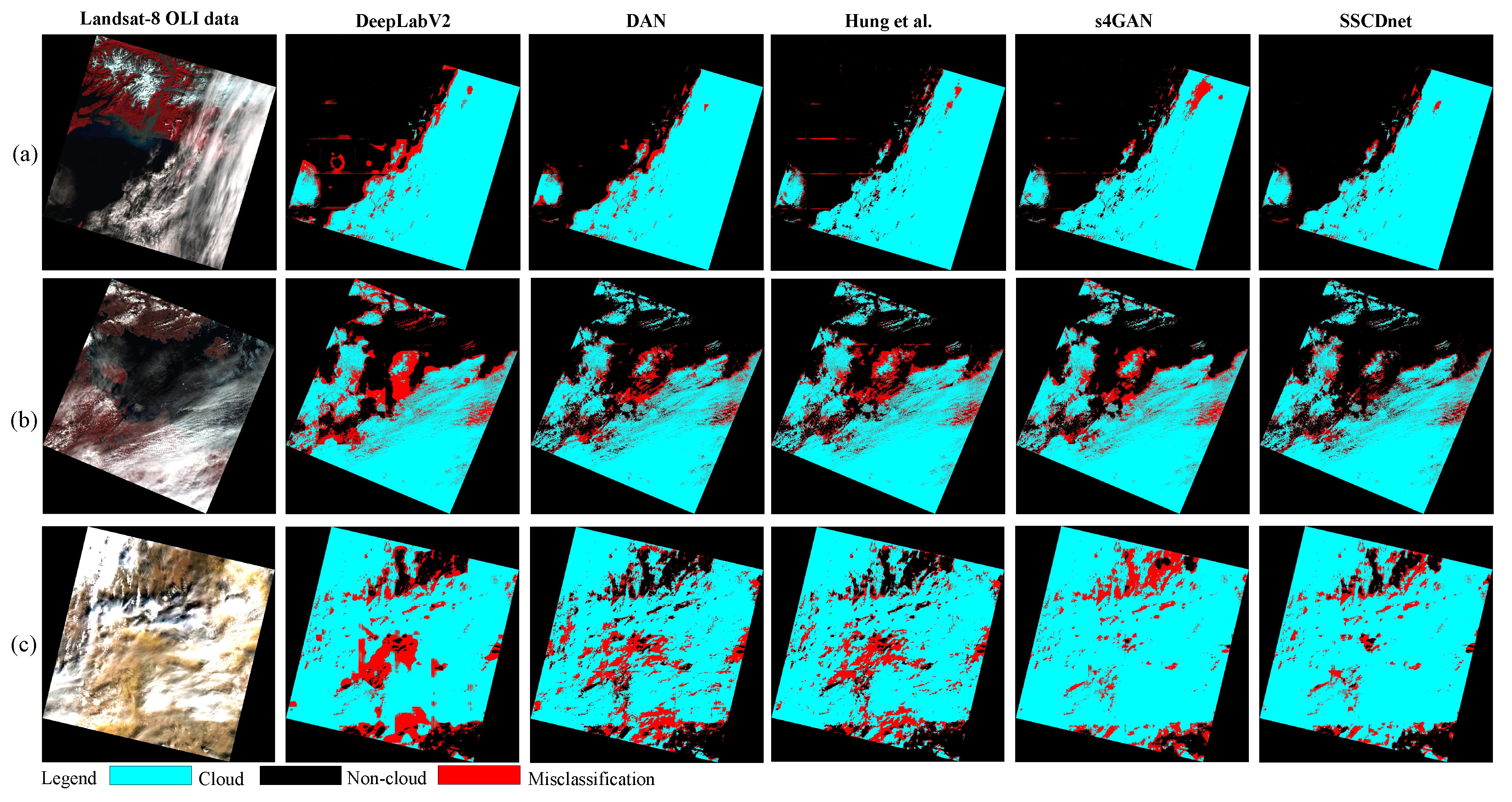
Semi-supervised learning is an effective training strategy, which is able to train a segmentation network by using a limited number of pixel-wise labeled samples and a large number of unlabeled ones. In this paper, we present a semi-supervised cloud detection network, named SSCDnet. Since there are domain distribution gaps between the labeled and unlabeled datasets, we take the domain shift problem into account for the semi-supervised learning framework and propose feature-/output-level domain adaptation strategy to reduce domain distribution gaps, thus improving SSCDnet to generate trustworthy pseudo label for unlabeled data. A high certain pseudo label provides positive supervised signals for segmentation network learning through self-training. Experimental results on GF-1 WFV and Landsat-8 OLI datasets demonstrate that SSCDnet is able to achieve promising performance by using a limited number of labeled samples. It shows great promise for practical application on new satellite RS imagery in the presence of less labeled data available.

Although SSCDnet shows good performance, there is still much room for improvement, such as hyper-parameters setting of loss function and threshold setting of pseudo-labeling. Different cloud detection datasets have different domain distributions. We need to update these parameters to achieve a promising performance on different datasets. In addition, different ground objects have different characteristics, and the performance of SSCDnet on other objects detection also needs to be further evaluated. In our future work, we will further evaluate this method on other cloud detection datasets and other object detection tasks. In addition, SSCDnet performs poorly on cloud boundaries and thin cloud regions, which requires our future efforts to improve it. In our future work, we will also explore how to utilize some auxiliary information, such as land use and land cover (LULC) map, water index map, and vegetation index map, to improve the cloud detection performance.

In general, a semi-supervised learning training strategy provides us with an effective way for cloud detection from RS images in the presence of less labeled data available. In addition, this strategy may provide us a promising way for other object detection tasks such as water, vegetation, and building detection.

In order to promote understanding of the paper’s technology, we released the code of SSCDnet. It is available at: https://github.com/nkszjx/SSCDnet (accessed on 24 April 2022).

References

1. Zhao, S.; Wang, Q.; Li, Y.; Liu, S.; Wang, Z.; Zhu, L.; Wang, Z. An overview of satellite remote sensing technology used in China’s environmental protection. Earth Sci. Inform. 2017, 10, 137–148. [Google Scholar] [CrossRef]
2. Yang, J.; Gong, P.; Fu, R.; Zhang, M.; Chen, J.; Liang, S.; Xu, B.; Shi, J.; Dickinson, R. The role of satellite remote sensing in climate change studies. Nat. Clim. Chang. 2013, 3, 875–883. [Google Scholar] [CrossRef]
3. Schmugge, T.J.; Kustas, W.P.; Ritchie, J.C.; Jackson, T.J.; Rango, A. Remote sensing in hydrology. Adv. Water Resour. 2002, 25, 1367–1385. [Google Scholar] [CrossRef]
4. Shanmugapriya, P.; Rathika, S.; Ramesh, T.; Janaki, P. Applications of remote sensing in agriculture—A Review. Int. J. Curr. Microbiol. Appl. Sci. 2019, 8, 2270–2283. [Google Scholar] [CrossRef]
5. Kabisch, N.; Selsam, P.; Kirsten, T.; Lausch, A.; Bumberger, J. A multi-sensor and multi-temporal remote sensing approach to detect land cover change dynamics in heterogeneous urban landscapes. Ecol. Indic. 2019, 99, 273–282. [Google Scholar] [CrossRef]
6. Bachagha, N.; Wang, X.; Luo, L.; Li, L.; Khatteli, H.; Lasaponara, R. Remote sensing and GIS techniques for reconstructing the military fort system on the Roman boundary (Tunisian section) and identifying archaeological sites. Remote Sens. Environ. 2020, 236, 111418. [Google Scholar] [CrossRef]
7. Guo, J.; Yang, J.; Yue, H.; Tan, H.; Hou, C.; Li, K. CDnetV2: CNN-Based Cloud Detection for Remote Sensing Imagery with Cloud-Snow Coexistence. IEEE Trans. Geosci. Remote Sens. 2020, 59, 700–713. [Google Scholar] [CrossRef]
8. Sliwa, B.; Falkenberg, R.; Liebig, T.; Piatkowski, N.; Wietfeld, C. Boosting vehicle-to-cloud communication by machine learning-enabled context prediction. IEEE Trans. Intell. Transp. Syst. 2019, 21, 3497–3512. [Google Scholar] [CrossRef] [Green Version]
9. Zhu, Z.; Wang, S.; Woodcock, C.E. Improvement and expansion of the Fmask algorithm: Cloud, cloud shadow, and snow detection for Landsats 4–7, 8, and Sentinel 2 images. Remote Sens. Environ. 2015, 159, 269–277. [Google Scholar] [CrossRef]
10. Qiu, S.; He, B.; Zhu, Z.; Liao, Z.; Quan, X. Improving Fmask cloud and cloud shadow detection in mountainous area for Landsats-8 images. Remote Sens. Environ. 2017, 199, 107–119. [Google Scholar] [CrossRef]
11. Qiu, S.; Zhu, Z.; He, B. Fmask 4.0: Improved cloud and cloud shadow detection in Landsats 4–8 and Sentinel-2 imagery. Remote Sens. Environ. 2019, 231, 111205. [Google Scholar] [CrossRef]
12. Li, Z.; Shen, H.; Li, H.; Xia, G.; Gamba, P.; Zhang, L. Multi-feature combined cloud and cloud shadow detection in GaoFen-1 wide field of view imagery. Remote Sens. Environ. 2017, 191, 342–358. [Google Scholar] [CrossRef] [Green Version]
13. Alonso-Montesinos, J.; Martínez-Durbán, M.; del Sagrado, J.; del Águila, I.; Batlles, F. The application of Bayesian network classifiers to cloud classification in satellite images. Renew. Energy 2016, 97, 155–161. [Google Scholar] [CrossRef]
14. Xu, L.; Wong, A.; Clausi, D.A. A novel Bayesian spatial–temporal random field model applied to cloud detection from remotely sensed imagery. IEEE Trans. Geosci. Remote Sens. 2017, 55, 4913–4924. [Google Scholar] [CrossRef]
15. Latry, C.; Panem, C.; Dejean, P. Cloud detection with SVM technique. In Proceedings of the 2007 IEEE International Geoscience and Remote Sensing Symposium, Barcelona, Spain, 23–27 July 2007; pp. 448–451. [Google Scholar]
16. Ishida, H.; Oishi, Y.; Morita, K.; Moriwaki, K.; Nakajima, T.Y. Development of a support vector machine based cloud detection method for MODIS with the adjustability to various conditions. Remote Sens. Environ. 2018, 205, 390–407. [Google Scholar] [CrossRef]
17. Hughes, M.J.; Hayes, D.J. Automated detection of cloud and cloud shadow in single-date Landsat imagery using neural networks and spatial post-processing. Remote Sens. 2014, 6, 4907–4926. [Google Scholar] [CrossRef] [Green Version]
18. Jang, J.d.; Viau, A.A.; Anctil, F.; Bartholomé, E. Neural network application for cloud detection in SPOT VEGETATION images. Int. J. Remote Sens. 2006, 27, 719–736. [Google Scholar] [CrossRef]
19. Jeppesen, J.H.; Jacobsen, R.H.; Inceoglu, F.; Toftegaard, T.S. A cloud detection algorithm for satellite imagery based on deep learning. Remote Sens. Environ. 2019, 229, 247–259. [Google Scholar] [CrossRef]
20. Wieland, M.; Li, Y.; Martinis, S. Multi-sensor cloud and cloud shadow segmentation with a convolutional neural network. Remote Sens. Environ. 2019, 230, 111203. [Google Scholar] [CrossRef]
21. Chai, D.; Newsam, S.; Zhang, H.K.; Qiu, Y.; Huang, J. Cloud and cloud shadow detection in Landsat imagery based on deep convolutional neural networks. Remote Sens. Environ. 2019, 225, 307–316. [Google Scholar] [CrossRef]
22. Drönner, J.; Korfhage, N.; Egli, S.; Mühling, M.; Thies, B.; Bendix, J.; Freisleben, B.; Seeger, B. Fast cloud segmentation using convolutional neural networks. Remote Sens. 2018, 10, 1782. [Google Scholar] [CrossRef] [Green Version]
23. Lopez, J.; Santos, S.; Atzberger, C.; Torres, D. Convolutional Neural Networks for Semantic Segmentation of Multispectral Remote Sensing Images. In Proceedings of the 2018 IEEE 10th Latin-American Conference on Communications (LATINCOM), Guadalajara, Mexico, 14–16 November 2018; pp. 1–5. [Google Scholar]
24. Zhan, Y.; Wang, J.; Shi, J.; Cheng, G.; Yao, L.; Sun, W. Distinguishing cloud and snow in satellite images via deep convolutional network. IEEE Geosci. Remote Sens. Lett. 2017, 14, 1785–1789. [Google Scholar] [CrossRef]
25. Morales, G.; Huamán, S.G.; Telles, J. Cloud Detection in High-Resolution Multispectral Satellite Imagery Using Deep Learning. In Proceedings of the International Conference on Artificial Neural Networks, Rhodes, Greece, 4–7 October 2018; pp. 280–288. [Google Scholar]
26. Li, Z.; Shen, H.; Cheng, Q.; Liu, Y.; You, S.; He, Z. Deep learning based cloud detection for medium and high resolution remote sensing images of different sensors. ISPRS J. Photogramm. Remote Sens. 2019, 150, 197–212. [Google Scholar] [CrossRef] [Green Version]
27. Yang, J.; Guo, J.; Yue, H.; Liu, Z.; Hu, H.; Li, K. CDnet: CNN-Based Cloud Detection for Remote Sensing Imagery. IEEE Trans. Geosci. Remote Sens. 2019, 57, 6195–6211. [Google Scholar] [CrossRef]
28. Shao, Z.; Pan, Y.; Diao, C.; Cai, J. Cloud Detection in Remote Sensing Images Based on Multiscale Features-Convolutional Neural Network. IEEE Trans. Geosci. Remote Sens. 2019, 57, 4062–4076. [Google Scholar] [CrossRef]
29. Chen, Y.; Weng, Q.; Tang, L.; Liu, Q.; Fan, R. An Automatic Cloud Detection Neural Network for High-Resolution Remote Sensing Imagery With Cloud–Snow Coexistence. IEEE Geosci. Remote Sens. Lett. 2022, 19, 6004205. [Google Scholar] [CrossRef]
30. Zhang, Z.; Iwasaki, A.; Xu, G.; Song, J. Cloud detection on small satellites based on lightweight U-net and image compression. J. Appl. Remote Sens. 2019, 13, 026502. [Google Scholar] [CrossRef]
31. Zhang, J.; Li, X.; Li, L.; Sun, P.; Su, X.; Hu, T.; Chen, F. Lightweight U-Net for cloud detection of visible and thermal infrared remote sensing images. Opt. Quantum Electron. 2020, 52, 397. [Google Scholar] [CrossRef]
32. Li, J.; Wu, Z.; Hu, Z.; Jian, C.; Luo, S.; Mou, L.; Zhu, X.X.; Molinier, M. A Lightweight Deep Learning-Based Cloud Detection Method for Sentinel-2A Imagery Fusing Multiscale Spectral and Spatial Features. IEEE Trans. Geosci. Remote Sens. 2021, 60, 1–19. [Google Scholar] [CrossRef]
33. Guo, J.; Yang, J.; Yue, H.; Li, K. Unsupervised Domain Adaptation for Cloud Detection Based on Grouped Features Alignment and Entropy Minimization. IEEE Trans. Geosci. Remote Sens. 2021, 1–13. [Google Scholar] [CrossRef]
34. Guo, J.; Yang, J.; Yue, H.; Liu, X.; Li, K. Unsupervised Domain-Invariant Feature Learning for Cloud Detection of Remote Sensing Images. IEEE Trans. Geosci. Remote Sens. 2022, 60, 5405715. [Google Scholar] [CrossRef]
35. Guo, J.; Yang, J.; Yue, H.; Chen, Y.; Hou, C.; Li, K. Cloud Detection From Remote Sensing Imagery Based on Domain Translation Network. IEEE Geosci. Remote Sens. Lett. 2022, 19, 5000805. [Google Scholar] [CrossRef]
36. Cordts, M.; Omran, M.; Ramos, S.; Rehfeld, T. The Cityscapes Dataset for Semantic Urban Scene Understanding. arXiv 2016, arXiv:1604.01685. [Google Scholar]
37. Zhang, Y.; Yang, L.; Chen, J.; Fredericksen, M.; Hughes, D.P.; Chen, D.Z. Deep Adversarial Networks for Biomedical Image Segmentation Utilizing Unannotated Images. In Proceedings of the Medical Image Computing and Computer Assisted Intervention (MICCAI 2017), Quebec City, QC, Canada, 11–13 September 2017; pp. 408–416. [Google Scholar]
38. Hong, S.; Noh, H.; Han, B. Decoupled Deep Neural Network for Semi-supervised Semantic Segmentation. arXiv 2015, arXiv:1506.04924. [Google Scholar]
39. Mostafa S, I.; Arash, V.; Mani, R.; William G, M. Semi-Supervised Semantic Image Segmentation with Self-correcting Networks. arXiv 2020, arXiv:1811.07073. [Google Scholar]
40. Mittal, S.; Maxim, T.; Thomas, B. Semi-Supervised Semantic Segmentation with High- and Low-level Consistency. IEEE Trans. Pattern Anal. Mach. Intell. 2021, 43, 1369–1379. [Google Scholar] [CrossRef] [Green Version]
41. Massih-Reza, A.; Vasilii, F.; Loic, P.; Emilie, D.; Yury, M. Self-Training: A Survey. arXiv 2022, arXiv:2202.12040. [Google Scholar]
42. Rajat, R.; Alexis, B.; Honglak, L.; Benjamin, P.; Andrew, Y.N. Self-taught learning: Transfer learning from unlabeled data. In Proceedings of the Twenty-fourth International Conference on Machine Learning, Corvalis, OR, USA, 20–24 June 2007. [Google Scholar]
43. Hung, W.; Tsai, Y.; Liou, Y.; Lin, Y.Y.; Yang, M.H. Adversarial Learning for Semi-Supervised Semantic Segmentation. arXiv 2018, arXiv:1802.07934. [Google Scholar]
44. Goodfellow, I.; Pouget-Abadie, J.; Mirza, M.; Xu, B.; Warde-Farley, D.; Ozair, S.; Courville, A.; Bengio, Y. Generative adversarial networks. In Proceedings of the Advances in Neural Information Processing Systems, Montreal, QC, Canada, 8–13 December 2014; pp. 2672–2680. [Google Scholar]
45. Ren, Z.; Lee, Y.J. Cross-Domain Self-Supervised Multi-task Feature Learning Using Synthetic Imagery. In Proceedings of the 2018 IEEE/CVF Conference on Computer Vision and Pattern Recognition, Salt Lake City, UT, USA, 18–22 June 2018; pp. 762–771. [Google Scholar]
46. Tuan-Hung, V.; Himalaya, J.; Maxime, B.; Matthieu, C.; Patrick, P. ADVENT: Adversarial Entropy Minimization for Domain Adaptation in Semantic Segmentation. arXiv 2019, arXiv:1811.12833. [Google Scholar]
47. Tsai, Y.; Sohn, K.; Schulter, S.; Chandraker, M. Domain Adaptation for Structured Output via Discriminative Patch Representations. In Proceedings of the 2019 IEEE/CVF International Conference on Computer Vision, Seoul, Korea, 27 October–2 November 2019; pp. 1456–1465. [Google Scholar]
48. Foga, S.; Scaramuzza, P.L.; Guo, S.; Zhu, Z.; Dilley, R.D., Jr.; Beckmann, T.; Schmidt, G.L.; Dwyer, J.L.; Hughes, M.J.; Laue, B. Cloud detection algorithm comparison and validation for operational Landsat data products. Remote Sens. Environ. 2017, 194, 379–390. [Google Scholar] [CrossRef] [Green Version]
49. Chen, Y.; Lin, Y.; Yang, M.; Huang, J. CrDoCo: Pixel-Level Domain Transfer With Cross-Domain Consistency. In Proceedings of the 2019 IEEE/CVF Conference on Computer Vision and Pattern Recognition, Long Beach, CA, USA, 16–20 June 2019; pp. 1791–1800. [Google Scholar]
50. Souly, N.; Spampinato, C.; Shah, M. Semi Supervised Semantic Segmentation Using Generative Adversarial Network. In Proceedings of the 2017 IEEE International Conference on Computer Vision (ICCV), Venice, Italy, 22–29 October 2017; pp. 5689–5697. [Google Scholar]
51. Chen, L.; Papandreou, G.; Kokkinos, I.; Murphy, K.; Yuille, A.L. DeepLab: Semantic Image Segmentation with Deep Convolutional Nets, Atrous Convolution, and Fully Connected CRFs. IEEE Trans. Pattern Anal. Mach. Intell. 2018, 40, 834–848. [Google Scholar] [CrossRef] [PubMed] [Green Version]
52. He, K.; Zhang, X.; Ren, S.; Sun, J. Deep Residual Learning for Image Recognition. In Proceedings of the The IEEE Conference on Computer Vision and Pattern Recognition (CVPR), Las Vegas, NV, USA, 27–30 June 2016. [Google Scholar]
53. Yu, F.; Koltun, V. Multi-Scale Context Aggregation by Dilated Convolutions. arXiv 2016, arXiv:1511.07122. [Google Scholar]
54. Geirhos, R.; Rubisch, P.; Michaelis, C.; Bethge, M.; Wichmann, F.A.; Brendel, W. ImageNet-trained CNNs are biased towards texture; increasing shape bias improves accuracy and robustness. arXiv 2018, arXiv:1811.12231. [Google Scholar]
55. Bengio, Y. Practical recommendations for gradient-based training of deep architectures. In Neural Networks: Tricks of the Trade; Springer: Berlin/Heidelberg, Germany, 2012; pp. 437–478. [Google Scholar]
56. Kingma, D.; Ba, J. Adam: A Method for Stochastic Optimization. arXiv 2014, arXiv:1412.6980v9. [Google Scholar]
57. Chen, L.C.; Papandreou, G.; Schroff, F.; Adam, H. Rethinking atrous convolution for semantic image segmentation. arXiv 2017, arXiv:1706.05587. [Google Scholar]
58. Russakovsky, O.; Deng, J.; Su, H.; Krause, J.; Satheesh, S.; Ma, S.; Huang, Z.; Karpathy, A.; Khosla, A.; Bernstein, M.; et al. Imagenet large scale visual recognition challenge. Int. J. Comput. Vis. 2015, 115, 211–252. [Google Scholar] [CrossRef] [Green Version]
59. Everingham, M.; Van Gool, L.; Williams, C.K.I.; Winn, J.; Zisserman, A. The PASCAL Visual Object Classes Challenge 2012 (VOC2012) Results. Available online: http://host.robots.ox.ac.uk/pascal/VOC/voc2012/ (accessed on 24 April 2022).
Figure 1. The traditional semi-supervised segmentation framework.
Remotesensing 14 02641 g001
Figure 2. Remote sensing images obtained from the same satellite sensor (GF-1 satellite) at different places. Where (a) GF1_WFV2_E127.2_N45.9_20140704_L2A00003099760, (b) GF1_WFV1_E102.0_N28.0_20140302_L2A00002804760, (c) GF1_WFV1_E99.4_N36.3_20140716_L2A00002789230, and (d) GF1_WFV3_E89.3_N35.6_20140702_L2A00008451540.
Remotesensing 14 02641 g002
Figure 3. The detailed structure of the proposed SSCDnet.
Remotesensing 14 02641 g003
Figure 4. Structure of the proposed class-relevant feature alignment module.
Remotesensing 14 02641 g004
Figure 5. Structure of the proposed CROA.
Remotesensing 14 02641 g005
Figure 6. Experiment results on an unlabeled remote sensing image. (a) input GF-1 WFV image; (b) un-applied domain adaptation result, and (c) applied domain adaptation result.
Remotesensing 14 02641 g006
Figure 7. The double threshold pseudo-labelling method for self-training.
Remotesensing 14 02641 g007
Figure 8. Structure of the proposed discriminator network.
Remotesensing 14 02641 g008
Figure 9. Comparison of cloud detection results of different methods on GF-1 WFV dataset with labeled sample proportion of 1/200. Image ID of (a), (b), and (c) are GF1_WFV2_W102.1_N37.6_20140517_L2A0000244678, GF1_WFV3_E114.1_N2.1_20151011_L2A0001094727, and GF1_WFV3_E87.8_N2.1_20140316_L2A0000184430, respectively.
Remotesensing 14 02641 g009
Figure 10. Comparison of cloud extraction results of different methods on Landsat-8 OLI dataset with a labeled sample proportion of 1/200. The image ID of (a), (b), and (c) are LC80650182013237LGN00, LC80430122014214LGN00, and LC81990402014267LGN00, respectively.
Remotesensing 14 02641 g010
Figure 11. Cloud extraction results of SSCDnet on Landsat-8 OLI data under different seasons (labeled proportion is 1 20 ). Where, (a) is the Spring season (ID: LC08_L1TP_122033_20160411_20170326_01_T1), (b) is the Summer season (ID: LC08_L1TP_122033_20180706_20180717_01_T1), (c) is the Autumn season(ID: LC08_L1TP_122033_20181111_20181127_01_T1), and (d) is the Winter season (ID: LC08_L1TP_122033_20150103_20170415_01_T1).
Remotesensing 14 02641 g011
Figure 12. Cloud extraction results (1200 × 1200) of SSCDnet on Landsat-8 OLI data under different land cover types. Where, (a,b) are barren/desert areas. (c,d) are mountain/plant areas. (e,f) are farmland/villages areas. (g,h) are urban/river areas. (i,j) are mountain/lake areas. (k,l) are ocean areas.
Remotesensing 14 02641 g012
Figure 13. Cloud extraction results (1200 × 1200) of SSCDnet on GF-1 WFV and Landsat-8 OLI data under different labeled sample proportions. (a,b) are the results of GF-1 WFV data (GF1_WFV2_W70.8_N19.2_20140801_L2A0000292230), while (c,d) are the results of Landsat-8 OLI data (LC81180382014244LGN00).
Remotesensing 14 02641 g013